metrology and numerical characterization of random rough

Original Article

Metrology and numerical characterizationof random rough surfaces—Datareduction via an effective filtering solution

Itzhak Green

Abstract

Random rough surfaces appear in measurements as noisy signals varying spatially. Mathematically, there is no theoretical

difference between such and time-varying signals. Hence, the extensive array of methods and analysis tools that have

been developed for signal processing are available also for rough surfaces characterization. In both, the objective is to

reduce the vast amount of data to just a few meaningful parameters that allow the application of other physical concepts.

Particularly in contact mechanics, it is well known that the Greenwood–Williamson model requires three parameters for

the calculation of the elastic deformation of rough surface asperities. The parameters are the roughness standard

deviation, the equivalent asperity radius, and the asperity density. These parameters are byproducts of the spectral

moments. The spectral moments have been employed for decades in many fields of engineering and science. For rough

surfaces, for example, the work by McCool outlines a mathematical blueprint procedure on how to straightforwardly

reduce the entire roughness data into the said three spectral moments. It is commonly claimed, however, that the said

procedure inherently suffers from resolution problems, that is, a given surface shall have much different spectral

moments depending on the sampling rate (or spacing). To study these issues, synthetic surfaces are generated herein

using a harmonic waveform precisely as McCool had done. However, here the signals are contaminated by a white noise

process with various magnitudes. A signal-to-noise ratio is defined and used to assess the quality of the signal, and the

spectral moments are evaluated for various magnitudes of the noise. Since closed-from solutions are available for the

spectral moments of the uncontaminated signal, the contaminated signals are evaluated vis-a-vis the exact anticipated

values, and the errors are calculated. It is shown that using the common techniques (such as those outlined by McCool)

can lead to enormous and unacceptable errors. Resolution is studied as well; it is shown to have an effect only in the

presence of noise, but by itself it has no independent influence on the spectral moments. The venerable Savitzky–Golay

smoothing filter is used on the noisy signals, showing some improvements, but the resulting spectral moments predicted

still contain objectionable errors. A generalized exponential smoothing filter, G-EXP, is constructed, and it is shown to

markedly moderate the errors and reduce them to acceptable levels, while effectively restoring the underlying surface

physical characteristics. Moreover, the filtered signals do not suffer from resolution problems, where results, in fact,

improve with higher (i.e., finer) resolutions. Fractal-generated signals are likewise discussed.

Keywords

Surface roughness, surface metrology, spectral moments, white noise contamination, signal processing, signal-to-noise

ratio, filter design, Savitzky–Golay filtering

Date received: 15 May 2019; accepted: 7 October 2019

Introduction

This work puts emphasis on data reduction regardingrough surfaces for the purpose of contact mechanicscalculation, but the concepts herein apply equally wellto the processing of any signal contaminated by arandom noise.

The Greenwood–Williamson (GW)1 approach tomodeling the contact of two elastic rough surfaces hasgained wide acceptance. The approach reduces the tworough surfaces into a single equivalent rough surface that

is forced against a perfectly smooth and rigid flat. Thecommon assumptions are that the equivalent surface hasasperities that deform independently of the neighboring

GWW School of Mechanical Engineering, Georgia Institute of

Technology, Atlanta, GA, USA

Corresponding author:

Itzhak Green, GWW School of Mechanical Engineering, Georgia

Institute of Technology, Atlanta, GA, USA.

Email: [email protected]

Proc IMechE Part J:

J Engineering Tribology

0(0) 1–18

! IMechE 2019

Article reuse guidelines:

sagepub.com/journals-permissions

DOI: 10.1177/1350650119885281

journals.sagepub.com/home/pij

https://uk.sagepub.com/en-gb/journals-permissions

https://doi.org/10.1177/1350650119885281

journals.sagepub.com/home/pij

http://crossmark.crossref.org/dialog/?doi=10.1177%2F1350650119885281&domain=pdf&date_stamp=2019-11-22

asperities, all asperities have an equivalent radius,R, theyhave an areal density, Z, and that they are distributed bysome probability density function. At the time of itsdevelopment (1966), in the absence of a closed-formsolution for a Gaussian distribution, GW used an expo-nential distribution that could be solved analytically inclosed-form, which led to some physical conclusions.However, even GW state and show that surfaces’height distribution tends to be Gaussian rather thanexponential. It was not until 2011 that Jackson andGreen2 provided a closed-form solution to the GWmodel using an uncompromised Gaussian distribution.That work2 has also demonstrated the resolution issuewhere the same measured data of real rough surfaces canprovide very different spectral moments depending onthe spacing (see Table 1 there).

The GW has gained acceptance in contact of roughsurfaces even under elasto-plastic loading.3–5 Lackingin the original GW work, however, is the mathematicalprocess of reducing the two rough surface propertiesinto a single rough one. The work by McCool6 fills thisgap by providing a complete mathematical blueprinton how two surfaces having three-dimensional (3D),orthotropic roughness, z¼ z(x,y), can be convertedinto the desired single surface having a compositeroughness. That work6 allows, without loss of general-ity, to employ two-dimensional (2D) roughness quan-tities, and that is precisely what is considered herein,i.e. z¼ z(x). As also summarized by McCool,6,7 thethree quantities m0, m2, and m4, known as the spectralmoment, are sufficient to completely define all the par-ameters needed in the GW model. These moments canbe obtained in the spatial domain by

m0 ¼1

N

XNi¼1

zð Þ2i ð1Þ

m2 ¼1

N

XNi¼1

dz

dx

� �2

i

ð2Þ

m4 ¼1

N

XNi¼1

d 2z

dx2

� �2

i

ð3Þ

where N is the total number of data points sampled ona surface along a generic coordinate x, while z¼ z(x)is the asperity height measured from the mean surface.In the said works,6,7 an alternative method is pro-pounded by using the power spectrum P(!) of thewaveform z(x) to yield the kth moments

mk ¼

Z 10

!kP !ð Þd! @ k ¼ 0, 2, 4 ð4Þ

Here, ! ¼ 2� f ¼ 2�=l, where ! is the circular fre-quency of f and l is the wavelength (being equivalentto the period had z¼ z(t) been a waveform in time, t).Note that for k¼ 0, equation (4) signifies Parseval’stheorem. For additional information, see Sweitzeret al.;8 Davidson and Loughlin;9 Vogel;10 andBrown.11 Evidently, these moments are not specificto modeling surface roughness just in tribology, asthey are central in the many fields of science andengineering, falling generally into the category ofsignal processing for which there is ample literature,see notably the excellent classical texts by Bendat andPiersol.12–14 Non-tribological examples can rangefrom geomechanics of rough wall fracture11 tosignal processing performed on the output from thepulsed laser photoacoustic instrument monitoringcrude oil in water,10 or in the analysis an optical tele-scope.8 Specifically, in tribology though, these three

Table 1. Values of the exact spectral moments and their numerically calculated values with relative errors for various noise

amplitudes, �A, and resolutions, dx.

At �A ¼ 0

m0¼ 1/2¼ 0.5 m2 ¼ 2�2 ¼ 19:739 m4 ¼ 8�4 ¼ 779:27

�¼ 1 SNRdB ¼ 1Value Error % Value Error % Value Error %

nfft¼ 9, �x ¼ 0:012272

�A ¼ 1% 0.503 0.5 19.87 0.7 16681.1 2.04E3 21.24 41.5

�A ¼ 10% 0.508 1.7 42.04 113 1.591E6 2.04E5 457.8 21.5

�A ¼ 30% 0.541 8.3 220.7 1018 1.432E7 1.84E6 159.3 12.2

nfft¼ 11, �x ¼ 0:003068

�A ¼ 1% 0.503 0.5 22.9 16.23 3.830E6 4.91E5 3656.7 41.5

�A ¼ 10% 0.505 1.1 349.3 1669 3.829E8 4.91E7 1586.0 21.5

�A ¼ 30% 0.531 6.2 2986 1.5E4 3.446E9 4.42E8 205.22 12.2

nfft¼ 12, �x ¼ 0:001534

�A ¼ 1% 0.503 0.5 32.5 64.52 5.846E7 7.50E6 27865 41.5

�A ¼ 10% 0.506 1.3 1303.9 6505 5.846E9 7.50E8 1741.5 21.5

�A ¼ 30% 0.534 6.8 11578 5.9E4 5.26E10 6.75E9 209.61 12.2

Notes: Given also are the bandwidth parameter, �, and the signal-to-noise ratio in (dB). For all cases, A¼ 1 m and f¼ 1 Hz.

2 Proc IMechE Part J: J Engineering Tribology 0(0)

moments are sufficient to execute the GW model, andthey are focal in this work.

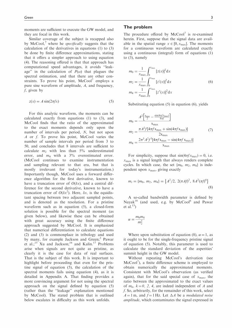
Similar coverage of the subject is recapped alsoby McCool,7 where he specifically suggests that thecalculation of the derivatives in equations (1) to (3)be done by finite difference approximations, statingthat it offers a simpler approach to using equation(4). The reasoning offered is that that approach hascomputational speed advantages, it avoids ‘‘leak-age’’ in the calculation of P(!) that plagues thespectral estimation, and that there are other con-straints. To prove his point, McCool7 employs apure sine waveform of amplitude, A, and frequency,f, given by

z xð Þ ¼ A sin 2�fxð Þ ð5Þ

For this analytic waveform, the moments can becalculated exactly from equations (1) to (3), andMcCool finds that the ratio of the approximatedto the exact moments depends only upon thenumber of intervals per period, N, but not uponA or f. To prove his point, McCool varies thenumber of sample intervals per period from 3 to50, and concludes that 8 intervals are sufficient tocalculate m2 with less than 5% underestimatederror, and m4 with a 3% overestimated error.(McCool continues to examine instrumentationand sampling relevant to that era, but that ismostly irrelevant for today’s instrumentation.)Importantly though, McCool uses a forward differ-ence algorithm for the first derivative, known tohave a truncation error of O(�x), and a central dif-ference for the second derivative, known to have atruncation error of O(�x2). Here, �x, is the equidis-tant spacing between two adjacent sampled points,and is denoted as the resolution. For a pristinewaveform such as in equation (5), a closed-formsolution is possible for the spectral moment (asgiven below), and likewise these can be obtainedwith great accuracy using the finite differenceapproach suggested by McCool. It is emphasizedthat numerical differentiation to calculate equations(2) and (3) is commonplace in tribology and usedby many, for example Jackson and Green;2 Pawaret al.;15 Xu and Jackson;16 and Kalin.17 Problemsarise when signals are not quite as pristine, asclearly it is the case for data of real surfaces.That is the subject of this work. It is important tohighlight before proceeding that even for the pris-tine signal of equation (5), the calculation of thespectral moments fails using equation (4), as it isdetailed in Appendix A. That finding provides amore convincing argument for not using the spectralapproach on the signal defined by equation (5)(rather than the ‘‘leakage’’ explanation mentionedby McCool). The stated problem that is outlinedbelow escalates in difficulty as this work unfolds.

The problem

The procedure offered by McCool7 is re-examinedherein. First, suppose that the signal data are avail-able in the spatial range x 2 0, xmax½ �. The momentsfor a continuous waveform are calculated exactlyusing a continuous (integral) form of equations (1)to (3), namely

m0 ¼1

xmax

Z xmax

0

z xð Þ½ �2dx

m2 ¼1

xmax

Z xmax

0

z0 xð Þ½ �2dx

m4 ¼1

xmax

Z xmax

0

z00 xð Þ½ �2dx

ð6Þ

Substituting equation (5) in equation (6), yields

m0 ¼A2 xmax

2 �sin 4�f xmaxð Þ

8�f

h ixmax

m2 ¼�A2f ½4�f xmax þ sin 4�f xmaxð Þ�

2xmax

m4 ¼2�3A2f 3 4�f xmax � sin 4�f xmaxð Þ½ �

xmax

ð7Þ

For simplicity, suppose that sin 4�fxmaxð Þ ¼ 0, i.e.xmax is a signal length that always renders completecycles. In which case, the set m0, m2, m4f g is inde-pendent upon xmax, giving exactly

mt ¼ m0, m2, m4f g ¼ A2=2, 2 �Afð Þ2, 8A2 �fð Þ4

� �ð8Þ

A so-called bandwidth parameter is defined byNayak18 (and used, e.g. by McCool6 and Pawaret al.15)

� ¼m0m4

m22

Where upon substitution of equation (8), �¼ 1, asit ought to be for the single-frequency pristine signalof equation (5). Notably, this parameter is used tocalculate the standard deviation of the asperities’summit height in the GW model.

Without repeating McCool’s derivation (seeMcCool7), a finite difference scheme is employed toobtain numerically the approximated moments.Consistent with McCool’s observation (as verifiedagain), that for the said special case of xmax, theratio between the approximated to the exact valuesof mk, k¼ 0, 2, 4, are indeed independent of A andf. So, arbitrarily, for the remainder of this work, selectA¼ 1m, and f¼ 1Hz. Let �A be a modulated noiseamplitude, which contaminates the signal expressed in

Green 3

equation (5). Hence, when �A¼ 0, there is no noise,and the first row in Table 1 represents the results ofthe ‘‘pristine’’ or ‘‘ideal’’ signal. For that case, themoments are provided exactly, as well as by theirnumerical values. The noise amplitude �A shall beelaborated upon shortly, as it greatly affects thenumerical values of the spectral moments, which arethe objectives (i.e. target values) of this work. Alsogiven are the bandwidth parameter as discussedabove and the signal-to-noise ratio (SNR) (which isdefined and discussed below).

So, the signal in equation (5) is an ideal (i.e. ‘‘pris-tine’’) sine wave, and that is the signal that McCool7

focused upon. However, that is an unrealistic expect-ation for the behavior of real surfaces. Clearly, realsurfaces shall always exhibit some noise in the mea-sured signal (where in fact quite frequently, consid-erable noise should be expected10,19,20). Suppose thata random noise process of magnitude �A issuperimposed upon the pure sine waveform of equa-tion (5). The entire signal is constructed using thefollowing Mathematica script (again for A¼ 1mand f¼ 1Hz)

w ¼ 2�; nfft ¼ 9;

n ¼ 2 ^ nfftþ 1; delx ¼ 2�= n� 1ð Þ;

x ¼ Table i� 1ð Þ � delx, i, 1, nf g½ �;

signal ¼ Sin½w � x�;

SeedRandom 1234½ �; �A ¼ 0 � 0:01;

noise ¼ �A � Table RandomReal �1, 1f g½ �, i, 1, nf g½ �;

z ¼ signalþ noise

ð9Þ

The variable z¼ z(x) in equation (9) is evidentlycomposed of a pure sine waveform signal of equation(5) having an assigned circular frequency, w, and awhite noise contamination having a uniform distribu-tion in the range {–1, 1}, where the noise is modulatedby an amplitude, �A. The arbitrary seed of 1234guarantees that all noise cases analyzed herein shallalways have the same white noise content throughout(By using the Mathematica script given in equation(9), along with the parameters in Table 1, all theresults in this work can be straightforwardly repli-cated.). The lengths of the signals (the pure waveformand the noise) are set to be powers of 2 via the nfftexponent parameter. That is a convenience to helpwith a fast Fourier transform, when taken. Clearly,that parameter also decides the resolution, �x (asdetermined by equation (9), and given in Table 1).

To calculate the derivatives in this work, thefirst and second derivatives are calculated by a finitedifference scheme using a five-point approximation(see Hildebrand,21 p. 111). Corresponding tonfft¼ {9,11,12}, the number of points are n¼ {513,2049, 4097}, and the truncation errors, for both first

and second derivatives, are of order,O(�x4)¼ {2.27*10–8, 8.86*10–11, 5.54*10–12}, respect-ively. This is opposed to McCool’s n¼ 51, having thefinest truncation errors of orders, O(�x)¼ 0.02, forthe first derivative, and O(�x2)¼ 4*10–4, for thesecond derivative. Hence, in the current work, theestimations for the derivatives are of truncationerrors of at least four orders of magnitude smaller(better) than McCool’s calculations. Also, six cyclesare used herein (see Figure 1), where McCool usesonly one cycle. Clearly, the numerical procedureused herein is considerably more accurate androbust than McCool’s procedure.7 To verify the val-idity of the current numerical procedure, the noiseamplitude is set first to zero in equation (9), i.e.�A ¼ 0, and the numerical results obtained forthe moments turn out to be identical to those of theexact predictions (with no error visible within the firstsix (6) significant digits). That is true for any reso-lution, �x. With that, the numerical derivative proced-ure used herein is verified. It is explicitly emphasizedthat in this work, only the five-point finite differencescheme of higher order O(�x4) is used to calculate thenumerical derivatives.

Now, Table 1 summarizes the spectral momentvalues along with the deviation from the exact valuefor other values of �A and nfft, i.e. �x, which arevaried in equation (9). The deviation, or relativeerror, is calculated according to ‘‘100%*abs(exact_va-lue – numerical_value) / exact_value’’. The details areas follows.

To start off, a tiny random noise amplitude of 1%is tacked upon the signal (i.e. �A ¼ 0:01m).Figure 1(a) shows an ideal sine wave signal, equation(5), and its exact first and second derivatives in blackcolor. The noisy signal and its respective numericalderivatives are shown in red color. When the puresine waveform and the noisy signal are plottedtogether (left most plot in Figure 1(a)), it is nearlyimpossible to tell the difference between the two sig-nals. However, the first derivative already shows somedeviation from the exact solution near the inflectionpoints, while the second derivative is hugely over-esti-mated throughout.

The zeroth moment m0 contains no derivativesand, hence, it is predicted nearly exactly for anyresolution, as shown in Table 1. The secondmoment m2 is affected by the errors in the firstderivative, and when averaging takes place by equa-tion (2), the error varies from 0.7% to 16.23%, andthen to 64.52% depending on the resolution.However, the fourth moment m4 is affected signifi-cantly by the huge errors in the second derivative,and when averaging takes place by equation (3), theerror varies from 2040% to 7.5� 106%. That cannotbe considered acceptable under any circumstances.The bandwidth parameter, �, which should haveequaled unity, is also grossly overestimated, rangingfrom 21.24 to 27,865.


If all that happens just for a tiny noise of 1% thatcontaminates the signal, matters can only get worsewith larger noise levels. Practically, there is alwaysnoise in the measuring equipment in addition to thefact that real surfaces are simply imperfect. It is alsointuitively understood that such small noise levelsshould not have a meaningful effect when the surfacesare brought (loaded) into contact, because suchsmall surface undulation would be structurally‘‘weak,’’ and they will be leveled (smashed) by theinitial application of a normal load. However, withsuch large errors in m2 and particularly m4, the neces-sary GW parameters cannot be considered trust-worthy even for a 1% noise level. Moreover, itseems that indeed, the errors exacerbate with therefinement of the resolution, a phenomenon that isanalyzed in detail hereunder.

Next, larger contaminations are investigated.Suppose that the noise magnitude has a moderatelylarger value of 10% (i.e. �A ¼ 0:1m, see Figure 1(b)).The errors in the prediction of the moments m2 andm4 are expected to worsen, and indeed they escalaterather significantly, as indicated in Table 1. And whenthe noise level is 30% (see Figure 1(c)), the predictionsof m2 and m4 are practically useless. Likewise, thebandwidth parameter, a, is very much off from theideal value of one unit, regardless of the magnitudeof the noise or the resolution. Appendix A takes onthe noisy signal case of �A ¼ 0:3m, in an attempt to

evaluate the moments by spectral means using equa-tion (4). It is proven that on the subject problem, thatmethod is incapable to produce exact or even satisfac-tory results. Hence, that leaves the differentiationmethod as the only option, but evidently, a remedyis sternly needed.

It is clear that if the differentiation method wouldever render trustworthy spectral moments, then itnecessary to reform the raw noisy signals to exposethe underlying geometry before taking the derivatives,such that the moments would be principally unaf-fected by the imperfections. But before that objectiveis handled in a later section, a metric for signal ‘‘good-ness’’ must be put forward. The metric of choiceherein is the SNR. That metric is useful not only inassessing the ‘‘goodness’’ of the raw signal but it is alsoused to assess improvements in the proposed methodsoffered that are forthcoming.

The SNR

The SNR is a common measure that compares thelevel of a desired signal to the level of the backgroundnoise, and it is defined as the ratio of the signal power,Psignal, to the noise power, Pnoise, often expressed indecibels. A ratio higher than one unit (greater than0 dB) indicates that the signal is more powerful thanthe noise. It can be shown that the SNR also equals tothe ratio of the corresponding variances of the signal

Figure 1. Signals, z(x), first derivatives, z0(x), and second derivatives, z00(x), shown for three noise amplitudes, �A and nfft¼ 9.

Green 5

and noise. The following expressions are allequivalent

SNRdB ¼ 10Log10Psignal

Pnoise

� �¼ 10Log10

�2signal�2noise

!

¼ 20Log10RMSsignal

RMSnoise

� �ð10Þ

For the pure deterministic sine wave of equation (5),the root mean square (RMS) is A=

ffiffiffi2p

, and since in thiswork A¼ 1m, and f¼ 1Hz, then the RMS¼ 0.707 isfixed for that pure signal. Since the noise is superim-posed upon that pure signal (see equation (9)), its powerand RMS values are calculated separately. Herein, onlythe RMS value is used, and it equals to the secondcentral moment of the noise signal (see equation (9)for the definition of noise). In Mathematica’s notation,two equivalent forms are given, an intrinsic function,and by its definition, hand-coded

RMSnoise ¼ CentralMoment noise, 2½ �

�a Mathematica intrinsic function�ð Þ

¼ Sqrt noise� Total noise½ �=nð Þ½

� noise� Total noise½ �=nð Þ=n�

ð11Þ

For the case when �A ¼ 0 (i.e. no noise), clearlythe SNR is infinity, representing a perfect or idealsignal. For the other three cases in Table 1, theSNRdB is decreasing with the increase in the noiseamplitude, �A (As indicated, all white noise recordsherein use the same seed and procedure of equation(9). The only difference is that they are modulated bythe amplitude �A. Thus, the RMS values and thenoise amplitudes, �A, are proportional. For example,the RMS value for �A ¼ 10% is that of the 1% noise,multiplied by a factor of 10, etc.).

As a reference, the following is accepted amongstthe telecommunication industry for wireless (cellular)networks:

1. When the SNRdB is greater than 40 dB, then thesignal is excellent (five bars), and the connection is‘‘lightning’’ fast;

2. When the SNRdB is between 25–40 dB, then thesignal is very good (3–4 bars), with very fastconnection;

3. When the SNRdB is between 15–25 dB, then thesignal is of low or poor quality (two bars), but itmay be acceptable if SNRdB is still above 20 dB;

4. When the SNRdB is between 0–15dB, then the signalis very poor (one bar), it is unreliable, and mostlythere is a slow connection, if at all; and when SNRdB

is between 5–10dB, connection is unlikely.

For the lack of a scale in tribology that is spe-cific for ‘‘signal quality’’ of rough surfaces, suppose

that the above ranges from the telecommunicationindustry can be adopted. Then, the cases herein for�A ¼ 0, 0:01, 0:1, and 0:3f g m render, respectively,signals with SNRdB ¼ 1, 41:5, 21:5, 12:2f g (seeTable 1), going from perfect, and then degrading toexcellent, good, and low. Reiterating and emphasizingthat even for an ‘‘excellent’’ SNRdB¼ 41.5 belongingto �A¼ 0.01, the spectral moments, as seen above,especially m4, cannot be trusted.

Resolution issues

A notion that is prevalent in the tribology researchcommunity is that the spectral moments are very sen-sitive to the sampling intervals, or to the reso-lution.2,15,17,22 Observing the data in Table 1,seemingly that perception is ‘‘confirmed.’’ In fact,that perception has prompted the development ofother methods, for example, peak points, shoulders,neighboring asperities, etc.17,22,23 The resolution’s‘‘negative reputation’’ truly deserves a much closerexamination.

First, the resolution (spacing) of �x at nfft¼ 11(n¼ 2049) is four (4) times finer than that with nfft¼ 9(n¼ 513). The first observation from Table 1, is thatfor m0, the errors for nfft¼ 9 and nfft¼ 11 are aboutthe same for the same �A, with the trend that as �Aincreases so does the error, but very slightly. In otherwords, the resolution does not affect much the error inm0. The reason that the error increases with �A islogical because the noise adds to the signal magnitude,and the larger the noise the larger the error. But, it isapparent that the errors for m2, for the finer reso-lution of nfft¼ 11, are much larger than the corres-ponding value of nfft¼ 9, and are significantly largerfor m4. That may be counter intuitive because thetruncation error in estimating the derivatives ismuch smaller for the case of nfft¼ 11, which isindeed so, but the truncation error is not the reason.The reason, as detailed in Appendix B, is that m2 andm4 depend on the derivatives of the signal, i.e. thedifferences between neighboring noisy points acrossa smaller (finer) �x. Hence, the theoretical error form2 at nfft¼ 11 should be 42¼ 16 higher than that fornfft¼ 9, and for m4 it should be (42)2¼ 256 higher,respectively. Close examination in Table 1, say for�A¼ 0.1m, confirms that finding with actual numer-ical values of 14.8 (vs 16 theoretically), and 241 (vs256 theoretically), respectively. Roughly, that behav-ior holds for other noise levels. The theoretical errorfor m2 at nfft¼ 12 should be 22¼ 4 higher than thatfor nfft¼ 11, and for m4 it should be (22)2¼ 16 higher,respectively, and indeed that trend, by and large, isconfirmed in Table 1.

Another observation that is apparent is that foreach separated resolution, the error between�A¼ 0.01 and 0.1 is nearly 102¼ 100 fold, andbetween �A¼ 0.1 and 0.3 it is nearly 32¼ 9 fold, asthat should be so because of the square powers in


equations (1) to (3). It is, therefore, concluded that theresolution has an effect only in the presence of noise,but for a perfect signal with no noise, the resolutionhas absolutely no independent effect at all. In otherwords, the culprit is in the formulation that dependsupon numerical differentiations that amplify theerrors in inexact data. If that difficulty can be miti-gated, then higher resolutions should actually provideresults that are more dependable.

Data partitioning

The signals with nfft¼ 9 and nfft¼ 11, besides being ofdifferent length (i.e. number of sampled points ofn¼ 513 and n¼ 2049, respectively) the white noisesgenerated are not spread across the length the same.Only the first 513 values of the noise for nfft¼ 11 arethe same as for nfft¼ 9, but the rest are not—they areadditional independent noise values (still, having thesame statistics throughout).

So, it may be argued that an ‘‘equitable’’ compari-son must use data from the same record. Hence, thesignal of nfft¼ 11 is partitioned (apportioned) fourtimes into four signals where the first signal is madeof the values of 1, 5, 9, 13,. . ., the second takes on thevalues of 2, 6, 10, 14. . . etc. These four signals have areduced nfft¼ 9, with values taken from the originalrecord of data (those from the signal of nfft¼ 11). Allfour partitioned signals have the same resolution asfor the case of nfft¼ 9. For brevity, only the worstcase of �A¼ 0.3 is analyzed here. Those four signalsare analyzed each individually, and the moments areaveraged, where by doing so the statistical error isfurther reduced by a factor of 41/2¼ 2, yielding {m0,m2, m4}¼ {0.531, 222.5, 1.447E7} with correspondingstandard deviations of {2%, 9.2%, 12.9%} when nor-malized by the averaged values. Comparing thesemoments with those given in Table 1 for the case ofnfft¼ 9, and �A¼ 0.3, shows nearly identicalmatches. Also the average SNRdB¼ 12.2 for the fourapportioned signals is almost identical to the said casein Table 1. Hence, the conclusion is that the resultssummarized in Table 1 may be regarded as a faithfulrepresentation for each one of the cases regardless ofhow data are apportioned.

Interpolation

Another approach to take numerical derivatives is touse interpolation functions. In fact, Mathematicadoes not contain built-in (intrinsic) finite differencenumerical derivative functions (the ones mentionedabove had been hand-coded). A tactic inMathematica to calculate derivatives of discrete datais to fit interpolation functions to the data, and thentake derivatives of the interpolation functions.Hermite polynomials and n-powered splines havebeen tried, and the general behavior shown inFigure 1 is repeated (and hence, for brevity, it is

omitted). In other words, the interpolation approachhas not produced better results than those reported inTable 1.

Fractals

In the work by Majumdar and Tien,24 it is postulatedthat the Weierstrass–Mandelbrot (WM) function canbe ‘‘used to simulate deterministically rough surfaceswhich exhibit statistical resemblance to real surfaces.’’Following Majumdar and Tien24 and Berry andLewis,25 the WM function is

z xð Þ ¼ AðD�1ÞX1n¼n1

cos 2��nx

�ð2�DÞn15D5 2, �4 1

ð12Þ

where A is a scaling constant, D is a fractal dimension,and � determines the density of the spectrum and therelative phase difference between spectral modes. Ascan be seen, equation (12) is made up by a sum ofharmonics. Clearly the harmonic function in equation(5) can serve as a kernel to the sum of equation (12)having modulated frequencies and amplitudes, but theunderlying mathematics is obviously the same.Appendix A details the mathematical difficulties toobtaining exact closed-form solutions for the spectralmoments via equation (4) for the signal given in equa-tion (5). Indeed, Berry and Lewis25 ran into the samedifficulties in formulating the Weierstrass spectrum.So they introduce a workaround by averaging thespectrum over a range of frequencies. That approxi-mation is adopted by Majumdar and Tien,24 who pro-pose high and low cutoff frequencies (conjecturingphysical reasoning), to replace the bounds of integra-tion in equation (4). That approach had been triedherein too, with no success because the selection ofsuch synthetic high and low cut-off frequencies,whether in fractal signals or those containing awhite noise process, is not only subjective, it intro-duces biases which affect the spectral moment valuessignificantly. Regardless of how this is looked at, froma purely mathematical point of view, the momentsprovided by Majumdar and Tien24 (specifically equa-tions (6) to (8) there) cannot be considered exactmathematical solutions.

Perhaps the most important observation about theWM function is that it has absolutely no randomness.This is because the three parameters A, D, and, �define deterministically the signal. And because thereis no randomness (i.e. there is no noise) the SNRdB

equals infinity. As such one may contemplate whetherthe WM function can truly represent random roughsurfaces, genuinely pondering about the qualificationof ‘‘statistical resemblance’’ made by Majumdar andTien.24 Moreover, according to Majumdar andTien,24 �n1 ¼ 1=L, where L is the sample length, sothat in equation (12), n1 ¼ � lnL= ln �, somehow

Green 7

approximated to an integer. In numerical computa-tion, an infinite sum cannot be accommodated, sothe sum in equation (12) must be truncated. The selec-tion of how many terms are retained in the sum isallegedly tied to the finest resolution (or highestcutoff frequency) of the measuring equipment. Thatadds another bias that affects the calculated spectralmoments. Also Majumdar and Tien24 state that ‘‘it iswell known that the determination of the high cutofffrequency is fraught with difficulties.’’ In summary,the fractal approach to rough surfaces representationis burdened with assumptions and approximations.Because of that, and the fact that the WM functioncontains no randomness, it is excluded from any fur-ther numerical investigation presented here, whichstrictly deals with random processes. Nevertheless,the power spectrum appearing in Appendix A isused as another test bench for the generalized expo-nential (G-EXP) filter that is forthcoming.

From all the attempts described above, none of theaforementioned methods had produced credibleresults for m2 and m4. The conclusion is that the spec-tral moments, m2 and m4, contain enormous errorsand they cannot be trusted whatsoever. The next(fifth) method is offered as a plausible remedy.

Signal conditioning

It is a daunting proposition that the two techniquesknown to calculate the spectral moments fail wretch-edly on the stated problem, which is simple: a har-monic signal that is contaminated by a tiny to amoderate noise. It is clear is that small undulationswill mostly be smashed in contact, and should havelittle to no effect on the contact mechanics of theunderlying geometry. Hence, the underlying geometrymust be recovered and exposed. It is proposed hereinthat the raw signal must be conditioned, and the wayto handle that is to filter out undulations that are not‘‘natural’’ or not ‘‘significant’’ to the underlyinggeometry. While filtering, as it is well known, shallclearly introduce biases, it is a common practice insignal processing.

Modern packages such as Mathematica andMatlab are rich with filters for noisy signals (manyare dedicated to filter audio and images). Similar fil-ters are available in other procedural languages, e.g.Press26 and IMSL.27 A few filters, including Dirichlet,Sine, and Hann have been hand-coded and tried onthe given problem. The Gaussian filter as imple-mented by Mathematica has also been tried. Otherfilters (e.g. Blackman, Nuttall, Hamming, Bartlett,Kaiser, Lanczos, and Parzen) have been consideredbut not implemented because under some conditions,they degenerate to those tried. It is emphasized that:(1) it is not the objective of this work to present anexhaustive comparison of the level of success of themultitude of windowed filters and (2) the fact thatresults are not reported for the said filters indicates

that they have not produced meaningful improve-ments in the prediction of the spectral moments.Two filters stand out, and they are discussed below.

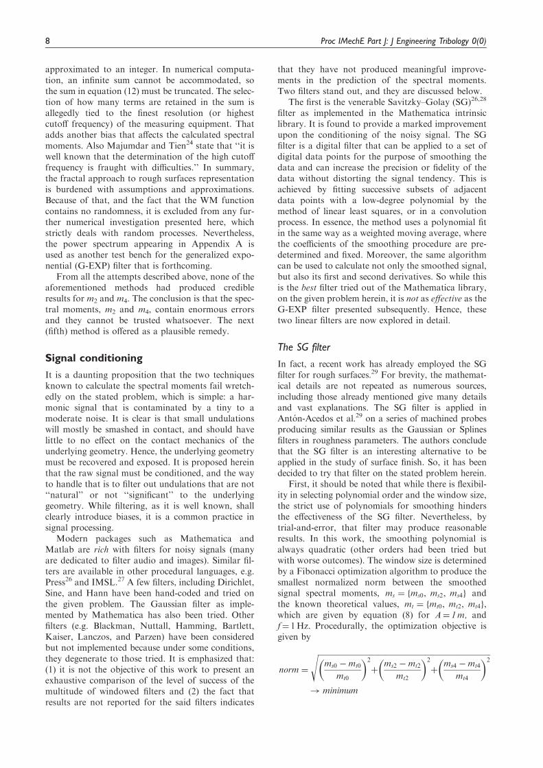
The first is the venerable Savitzky–Golay (SG)26,28

filter as implemented in the Mathematica intrinsiclibrary. It is found to provide a marked improvementupon the conditioning of the noisy signal. The SGfilter is a digital filter that can be applied to a set ofdigital data points for the purpose of smoothing thedata and can increase the precision or fidelity of thedata without distorting the signal tendency. This isachieved by fitting successive subsets of adjacentdata points with a low-degree polynomial by themethod of linear least squares, or in a convolutionprocess. In essence, the method uses a polynomial fitin the same way as a weighted moving average, wherethe coefficients of the smoothing procedure are pre-determined and fixed. Moreover, the same algorithmcan be used to calculate not only the smoothed signal,but also its first and second derivatives. So while thisis the best filter tried out of the Mathematica library,on the given problem herein, it is not as effective as theG-EXP filter presented subsequently. Hence, thesetwo linear filters are now explored in detail.

The SG filter

In fact, a recent work has already employed the SGfilter for rough surfaces.29 For brevity, the mathemat-ical details are not repeated as numerous sources,including those already mentioned give many detailsand vast explanations. The SG filter is applied inAnton-Acedos et al.29 on a series of machined probesproducing similar results as the Gaussian or Splinesfilters in roughness parameters. The authors concludethat the SG filter is an interesting alternative to beapplied in the study of surface finish. So, it has beendecided to try that filter on the stated problem herein.

First, it should be noted that while there is flexibil-ity in selecting polynomial order and the window size,the strict use of polynomials for smoothing hindersthe effectiveness of the SG filter. Nevertheless, bytrial-and-error, that filter may produce reasonableresults. In this work, the smoothing polynomial isalways quadratic (other orders had been tried butwith worse outcomes). The window size is determinedby a Fibonacci optimization algorithm to produce thesmallest normalized norm between the smoothedsignal spectral moments, ms ¼ ms0, ms2, ms4f g andthe known theoretical values, mt ¼ mt0, mt2, mt4f g,which are given by equation (8) for A¼ 1m, andf¼ 1Hz. Procedurally, the optimization objective isgiven by

norm ¼

ffiffiffiffiffiffiffiffiffiffiffiffiffiffiffiffiffiffiffiffiffiffiffiffiffiffiffiffiffiffiffiffiffiffiffiffiffiffiffiffiffiffiffiffiffiffiffiffiffiffiffiffiffiffiffiffiffiffiffiffiffiffiffiffiffiffiffiffiffiffiffiffiffiffiffiffiffiffiffiffiffiffiffiffiffiffiffiffiffiffiffims0 �mt0

mt0

� �2

þms2 �mt2

mt2

� �2

þms4 �mt4

mt4

� �2s

! minimum


Note that each term individually is normalized byits own theoretical value. That normalization guaran-tees that all moments are weighed equally (i.e. be ofsimilar significance) in the optimization process.

So first, the noisy signal, z, is smoothed by the SGfilter using the optimal window size, then derivativesare taken, and finally equations (1) to (3) are executed.Table 2 shows the same information as in Table 1, butnow this is after the SG filter is applied. It should benoted that because the SG is a linear filter, thesmoothed signal is subtracted from the raw noisysignal, leaving only the effective noise. Hence, theSNRdB can likewise be calculated according to equa-tions (10) and (11).

Figure 2 shows in red the smoothed signals for onlythe largest noise level case, �A¼ 0.3, using the intrin-sic Mathematica function, ‘‘SavitzkyGolayMatrix.’’The optimal window size found is 30. The smoothedsignal (shown in red) is compared to the raw noisysignal (shown in gray), and the pure objective signal(shown in black). Visibly, the SG filter is quite effect-ive in smoothing z(x). However, while the derivative,z’(x), generally seems to follow the objective, devi-ations from the target values are quite visible aboutthe extremum points. These deviations when summedup, according to equations (1) to (3), are responsible forthe errors in the spectral moment estimations. The big-gest problem still remains with the second derivative,z’’(x), as the deviations there are very significant, wherethe magnitudes are very far from the target. These twodeviations, and particularly the latter, cannot fullyrestore the objective spectral moments. That is apparentby inspecting the moments in Table 2 where the errorsin m2 and m4 are still quite large.

Two resolutions are also examined in Figure 2,nfft¼ 9, and nfft¼ 12 (see also Table 2). It seemsagain that as the resolution gets finer, the errors get

larger. The SG filtered signal and its derivatives(shown in red) have more difficulty following thedesired signal and its derivative (shown in black).Particularly, when the resolution is finer, nfft¼ 12,the deviations are still so enormous in the secondderivative (at least an order of magnitude largerthan the case for nfft¼ 9), necessitating dropping itfrom the figure. Even the bandwidth parameter, �,is getting worse as the resolution gets finer. The factthat the resolution issue remains unresolved is defin-itely another reason why the SG filter is still fallingshort.

In summary, while the improvements compared tothe results in Table 1 are indeed notable, however, theerrors remain at a high level, making the resultingmoments untrustworthy. Moreover, the resolutionproblem also remains unsolved because the errorsincrease with resolution refinement. In general, withthe increase of �A, the errors increase, a is deviatingquite significantly from the exact value of 1, andSNRdB decreases. It is again emphasized that this isthe best filter tried out of the Mathematica library ofintrinsic filters. So while the SG filter provides animprovement, clearly a better filter is needed. Thatfilter is the G-EXP filter that is structured next.

The G-EXP filter

The G-EXP filter shares main characteristics with theSG filter or other filters. Namely: (1) ‘‘do no harm,’’i.e. do not introduce artifacts that are not present inthe original data, and it should not distort the originaltendency or underlying geometry, (2) apply the filterin a similar way, i.e. by convolving the signal with awindowed filter, (3) preserve linearity, i.e. if the signalis a total of two or more data sets, then the overallfiltered effect can be obtained by superposition of the

Table 2. Results using the SG filter.

At �A ¼ 0

m0¼ 1/2¼ 0.5 m2 ¼ 2�2 ¼ 19:739 m4 ¼ 8�4 ¼ 779:27

�¼ 1 SNRdB ¼ 1Value Error% Value Error% Value Error%

nfft¼ 9, �x ¼ 0:01227

�A ¼ 1% 0.500 0.0 19.66 0.4 854.25 9.52 1.11 52.2

�A ¼ 10% 0.474 5.2 18.93 4.11 1950.0 150.2 2.58 36.1

�A ¼ 30% 0.417 16.6 16.75 15.2 5644.0 624.3 8.39 28.0

nfft¼ 11, �x ¼ 0:00307

�A ¼ 1% 0.499 0.2 19.67 0.4 1505.0 93.2 1.94 57.25

�A ¼ 10% 0.465 6.9 18.61 5.72 1.626E4 1987 21.85 40.28

�A ¼ 30% 0.387 22.7 15.36 22.2 6.801E4 8628 111.39 32.37

nfft¼ 12, �x ¼ 0:001534

�A ¼ 1% 0.500 0.0 19.65 0.45 3107.9 298.8 4.0 60.03

�A ¼ 10% 0.450 9.6 18.06 8.52 4.958E4 6.26E3 68.75 44.0

�A ¼ 30% 0.330 34.78 12.88 34.77 1.935E5 2.47E4 380.6 35.68

SG: Savitzky–Golay.

Notes: Values of the exact spectral moments and their numerically calculated values with relative errors for various noise amplitudes, �A, and

resolutions, �x. Given also are the bandwidth parameter, �, and the signal to noise ratio in (dB). For all cases, A¼ 1 m and f¼ 1 Hz.

Green 9

data sets filtered individually; and, vice versa, subtrac-tion a certain filtered data set from the filtered total,would reveal the remainder intact, and (4) similar tothe aforementioned filters, it should contain coeffi-cients or weights that are symmetric about the mid-point. That is a necessity as there should not bepreference to neighboring points on either side of apoint of interest undergoing smoothing.

On the other hand, the G-EXP filter is significantlydifferent from the SG filter in some major ways. TheSG filter uses polynomials of fixed order with fixedcoefficients (i.e. fixed windowed weights), while theG-EXP filter is flexible using any positive real param-eters, allowing the weights to assume whicheverdesigned values.

The G-EXP filter can be thought of belonging to ageneral exponential form

g xð Þ ¼ e��jxjn

@ x 2 �L,Lð Þ ð13Þ

This generalization allows for a three-parameter filterdesign where the power, n, can take on any positive real

value. A changeable power, n, provides a whole family ofexponential filters. The absolute of jxj allows the powercalculation, while preserving filter symmetry for anypower, n. If n¼ 0, then g(x) degenerates to a Dirichletfilter. When n¼ 1, then g(x) is strictly exponential, andwhen n¼ 2, then g(x) is related to the standard normaldistribution,30–32 retaining only the quadratic exponentialform (The standard normal distribution is: P xð Þ ¼1=

ffiffiffiffiffiffi2�p� �

e�x2=2 @x 2 �1,1ð Þ. First, the leading coef-

ficient of 1=ffiffiffiffiffiffi2�p

is of no consequence, because the G-EXP filter as given subsequently by equation (14) is nor-malized. Then, the parameter � is free to take on anypositive real value (i.e. other than ½). Finally, the rangex 2 �L,Lð Þ, i.e. the filter window size, is selectable oradjustable.), in which case the absolute of x can beomitted. The filter is actually completely stated by

g ¼ e��jRange �L,L½ �jn=Total e��jRange½�L,L�jn

ð14Þ

In the current work, n¼ 1 and n¼ 2 are tried, andfound to smooth the signals as intended. However,because of the superior results rendered by the filter

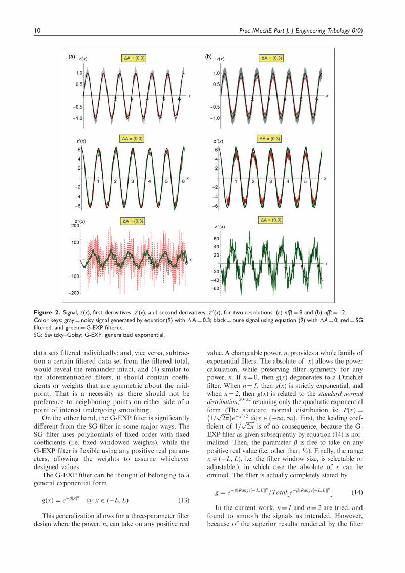
Figure 2. Signal, z(x), first derivatives, z0(x), and second derivatives, z00(x), for two resolutions: (a) nfft¼ 9 and (b) nfft¼ 12.

Color keys: gray¼ noisy signal generated by equation(9) with �A¼ 0.3; black¼ pure signal using equation (9) with �A¼ 0; red¼ SG

filtered; and green¼G-EXP filtered.

SG: Savitzky–Golay; G-EXP: generalized exponential.


with n¼ 2, other values of n had been bypassed.Hence, for the remainder of this work, the G-EXPis specific to the case of n¼ 2. In which case, equation(13) degenerates to

g xð Þ ¼ e��x2

@ x 2 �L,Lð Þ ð13� aÞ

So now, the G-EXP filter has two parameters leftthat can be adjusted. Specifically, the tuning param-eter, �, is any real positive value, while the integer, L,decides the window size. Again, using Mathematica’ssyntax, the G-EXP filter, given in equation (14), isentirely expressed by a single statement

g ¼ e��Range �L,L½ �2=Total e��Range½�L,L�2

h ið14� aÞ

The advantage of the G-EXP filter is that L and � aregenerally not restricted, and in addition to n, they allowfor a ‘‘three-degree of freedom’’ filter. The only restric-tion on L is that it is sufficiently smaller than the numberof points in the signal to be smoothed, i.e. L<<N,which should commonly be the case. Additional con-struction details of the G-EXP filter, along with exam-ples, are given in Appendix C. For portability, theappendix provides also a Fortran 77 code for the con-struction and execution of the G-EXP filter.

We turn now to the outcomes of applying theG-EXP filter. As described above, similar to the appli-cation of the SG filter, a Fibonacci optimization algo-rithm is executed to assist in the parameter selection.The process is to try a set of window sizes, L, and thenlet the optimization algorithm determine the optimal� for each one of them. Of all sets of L and �, the onethat produces the smallest normalized norm betweenthe smoothed signal spectral moments and the known

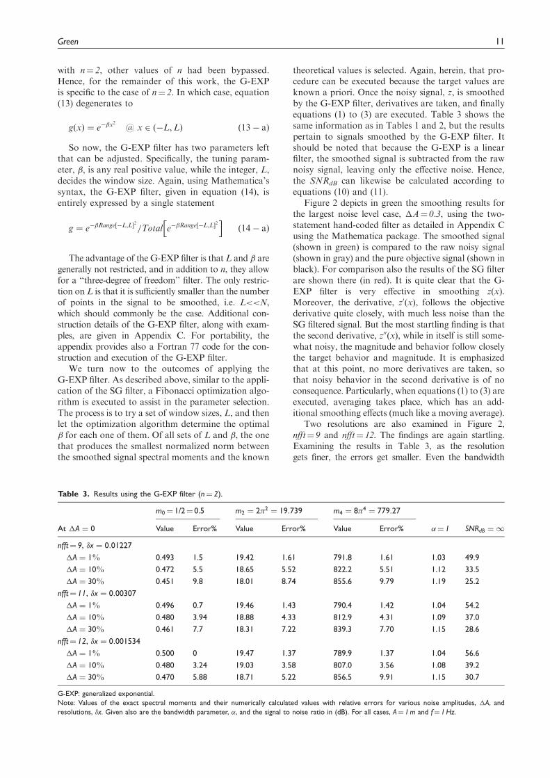
theoretical values is selected. Again, herein, that pro-cedure can be executed because the target values areknown a priori. Once the noisy signal, z, is smoothedby the G-EXP filter, derivatives are taken, and finallyequations (1) to (3) are executed. Table 3 shows thesame information as in Tables 1 and 2, but the resultspertain to signals smoothed by the G-EXP filter. Itshould be noted that because the G-EXP is a linearfilter, the smoothed signal is subtracted from the rawnoisy signal, leaving only the effective noise. Hence,the SNRdB can likewise be calculated according toequations (10) and (11).

Figure 2 depicts in green the smoothing results forthe largest noise level case, �A¼ 0.3, using the two-statement hand-coded filter as detailed in Appendix Cusing the Mathematica package. The smoothed signal(shown in green) is compared to the raw noisy signal(shown in gray) and the pure objective signal (shown inblack). For comparison also the results of the SG filterare shown there (in red). It is quite clear that the G-EXP filter is very effective in smoothing z(x).Moreover, the derivative, z0(x), follows the objectivederivative quite closely, with much less noise than theSG filtered signal. But the most startling finding is thatthe second derivative, z00(x), while in itself is still some-what noisy, the magnitude and behavior follow closelythe target behavior and magnitude. It is emphasizedthat at this point, no more derivatives are taken, sothat noisy behavior in the second derivative is of noconsequence. Particularly, when equations (1) to (3) areexecuted, averaging takes place, which has an add-itional smoothing effects (much like a moving average).

Two resolutions are also examined in Figure 2,nfft¼ 9 and nfft¼ 12. The findings are again startling.Examining the results in Table 3, as the resolutiongets finer, the errors get smaller. Even the bandwidth

Table 3. Results using the G-EXP filter (n¼ 2).

At �A ¼ 0

m0¼ 1/2¼ 0.5 m2 ¼ 2�2 ¼ 19:739 m4 ¼ 8�4 ¼ 779:27

�¼ 1 SNRdB ¼ 1Value Error% Value Error% Value Error%

nfft¼ 9, �x ¼ 0:01227

�A ¼ 1% 0.493 1.5 19.42 1.61 791.8 1.61 1.03 49.9

�A ¼ 10% 0.472 5.5 18.65 5.52 822.2 5.51 1.12 33.5

�A ¼ 30% 0.451 9.8 18.01 8.74 855.6 9.79 1.19 25.2

nfft¼ 11, �x ¼ 0:00307

�A ¼ 1% 0.496 0.7 19.46 1.43 790.4 1.42 1.04 54.2

�A ¼ 10% 0.480 3.94 18.88 4.33 812.9 4.31 1.09 37.0

�A ¼ 30% 0.461 7.7 18.31 7.22 839.3 7.70 1.15 28.6

nfft¼ 12, �x ¼ 0:001534

�A ¼ 1% 0.500 0 19.47 1.37 789.9 1.37 1.04 56.6

�A ¼ 10% 0.480 3.24 19.03 3.58 807.0 3.56 1.08 39.2

�A ¼ 30% 0.470 5.88 18.71 5.22 856.5 9.91 1.15 30.7

G-EXP: generalized exponential.

Note: Values of the exact spectral moments and their numerically calculated values with relative errors for various noise amplitudes, �A, and

resolutions, �x. Given also are the bandwidth parameter, �, and the signal to noise ratio in (dB). For all cases, A¼ 1 m and f¼ 1 Hz.

Green 11

parameter, �, is getting better as the resolution gets finer,being very close to the ideal value of 1. The SNRdB isalso better compared to those reported in Tables 1 and 2.

In summary, the G-EXP filter makes a remarkablediscovery of the underlying geometry of the puresignal. The filter recovers almost to perfection theideal spectral moments and the bandwidth parameter.There is no longer a resolution problem, in fact, as theresolution gets finer, the results get better. All this istrue for tiny, moderate, and fairly large magnitudes ofnoise, �A. The SNRdB increases to acceptable values.It can be concluded that the G-EXP filter provides avery effective solution for noisy signals.

In addition to that objective, the G-EXP filter isshown to be a general tool for smoothing out noisysignals not only in the time domain but also in thefrequency domain. The latter capability is demon-strated by the green color line in Figure 3 inAppendix A, where the G-EXP filter is successfullyused to smooth out also the power spectrum.Moreover, the G-EXP filter can be applied repeatedlyin what is known as ‘‘passes.’’ Each pass tends toremove even more noise, exposing more of the under-lying signal. For some filters (e.g. the G-EXP), theprocess removes the noise very effectively even byusing a single pass. But like other filters, additionalpasses may increase the possibility of signal distor-tion, loss of information, and more importantly, Lpoints on each side of the signal are lost after eachpass. That is, N must be much greater than L. In thiswork, only one pass is applied to test the various fil-ters without the bias of repeated passes.

Application of the G-EXP filter on realand fractal rough surfaces

The challenge in calculating the spectral moments forreal surfaces stems from the fact that the target valuesare not known a priori. A trial-and-error process isneeded to find the filter parameters. The G-EXP filter,with L¼ 20, and �¼ 5, is used upon two real roughsurfaces of a ceramic spherical indenter loaded againsta multi-wall carbon nanotube counterpart.20 TheGW1 model is subsequently executed. For brevity,details of that application and measuring techniquesare spared. The important and relevant fact herein isthat the roughness of each surface is 3D, not homo-geneous, and not isotropic. The said paper20 detailshow such surface characteristics are handled by pur-suing McCool’s6 procedure. That involves finding setsof two two-dimensional (2D) orthogonal directionsof maximum and minimum spectral moments thatare averaged either arithmetically or harmonically.Hence, the procedure developed herein for a 2D caseis specifically suitable to handle 3D surface roughness.It is not the intent herein to repeat the calculationprocedure other than to exhibit how the G-EXP isapplied to such 2D rough surfaces, as shown inFigure 3. As can be seen, some of the data of the

original signal measurements are exceedingly far offfrom the ‘‘norm.’’ These are either defects in the sur-faces, voids or bumps in the material, or they areequipment related, producing erroneous measure-ments. Should the original data are taken ‘‘as is’’ tocalculate the spectral moments according to equations(1) to (3), enormous errors would result, as it takes onlyone ‘‘bad’’ point, or a region of ‘‘bad’’ points to skewthe results very profoundly. Filtering out those datapoints that ‘‘do not belong’’ is undoubtedly essential.

The G-EXP filter can be applied equally well alsoto surface having fractal roughness. That, however, isnot necessary, as fractal roughness contains no noise.As discussed above, the signal is entirely deterministicfor given A, D, and �. Consider equation (12) mod-ified to have a truncated sum having an upper sum-mation bound, n2

z xð Þ ¼ AðD�1ÞXn2n¼n1

cos 2��nx

�ð2�DÞn15D5 2,

�4 1, n25n1

The value of n2 is related to the finest resolution(i.e. highest frequency) capability of the measuringequipment.24 The signal would appear ‘‘smooth’’ or‘‘rough’’ depending on how ‘‘small’’ or ‘‘large’’ is n2,respectively. Hence, reducing the value of n2 smooth-ens the signal mathematically without filtering.Fractal roughness deserves a completely differenttreatment that is beyond the scope of this work.

Conclusions

The upside of the GW model is that only three spectralmoments are needed to execute it. That is also the down-side of the GW model, as not too many parameters areavailable to work with. To estimate the spectralmoments reliably, the surface roughness needs toundergo massive data reduction. So, the estimationmust be quite good with almost zero room for error.

In the current work, a sine waveform is contami-nated by a white noise process varying in magnitudefrom tiny to moderate. To recover the underlyinggeometry, these methods have been tested to calculatethe spectral moment: (1) finite-difference derivativesusing accurate five-points (instead of two- or three-points as suggested by McCool), (2) data partitioningand averaging (to reduce statistical errors), (3) calcu-lation of derivatives via interpolation functions, and(4) calculation via the power spectrum. The followingconclusions can be drawn:

1. The finite difference method as suggested byMcCool to calculate the spectral moments failsdramatically on his own problem when the wave-form is contaminated even by the tiniest noise, andmatters become worse with moderate to highernoise levels.


2. The zeroth spectral moment does not containderivatives in its definition and, hence, it is lesssensitive to noises in the signal, i.e. its predictionby equation (1) is quite good and can be trusted.

3. The second spectral moment depends on the firstderivative, and hence a noisy signal affects itsaccuracy because derivatives tend to accentuateerrors.

4. The fourth spectral moment depends on thesecond derivative (theoretically, it is the derivativeof the first derivative, which is already erroneous,although herein it is calculated directly by a five(5) finite difference, without resorting to a ‘‘deriva-tive of the first derivative’’). The errors in the cal-culation of the fourth spectral moment are muchworse than even the second moment.

5. A finer resolution makes things even worse, but thatis attributed to the presence of the noise. Once thenoise is attenuated, a higher resolution producesbetter predictions for the spectral moments.

6. Signal conditioning is a necessity for the removalof noise in the data. Various filters have been tried,but most have not greatly improved upon the cal-culation of the spectral moments. The venerableSG filter is found to make progress in that calcu-lation, but still the results are objectionable.

7. The only filter that is successful in restoring theunderlying geometry and removing the noiseeffectively (even when it is of a relatively high mag-nitude) is the G-EXP filter. Upon smoothing, thepredictions of the spectral moments and the band-width parameter are extremely close to the theor-etical values. The SNR improves considerablyupon the application of the G-EXP filter.

8. The G-EXP is applied upon real surfaces in eightdifferent directions, and it is shown to smoothedout the enormous noise levels very effectively.

9. The G-EXP filter can be applied not only on thewaveform, but also on the power spectrum.

10. The G-EXP filter is a linear filter and, hence,superposition can be applied and taken advantageof so that the noise can be isolated.

11. The G-EXP can be applied in successive passes, ifdeemed necessary.

Declaration of Conflicting Interests

The author(s) declared no potential conflicts of interest with

respect to the research, authorship, and/or publication ofthis article.

Funding

The author(s) received no financial support for the research,authorship, and/or publication of this article.

References

1. Greenwood JA and Williamson JBP. Contact of nomin-ally flat surfaces. Proc R Soc London Ser A. Math PhysSci 1966; 295: 300–319.

2. Jackson RL and Green I. On the modeling of elasticcontact between rough surfaces. Tribol Trans 2011; 54:300–314.

3. Chang WR, Etsion I and Bogy DB. An elastic-plasticmodel for the contact of rough surfaces. J Tribol 1987;109: 257.

4. Jackson RL and Green I. A statistical model of elasto-plastic asperity contact between rough surfaces. TribolInt 2006; 39: 906–914.

5. Kogut L and Jackson RL. A comparison of contactmodeling utilizing statistical and fractal approaches.J Tribol 2006; 128: 213.

6. McCool JI. Relating profile instrument measurements

to the functional performance of rough surfaces.J Tribol 1987; 109: 264.

7. McCool JI. Finite difference spectral moment estima-

tion for profiles the effect of sample spacing and quant-ization error. Precis Eng 1982; 4: 181–184.

8. Sweitzer K, Bishop N and Genberg V. Efficient

Computation of Spectral Moments for Determinationof Random Response Statistics. In: Proceedings ofISMA 2004, Signal Processing and Instrumentation,

2004, pp. 2677–2691.9. Davidson KL and Loughlin PJ. Instantaneous spectral

moments. J Franklin Inst 2000; 337: 421–436.10. Vogel F. Spectral moments and linear models used for

photoacoustic detection of crude oil in produced water,Department of Informatics, University of Oslo, Oslo,Norway, 2001.

11. Brown SR. Simple mathematical model of a rough frac-ture. J Geophys Res: Solid Earth 1995; 100: 5941–5952.

12. Bendat JS and Piersol AG. Measurement and analysis of

random data. New York, NY: Wiley, 1966.13. Bendat JS and Piersol AG. Engineering applications of

correlation and spectral analysis. New York, NY: JohnWiley and Sons, Inc., 1980.

14. Bendat JS and Piersol AG. Random data: analysis andmeasurement procedures. Hoboken, NJ: John Wiley &Sons, 2011.

15. Pawar G, Pawlus P, Etsion I, et al. The effect of deter-mining topography parameters on analyzing elasticcontact between isotropic rough surfaces. J Tribol

2012; 135: 011401.16. Xu Y and Jackson RL. Statistical models of nearly com-

plete elastic rough surface contact – comparison with

numerical solutions. Tribol Int 2017; 105: 274–291.

17. Kalin M, Pogacnik A, Etsion I, et al. Comparing sur-

face topography parameters of rough surfaces obtainedwith spectral moments and deterministic methods.Tribol Int 2016; 93: 137–141.

18. Nayak PR. Random process model of rough surfaces.J Lubr Technol 1971; 93: 398–407.

19. Bhushan B. Surface roughness analysis and measurementtechniques. Modern tribology handbook, two volume set.Boca Raton, FL: CRC Press, 2000.

20. Reinert L, Green I, Gimmler S, et al. Tribologicalbehavior of self-lubricating carbon nanoparticle rein-forced metal matrix composites. Wear 2018; 408: 72–85.

21. Hildebrand FB. Introduction to numerical analysis.

New York: McGraw-Hill, 1974.22. Pogacnik A and Kalin M. How to determine the

number of asperity peaks, their radii and their heightsfor engineering surfaces: a critical appraisal.Wear 2013;

300: 143–154.

Green 13

23. Hariri A, Zu JW and Mrad RB. N-point asperity modelfor contact between nominally flat surfaces. J Tribol2006; 128: 505–514.

24. Majumdar A and Tien CL. Fractal characterization andsimulation of rough surfaces. Wear 1990; 136: 313–327.

25. Berry MV and Lewis ZV. On the Weierstrass–Mandelbrot

fractal function. Proc R Soc A 1980; 370: 459–484.26. Press WH, ed., FORTRAN numerical recipes. Cambridge,

UK; New York, NY: Cambridge University Press, 1996.

27. IMSL. STAT/Library: FORTRAN subroutines forstatistical analysis: user’s manual. Houston, TX:IMSL, Inc., 1987.

28. Savitzky A and Golay MJE. Smoothing and differenti-

ation of data by simplified least squares procedures.Anal Chem 1964; 36: 1627–1639.

29. Anton-Acedos P, Sanz-Lobera A, Lopez-Baos A, et al.

Feasibility analysis of Savitzky-Golay filter implemen-tation in surface texture filtering and measurement.Procedia Manuf 2017; 13: 503–510.

30. Kenney JF. Mathematics of statistics. New York, NY:Van Nostrand, 1964.

31. Weisstein E. Standard normal distribution – from

Wolfram MathWorld (Online), http://mathworld.wolf-ram.com/StandardNormalDistribution.html (accessed10 May 2019).

32. Abramowitz M and Stegun IA. National Bureau of

Standards: applied mathematics series. vol. 55.Gaithersburg, MD: National Bureau of Standards,1972, p.1060.

Appendix A. The spectral moments viathe power spectrum

If the procedure for obtaining the spectral moments isproblematic using numerical differentiation, perhapsusing equation (4) on noisy signals can produce adesirable solution. So, the next step is to obtain thepower spectrum of the signal investigated herein. It isnoted the noise is superimposed upon the waveform.Thus, according to equation (9), we have a signal of

z xð Þ ¼ A sin 2�fxð Þ þ noise½ �A¼1, f¼1¼ sin wxð Þ þ noise

ð15Þ

where noise is a random process as discussed above.Note that w¼ 2�, is the specific frequency of thewaveform of equation (5). The power spectrum isdefined by the Fourier transform for a continuousfunction

Z !ð Þ ¼

Z 1�1

z xð Þe�2�ix! dx ð16Þ

where here, and in equation (4), ! is a general fre-quency in the entire spectrum, i.e. ! 2 �1,1½ �.Since the Fourier transform is a linear operator,and had z(x) in equation (12) been a continuous func-tion then

Z !ð Þ ¼ Z wxð Þ þ Z noiseð Þ ð17Þ

However, the noise herein is a white noise processwith a uniform distribution. By definition, its Fouriertransform is ‘‘flat’’ and equals to zero, i.e. Z(noise)¼ 0throughout the entire spectrum regardless of the ampli-tude �A (see equation (9)). That leaves

Z !ð Þ ¼ Z wxð Þ ¼ iffiffiffiffiffiffiffiffi�=2

p� !� wð Þ � � !þ wð Þ½ �

ð18Þ

where �(*) is the Dirac delta function. The power ofthe signal is

P !ð Þ ¼ Z !ð Þ�� 2¼ �=2ð Þ � !� wð Þ � � !þ wð Þ½ �

2

¼ �=2ð Þ �2ð!� wÞ � 2� !� wð Þ� !þ wð Þ

þ �2 !þ wð Þ

ð19Þ

Indeed, the discussion can be limited to just posi-tive frequencies ! 2 ½0,1�. This result for the powerneeds to be substituted in equation (4) to calculate thespectral moments k¼ 0, 2, 4. However, when equation(19) is substituted in equation (4), an exact mathema-tical solution for the latter is elusive. That mathema-tical difficulty compelled the workarounds andapproximations made by Majumdar and Tien.24,25

Those workarounds contain biases and the approxi-mated moments cannot be regarded exact solutions.

To further illustrate the difficulty with the spectrumapproach, a numerical fast Fourier transform (FFT)is executed upon the discrete values of the contami-nated signal of z(x) (given by equation (9)). The powerspectrum is obtained, and the spectral moments (fol-lowing equation (4)) are calculated numerically usingeither a trapezoidal or the Simpson rule (both givingvery similar results). That approach is tried for thenoise level case of �A¼ 30%, and nfft¼ 9, wherethe power spectrum is shown in Figure 4. While thespectrum captures well the specific dominant fre-quency of the waveform (see the peak at f¼ 1 or!¼w¼ 2�), the final results for {m0, m2,m4}¼ {0.5012, 149.2, 7.466E6} are inconsequential.First, the power spectrum shown in Figure 3 cannotrepresent the exact solution that equation (19) com-mands. Second, results for m2 and m4 are in greaterror and intolerable (similar or even worse thanthose appearing in Table 1).

Appendix B. Numerical derivatives

For simplicity, a three-point central derivative will beused to show the reason for the increasing error in thecomputation of m2 and m4. Starting off with the firstderivative (omitting the truncation error),

z0 xð Þ ¼z xþ �xð Þ � z x� �xð Þ

2�xð20Þ

Theoretically, for A¼ 1 and f¼ 1, at x¼ k/4 fork¼ 1, 3, 5. . ., the derivative of equation (5) equals


zero. Indeed, when the pure equation (5) is digitizeddiscretely, z x� �xð Þ ¼ z xþ �xð Þ at the said points,and the numerical derivative turns out the correctzero result. However, using equation (20) on thenoisy z(x) at those points, z x� �xð Þ 6¼ z xþ �xð Þ

because of the added random noise, thus clearly

rendering a result that is not zero. That phenomenonhappens not only at the selected x values, but actuallyat any value of x2{0, xmax} along the signal. As noiseis modulated by �A, then when the sum is employedon (z’(x))2 according to equation (2), the accumula-tion of the error only intensifies.

Figure 3. Real rough surfaces from Reinert et al.20 Abscissa and ordinate are shown in m. (a) Composite carbon nanotube and

(b) Ceramic ball counterpart.

Color key: Orange¼ the original rough surfaces, purple¼ the G-EXP smoothed surfaces, with L¼ 20 and �¼ 5.

Source: reproduced with permission from Reinert et al. 2018.20


Green 15

The second central numerical derivative is

z00 xð Þ ¼z x� �xð Þ � 2z xð Þ þ z xþ �xð Þ

�x2

¼z xþ �xð Þ � z xð Þ½ � � z xð Þ � z x� �xð Þ½ �

�x2

¼z xþ �xð Þ � z xð Þ½ �=�x� z xð Þ � z x� �xð Þ½ �=�x

�xð21Þ

The second form of equation (21) emphasizesthat the second derivative (like the first derivative) isbased on the difference of the differences betweenthe neighboring z(x) values, while the third form ofthe equation renders the expected result that thesecond derivative is, of course, a derivative of the firstderivative. Hence, if the first derivative contains errorsclearly, the second derivative must be erroneous too.

So again, theoretically, for A¼ 1 and f¼ 1, atx¼ k/4 for k¼ 0, 2, 4. . .N when the digitized puresignal of equation (5) is used, the numerical secondderivative equals identically zero, as it should be.However, when the noisy z(x) values are substitutedinto equation (21), the results are not zero. And asexplained above, that behavior happens actually atany value of x2{0, xmax} along the signal. And asthe error is modulated by �A, then when the sum isexecuted on (z00(x))2 according to equation (3), theaccumulation of the error escalates dramatically.

The analysis above holds for any central differenceof any order, including order five (5) that is usedherein. The conclusion is that for m0, which doesnot include derivatives in its definition, the estimationby equation (1) can be considered ‘‘correct’’ or ‘‘suffi-ciently accurate’’ as the noise contaminates the mag-nitude of the signal, but if the noise amplitude isrelatively small, then m0 shall have only a correspond-ing small error. However, m2 and m4 depend on thederivatives, which happen on the differences betweenz(x) values (so the relative magnitudes of z(x) valuesthemselves are irrelevant). Hence, the errors in thederivatives are directly proportional to the magnitude

of the noise, and that cannot be mitigated. In otherwords, m0 hinges on ‘‘macro’’ or ‘‘global’’ quantitieswhere the noise effects are less significant, while m2

and m4 hinge on ‘‘micro’’ or ‘‘local’’ quantitieswhere the noise effects are very significant.

Appendix C. The construction of theG-EXP filter

The filter is best explained along with an example. Thefilter is defined by equation (13)

g xð Þ ¼ e��jxjn

@ x 2 �L,Lð Þ; x ¼ Range �L,L½ �

ð13Þ

Suppose that L¼ 3, then using a Mathematicastatement: x¼Range [–L, L] results in a vector{x}¼ {–3, –2, –1, 0, 1, 2, 3}. Here, the vector {x}has no physical meaning; it is a dummy list (or aservice vector) of length of 2Lþ 1, and it is used forillustration only. If also n¼ 2, and �¼ 0.5, then uponsubstitution into equation (13), we have

g� �¼ 0:0111, 0:1353, 0:6065, 1:, 0:6065,f

0:1353, 0:0111g

Clearly, by definition, the vector {g} also has anodd length, 2Lþ 1. The values it contains are sym-metric about the center point. These values have therole of weights, where the center weight has the largestvalue. The next step is to ensure that the smoothedsignal does not overshoot, i.e. worsen the signal.Hence, the vector {g} is normalized by its total, sothat the largest central weight equals to 1/Total[g].Hence, issuing the computer assignment

g ¼ g=Total g½ � ð22Þ

achieves that goal. Instead of the two computerassignments expressed by equations (13) and (22),the filter design is reduced to a single Mathematicastatement, as given by equation (14)

g ¼ e��jRange �L,L½ �jn=Total e��jRange �L,L½ �jn

ð14Þ

The numerator of equation (14) contains a list,which is normalized by its own total, and it isalways symmetric about the origin. Clearly, thedummy variable ‘‘x’’ disappeared, because it is imma-terial for the formal filter design, but it has utility forillustration purposes. Therefore, the filter given byequation (14) contains a list of weights that total tothe value of one unit. On the said example, we have

g� �¼ g� �

=Total g½ �

¼ 10�3 � 4:43305, 54:0056, 242:036,f

399:05, 242:036, 54:0056, 4:43305g

Figure 4. Power spectrum for a sine waveform contaminated

by a white noise level of �A¼ 30%, shown in blue color.

A smoothed spectrum is shown in green.


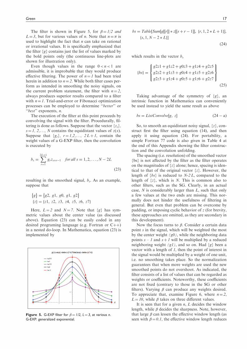
The filter is shown in Figure 5, for �¼ 1/2 andL¼ 3, but for various values of n. Note that n¼� isused to highlight the fact that n can take on rationalor irrational values. It is specifically emphasized thatthe filter {g} contains just the list of values marked bythe bold points only (the continuous line-plots areshown for illustration only).

Even though values in the range 0< n< 1 areadmissible, it is improbable that they would produceeffective filtering. The power of n¼ 1 had been triedherein in addition to n¼ 2. While both filter cases per-form as intended in smoothing the noisy signals, onthe current problem statement, the filter with n¼ 2,always produces superior results compared to a filterwith n¼ 1. Trial-and-error or Fibonacci optimizationprocesses can be employed to determine ‘‘better’’ or‘‘best’’ exponents, n.

The execution of the filter at this point proceeds byconvolving the signal with the filter. Procedurally, fil-tering is done as follows. Suppose that the vector {zs},s¼ 1, 2,. . ., N contains the equidistant values of z(x).Suppose that {gr}, r¼ 1,2,. . ., 2 Lþ 1, contain theweight values of a G-EXP filter, then the convolutionis executed by

bs ¼X2Lþ1r¼1

grzsþr�1 for all s ¼ 1, 2, . . . ,N� 2L

ð23Þ

resulting in the smoothed signal, bs. As an example,suppose that

g� �¼ g2, g1, g0, g1, g2� �

zf g ¼ z1, z2, z3, z4, z5, z6, z7f g

Here, L¼ 2 and N¼ 7. Note that {g} has sym-metric values about the center value (as discussedabove). Equation (23) can be easily coded in anydesired programing language (e.g. Fortran or Cþþ)in a nested do-loop. In Mathematica, equation (23) isimplemented by

bs ¼ Table Sum g r½ �½ � � z sþ r� 1½ �½ �, r, 1, 2 � Lþ 1f g½ �;½

s, 1,N� 2 � Lf g�

ð24Þ

which results in the vector bs

bsf g ¼

g2z1þ g1z2þ g0z3þ g1z4þ g2z5



8><>:

9>=>;ð25Þ

Taking advantage of the symmetry of {g}, anintrinsic function in Mathematica can convenientlybe used instead to yield the same result as above

bs ¼ ListConvolve g, z½ � ð24� aÞ

So, to smooth an equidistant noisy signal, {z}, con-struct first the filter using equation (14), and thenapply it using equation (24). For portability, asimple Fortran 77 code is also given in Table 4 atthe end of this Appendix showing the filter construc-tion and the convolution unfolding.

The spacing (i.e. resolution) of the smoothed vector{bs} is not affected by the filter as the filter operateson the magnitudes of {z} alone; hence, spacing is iden-tical to that of the original vector {z}. However, thelength of {bs} is reduced to N-2L, compared to thelength of {z}, which is N. This is common also toother filters, such as the SG. Clearly, in an actualcase, N is considerably larger than L, such that onlya few values at the two ends are missing. This nor-mally does not hinder the usefulness of filtering ingeneral. But even that problem can be overcome bypadding, or imposing cyclic behavior of z (for brevity,these approaches are omitted, as they are secondary inthis development).

Now the focus turns to �. Consider a certain datapoint s in the signal, which will be weighted the mostby the center weight (g0), while the neighboring datapoints s – 1 and sþ 1 will be multiplied by a reducedneighboring weight (g1), and so on. Had {g} been avector with a length of 1, then the point of interest inthe signal would be multiplied by a weight of one unit,i.e. no smoothing takes place. So the normalizationguarantees that when more weights are used the newsmoothed points do not overshoot. As indicated, thefilter consists of a list of values that can be regarded asweights or coefficients. Noteworthy, these coefficientsare not fixed (contrary to those in the SG or otherfilters). Varying � can produce any weights desired.To appreciate that, examine Figure 6, where n¼ 2,L¼ 10, while � takes on three different values.

It is seen that for a given n, L decides the windowlength, while � decides the sharpness. Note, however,that large � can lessen the effective window length (asseen with �¼ 0.1, the effective window length reduces

Figure 5. G-EXP filter for �¼ 1/2, L¼ 3, at various n.


Green 17

to 6 because at point 7 and above, the {g} valuesapproach zero on both ends). So while the two para-meters L and � provide great flexibility in the filterdesign, a meticulous trial-and-error process is nor-mally entailed in their selection. The general trendsare: as L gets larger, more neighboring points partici-pate in the smoothing, where a larger � puts moreweight on the closest neighbors and the extent ofsmoothing is reduced (and vice versa for smallervalues of L and �). Clearly L should be sufficientlysmaller than the number of data points, N, to besmoothed.

Table 4. A Fortran 77 code to produce and execute the

G-EXP filter for the example above.

parameter (n¼ 7, L¼ 2, ng¼ 2*Lþ 1, nb¼ n-2*L)

dimension g(ng), z(n), bs(nb)

data z/1.,2.,3.,4.,5.,6.,7./

data beta/0.5/

write(6,*) ‘‘Construct the filter as in equation (13)’’

sum¼ 0.0

do i¼ 1,ng

x¼ i-(ngþ 1)/2

g(i)¼ exp(-beta*x**2)

sum¼ sumþ g(i)

write(6,*) i,’ ‘,x, ‘ ‘, g(i)

enddo

write(6,*) ‘‘Normalize the filter as in equation (22)’’

do i¼ 1,ng

g(i)¼ g(i)/sum

write(6,*) i,’ ‘,g(i)

enddo

write(6,*) ‘‘Execute the convolution given

in equation (24) or (24-a)’’

do is¼ 1,nb

bs(is)¼ 0.0

do ir¼ 1,2*Lþ 1

bs(is)¼ bs(is)þ g(ir)*z(isþ ir-1)

enddo

write(6,*) is,’ ‘,bs(is)

enddo

write(6,*)’Verify results expected (in paper): for L¼ 2 and any

n’

do is¼ 1,nb

i¼ is-1

write(6,*) is,’ ‘,

g(1)*z(1þ i)þ g(2)*z(2þ i)þ g(3)*z(3þ i)þ

g(4)*z(4þ i)þ g(5)*z(5þ i)

enddo

end


Figure 6. The G-EXP filter for n¼ 2, L¼ 10, and three values

of �.



metrology and numerical characterization of random rough

Documents