IN DEGREE PROJECT MECHANICAL ENGINEERING,SECOND CYCLE, 30 CREDITS

, STOCKHOLM SWEDEN 2020

Methods to Predict Hull Resistance in the Process of Designing Electric Boats

ELIN LINDBERGH

FELICIA AHLSTRAND

KTH ROYAL INSTITUTE OF TECHNOLOGYSCHOOL OF ENGINEERING SCIENCES

Methods to Predict Hull Resistance in the Process of Designing Electric BoatsSwedish title: Metoder for att Uppskatta Skrovmotstandet i Designprocessen for Elektriska Batar

ELIN LINDBERGH, FELICIA AHLSTRAND

TRITA: TRITA-SCI-GRU 2020:185

Degree Project in Naval Architecture, Second Cycle, 30 creditsCourse SD271XStockholm, Sweden, 2020

Supervisors: Hans Liwang, KTHJohannes Roselius, X Shore

Examiner: Jakob Kuttenkeuler, KTH

Center for Naval ArchitectureSchool of Engineering SciencesKTH Royal Institute of TechnologySE-100 44, StockholmSwedenTelephone: +46 8 790 60 00

Host company: X Shore

AbstractCombustion engines in boats cause several environmental problems, such as greenhouse gas emis-sions and acidification of oceans. Most of these problems can be reduced by replacing the com-bustion engines with electric boats. The limited range is one of the main constraints for electricboats, and in order to decrease the energy consumption, applicable resistance prediction methodsare necessary in the hull design process. X Shore, which is a start-up company in the electric boatsector, lacks a systematic way of predicting resistance in an early design phase.

In this study, four well-known methods - CFD, Holtrop & Mennen, the Savitsky method andmodel test - have been applied in order to predict resistance for a test hull. The study is limitedto bare hull resistance and calm water conditions. CFD simulations are applied using the softwareANSYS FLUENT 19.0. The simulations were based on the Reynolds Average Navier-Stokes equa-tions with SST k-ω as turbulence model together with the volume of fluid method describing thetwo-phased flow of both water and air surrounding the hull. The semi-empirical methods, Holtrop& Mennen and the Savitsky method, are applied through a program in Python 3, developed bythe authors. The results from each method have been compared and since model tests have beenconducted outside of this study, the model test results will serve as reference. To evaluate themethods, a number of evaluation criteria are identified and evaluated through a Pugh Matrix, asystems engineering tool.

Holtrop & Mennen predicts the resistance with low accuracy and consistency, and the error variesbetween 2.2% and 70.6%. The CFD simulations result in acceptable resistance predictions withgood precision for the speeds 4 − 6 knots, with an average deviation of the absolute values as12.28% which is slightly higher than the errors found in previous studies. However, the methodshows inconsistency for the higher speeds where the deviation varies between 1.77% and −43.39%.The Savitsky method predicts accurate results with good precision for planing speeds, but also forthe speeds 7 and 8 knots. The method is under-predicting the resistance for all speeds except for7 knots, where the total resistance is 10.7% higher than for model tests. In the speed range 8− 32knots, the average error is an under-estimation of 17.58%. Furthermore, the trim angles predictedby the Savitsky method correspond well with the trim angles from the model test.

In conclusion, the recommendation to X Shore is to apply the Savitsky method when its ap-plicability criteria are fulfilled, and CFD for the lowest speeds, where the Savitsky method is notapplicable.

SammanfattningForbranningsmotorer i batar orsakar flera miljoproblem, som exempelvis utslapp av vaxthusgaseroch forsurning av hav. De flesta av dessa problem kan minskas genom att ersatta batar medforbranningsmotorer med elbatar. Den begransade korstrackan ar en av de storsta begransningarnafor elbatar, och for att minska energiforbrukningen behovs metoder for att uppskatta motstandetunder designstadiet. X Shore, ett startup-foretag i elbatsbranchen, saknar ett systematiskt tillvaga-gangssatt for att uppskatta motstand i tidiga skeden i designprocessen.

I den har studien har fyra valkanda metoder - CFD, Holtrop & Mennen, Savitsky-metoden ochmodelltester - applicerats for att uppskatta motstandet hos ett testskrov. Studien ar begransad tillett skrov utan bihang och lugnvattenmotstand. CFD-simuleringar har gjorts i mjukvaran ANSYSFLUENT 19.0. Simuleringarna ar baserade pa Reynolds Average Navier-Stokes ekvationer och tur-bulensmodellen SST k − ω har anvants tillsammans med metoden volume of fluid som beskriverflodet av bade vatten och luft runt skrovet. De semi-empiriska metoderna, Holtrop & Mennen ochSavitsky-metoden, har applicerats genom ett program i Python 3 som utvecklats av forfattarna.Resultaten fran alla metoder har jamforts, och eftersom modelltester genomforts pa detta skrovtidigare har de resultaten anvants som referensvarden. Ett antal kriterier har identifierats och enPugh-matris har anvants for utvardering av metoderna.

Holtrop & Mennen uppskattar motstandet med lag noggrannhet och precision, felen varierar mel-lan 2.2% och 70.6%. CFD-simuleringarna ger acceptabla resultat av motstandsberakningarna forhastigheterna 4 − 6 knop, med ett genomsnittligt absolut fel pa 12.28% vilket ar nagot hogre anavvikelserna presenterade i tidigare studier. For hogre hastigheter uppvisar metoden lagre pre-cision dar avvikelsen varierar mellan 1.77% och −43.39%. Savitsky-metoden ger resultat medhog noggrannhet och god precision for planingshastigheter, men aven for hastigheterna 7 och 8knop. Metoden underskattar motstandet for alla hastigheter forutom for 7 knop dar motstandetar 10.7% hogre an for modelltesterna. I hastighetsintervallet 8 − 32 knop ar det genomsnittligafelet en underskattning pa 17.58%. Vidare overensstammer trimvinkeln fran Savitsky-metoden bramed resultaten fran modelltesterna.

Sammanfattningsvis rekommenderas X Shore att anvanda Savitsky-metoden nar dess kriterierfor tillamplighet ar uppfyllda och CFD for de lagsta hastigheterna nar Savitsky-metoden inte artillampbar.

AcknowledgementsThis Master’s thesis is the final project of the Master’s program in Naval Architecture at KTHRoyal Institute of Technology and has been carried out at X Shore. We would like to thank theentire X Shore team, and especially our supervisor Johannes Roselius, for helping us, giving usadvice and making us feel welcome at the company. Secondly, we want to thank Adam Persson atSSPA for giving us useful advice regarding CFD simulation of planing hulls.

We would also like to express our gratitude to our supervisor at KTH, Hans Liwang, for con-tinuous feedback and support during this semester. Finally, special thanks to Matz Ahlstrand forproviding us with a computer that made it possible to finalize our CFD simulations, and to MichaelDellstad for the never-ending IT support.

Thank you.

Elin Lindbergh and Felicia AhlstrandStockholm, June 2020

Work distributionThe authors have contributed equally to the project and worked both independently and in collab-oration. The authors have shared the responsibility for the report and its structure and content.Both authors have contributed equally to the sections: 1.2 Purpose and objectives, 1.3 Scope, 1.4Method, 1.5 Report structure, 2. Ship theory, 5. Evaluation of methods, 6.5 Comparison, 6.6Evaluation, 7. Discussion and Conclusion and 8. Future work.

Elin Lindbergh has written section 1. Introduction, 1.1 Background, 3. Semi-empirical andempirical methods for ship design and 6.1 Results from previous studies. Elin Lindbergh wasresponsible for the Savitsky method, including developing the Python script, determining inputvalues, obtaining results and writing section 6.3 Savitsky in the report and associated appendices.Elin Lindbergh converted all Python scripts in this project to executable programs and has alsoperformed CFD simulations.

Felicia Ahlstrand was responsible for Holtrop & Mennen, including developing the Python script,determining input values, obtaining results and writing section 6.2 Holtrop & Mennen in the reportand associated appendices. Felicia Ahlstrand has performed most of the CFD simulations and haswritten section 4. Computational fluid dynamics for ship design and 6.4 CFD.

Contents

Acronyms i

Nomenclature ii

1 Introduction 11.1 Background . . . . . . . . . . . . . . . . . . . . . . . . . . . . . . . . . . . . . . . . 1

1.1.1 The design process at X Shore . . . . . . . . . . . . . . . . . . . . . . . . . 21.1.2 Methods to predict resistance . . . . . . . . . . . . . . . . . . . . . . . . . . 3

1.2 Purpose and objectives . . . . . . . . . . . . . . . . . . . . . . . . . . . . . . . . . . 31.3 Scope . . . . . . . . . . . . . . . . . . . . . . . . . . . . . . . . . . . . . . . . . . . 31.4 Method . . . . . . . . . . . . . . . . . . . . . . . . . . . . . . . . . . . . . . . . . . 41.5 Report structure . . . . . . . . . . . . . . . . . . . . . . . . . . . . . . . . . . . . . 4

2 Ship theory 52.1 Hull resistance . . . . . . . . . . . . . . . . . . . . . . . . . . . . . . . . . . . . . . 52.2 Efficiency . . . . . . . . . . . . . . . . . . . . . . . . . . . . . . . . . . . . . . . . . 7

3 Semi-empirical and empirical methods for ship design 93.1 Holtrop & Mennen . . . . . . . . . . . . . . . . . . . . . . . . . . . . . . . . . . . . 93.2 Savitsky method . . . . . . . . . . . . . . . . . . . . . . . . . . . . . . . . . . . . . 93.3 Model tests . . . . . . . . . . . . . . . . . . . . . . . . . . . . . . . . . . . . . . . . 10

4 Computational fluid dynamics for ship design 124.1 Geometry and computational domain . . . . . . . . . . . . . . . . . . . . . . . . . 12

4.1.1 Boundary conditions . . . . . . . . . . . . . . . . . . . . . . . . . . . . . . . 134.2 Mesh . . . . . . . . . . . . . . . . . . . . . . . . . . . . . . . . . . . . . . . . . . . . 13

4.2.1 Boundary layer . . . . . . . . . . . . . . . . . . . . . . . . . . . . . . . . . . 144.3 Turbulence . . . . . . . . . . . . . . . . . . . . . . . . . . . . . . . . . . . . . . . . 154.4 Two-phased flows . . . . . . . . . . . . . . . . . . . . . . . . . . . . . . . . . . . . . 16

4.4.1 Numerical ventilation . . . . . . . . . . . . . . . . . . . . . . . . . . . . . . 164.5 Fluid-structure interaction . . . . . . . . . . . . . . . . . . . . . . . . . . . . . . . . 164.6 Dynamic mesh . . . . . . . . . . . . . . . . . . . . . . . . . . . . . . . . . . . . . . 174.7 Schemes . . . . . . . . . . . . . . . . . . . . . . . . . . . . . . . . . . . . . . . . . . 174.8 Quality . . . . . . . . . . . . . . . . . . . . . . . . . . . . . . . . . . . . . . . . . . 184.9 Visualisation . . . . . . . . . . . . . . . . . . . . . . . . . . . . . . . . . . . . . . . 18

5 Evaluation of methods 195.1 Evaluation tool . . . . . . . . . . . . . . . . . . . . . . . . . . . . . . . . . . . . . . 20

6 Results 216.1 Results from previous studies . . . . . . . . . . . . . . . . . . . . . . . . . . . . . . 216.2 Holtrop & Mennen . . . . . . . . . . . . . . . . . . . . . . . . . . . . . . . . . . . . 21

6.2.1 How to apply Holtrop & Mennen . . . . . . . . . . . . . . . . . . . . . . . . 226.2.2 Holtrop & Mennen applied on Eelex 2020 . . . . . . . . . . . . . . . . . . . 23

6.3 Savitsky . . . . . . . . . . . . . . . . . . . . . . . . . . . . . . . . . . . . . . . . . . 256.3.1 How to apply the Savitsky method . . . . . . . . . . . . . . . . . . . . . . . 266.3.2 The Savitsky method applied on Eelex 2020 . . . . . . . . . . . . . . . . . . 27

6.4 CFD . . . . . . . . . . . . . . . . . . . . . . . . . . . . . . . . . . . . . . . . . . . . 286.4.1 Assumptions and limitations . . . . . . . . . . . . . . . . . . . . . . . . . . 286.4.2 Geometry and computational domain . . . . . . . . . . . . . . . . . . . . . 296.4.3 Mesh . . . . . . . . . . . . . . . . . . . . . . . . . . . . . . . . . . . . . . . . 306.4.4 Model setup . . . . . . . . . . . . . . . . . . . . . . . . . . . . . . . . . . . . 306.4.5 Mesh convergence . . . . . . . . . . . . . . . . . . . . . . . . . . . . . . . . 31

6.4.6 Results from the CFD simulations . . . . . . . . . . . . . . . . . . . . . . . 316.5 Comparison . . . . . . . . . . . . . . . . . . . . . . . . . . . . . . . . . . . . . . . . 35

6.5.1 Resistance predictions . . . . . . . . . . . . . . . . . . . . . . . . . . . . . . 356.5.2 Power predictions and efficiency . . . . . . . . . . . . . . . . . . . . . . . . 38

6.6 Evaluation . . . . . . . . . . . . . . . . . . . . . . . . . . . . . . . . . . . . . . . . . 40

7 Discussion and Conclusion 427.1 Conclusion . . . . . . . . . . . . . . . . . . . . . . . . . . . . . . . . . . . . . . . . 45

8 Future work 46

References 48

A Holtrop & Mennen I

B Savitsky method VII

C Program interface for Holtrop & Mennen X

D Program interface for the Savitsky method XI

E Results XII

F Modifying and combining methods XIII

Acronyms

Acronyms Expansions

CAD Computer aided design

CFD Computational fluid dynamics

DNS Direct numerical simulation

DOF Degrees of freedom

HIRC High resolution interface capturing scheme

LCB Longitudinal center of buoyancy

LCG Longitudinal center of gravity

NM Nautical miles

RANS Reynolds Average Navier-Stokes

SST Shear stress transport

UDF User defined function

VCG Vertical center of gravity

VOF Volume of fluid

i

Nomenclature

Dimensionless Numbers

Symbol Description

(1 + k) Form factor

∆CF Roughness allowance coefficient

Cf Friction coefficient

CV Speed coefficient

CAA Air resistance coefficient

CF Viscous friction coefficient

CT Total resistance coefficient

CW Wave-making and wave-breaking resistance coefficient

Fn Froude number

ReL Reynold’s number based on the length between perpendiculars

ReΛ Reynold’s number based on the mean wetted length

Greek Symbols

Symbol Description

α Scale factor

β Deadrise angle

∆ Displacement mass

ε Angle between keel and propeller shaft

ηD Propulsion efficiency

ηG Gearbox efficiency

ηH Hull efficiency

ηM Motor efficiency

ηO Open water propeller efficiency

ηR Relative rotary efficiency

Λ Wetted length-beam ratio

∇ Displacement volume

ν Kinematic viscosity

ρ Density

τ Trim angle

τw Wall shear stress

ii

Roman Symbols

Symbol Description

∆R Resistance increase from propeller

∆t Time step

AM Midships cross sectional area

B Beam

Bm Model beam

D Draught at LPP /2

d Water depth

Dm Model draught

EB Battery capacity

f Distance between propeller shaft and center of gravity

FT Propeller thrust force

g Gravitational acceleration

kSM Sea margin

LC Wetted chine length

LK Wetted keel length

LOA Length overall

LPPm Model length between perpendiculars

LPP Length between perpendiculars

LWL Length on waterline

m Weight of the boat

PE Bare hull power

PM Motor power

PS Required power

r Range

RA Model-ship correlation resistance

RB Additional pressure resistance of bulbous bow

RF Frictional resistance

RT Total resistance

RW Wave-making and wave-breaking resistance

RAPP Resistance of appendages

RTR Additional pressure resistance of immersed transom stern

S Wetted surface

iii

td Thrust deduction factor

U Ship velocity

UA Incident propeller velocity

u∗ Friction velocity

UM Model velocity

W Towing tank width

w Wake fraction

y Distance

y+ Dimensionless wall distance

iv

1. IntroductionIn 2018, Swedish leisure boats emitted 176 200 tonnes of carbon dioxide equivalent, which cor-responds to approximately a third of the emissions from domestic flights in Sweden [1]. Swedenaims to have net-zero greenhouse gas emissions by 2045 at the latest [2], and to meet that goal, atransition from fossil fuels to more sustainable options in the boating sector is inevitable.

Besides the greenhouse gas emissions, boats with traditional combustion engines cause under-water noise, which is known to have a negative impact on marine life, and emit other pollutants,e.g. nitrogen and sulfur oxides that contribute to eutrophication and acidification [3]. By usingelectric boats, both the emissions and underwater noise pollution can be reduced.

One of the main issues with electric boats is the range, which is limited by the battery capac-ity. In order to increase the range there are two options: add more batteries, or decrease theenergy consumption when driving the boat. Since adding batteries increases both weight and cost,lowering the energy consumption is the more desirable option. This can be achieved by designinga hull with lower resistance.

1.1 Background

The process of designing a ship can be divided into three phases; concept design, contract designand detailed design. How long time that is spent on each phase, as well as how deeply differentaspects are studied, depends on ship type and size and varies for each case. However, having asystematic approach when designing a ship is of importance, since it ensures that no aspect isforgotten or dealt with at the wrong time. [4] Moreover, it is important to have a clear priority ofthe goals of the design. The ship owner must decide if the ship should be optimized with respectto functionality, efficiency, maintenance, environment, or another design aspect, as well as theimportance of each aspect. [5]

The first phase, the concept design, is considered the most important phase. The naval archi-tect, together with the project owner, will clarify the environment that the ship will operate inbased on the intended route. A basic design, including speed requirements, size and type of hullwill also be set to ensure that the owner’s requirements will be met. Another purpose of theconcept phase is to determine if it is possible to meet the owner’s objectives without exceedingthe budget. It is therefore important to spend a sufficient amount of time in this design stage, sothat a realistic cost estimation can be made and expensive changes in later phases can be avoided.[4] This design phase is an iterative process, resulting in a chosen hull design that will be furtherdeveloped in the next phase [5]. Figure 1 presents Molland’s [5] flowchart of this stage.

Figure 1: The iterative process of the first design phase [5].

1

The next phase is the contract design. This phase can either be performed by the same engineersas in the first phase, or by a shipbuilder or a third party. During this stage, performance character-istics will be predicted, for example with CFD simulations. The systems and subsystems necessaryin order for the ship to function as intended are identified, sized and positioned. The layout ofthe ship is determined, in such detail that it can be guaranteed that all necessary equipment andfunctions fit and that the cargo capacity is sufficient. [4] Since most design aspects of a ship, e.gdimensions, speed and stability, are dependent on each other, the contract design phase is an iter-ative process [5]. Decisions that are made during this phase should be documented and it shouldbe controlled that the one who made the decision had the authority to do so [4].

The outputs from the contract design will be the input to the final phase, which is the detaileddesign. The purpose of this phase is to provide the ship builder with enough information, and onsuch a detailed level, so that the ship can be produced. Additionally, the detailed design shouldspecify the tests necessary in order to determine if the ship meets regulations and the owner’srequirements. [4]

The traditional way of designing a ship is to base the design on an already existing ship of thesame type. The naval architect can then improve the design, based on known issues in the alreadyexisting ship. Identifying differences between the new and the existing ship, such as an increasedneed of cargo capacity or higher speed requirements, will also affect the design, as well as newregulations that are to be met. If the new design deviates too much from already existing shiptypes, the design process will be more iterative. With no existing ship to base the design on, itis important to identify the ship’s functions, capabilities and attributes. The functions can be tofloat and move, and the capabilities will ensure that the functions are achieved, for instance by thecapability to operate in a certain speed. The attributes are the features that the naval architectdesigns into the ship in order to support the capabilities. Stability, manoeuvrability and strengthare examples of attributes, and several attributes might be necessary for one capability. [4]

1.1.1 The design process at X Shore

X Shore is a Swedish company that designs and manufactures fully electric leisure boats. Thecurrent models in the X Shore family are the 6 m long Eelord and the 8 m long Eelex. X Shore em-braces the long tradition of maritime craftsmanship and with new technology, innovative research,smart design and sustainable materials their aim is to discard the usage of fossil fuels [6].

The design process at a company like X Shore is affected by the fact that it is a small start-up company with limited resources and competence. The main design objectives for X Shore areto combine sufficient range with the silence from an electric motor. As a start-up company, XShore is still in the progress of defining the typical X Shore hull, and consequently, major designchanges are made when designing new hulls. Hence, X Shore has no existing hulls to base thedesigns on. The innovative and nontraditional design process result in a more iterative processwhere the functions, capabilities and attributes need to be identified.

During the concept design, an external hull designer works closely together with a design team atX Shore. The hull designer possesses valuable knowledge and experience, and the X Shore teamensures that the brand identity is kept as well as requirements are met. The process is iterative,with design reviews where the hull designer presents a draft design, and the X Shore team givesfeedback and suggests modifications.

In the contract design phase, engineers at X Shore identify, size and position necessary systemsand subsystems. Previously, external consultants have been involved to a small extent, in orderto predict performance characteristics. However, X Shore has no systematic way of predictingperformance and thus, no methods to evaluate the impact of design changes.

The detailed design is carried out by X Shore’s engineers. X Shore also have the competenceto specify what tests that need to be conducted and how to ensure that regulations and require-

2

ments are met. While both the concept design and detailed design work out well, there are somedeficiencies in the contract design regarding performance prediction. For future designs, X Shorewants to develop their design process so that performance predictions can be made in-house to thegreatest extent possible.

As energy consumption is one of the main constraints for the range of the boats, one of thebiggest challenges when designing a new hull for the X Shore family is to reduce the resistance forboth displacing and planing speeds.

1.1.2 Methods to predict resistance

The resistance forces acting on a hull are caused by characteristics of both the water and the hull.There are different approaches to predict the resistance in the design phase. Well-known methodsare computational fluid dynamics (CFD), model tests, the Savitsky method and Holtrop & Men-nen. CFD is applied in most disciplines involving a flowing fluid, including the ship industry. Thetool is especially useful when there is a complex fluid flow involved [7]. Since the time and costrequired for CFD are lower than for model test, the use of the tool in ship design is increasing.The difficulties with CFD in ship design have previously been to accurately model a free surface.However, the models have improved significantly and the tool can now yield good results. [8]

Model tests are empirical tests using scale models in towing tanks. Model tests provide moreaccurate results than CFD, but to a much higher cost [7]. The Savitsky method and Holtrop &Mennen are semi-empirical methods for planing and displacement hulls, respectively. These twomethods are easily implemented [9] and less time and cost consuming in comparison to CFD andmodel tests. The drawback is however that these two methods are based on simple hull shapesand therefore restricted to shapes similar to these [10]. For more complex hull shapes another toolis required.

1.2 Purpose and objectives

Since methods to predict performance characteristics are absent in X Shore’s design phase, the aimof this project is to provide X Shore with a systematic approach to predict resistance of new hulldesigns. Four well-known methods - CFD, Holtrop & Mennen, the Savitsky method and modeltests - will be evaluated and compared with each other in order to find the methods that are mostsuitable for X Shore. To enable comparisons, a set of evaluation criteria will be identified. It willalso be clarified when and how to apply the suggested methods. As the goal for X Shore is tolower the energy consumption, the results from the resistance predictions will be presented as thecorresponding range for each speed.

1.3 Scope

The study is limited to evaluating and performing CFD simulations, Holtrop & Mennen and theSavitsky method on the test hull Eelex 2020 developed by X Shore, see figure 2.

Figure 2: Eelex 2020.

3

Model tests will be investigated, but not conducted. Instead, the results from the other methodswill be compared to existing results from model tests made on the test hull. To enable comparisonsbetween the methods, resistance predictions are made on a bare hull, meaning that no appendages,e.g. propellers or rudders, are included. Moreover, the predictions are made for calm waterconditions. The main characteristics of Eelex 2020 are presented in table 1.

Table 1: Main characteristics of Eelex 2020.

Symbol Value Unit

Length overall LOA 7.955 m

Length between perpendiculars LPP 7.489 m

Breadth B 2.550 m

Draught at LPP /2 D 0.399 m

Weight m 2600 kg

Battery capacity EB 120 kWh

1.4 Method

Initially, a literature study is performed in order to get better understanding of the characteristicsthat will be analyzed, the methods for resistance predictions and the guidelines on how to applythese methods. To evaluate the methods, the methods are applied on Eelex 2020 and comparedconsidering a set of identified criteria. The evaluation and comparison study is the basis of theconclusion regarding when and how to systematically apply the suggested approach.

1.5 Report structure

In chapter 2, planing hull theory and the resistance forces acting on a hull are explained togetherwith theory regarding power requirements and efficiency. The semi-empirical Savitsky methodand Holtrop & Mennen are presented in chapter 3. The empirical model test are presented in thesame chapter. Chapter 4 explains the theory behind CFD and guidelines in how to perform asimulation on a hull. In chapter 5, the evaluation criteria are identified and the results presentedin chapter 6 contains of a step by step summary in how to apply the suggested methods followedby an evaluation based on the identified criteria. Finally, when to apply the different approachesare discussed and concluded in chapter 7, and suggestions for future work can be found in chapter8.

4

2. Ship theoryThe purpose of this chapter is to provide the reader with necessary ship theory. The first sectionintroduces the theory of hull resistance and planing hulls, and is followed by a section describingefficiency and power requirements.

2.1 Hull resistance

According to Almeter [11] hulls can be divided into three different types: pre-planing, semi-planingand fully planing hulls. The Froude number can be used as an indication of the type of a hull, andis defined as

Fn =U√gLPP

(1)

where U is the speed of the boat, LPP is the length between perpendiculars and g is the gravi-tational acceleration. While there is no clear limit [12], a general rule is that Fn < 0.4 indicatea pre-planing hull, also known as displacement hull, and Fn > 1.0 indicate a fully planing hull.Between 0.4 and 1.0 the hull is assumed to be semi-planing. [13] Thus, all hulls are displacing inlow speeds.

Figure 3 presents both a displacement and a planing hull and the main difference between these isthe pressure generated forces acting on the hull. There are two different types of pressures involved;hydrostatic and hydrodynamic pressure, acting through a point called center of pressure. For adisplacement hull the hydrostatic pressure, i.e. buoyancy, is predominant [13]. The buoyancy isequal to the weight of the volume of fluid that a hull displaces. As the speed increases, the impor-tance of the buoyancy decreases and the hull is mainly supported by hydrodynamic pressure. Thehydrodynamic pressure is generated by the flow around the hull and is proportional to the speedsquared. [12] The vertical components of the hydrodynamic pressure lift the boat out of the water,which results in planing, while the longitudinal components cause resistance [14].

Figure 3: The hull to the left is displacing, while the hull to the right has reached planing.

Resistance is a force acting on the hull in the opposite direction of the motion, i.e. in the horizontaldirection. The components of the total resistance can be divided in different ways, whereof one ispresented in figure 4. Wave resistance and viscous pressure resistance are caused by the longitudinalcomponents of the hydrodynamic pressure, and is thus increasing with the speed [14]. The viscousfriction, also called drag force, is caused by the friction between the hull and the water as the boatis moving [15]. For low speeds, where the hull is mainly supported by hydrostatic pressure, thetotal resistance is dominated by the frictional resistance. The pressure resistance increases withincreasing speeds, and wave resistance and friction resistance are dominating for planing hulls. [9]

5

Figure 4: The components of the total resistance.

The total resistance is defined as

RT =1

2ρU2CTS (2)

where ρ is the density of the fluid, U is the speed of the boat and S is the wetted surface of thehull. CT is a dimensionless total resistance coefficient defined as

CT = (1 + k)CF + CW + ∆CF + CAA (3)

where (1 + k)CF is the viscous friction and form drag coefficient, CW is the wave-making andwave-breaking resistance coefficient, ∆CF is the roughness allowance coefficient and CAA is the airresistance coefficient. Resistance from appendages are not included in equations 2 and 3, but canbe added as separate terms. [9]

In order to predict resistance for a boat, variables that define the basic dimensions and loadingof the hull are of interest. According to Almeter [11] these variables are speed and displacement,length and beam, deadrise angle and longitudinal center of gravity (LCG). The deadrise angle is theangle between the keel and the horizontal plane, see figure 5a. A large deadrise angle reduces thelift force, which in turn increases the wetted surface, resulting in higher resistance. Consequently,a small deadrise is desirable in order to minimize the resistance. However, reducing the deadriseangle results in increased slamming, which is undesirable. [14] Thus, determining the appropriatedeadrise when designing a hull is a balance between resistance and slamming forces.

(a) The deadrise angle β. (b) The trim angle τ .

Figure 5: The deadrise angle β is shown to the left and the trim angle τ is shown to the right.

LCG is the longitudinal position of the center of gravity in the boat, which affects the trim angle,i.e. the angle between hull and the water surface, see figure 5b. The trim angle affects the wettedsurface and therefore also the resistance [14]. For displacement hulls and semi-planing hulls, atypical position for the LCG is around 40%− 45% and 33%− 45% of the chine length forward ofthe transom, respectively. Planing hulls, designed to be lifted up from the water to decrease thedisplacement volume, tend to have the LCG placed at 25% − 35% of the chine length from thetransom. [11]

6

In displacement speeds, the draught and trim of the hull, i.e. the running attitude, is assumed tobe the same as in zero speed, since the hull is mainly supported by hydrostatic pressure and bothLCG and the center of pressure is constant. As the speed increases, the hydrodynamic pressurewill lead to a decrease in submerged volume and draught, and consequently, the center of pressurewill move. Since LCG is constant, the change of center of pressure will cause varying trim angles.The running attitude influences the wetted surface, which in turn affect the resistance, and itis therefore important to capture the effects from changes in trim and draught when calculatingresistance in semi-planing and planing speeds.

2.2 Efficiency

The power requirements for a ship in calm water can be expressed as

PS =PEηD

(4)

where PE is the bare hull power and ηD the propulsion efficiency. The propulsion efficiency canbe expressed as

ηD = ηOηRηH (5)

where ηO is the open water propeller efficiency, ηR is relative rotary efficiency, approximately equalto 1. The hull efficiency, ηH , is defined as

ηH =1− td1− w

(6)

where td is the thrust deduction factor and w is the wake fraction:

td =∆R

FT(7)

w = 1− UAU

(8)

∆R is the increased resistance due to the propeller, FT is the propeller thrust force, UA is theincident propeller velocity and U is the ship velocity. For vessels with one propeller, the thrustdeduction factor td and the wake fraction w can be estimated as

w = 0.5CB − 0.05 (9)

td = 0.6w (10)

and for vessels with two propellers as

w = 0.55CB − 0.20 (11)

td = 1.25w (12)

CB is the block coefficient, defined as

CB =∇

BDLPP(13)

where ∇ is the displacement volume, B is the beam, D is the draught and LPP is the lengthbetween perpendiculars. It should be noted that the propulsion efficiency ηD can exceed 1, sinceηH usually is larger than 1. To capture the effects from waves and winds, a sea margin of 15 % isusually added to the power requirements in equation 4. [9]

7

If there is a gearbox between the motor and the propeller shaft, further energy losses occur. Therequired output power from the motor, PM can then be expressed as

PM =kSMPSηG

(14)

where kSM is the sea margin and ηG is the efficiency of the gearbox. The electric motor used inthe X Shore boats has a nominal speed of 4400 rpm and a maximum speed of 12000 rpm [16], butsince that speed is too high for the propeller, a gearbox is needed. When the motor power PM isknown, the range r can be calculated by

r = ηMEBPM

U (15)

where ηM is the motor efficiency and EB is the energy in the battery, i.e. the battery capacity.

8

3. Semi-empirical and empirical methodsfor ship design

This chapter presents three widely used methods for resistance prediction in ship design; the semi-empirical methods by Savitsky and Holtrop & Mennen, and empirical model tests. If used, thesemethods should be applied in the contract design phase.

3.1 Holtrop & Mennen

Holtrop & Mennen is a method based on empirical equations, derived from a large number ofmodel test results. It is considered one of the most accurate methods for predicting resistancein the design phase. However, since the equations are derived from model tests performed in the1970s and 1980s, the hulls might differ from today’s designs and the equations might give lessaccurate results. [17] The method is intended for resistance prediction for displacement hulls andthe range of applicability is limited by following criteria [15]:

Fn < 0.45

0.55 ≤ CP ≤ 0.85

3.9 ≤ L

B≤ 9.5

CP is the prismatic coefficient defined as [9]

CP =∇

LPPAM(16)

where ∇ is the displacement volume, LPP is the length between perpendiculars and AM is themidship cross sectional area.

The total resistance RT is defined as

RT = (1 + k)RF +RAPP +RW +RB +RTR +RA (17)

where RF is the frictional resistance according to the ITTC formulation [18], (1 + k) is a formfactor describing the viscous resistance of the hull form in relation to RF , RAPP is the resistanceof appendages, RW is the wave-making and wave-breaking resistance, RB is additional pressureresistance of bulbous bow near the water surface, RTR is additional pressure resistance of immersedtransom stern and RA is the model-ship correlation resistance. Detailed descriptions on how todetermine the different resistances can be found in Appendix A. [19]

3.2 Savitsky method

The Savitsky method is widely used to evaluate resistance for planing hulls. It is based on empiricalprismatic equations and assumes that the part of the hull in contact with water when planinghas a constant cross-section. [11] By determining the equilibrium trim angle through iteration,the method takes the running attitude of the hull into account when prediction the resistance.According to Savitsky [20] the total hydrodynamic drag of a planing hull can be described as

D = ∆tan(τ) +ϕU2CfΛB2

2cos(β)cos(τ)(18)

where ∆ is the displacement mass, τ is the trim angle, U is the hull speed, B is the beam and βis the deadrise angle.

9

ϕ is defined as

ϕ =γ

g(19)

where γ is the specific weight of water and g is the gravitational acceleration. Λ is the mean wettedlength-beam ratio, defined as

Λ =LK + LC

2B(20)

where LK is the wetted keel length, LC the wetted chine length and Cf is a friction coefficient.Savitsky [20] refers to the friction coefficient formulated by Schoenherr, which was the standardfriction coefficient from 1947. However, this formulation had certain deficiencies and ITTC devel-oped an improved formulation in 1957. [21] The ITTC formulation [22] will be used in this projectand is expressed as

Cf =0.075

[log10(ReΛ)− 2]2(21)

where ReΛ is the Reynold’s number based on the mean wetted length, defined in Savitsky [20] as

ReΛ =UΛB

ν(22)

where ν is the kinematic viscosity of the water. Even though the friction coefficient Cf wasdeveloped for traditional hulls, and consequently may not give accurate results for unconventionalhull shapes, it is widely used. [23] The method is applicable when following criteria are met [20]:

0.6 ≤ CV ≤ 13

2◦ ≤ τ ≤ 15◦

Λ ≤ 4

where CV is a speed coefficient defined as

CV =U√gB

(23)

Detailed descriptions on how to calculate the resistance with the Savitsky method can be found inAppendix B.

3.3 Model tests

Model tests are performed with a scale model of the hull in a towing tank. The model should havethe same Froude number as the full scale hull in order to obtain useful results, which means thatthe model speed should be adjusted according to Froude’s model law:

UM =U√α

(24)

where UM is the model velocity, U is the ship velocity and α is the scale factor. When the modelis towed in the towing tank, resistance, trim and sinkage are measured. Moreover, the water tem-perature is measured in order to calculate the water’s density and viscosity. [9] By measuring thetowing force, the resistance can be determined [24].

The model can be tested in two conditions; with and without appendages. When testing withoutappendages, also known as bare hull, the resistance due to the hull shape is determined. Sometimesa rudder is included in the bare hull test. The purpose of tests with appendages is to determine how

10

much the appendages affect the total resistance. [24] To obtain as accurate trim measurements aspossible, the direction of the towing force should be applied in the longitudinal center of buoyancy(LCB) and in the line of the propeller shaft. [24]

Generally, the bigger the model the better. However, if the model gets too big in comparisonto the towing tank, it will affect the velocity field and thus the results. Hence, the following cri-teria for model length between perpendiculars LPPm, model draught Dm and model beam Bmshould be fulfilled:

LPPm < d

LPPm < W

DmBm <Wd

200

where d is the water depth and W the width of the towing tank. [9] Model tests have played animportant role in traditional ship design, but it is a costly method [8].

11

4. Computational fluid dynamics for shipdesign

Computational fluid dynamics (CFD) is the analysis of fluid flows, using numerical methods. CFDcan be used to simulate a flow and analyse the interaction between a fluid and an object, e.g.to determine lift or drag, and it can therefore be used to simulate ship hydrodynamics. It is anefficient supplementary technique to costly model tests [8] and it has been demonstrated that aCFD simulation give acceptable accuracy compared to experimental data such as the Savitskymethod [25]. If CFD is used in the design process, the simulations are done during the contractdesign. One of the advantages with CFD for resistance predictions in the early design phase isthat modifications of the hull can be done in both a relatively short time and to a relatively lowcost, which enables comparisons of results for different hull forms [7]. In this project, ANSYSFLUENT 19.0 has been used and the following chapter will focus on theory relevant to perform aCFD simulation for resistance prediction on a hull using that software.

4.1 Geometry and computational domain

Geometries used in CFD simulations are defined in a computer aided design (CAD) software andthen converted to a file format compatible with the CFD software [23].

The orientation of the reference coordinate system, as well as the origin, should be chosen carefully.In order to minimise the risk of errors, the aim is to have the coordinate system aligned with theforces of interest and recommendations are to use the same coordinate system in both the CADand the CFD software. [23]

For simulations of ship hydrodynamics, the computational domain can be built in several ways.It is important to make it big enough to capture the wake behind the ship, but small enough tosave computational cost. According to ITTC guidelines for ship CFD applications [23] the do-main is built as a rectangular block around the imported hull surface. To reduce the grid sizeby half, the port-starboard symmetry can be taken into advantage and only half of the full do-main is then computed, using a symmetry boundary condition on the ship’s center plane [8][18][25].

The domain should include an inflow and outflow surface, placed sufficiently far away from theship. The inlet boundary should be placed 1−2LPP upstream of the ship and the outlet boundaryat 3− 5LPP downstream of the ship, where LPP is the length between perpendiculars of the hull[26]. Other boundaries of the domain should be placed at least 1LPP away from the hull. [23]Figure 6 shows the computational domain.

Figure 6: The size of the computational domain.

12

4.1.1 Boundary conditions

In addition to the symmetry boundary condition on the ship’s center plane, boundary conditionsfor the inflow and outflow should be defined [23]. The inflow boundary is often imposed as avelocity field, and defined as a velocity inlet since the flow is initiated from this boundary [23]and it is suitable for incompressible flows [7]. For the outflow boundary, a pressure outlet with aNeumann condition is recommended [23]. On the hull, a no-slip wall boundary condition is usuallyapplied [7], see figure 7.

Figure 7: The boundary conditions for the computational domain.

4.2 Mesh

In order to use numerical equations, the domain is divided into smaller cells, called a mesh. Themesh can be built out of structured or unstructured grids. Structured grids for three dimensionaldomains are build out of hexahedral elements while the unstructured grid cells can have hexahedral,tetrahedral, polyhedral or several other shapes, see figure 8. Unstructured grids are in generalslower and have less accuracy than equivalent structured grids. [23] Converting the mesh topolyhedral cells can decrease the overall cell count [27].

Figure 8: Different shapes of cell elements that can be used to build a mesh.

In order to capture the flow on the free surface with high accuracy, orthogonal grids should be used[23]. Since the waves created on the surface are much longer than they are high, high resolution onthe grid in vertical direction is required [28]. To capture this, a cell size in the vertical direction,i.e. along the z-axis should be

z =LWL

1000(25)

where LWL is the length of the waterline on the hull [28].

13

4.2.1 Boundary layer

When a fluid and a structure interacts, shear stresses arise on the surface of the structure whichcreates a boundary layer. When the free stream reaches the structure with a uniform velocity alaminar boundary layer starts to grow at the structure surface. The boundary layer, which affectsthe velocity profile, grows along the surface and after some distance it goes into a transition regionafter which the boundary layer becomes turbulent. Close to the surface, the boundary layer willremain laminar and the turbulence will increase further away from the structure surface.

To capture this behavior when simulating a fluid-structure interaction, ANSYS FLUENT usesa dimensionless wall distance to characterize the flow near the structure surface. The dimension-less wall distance is defined as

y+ =u∗y

ν(26)

where y is the distance to the structure surface, ν is the kinematic viscosity and u∗ is a frictionvelocity,

u∗ =

√τwρ

(27)

in which ρ is the water density and τw is the wall shear stress defined as [10]

τw = ρν∂U

∂y

∣∣∣∣y=0

(28)

Experiments have shown that the near-wall region can be divided into sublayers. The innermostlayer, the viscous sublayer, consists of a flow that is almost laminar and where the viscosity domi-nates and y+ ≤ 5. The outermost layer, the log-law layer, is fully turbulent and thus, turbulencedominates. In between these two layers there is a layer called the buffer layer where viscosity andturbulence are equally important and where 5 ≤ y+ ≤ 60. [27]

To properly model the near-wall region, in this case the boundary layer close to the hull, prismlayer mesh can be used. This can be done by either using near-wall turbulence models or by usingwall functions. Depending on the level of accuracy required, chosen turbulence model and whetherwall functions are used or not, the number of grid points can be determined in terms of y+. Near-wall turbulence models resolve the flow in the laminar sub-layer all the way down to the wall,requiring at least 3 points in the boundary layer. Therefore, it is recommended to use a y+ ≤ 1with an expansion ratio of 1.2 resulting in 20 points within the boundary layer. Wall functions aresemi-empirical formulas that without resolving the viscous sub-layer, bridge the solution variablesin the turbulent log-law layer and the corresponding quantities on the wall. The first point fromthe wall is recommended to be within the log-law layer. Thus, the dimensionless wall distancevalue is recommended to be 30 ≤ y+ ≤ 100 with an expansion ratio of 1.2, resulting in 15 pointswithin the boundary layer. [23]

Choosing y+ value, i.e. near-wall models or wall functions, is a trade-off between computationaleffort and accuracy. Near-wall models is a more rational approach, but the highly refined gridscan lead to numerical instability making the computations heavy. On the other hand, wall func-tions are based on two-dimensional flows at zero pressure gradients and the analytical expressionsbecome less valid with increasing pressure gradient. If possible, wall functions should be avoided.[23]

14

However, once the y+ is chosen, the distance y of the first point in the boundary layer can bedetermined as

y =y+LPP

ReL

√Cf

2

(29)

where Cf is the friction coefficient and ReL is the Reynolds number based on the length betweenperpendiculars, defined as

ReL =ULPPν

(30)

In regions where high resolution is required, i.e. near the free surface and in the boundary layers,tetrahedral cells should be avoided. Hexahedral or prismatic cells result in better convergence ratesand higher accuracy and should therefore be used in regions requiring high resolution. [23]

4.3 Turbulence

The flow around a hull traveling with high speed is a turbulent flow [10]. Turbulent flow, in con-trast to laminar flow, is characterised by random and chaotic variations in the flow’s velocity andspeed, resulting in a three-dimensional flow with vortices [29].

The Navier-Stokes equations are the governing equations for fluid flows consisting of the conti-nuity and the momentum equations. The equation of continuity implies a material balance over astationary fluid element. The momentum equations, also called the equation of motion, describesthe momentum balance which according to Newton’s second law requires that the rate of changein momentum on the fluid particle is equal to the force acting on it. [30] Analytical solutions forsolving the Navier-Stokes equations for turbulent flows do not exist, so they need to be treated nu-merically [10]. To solve the equations directly by direct numerical simulation (DNS) which resolvethe flow completely, is extremely computationally expensive and time consuming. Therefore, themost common way to simulate turbulent flows is based on the Reynolds Averaged Navier-Stokes(RANS) equations. These are simplified Navier-Stokes equations which are not as accurate asDNS, but requires less computational effort. The idea of RANS equations is to describe the flowas the turbulent viscosity fluctuations separated from the mean flow velocity. The main differencesbetween the original Navier-Stokes equations and the RANS equations is the Reynolds stress term,which introduces the coupling between the turbulent fluctuations and the mean velocity. To modelthis term is the sole purpose of RANS turbulence modelling and can be modelled by determine aeddy viscosity. To determine this viscosity, and solve the RANS equations, a turbulence model isneeded. [30]

The three most commonly used turbulence models are the standard k-ε model, the k-ω modeland the SST k-ω model. The SST k-ω model is a combination of the standard k-ε and k-ω models,which has shown good performance for complex flows. In the boundary layer the k-ω model isused because of its validity in regions of low turbulence, i.e. close to walls. For the free flow,the standard k-ε model is used, formulated on k-ω form, since it is a robust model with goodpredictions for fully turbulent flows. [10] For simulating ship hydrodynamics the SST k-ω model isthe most commonly used turbulence model [8][23][25][31]. When using a two-equation turbulencemodel as the SST k-ω, the time step ∆t must be

∆t ≤ 0.01L

U(31)

where L is the length and U is the speed of the boat [23].

15

4.4 Two-phased flows

The intended simulations contain two fluids, water and air, which need to be simulated as twodifferent phases. This can be done by using the multiphase method in ANSYS FLUENT. The twophases are separated by a free surface which is resolved with the volume of fluid (VOF) formulationand open channel boundary conditions.

The VOF formulation enables modelling of two immiscible fluids and is in general used to computetime-dependent solutions. However, it can also be used for steady-state calculations if the solutionis independent of the initial conditions and there are distinct inflow boundaries for the two differentphases. [27]

The multiphase method divides the computational domain into two different phases based onwhere the free surface is placed, see figure 9, and the fluid’s characteristics need to be defined.The open channel flow model enables to define the location of the free surface. However the modelrequires that the open channel boundary condition for the inlet is defined as either pressure inletor mass flow rate and the outlet as either pressure outlet or outflow boundary. [27] Necessary forsimulations with a free surface is also to define the direction and magnitude of the gravitationalacceleration g [7].

Figure 9: The multiphase method divide the computational domain into two different phases.

4.4.1 Numerical ventilation

A common problem when applying the VOF formulation on planing hulls is a phenomenon callednumerical ventilation. The simulated resistance is reduced due to a thin layer of air between thehull and the water, decreasing the friction. Furthermore, the air under the hull might have animpact on the pressure distribution and the trim of the hull, which also affects the resistance [32].This phenomenon is completely artificial, meaning that it only appears in simulations and not inreal situations. Therefore, it is necessary to remove the effect of the numerical ventilation. Oneway to do this is to use a user defined function (UDF) and loop through every cell in the boundarylayer close to hull, and for cells where the volume fraction of air is below a certain limit, it is set to0 [10]. It is shown that low values of the dimensionless wall distance y+, first order modelling of theconvection terms and large time steps increase the effects of numerical ventilation. Consequently,it is recommended to have y+ ≈ 30 and to model the convection term using a second orderscheme. [33] Moreover, a modified HRIC scheme decreases the numerical ventilation significantlyin comparison with a regular HRIC scheme. [32]

4.5 Fluid-structure interaction

When simulating a hull, it is assumed that the hull will reach an equilibrium, i.e. a steady positionand orientation with respect to the free surface, when moving with constant speed. Before reachingthis equilibrium, the hull will have a dynamic behaviour where the interaction between the fluid,in this case water, and the structure, which in this case is the hull, needs to be considered. This is

16

done by solving the equations of motion and rotation of the boat as it is influenced by the forcesand moments from the surrounding fluids and gravitational acceleration. [10] The boat can beconsidered as a rigid body which in general is allowed to move in six degrees of freedom (DOF);translation in three directions and rotation in three directions, along and around the x, y and zaxes, respectively. The translation motions are called surge η1, sway η2 and heave η3 along thex, y and z axes, respectively, and around the same axes are the rotational motions called roll η4,pitch η5 and yaw η6, see figure 10. [34]

Figure 10: Translation motions surge η1, sway η2 and heave η3 and the rotational motions roll η4,pitch η5 and yaw η6 along and around the x, y and z axes, respectively.

To solve the equations of motion and rotation, ANSYS FLUENT uses a six DOF solver. Thesolver follows an iterative procedure until the equilibrium is reached and the running attitude isidentified. A six DOF solver requires that the mass and the moments of inertia are specified. Thesix DOF solver is often limited to two DOF, heave and pitch, through a UDF. The UDF is thenwritten to only allow for translation along the z-axis, heave η3, and rotation around the y-axis,pitch η5, and is defining the required properties. [10] Heave and pitch are earlier mentioned aschanges in draught and trim, which define the running attitude of the ship.

4.6 Dynamic mesh

In order to capture motions in several degrees of freedom when modelling, a dynamic mesh isrequired. ANSYS FLUENT has three different methods for dynamic meshing: smoothing methods,dynamic layering and remeshing methods. For complex dynamic problems, these methods can becombined. [35] The smoothing methods change the shape of the nodes, while there are no changesin the number of nodes and their connectivity. The remeshing methods collect cells in the meshthat are invalid, e.g. cells with negative volume, and updates the mesh with new cells. If usingdynamic layering, a cell layer close to the moving surface can be added or removed, based on theheight of the cells next to the moving surface. [36]

4.7 Schemes

The numerical methods in ANSYS FLUENT can be density-based or pressure-based. The density-based solver can either use implicit or explicit numerical methods, where the difference is that theimplicit method uses both unknown and known values from neighbouring cells while the explicitonly uses known values. [27] When applying the pressure-based solver, two different algorithmsare available: a segregated and a coupled algorithm. The coupled algorithm results in a reducedconvergence time, but requires a higher computational cost than the segregated algorithm. [36]The pressure-based solver is required when appling the VOF model [27].

Continuous equations need to be discretized in order to be solved numerically. For steady-stateflows, spatial discretization is needed. For cases with transient flow, both spatial and temporal

17

discretizations are required. The spatial discretization in ANSYS FLUENT is done with an upwindscheme, meaning that values in a cell are derived from the cell in the upstream direction, comparedto the normal velocity. This can be done with a number of different schemes: first-order upwind,second-order upwind, power-law, and QUICK. The temporal discretization can be done with eitherimplicit or explicit time integration. The implicit time integration is stable regardless of the sizeof the time steps, but has a higher computational cost than the explicit integration. However,the explicit time integration cannot be used to compute incompressible flows and requires that adensity-based explicit solver is used. [27]

According to ITTC [23], the second-order upwind scheme is used in the majority of industrialCFD codes. It is recommended for all convection-diffusion transport equations since it is reason-ably accurate and robust. [23]

4.8 Quality

Convergence of the solution, a grid independence study and the dimensionless wall distance y+ arecommonly used to demonstrate the quality of the solution.

One way to check the convergence of the solution is to define a convergence criterion. The conver-gence criterion can be that the residual has decreased to a sufficient degree. Simply, residuals arethe change in the equation over an iteration [37] and the default criterion is that the residual will bereduced to 10−3 [35]. When the convergence criterion has been reached, the solution has converged[35][37]. However, sometimes the residual will not fall below the criterion and the solution can beconsidered as converged if the solution no longer changes with respect to the number of iterations[35].

Grid independence should be checked through a mesh convergence study, meaning that the mesh ischecked to be good enough to not affect the solution. A mesh convergence study can be performedby starting with a coarse mesh, calculating a fluid property, e.g. drag force, followed by refining themesh and calculating the same property again. By repeating this procedure until the fluid propertyhas converged to a certain value, it can be assured that the mesh is good enough to not affect thesolution. In order to save computational cost, a coarser mesh can be used, under the assumptionthat the deviations are known and that the coarser mesh provides results with acceptable accuracy.

If the quality is demonstrated with the dimensionless wall distance, the value of y+ is checked.Depending on if a near-wall turbulence model or a wall functions is used, the value of y+ shouldcorrespond to the limits presented in section 4.2.1.

4.9 Visualisation

The result of the simulations relevant for the resistance prediction is firstly the drag force, whichin ANSYS FLUENT represents the total resistance force containing both the pressure and viscousforces. It is also of interest to check the contribution and magnitude of the pressure and viscousforces which can be done through a force report. Note that if the port-starboard symmetry is used,only half of the hull is simulated and thus, only half of the total forces are calculated.

In order to verify the quality, the residuals will be plotted and should be checked. A contourplot of the water volume fraction on the hull is also of interest in order to see if numerical ventila-tion has occurred.

18

5. Evaluation of methodsTo evaluate the different methods, a set of criteria is required. The project triangle presented infigure 11 is often used to illustrate time, cost and performance as competing constraints as well ascriteria to measure whether or not the project goal is met. [38]

Figure 11: The project triangle.

However, there might be more competing constraints than these three when deciding which methodto implement in the ship design process. For a small company like X Shore, one limitation is theaccessibility of each method. A clarification of what each criterion means in this study is presentedbelow.

Time refers to the total time consumption, including determining input values, performing calcu-lations, and post-processing and interpreting results.

Cost is the total economical cost of applying a method. This includes the cost of software li-censes, necessary tools such as high-performance computers, and the cost of work hours requiredto apply the method.

Performance can be scope, technology or quality [38], and is sometimes substituted by oneof these in the project triangle. In this study, performance is substituted by quality and consistsof the accuracy and precision of the results of each method. Accuracy refers to the deviationsbetween results and the true value, and precision refers to the consistency of the results, i.e. thatthe error is consistent.

Accessibility includes the tools, facilities and competence required to apply the method as wellas interpret the results. Low accessibility indicates that more tools, facilities and competence isrequired, compared with a method with higher accessibility.

Each method in this study will be evaluated with regard to the four criteria in figure 12. Mostlikely, one method will not fulfill all criteria, and choosing the most suitable method for X Shorewill be a trade-off between them. It is therefore necessary to perform a systematic assessment ofeach method.

Figure 12: Evaluation criteria for this study.

19

5.1 Evaluation tool

Multi-criteria decision analysis (MCDA) is a tool used to assess and order a finite number of op-tions with regard to several criteria. The tool includes a wide range of approaches with varyingcomplexity, where most of the approaches have the performance matrix in common. In the mostbasic performance matrix, each row represents an alternative and each column a criterion. Thecriteria are weighted to indicate importance, and the options are assigned a score for each crite-rion, that represents how well the option meets that particular criterion. However, MCDA lacksa reference option, and consequently, the tool does not indicate if the assessed options are betterthan the option of doing nothing. [39]

The Pugh Matrix is a system engineering tool used to evaluate and compare design concepts[40]. It is very similar to MCDA, but has a reference that the alternatives are compared with.Since model tests already have been performed and can serve as a reference method, the PughMatrix is used for evaluation and the design concepts are replaced with the resistance predictionmethods. The Pugh Matrix is a tool that is easy to use whenever a decision between a numberof alternatives is needed and provides a simple way of taking multiple factors into account in thedecision making [40].

The basic concept of the matrix can be seen in table 2, in which three methods are evaluatedagainst four criteria. The idea of the matrix is to select one method as the baseline, which theother methods are compared against for each criteria. The baseline method will be valued as 0for each criteria and the other methods will be compared and evaluated on a scale from −2 to+2 depending on if it is worse or better than the baseline method for each criteria. To get aneven better differentiation and to gain more a robust assessment, the criteria are weighted from1 − 5 depending on the importance of the criteria. [40] Finally, the total score is calculated foreach method by multiplying the weight with the evaluated score for each criteria respectively andsumming up the calculated score for each method [40].

Table 2: Pugh Matrix.

Criteria Weight Baseline Method 1 Method 2 Method 3

Criteria 1 4 0 -1 -1 +1

Criteria 2 1 0 +1 +2 -1

Criteria 3 3 0 +1 -1 +2

Criteria 4 5 0 +2 +2 -2

Score 0 7 5 -1

In a Pugh Matrix, the method ending up with the highest score is the winner. However, there isquite often not a clear winner but a clear loser when performing a Pugh Matrix and interpretingthe results often includes performing a sanity check. The quality of the decision is also clearlydepending on the selection of criteria and how well-defined the criteria are. [40]

20

6. ResultsThe purpose of this chapter is to present how to apply Holtrop & Mennen, the Savitsky methodand a CFD-simulation. The results from applying each method on Eelex 2020 will be comparedand evaluated against the criteria from chapter 5. To enable a comparison, the characteristics forEelex 2020 identified in the conducted model tests are used as input values in the three appliedmethods. For the same reason, the water density ρ and kinematic viscosity ν are assumed to bethe same as in the model tests, ρ = 1026.06 kg/m3 and ν = 1.1892 · 10−6 m2/s. Furthermore, theresults from the model tests are re-calculated and does not include resistance from appendages.The sections below describe how to find the input values if no model test results are available orif any of the input values are missing from the tests. The latter is the case for some of the inputvalues used in the applied methods.

6.1 Results from previous studies

Several studies comparing resistance from CFD with experimental values have been conducted.A study from MIT that evaluated hull resistance for speeds corresponding to Froude numbersFn ≤ 0.41, reports that the maximum error was an over-prediction by 8.2% [7]. Another reportstudying two displacing hulls at Froude numbers 0.22 < Fn < 0.44, presents a maximum error of1.3% and 4.1% for the hulls respectively [33]. In contrast to the findings from MIT, another studyshows that for planing hulls and Fn > 1.3, CFD under-estimates the total resistance by 8.2% [10].Brizzolara and Serra [41] conclude that an under-estimation of 10% can be expected when CFDis applied. Furthermore, CFD is shown to be more accurate than the Savitsky method [41] andCakıcı et al. [25] found a difference of 7.8% when comparing CFD and the Savitsky method atFn = 1. Nikolopoulos and Boulougouris [17] have applied Holtrop & Mennen on 11 different hullsoperating in speeds corresponding to Fn < 0.2. In some cases, the method over-estimates theresistance, while it under-estimates it in other cases. The maximum error is an over-prediction of16%. However, they point out that in cases where the hull geometry is close to the applicabilitylimits, the accuracy might decrease. In conclusion, it is common that the CFD results are within10% of the experimental values, while the errors for the Savitsky method and Holtrop & Mennengenerally are larger.

The resistance is difficult to predict for planing hulls. According to Brizzolara and Serra [41],one reason for this is that both the viscous and pressure components are related to the trim mo-ment and the dynamic lift force in a non-linear way. Consequently, it is crucial to accurately predicttrim and sinkage in order to obtain an accurate result of the total resistance. Frisk and Tegehall[10] identified difficulties when simulating free sinkage and trim in ANSYS FLUENT. Instead offinding an equilibrium position, the free surface moved with the dynamic mesh, which caused thehull to oscillate with increasing amplitude.

6.2 Holtrop & Mennen

This section presents the suggested approach to Holtrop & Mennen, followed by the results fromapplying the method on Eelex 2020. The suggested approach is a Python 3 program developedby the authors to calculate resistance according to Holtrop & Mennen. The program is basedon equations in Appendix A and the graphical user interface is based on an open source library,graphics.py [42].

21

6.2.1 How to apply Holtrop & Mennen

The program starts with showing an input window and the inputs required are presented below intable 3 in the same order as they appear in the program’s input window. All input values shouldbe given in SI-units. The interface of the input window can be seen in Appendix C in figure C.1.

Table 3: Input parameters for Holtrop & Mennen.

Input Description Symbol Figure reference

Afterbody form

A value reflecting the afterbodyform of the hull, i.e. if it has

a V-shaped, normal shaped orU-shaped afterbody the inputvalue is 1, 2 or 3 respectively.

- -

The transverse areaof the transom

The immersed part of thetransverse area of thetransom at zero speed

AT Figure 13b

Area of immersedmidship section

The immersed midship sectionat LWL/2

AM Figure 13c

The waterplane areaThe horizontal area

of the hull at the waterlineAWP Figure 13d

BeamWidth of the boatat the widest point

B -

Weight The total weight of the boat m -

Length on waterlineLength at the level where

it sits in the waterLWL Figure 14

Length betweenperpendiculars

Distance between aft andforward perpendiculars

LPP Figure 14

Draught at forwardperpendicular

Measured in the perpendicularof the bow

DFP Figure 14

Draught at aftperpendicular

Measured in the perpendicularof the stern

DAP Figure 14

Longitudinalcenter of buoyancy

Measured from the aft LCB Figure 14

22

(a) The hull on the free surface.(b) The immersed part of the transverse area ofthe transom at zero speed.

(c) The immersed midship section area. (d) The waterplane area.

Figure 13: Clarification of AT , AM and AWP .

Figure 14: Figure showing LWL, LPP , DFP , DAP and LCB.

The results are then presented in a new output window, the interface can be seen in Appendix Cin figure C.2. The first row presents the different speeds in knots used in the calculations. Thesecond row shows the Froude number Fn for the different speeds, calculated according to equation24. The Froude number indicates whether or not the vessel is displacing. The next seven rows inthe table presents the resistance components in newton in the total resistance equation 17 for theHoltrop & Mennen method. The last three rows present the total resistance, first the resistanceforce in newton, followed by the resistance power in horsepower and watts.

6.2.2 Holtrop & Mennen applied on Eelex 2020

Table 4 presents the input values used when applying Holtrop & Mennen on Eelex 2020. Thetotal time required to perform the method is approximately 30 minutes, where the main part is todetermine the input values. When the input values are determined, the calculation time is a fewseconds, and no post-processing is required.

23

Table 4: The input values used when applying Holtrop & Mennen on Eelex 2020.

Symbol Value Unit

Afterbody form 1

Transverse area of transom AT 0.447 m2

Area of immersed midship section AM 0.4381 m2

Waterplane area AWP 12.73 m2

Beam B 2.550 m

Length on waterline LWL 7.414 m

Length between perpendicular LPP 7.489 m

Weight m 2600 kg

Draught at forward perpendicular DFP 0.417 m

Draught at aft perpendicular DAP 0.382 m

Longitudinal position of the center of buoyancy LCB 2.664 m

The results are shown in table 5.

Table 5: The resulting values when applying Holtrop & Mennen on Eelex 2020.

4 knots 5 knots 6 knots 7 knots 8 knots

Froude number Fn 0.24 0.3 0.36 0.42 0.48

Frictional resistance RF 71.4 N 107.5 N 150.2 N 199.3 N 254.8 N

Form factor 1 + k1 2.2 2.2 2.2 2.2 2.2

Resistance of appendages RAPP 0 N 0 N 0 N 0 N 0 N

Wave-making andwave-breaking resistance

RW 41.2 N 265.6 N 1002.1 N 1509.0 N 1984.3 N

Resistance due to bulbousbow near the surface

RB 0 N 0 N 0 N 0 N 0 N

Resistance of immersedtransom stern

RTR 138.5 N 194.6 N 248.8 N 296.0 N 330.8 N

Model-ship resistance RA 19.6 N 30.7 N 44.2 N 60.1 N 78.6 N

Total resistance Rtotal 358 N 729 N 1628 N 2308 N 2960 N

Total resistance power RW 736 W 1877 W 5027 W 8311 W 12181 W

Total resistance power Rhp 1 hp 2 hp 6 hp 11 hp 16 hp

The contribution to the total resistance from the resistance components in the Holtrop & Mennenmethod are illustrated in figure 15. The method is applied for the speed range 2−8 knots and it canbe seen that the greatest impact on the total resistance as the speed increases is the wave-makingand wave-breaking resistance.

24

Figure 15: The contribution of the resistance components in Holtrop & Mennen.

The applicability criteria for Holtrop & Mennen, presented in section 3.1, are checked for eachspeed. As can be seen in table 6, the length-beam ratio criteria is not fulfilled for any of the speedsand the Froude number criteria is not fulfilled for the speed of 8 knots. However, the prismaticcoefficient is met for all the displacement speeds.

Table 6: Criteria for Holtrop & Mennen applicability.

Froude number Prismatic coefficient Length-beam ratio

Fn < 0.45 0.55 ≤ CP ≤ 0.85 3.9 ≤ LWL/B ≤ 9.5

4 knots 0.24 0.77 2.9

5 knots 0.30 0.77 2.9

6 knots 0.36 0.77 2.9

7 knots 0.42 0.77 2.9

8 knots 0.48 0.77 2.9

If any of the criteria are not met, the results for that speed will be printed in red in the outputwindow of the developed program.

6.3 Savitsky

This section presents the suggested approach to the Savitsky method, followed by the results fromapplying the method on Eelex 2020. The suggested approach is a Python 3 program developed bythe authors to calculate resistance according to Savitsky. The program is based on equations inAppendix B and the graphical user interface is based on an open source library, graphics.py [42].The specific weight of water ϕ is assumed to be 9.789 kN/m3.

25

6.3.1 How to apply the Savitsky method

The program starts with showing an input window and the inputs required are presented below intable 7 in the same order as they appear in the program’s input window. All input values shouldbe given in meter, kilogram or degrees. The interface of the input window can be seen in AppendixD in figure D.1.

Table 7: Input parameters in the Savitsky method.

Input Description Symbol Figure reference

Displacement Total weight of the boat ∆ -

Length betweenperpendiculars

Distance between aft andforward perpendiculars

LPP Figure 14

Longitudinalcentre of gravity

Distance from stern to the centreof gravity, measured along the keel

LCG Figure 16a

Verticalcentre of gravity

Distance from keel to the centre ofgravity, measured normal to the keel

V CG Figure 16a

BeamWidth of the boatat the widest point

B Figure 16b

Deadrise angleAngle of the v-shape at the stern,measured from horizontal plane

to bottom of the boatβ Figure 16b

Angle between keeland propeller shaft

Inclination of the thrustline relative to the keel

ε Figure 16a

Distance betweenpropeller shaft andcentre of gravity

Measured normal to theextension of the shaft line

f Figure 16a

(a) Figure showing LCG, V CG, ε and f . (b) Figure showing B and β.

Figure 16: Clarification on input values for the Savitsky method.

The results are then presented in a new window, see figure D.2 in Appendix D. The first rowpresents the different speeds in knots used in the calculations. The second row shows the Froude

26

number Fn for the different speeds, calculated according to equation 24. The Froude numberindicates whether or not the vessel is fully planing. The third row in the table presents theequilibrium trim angle, i.e. the angle the boat will have when going in constant speed, and thefourth row presents the draught at the transom. The last three rows present the total resistance,first the resistance force in newton, followed by the resistance power in watts and horsepower.

6.3.2 The Savitsky method applied on Eelex 2020

Table 8 presents the input values when applying the Savitsky method on Eelex 2020. The totaltime required to perform the method is approximately 30 minutes, where the main part is todetermine the input values. When the input values are determined, the calculation time is a fewseconds, and no post-processing is required.

Table 8: The input values when applying the Savitsky method on Eelex 2020.

Symbol Value Unit

Displacement ∆ 2600 kg

Length between perpendiculars LPP 7.498 m

Longitudinal centre of gravity LCG 3.081 m

Vertical centre of gravity V CG 0.718 m

Beam B 2.550 m

Deadrise angle β 15 deg

Angle between keel and propeller shaft ε 6 deg

Distance between propeller shaft and COG f 0.6 m

The input in table 8 resulted in the values presented in table 9.

Table 9: The resulting values when applying the Savitsky method on Eelex 2020.

12 knots 16 knots 20 knots 24 knots 32 knots

Froude number Fn 0.72 0.96 1.20 1.44 1.92

Equilibrium trim τ 3.97◦ 4.27◦ 3.81◦ 3.23◦ 2.37◦

Resistance force Rtotal 2604 N 3114 N 3379 N 3690 N 4641 N

Resistance power RW 16.1 kW 25.6 kW 34.8 kW 45.5 kW 76.4 kW

Resistance power Rhp 21.5 hp 34.4 hp 46.6 hp 61.1 hp 102.4 hp

The applicability criteria for the Savitsky method, presented in section 3.2, are checked for eachplaning speed, table 10.

27

Table 10: Criteria for Savitsky applicability.

Speed coefficient Trim angle Wetted length-beam ratio

0.6 ≤ CV ≤ 13 2◦ ≤ τ ≤ 15◦ Λ ≤ 4

12 knots 1.23 3.97◦ 2.5

16 knots 1.65 4.27◦ 2.07

20 knots 2.06 3.81◦ 1.87

24 knots 2.47 3.23◦ 1.77

32 knots 3.29 2.37◦ 1.63

As can be seen in the table 10, all the criteria are fulfilled for each speed which indicates that themethod should be applicable on Eelex 2020. If any of the criteria are not met, the results for thatspeed will be printed in red in the output window of the developed program.

After further investigation, it was found that the applicability criteria for the Savitsky methodis met even for the speeds 7 and 8 knots even though they are not planing speeds. The resultsfrom applying the Savitsky method for 7 and 8 knots can be seen in table 11.

Table 11: The resulting values when applying the Savitsky method on Eelex 2020 for 7 and 8knots.

7 knots 8 knots

Froude number Fn 0.42 0.48

Equilibrium trim τ 2.88◦ 3.04◦

Resistance force Rtotal 1657 N 1823 N

Resistance power RW 5966 kW 7500 kW

Resistance power Rhp 8.0 hp 10.1 hp

6.4 CFD

This section presents how the CFD simulation on Eelex 2020 was conducted. The presented setup isthe suggested approach for how to do the simulations and they are performed in ANSYS FLUENT19.0. A step-by-step tutorial on how to perform the simulations has been made and was given toX Shore.

6.4.1 Assumptions and limitations

To start with, the fluids air and water are assumed to be incompressible resulting in that velocityand pressure fields are independent from the temperature field. The approach is based on thetheory presented in chapter 4 and it should be noted that the ITTC guidelines [23] are intendedfor applications with high Reynolds numbers and Froude numbers of the order of 0.1 and rarelyabove 1. These conditions are fulfilled for Eelex 2020 in displacement speeds, but when reachingtop speeds, the guidelines have not been proven valid.

Several attempts of dynamic meshing were made, but problems with negative cell volume oc-curred. The problem can probably be fixed by reducing the time step and/or refining the mesh.However, due to time and hardware limitations, it was decided to focus on static simulations.Therefore, the following results are obtained from static simulations and no dynamic mesh havebeen used. Consequently, the simulations do not capture hull motion, such as heave and pitch,

28

and the running attitude is hence not identified by the simulations themselves. To capture theimpact of the running attitude, the draught and trim were needed to be manually implementedin the static setup. The discovered hardware limitations pointed out the importance of sufficienthardware performance in this type of simulations. Initially, an attempt to perform both dynamicand static simulations was made on a computer with 16 GB RAM and a 1.33 GHz processor with8 cores. The attempts were unsuccessful due to lack of RAM, which resulted in both mesh limi-tations and extremely high computational time. Therefore, the computer used in this project has64 GB RAM and a 3.6 GHz processor with 8 cores, which was sufficient for the static simulations.

6.4.2 Geometry and computational domain

The geometry of Eelex 2020 was imported as a CAD-file in STEP format, since it is a compatiblefile format with ANSYS FLUENT. The port-starboard symmetry was used, and only half of thehull was simulated. The computational domain was built as a rectangular block around the hull,with the smallest dimensions possible according to the ITTC guidelines in order to reduce thenumber of cells. The coordinate system was located at the symmetry plane, 38 mm below the freesurface at zero speed and 465 mm forward the aft of the the hull. Ideally, the coordinate systemshould be placed at the draught at zero speed in order to simplify the setup. Measured fromthe coordinate system, the inlet and outlet were placed approximately 2LPP and 3LPP forwardand backward, respectively, and the other boundaries were placed approximately 1LPP away. Inorder to enable for refinements around the free surface, a smaller rectangular block was builtaround the free surface area. This rectangular block had the same length and width as the wholecomputational domain, but the height was set to 0.25 m upwards and 0.5 m downwards measuredfrom the coordinate system. Before proceeding, the imported hull surface was subtracted from thedomain. The computational domain and the associated dimensions can be seen in figure 17 andtable 12.

Figure 17: The computational domain.

Table 12: The dimensions of the computational domain measured from origo.

Inlet Outlet Top Bottom Wall

Computational domain 16 m −24 m 8 m −8 m 8 m

Refinement block 16 m −24 m 0.25 m −0.5 m 8 m

29

6.4.3 Mesh

The domain was meshed using the function body of influence in order to achieve the refinementsaround the surface. To capture the boundary layer, an automatic prism layer with 15 layers wasadded to the hull with a first layer thickness of 2.7 · 10−4 m and a growth rate of 1.2. Thiscorresponds to a dimensionless wall distance y+ = 30 for 7 knots and was set in order to preventnumerical ventilation. The prism layer in the aft of the hull can be seen in figure 18. For the hullsurface, the function face sizing was used and the element size was set to 0.1 m. The final meshwas chosen based on the grid dependence study, see section 6.4.5.

Figure 18: The prism layer in the aft of the hull.

6.4.4 Model setup

In the model setup, the mesh was converted to polyhedral cells. The two models applied to thesimulations was the viscous model and multiphase model. For the viscous model, the SST k-ωmodel was chosen and for the multiphase, the VOF was used as model, open channel flow as VOFsub-model, implicit as volume fraction formulation and the body force formulation was set as animplicit body force. The material for the two phases in the multiphase was defined as air andwater. For water, the density and viscosity were changed to 1026.06 kg/m3 and 0.0012 kg/msrespectively. The gravity force was defined as 9.81 m/s2 in negative z-direction. To satisfy thetime step criterion for the SST k-ω turbulence model, the time step was calculated according toequation 31 and resulting values used in the simulations are presented in table 13. The number ofiterations was set to 1000 for all the performed simulations.

Table 13: The time steps used in the simulations.

Time step Time step

4 knots 0.03 12 knots 0.011

5 knots 0.02 16 knots 0.009

6 knots 0.02 20 knots 0.007

7 knots 0.02 24 knots 0.006

8 knots 0.015 32 knots 0.004

The boundary condition for the inlet was set as an pressure inlet, due to the fact that the openchannel flow model is used. The outlet was set to a pressure outlet, the hull, top and bottom wereset to wall and the symmetry plane to symmetry. For the in- and outlet the turbulence intensityand the turbulent viscosity ratio was set to default, i.e. 5 % and 10, respectively. The free surfacewas varying with the speed and the bottom level was set to −8 m.

Since the VOF model is applied, the pressure-based solver is used and the solution is set to besteady state. The solution method used is a coupled scheme and the second-order upwind scheme

30

is chosen for all but the gradient, the pressure and volume fraction discretizations were least squarecell based, PRESTO! and compressive is used, respectively. The quality of the simulations wasensured by a residual criteria of 10−3 and a mesh convergence study.

6.4.5 Mesh convergence

A mesh convergence study was made in order to ensure the quality of the results. The study wasperformed on four different meshes for the Froude number Fn = 0.42, corresponding to 7 knots.The number of cells, cell size at the free surface, if the solution converged or not and the resultingtotal resistance coefficient CT can be seen in table 14, for each mesh.

Table 14: Grid dependence study of Eelex 2020 for Fn = 0.42.

Mesh number Number of cells Cell size at free surface Converged CT

1 4218791 0.095 m No -

2 5563201 0.085 m Yes 10.5 · 10−3

3 7750496 0.075 m Yes 10.6 · 10−3

4 88799451 0.03 m Yes 10.5 · 10−3

As can be seen in table 14, a refinement of the mesh from 5.56 million to 88.8 million cells doesnot affect the total resistance coefficient. However, an even coarser mesh, mesh number 1 with4.2 million cells, results in a solution that does not converge. The mesh used in the simulations ismesh number 2, since a finer mesh will contribute to higher computational cost without increasingthe accuracy. With mesh number 2, simulating one speed, including setting up the computationaldomain, running the calculations and interpreting the results, can be done within one day. Theentire speed range can be simulated in approximately one week, excluding the mesh convergencestudy. The height of the cells at the free surface should ideally be 0.01% of the hull’s length ofthe waterline. However, that resulted in a mesh size beyond the computer’s capacity, so the cellsize needed to be adjusted. For mesh number 2, the cell size at the free surface is 0.085 m, whichcorresponds to 1.1% of the waterline length. However, the mesh convergence study shows thatrefining the mesh at the free surface to 0.04% of the waterline length, as in mesh number 4, doesnot affect the accuracy. In summary, mesh number 2 is assumed to give sufficient accuracy, andcan be seen in figure 19.

(a) The mesh from the symmetry plane. (b) Overview of the mesh.

Figure 19: The 5.56 million mesh.

Note that the mesh is not hollow, the mesh in figure 19b is only showing mesh on the outer edgesof the computational domain.

6.4.6 Results from the CFD simulations

The CFD simulations on Eelex 2020 has been performed for the whole speed range, i.e. for 4− 32knots, with two different setups regarding the location of the free surface. Both setups are simu-

31

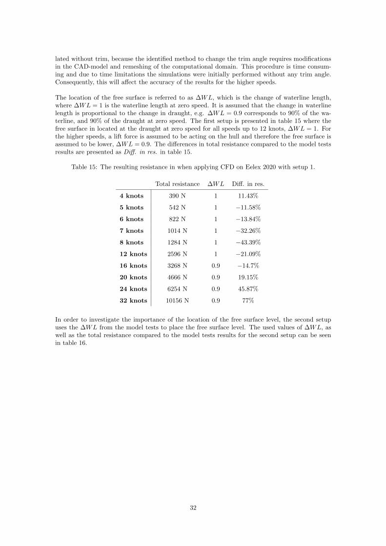
lated without trim, because the identified method to change the trim angle requires modificationsin the CAD-model and remeshing of the computational domain. This procedure is time consum-ing and due to time limitations the simulations were initially performed without any trim angle.Consequently, this will affect the accuracy of the results for the higher speeds.

The location of the free surface is referred to as ∆WL, which is the change of waterline length,where ∆WL = 1 is the waterline length at zero speed. It is assumed that the change in waterlinelength is proportional to the change in draught, e.g. ∆WL = 0.9 corresponds to 90% of the wa-terline, and 90% of the draught at zero speed. The first setup is presented in table 15 where thefree surface in located at the draught at zero speed for all speeds up to 12 knots, ∆WL = 1. Forthe higher speeds, a lift force is assumed to be acting on the hull and therefore the free surface isassumed to be lower, ∆WL = 0.9. The differences in total resistance compared to the model testsresults are presented as Diff. in res. in table 15.

Table 15: The resulting resistance in when applying CFD on Eelex 2020 with setup 1.

Total resistance ∆WL Diff. in res.

4 knots 390 N 1 11.43%

5 knots 542 N 1 −11.58%

6 knots 822 N 1 −13.84%

7 knots 1014 N 1 −32.26%

8 knots 1284 N 1 −43.39%

12 knots 2596 N 1 −21.09%

16 knots 3268 N 0.9 −14.7%

20 knots 4666 N 0.9 19.15%

24 knots 6254 N 0.9 45.87%

32 knots 10156 N 0.9 77%

In order to investigate the importance of the location of the free surface level, the second setupuses the ∆WL from the model tests to place the free surface level. The used values of ∆WL, aswell as the total resistance compared to the model tests results for the second setup can be seenin table 16.

32

Table 16: The resulting resistance in when applying CFD on Eelex 2020 with setup 2.

Total resistance ∆WL Diff. in res.

4 knots 390 N 1 11.43%

5 knots 542 N 1 −11.58%

6 knots 822 N 1 −13.84%

7 knots 1008 N 0.99 −32.67%

8 knots 1134 N 0.96 −49.21%

12 knots 1832 N 0.86 −44.32%

16 knots 2192 N 0.74 −42.78%

20 knots 3144 N 0.72 −19.71%

24 knots 4362 N 0.72 1.77%

32 knots 8046 N 0.76 40.84%

It can be seen in table 15 and 16 that the location of the free surface have a great impact on theresults, especially for the planing speeds, which was expected due to the impact of the runningattitude. For semi-planing speeds, a more accurate location of the free surface results in less accu-rate resistance predictions, which might be explained by the lack of trim angle. In order to get themost accurate resistance predictions, it has been decided to proceed with the results from setup 1for speeds up to 16 knots and the results from setup 2 for higher speeds.

The pressure resistance, viscous resistance and total resistance forces are presented in table 17

Table 17: The resulting resistance when applying CFD on Eelex 2020.

4 knots 5 knots 6 knots 7 knots 8 knots

Pressure resistance 320 N 436 N 690 N 840 N 1018 N

Viscous resistance 70 N 106 N 132 N 174 N 266 N

Total resistance 390 N 542 N 822 N 1014 N 1284 N

12 knots 16 knots 20 knots 24 knots 32 knots

Pressure resistance 1950 N 2222 N 1980 N 2680 N 4860 N

Viscous resistance 646 N 1044 N 1164 N 1682 N 3186 N

Total resistance 2596 N 3268 N 3144 N 4362 N 8046 N

According to the theory in section 2.1, the viscous resistance should be dominating in the displace-ment speeds. However, it can be seen in table 17 that the pressure resistance is larger than theviscous resistance for all speeds in the CFD simulations. Figure 20 shows the volume fraction onthe bottom of the hull, i.e. the distribution of the two phases air and water occupying the hullsurface for all different speeds. Water is displayed in red and air in blue.

33

(a) 4 knots. (b) 5 knots.

(c) 6 knots. (d) 7 knots.

(e) 8 knots. (f) 12 knots.

(g) 16 knots. (h) 20 knots.

(i) 24 knots. (j) 32 knots.

Figure 20: Volume fraction on the bottom of the hull for all speeds.34

6.5 Comparison

This section will present a comparison between the results from applied methods and the valuesfrom the conducted model tests. The model test results will serve as a reference value to determinethe accuracy of the other methods. For displacement, the speeds 4− 8 knots are regarded and themodel tests are compared with results from Holtrop & Mennen and CFD simulations, as well asthe Savitsky method for the higher speeds in the range. For planing, the speeds 12− 32 knots areregarded and model tests are compared with the Savitsky method and CFD simulation results.More detailed information about the results can be found in Appendix E.

6.5.1 Resistance predictions

The resulting resistance force from all the applied methods can be seen in figure 21. Since Holtrop &Mennen is a method for displacement hulls and Savitsky is a method for planing hulls, theoretically,the semi-empirical methods should leave a gap where the resistance can not be predicted. Thisgap refers to the Froude numbers which characterize a semi-planing hull, which neither of thesemi-empirical methods are valid for. However, since the Savitsky method is applicable from 7knots for Eelex 2020, the semi-planing speed range is covered by the semi-empirical methods.

Figure 21: The resulting resistance force from all the applied methods on Eelex 2020.

35

For displacement speeds, i.e. the speeds 4 − 8 knots the resulting resistance force for Eelex 2020can be seen in figure 22.

Figure 22: Resulting resistance force for Eelex 2020 in displacement speeds.

It can be seen in figure 22 that Holtrop & Mennen over-estimates the resistance, while CFD under-estimates the resistance for all speeds except for 4 knots. The difference in resistance force inpercentage between Holtrop & Mennen and model test and CFD and model tests, respectively,indicates how well the methods predicts resistance assuming that the model tests provide anaccurate prediction, see table 18. The difference in resistance force between the Savitsky methodand model tests for 7 and 8 knots can also be seen in the table.

Table 18: Deviation in resistance force for Holtrop & Mennen, CFD and the Savitsky method frommodel test results.

4 knots 5 knots 6 knots 7 knots 8 knots

Froude number 0.24 0.30 0.36 0.42 0.48

Holtrop & Mennen 2.2% 18.9% 70.6% 54.2% 30.5%

CFD 11.43% −11.58% −13.84% −32.6% −43.39%

Savitsky - - - 10.7% −19.6%

The greatest deviation for Holtrop & Mennen, 70.6%, is found Froude number Fn = 0.36. It isa much larger deviation than the errors found in previous studies, where a maximum of 16% wasfound, however for Fn < 0.2. For the same Froude number, Fn = 0.36, the deviation for CFD is−13.84% and significantly lower than the deviation for Holtrop & Mennen. The greatest deviationfor CFD is found for Fn = 0.48 and is −43.39%. For the lower speeds in the range, the devia-tions are close to the 10% that are found in previous studies. Although the error increases withthe speed, CFD seems to result in more accurate predictions in general. However, the Savitskymethod provides results with better accuracy than both Holtrop & Mennen and CFD for 7 and 8knots.

36

For planing speeds, i.e. 12− 32 knots, the resulting resistance force for Eelex 2020 can be seen infigure 23.

Figure 23: Resulting resistance force for Eelex 2020 in planing speeds.

In figure 23 it can be seen that CFD under-estimates the results for the lower speeds in therange, while it for the higher speeds over-estimates the resistance force. The Savitsky method isconsistently under-estimating the resistance and the curves for the Savitsky method and modeltests have similar shapes. The difference in resistance force in percentage between the Savitskymethod and model tests, and CFD and model tests respectively can be seen in table 19.

Table 19: Difference in resistance force in percentage between model tests and Savitsky.

12 knots 16 knots 20 knots 24 knots 32 knots

Froude number 0.72 0.96 1.20 1.44 1.92

Savitsky −20.8% −18.7% −13.7% −13.9% −18.8%

CFD −21.09% −14.7% −19.71% 1.77% 40.84%

For the Savitsky method, the largest deviation of −20.8% is found for Fn = 0.72. This is asignificant smaller deviation than the ones found for Holtrop & Mennen at displacement speeds.The CFD results are less consistent than the results from the Savitsky method, which has anaverage error of 17.18%.

37

The Savitsky method shows good agreement on the resulting trim angles for the model tests, seefigure 24, for the speeds 12 − 32 knots. The greatest deviation of −15.3% are found for 16 knotsand the smallest deviation of −4.8% for 12 knots.

Figure 24: The resulting trim angle from model tests and the Savitsky method.

It can also be noted that Savitsky seems to under-predict the trim for the speeds 12− 32 knots.

6.5.2 Power predictions and efficiency

The resulting resistance power for displacement and planing speeds can be seen in table 20 and 21respectively.

Table 20: Resulting resistance power from applying model tests, Holtrop & Mennen, CFD and theSavitsky method on Eelex 2020 in displacement speeds.

4 knots 5 knots 6 knots 7 knots 8 knots

Froude number 0.24 0.30 0.36 0.42 0.48

Model tests 0.7 kW 1.6 kW 2.9 kW 5.4 kW 9.3 kW

Holtrop & Mennen 0.74 kW 1.88 kW 5.03 kW 8.31 kW 12.18 kW

CFD 0.80 kW 1.39 kW 2.54 kW 3.65 kW 5.28 kW

Savitsky - - - 5.56 kW 7.5 kW

Table 21: Resulting resistance power from applying model tests, the Savitsky method, and CFDon Eelex 2020 in semi-planing and planing speeds.

12 knots 16 knots 20 knots 24 knots 32 knots

Froude number 0.72 0.96 1.20 1.44 1.92

Model tests 20.3 kW 31.5 kW 40.3 kW 52.9 kW 94.0 kW

Savitsky 16.1 kW 25.6 kW 34.8 kW 45.5 kW 76.4 kW

CFD 16.03 kW 26.90 kW 32.35 kW 53.86 kW 132.46 kW

38

Table 22 presents the different components of the total efficiency. The first four rows representthe input values required to calculate the propulsion efficiency ηD, where the open water propellerefficiency is an estimation for the single propeller used for Eelex 2020. The last three rows presentthe gear box efficiency, motor efficiency and battery capacity for Eelex 2020.

Table 22: Efficiency for Eelex 2020.

Symbol Value Unit

Number of propellers 1 -

Open water propeller efficiency ηO 60 %

Relative rotary efficiency ηR 100 %

Hull efficiency ηH 106 %

Propulsion efficiency ηD 63 %

Gear box efficiency ηG 96 %

Motor efficiency ηM 95 %

Battery capacity EB 120 kWh

The resulting range for Eelex 2020 from the different methods, assuming constant speed andincluding a sea margin of 15% to capture the influence of waves and wind, can be seen in figure25.

Figure 25: Resulting range for the different methods.

39

It can be seen in figure 25 that the range decreases significantly from approximately 300 − 50nautical miles (NM) for increasing speeds in the range of 4 − 12 knots, and both Holtrop &Mennen and CFD show this behaviour. After 12 knots, the curve flattens out, and the decreasein range is not as steep as for the lower speeds, according to all methods applied in the planingspeed range. The corresponding time for each range is presented in table 23 and 24.

Table 23: Resulting time and range for displacement speeds.

Model testHoltrop &Mennen

CFD Savitsky

Time Range Time Range Time Range Time Range

4 knots 86h 344 NM 81h 327 NM 75h 300 NM - -

5 knots 37h 188 NM 32h 160 NM 43h 216 NM - -

6 knots 20h 124 NM 12h 72 NM 23h 142 NM - -

7 knots 11h 78 NM 7h 50 NM 16h 115 NM 10 h 70 NM

8 knots 6h 51 NM 5h 39 NM 11h 91 NM 8 h 64 NM

Table 24: Resulting time and range for planing speeds.

Model test Savitsky CFD

Time Range Time Range Time Range

12 knots 3h 35 NM 3h 45 min 45 NM 3h 45min 45 NM

16 knots 1h 50min 30 NM 2h 20min 37 NM 2h 15min 35 NM

20 knots 1h 30min 29 NM 1h 45min 34 NM 1h 50min 37 NM

24 knots 1h 27 NM 1h 20min 31 NM 1h 26 NM

32 knots 40min 20 NM 45min 25 NM 30min 14 NM

It can be seen in table 24 that all of the three methods for resistance predictions in planing speeds,and especially in the cruising speed of 24 knots, give similar predictions of the range. However, forthe displacement speeds the results of the range predictions are more varying.

6.6 Evaluation

Table 25 presents the evaluation of the methods in a Pugh Matrix. Model tests are set as a base-line, and each method is rated from -2 to +2 on each criterion, where -2 means that the methodperforms worse than the baseline on that particular criterion, and +2 better than the baseline.

The weights are relative values, where the most important criterion is assigned the highest valueof the weighting scale, i.e. 5, and the least important criterion is assigned the lowest value, i.e. 1.Since the weights are not absolute values, the weighting must be re-evaluated if new criteria areadded and the ranking changes. A criterion with the weight 1, is therefore not irrelevant but ofless importance than criteria with a higher value.

40

Table 25: Pugh Matrix with X Shore’s criteria.

Criteria Weight Model testsHoltrop &Mennen

Savitsky CFD

Low

tim

eco

nsu

mp

tion Preparing calculations 4 0 +2 +2 +1

Performing calculations 3 0 +2 +2 -1

Interpreting results 5 0 +2 +2 +2

Low

cost

Equipment* 2 0 +2 +2 +1

Hig

hqu

ali

ty Accuracy 1 0 -2 -1 -1

Precision 3 0 -2 0 -1

Hig

hac

cess

ibil

ity

Equipment* 5 0 +2 +2 +1

Competence 4 0 +2 +2 0

Score 0 38 45 14

* Equipment refers to software licenses, hardware, tools and facilities.

The method with the highest total score of 45 is the Savitsky method. Holtrop & Mennen has aslightly lower score, 38, due to its low scores on the quality criteria. CFD has the lowest total score,14, since it is much more time consuming and has a lower accessibility than the semi-empiricalmethods. It can be seen in the Pugh Matrix, table 25, that low time consumption and cost, andhigh accessibility have higher priority than high accuracy, when choosing a method to predict resis-tance in the design phase. Accuracy is therefore assigned the weight 1, not because it is irrelevant,but because it has lower priority. However, precision which is the other quality criteria is weightedhigher since the consistency of the results determines if the method can be used at all.

A low time consumption is of high importance, due to the fast-paced design processes at thecompany. It can be seen in the matrix that it is more important that determining input values andinterpreting results are less time consuming than the importance of the time spent on perform-ing the calculations. This means that the most important aspect of low time consumption is theactive work hours spent on the task. If running a CFD-simulation takes hours, or days, withoutdemanding active work hours and deliver results within time plan, it can still be a suitable method.The cost of equipment is ranked lower than both time consumption and accessibility. While costis an important aspect, equipment cost is assumed to be spread out over a long period of time.It might therefore be less expensive to invest in equipment to enable in-house approaches thanto constantly hire external consultants. Cost will consequently have less importance and not bea deciding factor. The accessibility of the equipment is however of bigger importance in order toenable in-house approaches. The same goes for competence, since competence deficiencies in thecompany require external consultants. Note that the weighting is set based on the purpose of thisstudy, i.e. to find a suitable approach to predict resistance for X Shore as a start-up company.

41

7. Discussion and ConclusionAll resistance predictions are made on a bare hull and in calm water conditions. When convertingthe resistance to range, a sea margin has been included in order to increase the accuracy of therange estimations. However, the estimated ranges for different speeds are, despite the sea mar-gin, higher than the ranges that can be expected from a real life scenario, where resistance fromappendages are present. Adding resistance from appendages will give more accurate results, butrequires modifications of the methods investigated in this study. Several aspects considering theefficiency might influence the outcomes of the methods, e.g. the hull efficiency which is calcu-lated using simplified equations and the open water propeller efficiency which is assumed to beconstant over the entire speed range. Moreover, energy losses from the batteries to the motor arenot accounted for. Since the study is limited to one hull, no conclusions can be drawn about theperformance of the methods in general.

The quality of the outcome of the Pugh Matrix depends on the selection of criteria. In orderfor the Pugh Matrix to guide the decision making process, all relevant criteria must be included,and no irrelevant criteria should be present in the matrix. The criteria in this study was selectedafter discussions between the authors and X Shore, and are assumed to be sufficient for the pur-pose of this study. However, to use this evaluation method in the future, X Shore needs to ensurethat all relevant aspects are covered in the selected criteria. The company might prioritize thecriteria differently in future design processes, and the recommendations in this report might notbe suitable. However, the same evaluation process may still be useful in order to choose the mostsuitable method. Finally, it should be clarified that even though the selected criteria are relevantand the weighting corresponds to the company’s priorities, the method with the highest score isnot necessarily the most suitable in all cases. While a Pugh Matrix serves as a tool in the decisionmaking, decisions should not be based solely on the matrix scores.

The methods evaluated in this study is supposed to fill a gap in the early design phase. It isof importance that the methods have a sufficient precision to serve as a guide when making designchanges. The methods should give predictions of the right magnitude, as well as capture differ-ences between different designs, but the exact value of the resistance is not important in the earlydesign phase. In later design phases, when the design is set and more accurate predictions may bevaluable, the recommendations in this study may not be suitable.

The results from Holtrop & Mennen on Eelex 2020 deviate between 2.2% and 70.6% from themodel test results, which is a significantly larger error than 16% shown in a previous study. It canalso be concluded that the method has a low precision, and the predictions do not follow a clearpattern. The method is previously shown to be less accurate in cases where the hull geometry isclose to the applicability limits, and the fact that the length-beam ratio of Eelex 2020 is belowthe applicability limit is a possible explanation to the large deviations and low precision. BecauseHoltrop & Mennen is developed from model tests performed on a number of hulls, the method isonly applicable for hull geometries similar to the ones the equations are based on. This is clearlya disadvantage of the method, since it only can be applied when designing hulls with traditionalshapes and dimensions. To summarize, Holtrop & Mennen does not provide accurate resistancepredictions for Eelex 2020. Despite the low accuracy and precision, Holtrop & Mennen is a quickand user friendly method that does not require neither high competence nor advanced equipment.

The results from Holtrop & Mennen show that the wave resistance is the dominant resistancecomponent as the speed increases. This corresponds well with the theory presented in section 2.1,which states that the pressure resistance, i.e. the wave resistance, increases with increasing speed.This indicates that although Holtrop & Mennen over-estimates the resistance in an inconsistentway, the method seems to capture the theoretical behaviour of the resistance forces. It may there-fore be able to apply the method to compare different hull designs, because even though the valueof the resistance predictions are inaccurate, it may accurately indicate differences between hulldesigns. This is however just a speculation, and needs to be confirmed by further investigations.

42

For low speeds, corresponding to Fn ≤ 0.36, the CFD results deviate maximum 13.84% from themodel test results. The deviations are within acceptable limits, but slightly higher than the 10%error found in previous studies. For 7 and 8 knots, the error is larger, 32.6% and 43.39% respec-tively. Compared to Holtrop & Mennen, the CFD results are more consistent, especially for thelower speeds in the displacement range. CFD resulted in a total score of 14 in the Pugh Matrix,which is less than half of the total score for Holtrop & Mennen. The drawback with CFD is thetime consumption, which is significantly higher than the time for Holtrop & Mennen. However,the time required to perform a CFD simulation covering all speeds simulated in this study takesapproximately one week in total time, and three days in active time, excluding the mesh conver-gence study. The time consumption is considered acceptable and although it is higher than the 30minutes Holtrop & Mennen takes, one week can be reasonable to spend on resistance predictions.Another aspect influencing the Pugh Matrix outcome is the highly prioritized accessibility, whereCFD requires both high competence and suitable hardware and licence, which Holtrop & Mennendoes not. If CFD will be applied in-house, X Shore would need to invest in suitable equipment andcompetence, which might not be an obstacle due to that low cost is not highly prioritized. OnceX Shore have equipment and competence, the accessibility will increase. Based on the argumentsmentioned above, in combination with the very low precision and accuracy from Holtrop & Men-nen, CFD is a more suitable method for X Shore than Holtrop & Mennen, despite the contradictoryPugh Matrix scores. However, the Savitsky method applied for 7 and 8 knots predicts results withbetter accuracy than both Holtrop & Mennen and CFD.

Compared with the model test results, the Savitsky method under-predicts the results by 20.8%−13.7%, with an average deviation of 17.18% for the speeds 12 − 32 knots. The maximum erroris for Fn = 0.72, which means that although the applicability criteria are fulfilled, the boat hasnot reached planing and a large error can therefore be expected. It can be seen in figure 23, thatalthough the Savitsky method under-predicts the resistance for the speed range 12− 32 knots, theshape of the curve is similar to the curve for model tests. For 7 knots, the Savitsky method over-predicts the resistance with 10.7%, which deviates from the behaviour of the method for the higherspeeds. Nevertheless, the Savitsky method provides the most precise results of all applied methodsfor the speeds that fulfills the applicability criteria of the Savitsky method. The average deviationof the absolute values for the Savitsky method applied to the speeds 7 − 32 knots is 17.58%. Bymodifying the method and include a correction factor of 1.1758 the accuracy can be improved, seeAppendix F. This correction factor has been added in the developed Python program.

The predicted trim angles from the Savitsky method correspond well with the angles obtainedin the model tests, and the error is between 4.8% and 15.3%. The maximum deviation is 0.77◦ andoccurs at Fn = 0.96. Like Holtrop & Mennen, the Savitsky method is a semi-empirical methodbased on experiments, and its applicability is limited to hull shapes similar to the ones that theequations are derived from. However, Eelex 2020 fulfills the applicability criteria, which indicatesthat the method should give acceptable results. Holtrop & Mennen and the Savitsky method havein common that the input values are easily changed, which enables quick adjustments of the hullcharacteristics and indications of their impact on the resistance. According to section 2.1, LCGshould be positioned at 40%−45% of the chine length from the transom for displacement hulls, and25%− 35% of the chine length for planing hulls. At Eelex 2020, LCG is positioned approximately40% forward of the transom, which is a good position for displacement, but not optimal for planingspeeds. With the flexibility that the Savitsky method offers, LCG can easily be adjusted in orderto determine how sensitive the total resistance is to the position. To make a similar study withCFD would take significantly more time and effort.

The CFD simulations for planing speeds vary more than the results from the Savitsky method.While the smallest error is very close to the model test result, only 1.77% deviation at Fn = 1.44,the largest error is as much as 40.84% at Fn = 1.92. Previous studies show that CFD shouldyield results with less than 10% error, and that they generally are smaller than the errors from theSavitsky method. The results from this study show the opposite, and one possible explanation isthat the ITTC guidelines used are developed for Froude numbers of the order 0.1 and rarely above1. Thus, above 16 knots, Fn > 1 for Eelex 2020, the ITTC guidelines may not be appropriate.

43

Furthermore, the fact that trim angle is neglected and the running attitude is not accounted forproperly, affects the accuracy negatively. According to the Pugh Matrix, the Savitsky methodis the most suitable method for resistance predictions in planing speeds, with a total score of 45compared to 14 for CFD. Due to that CFD both shows lower precision, and requires more timeto perform, the recommendation is to apply the Savitsky method for resistance predictions in theplaning speed range.

For semi-planing, i.e. 0.4 < Fn < 1 and speeds 7 − 16 knots, the running attitude of the hullvaries significantly compared to displacement speeds, and consequently the resistance is harder topredict. Since the trim angle has been neglected from the simulations, this might be the explana-tion to the large deviations of the CFD results, especially for 7 and 8 knots. Possibly, a dynamicmesh which captures the hull motions, and therefore identifies the running attitude, can improvethe CFD results in this speed range.

In contrast to the semi-empirical methods, the applicability of CFD is not limited by hull ge-ometry. The limitations for CFD are rather competence and computer capacity. The differencesbetween the results from setup 1 and setup 2 show that the resistance predictions are sensitive tothe location of the free surface. Estimating the free surface level accurately requires knowledge ofthe behaviour of planing hulls, alternatively data from model tests or other methods. For planingspeeds, the largest deviation is 40.84% for 32 knots when the free surface location is changed ac-cording to model test data. It should be noted that ∆WL is larger for 32 knots than for 20 and 24knots which could be a source of error. Adjusting the free surface to the same level as for 20 and24 knots would decrease the error, but the result would probably still be over-estimated. Qualifiedestimations of the free surface has been proven to be of importance. Another interesting aspectis the effect of a potential implemented trim in the simulations. All the performed simulations inthis study are done without any trim, but a trim angle would probably improve the results since itwould increase how accurate the running attitude is modelled. Estimating the trim would in thesame way as the free surface estimations require a qualified guess, and since the Savitsky methodhas shown good agreement of the trim angles, a suggestion is to combine CFD and the results oftrim angle from the Savitsky method. Combining CFD and the Savitsky method has been testedfor 12 and 32 knots, see Appendix F. None of the simulations did converge, and it can be concludedthat in order to implement trim in the CFD simulations, at least a new mesh convergence studyneeds to be conducted.

The selection of methods and models for the CFD simulations is based on theory in chapter4. However, other methods and models are available and no further investigation regarding theimpact of them has been performed. In this study, a mesh convergence study was performed forone Froude number. Consequently, the dimensionless wall distance y+ is the same in all simula-tions, which is an inaccurate assumption. To increase the accuracy of the simulations and ensurethe quality of the mesh, mesh convergence studies should be made over the whole range of Froudenumbers and the value of the dimensionless wall distance should be verified. The blue areas on thehull in figure 20 symbolize air, which may indicate that numerical ventilation occurs. This woulddecrease the total resistance prediction, but looking at figure 20i for 24 knots, a large area of airin the middle of the hull can be seen. However, the result for 24 knots has the smallest deviationof all simulated speeds, which may indicate that the blue areas have another explanation thannumerical ventilation. By checking and adjusting the dimensionless wall distance, the effects fromthe potential numerical ventilation can be reduced and the overall quality can be improved. Sincethe y+ value is supposed to capture the flow close to the hull surface, poor meshing of the boundarylayer will affect the total resistance. The fact that the y+ value has not been checked in this studymight explain why the viscous resistance is lower than the pressure resistance, even for low speeds.Another way of increasing the accuracy and quality of the simulation is to change the convergencecriteria, i.e. lower the residuals. However, the simulations have shown good convergence and stablesolutions with the residuals used in this study, and the quality is assumed to be sufficient in orderto determine the suitability of CFD as a method for X Shore.

44

Besides the possibility to easily evaluate different hulls by simply changing the CAD-file, CFDhas a number of advantages. Although the purpose of applying CFD in this study was to predictresistance, the simulations can also predict e.g. pressure distribution on the hull, wave pattern,and turbulence. For that reason, it might be useful in the later design phases and even for higherspeeds, if a more complex setup is applied. Additionally, CFD has a lower economical cost thanmodel tests. The major advantage of model tests is that it provides accurate results. Even thoughit is both costly and time consuming, there are several reasons why it may be useful to performoccasionally, e.g. when predictions with high accuracy are needed. Additionally, model tests canbe used to verify and adjust other methods. However, it is not necessary to include model tests inevery design process, and if used, it should not be applied in early design phases. As X Shore has aquick manufacturing process and access to the full-scale hulls, another way to validate and adjustthe methods is to perform full-scale tests where total resistance and trim angle are measured.

7.1 Conclusion

From the results, it can be concluded that the recommended approach for X Shore to implementin their design process to predict resistance is the Savitsky method for all speeds that fulfils theapplicability criteria of the method. If predictions for lower speeds are of interest, CFD is therecommended method. When applying the Savitsky method, it is recommended to follow theprocedure in section 6.3 and use the program developed by the authors, where the correctionfactor has been included. The CFD simulations should be applied according to section 6.4.

45

8. Future workOne focus for future work should be the mesh used in the CFD simulations. The mesh convergencestudy have only been conducted for one Froude number, and to improve the accuracy mesh conver-gence should be checked for all Froude numbers corresponding to speeds between 4 and 32 knots.A suggestion is to perform the CFD simulations with a fixed trim on the hull, in order to determinethe sensitivity of the results to changes of the trim angle. It would also be of interest to comparethe results from this study with results obtained from simulations performed with a dynamic mesh.

Another improvement that would result in more accurate estimations of the range would be toinclude appendages in the methods. This requires a re-evaluation of the recommended systematicapproach, since it may influence the accuracy of the different methods. To add resistance fromappendages in Holtrop & Mennen is straightforward, since the method include it by default. How-ever, for the Savitsky method and CFD, it is more complicated. The Savitsky method does nothandle appendages by default and need to be modified. In order to capture the influence fromappendages in CFD simulations, appendages need to be properly meshed. Furthermore, the CFDmethods and schemes would need to be re-evaluated to be suitable for simulations with appendages.

Even though the semi-empirical methods, and especially Holtrop & Mennen, deviate significantlyfrom model test results, it could be of interest to apply the methods on different hulls and inves-tigate whether it can be used for comparisons of hulls.

46

References[1] Statistiska centralbyran, Utslapp av vaxthusgaser fran inrikes transporter efter vaxthusgas och

transportslag. ar 1990 - 2018, 2019. [Online] Available at http://www.statistikdatabasen.scb.se/pxweb/sv/ssd/START__MI__MI0107/MI0107InTransp/table/tableViewLayout1/

(Accessed 2020-02-19).

[2] Regeringskansliet, Sverige ska bli ett fossilfritt valfardsland, 2018. [Online] Available at https:/ / www . regeringen . se / artiklar / 2018 / 04 / sverige - ska - bli - ett - fossilfritt -

valfardsland/ (Accessed 2020-02-19).

[3] P-O. Moksnes, L. Eriander, J. Hansen, J. Albertsson, M. Andersson, U. Bergstrom, J. Carl-strom, J. Egardt, R. Fredriksson, L. Granhag, F. Lindgren, K. Nordberg, I. Wendt, S.Wikstrom, E. Ytreberg, “Fritidsbatars paverkan pa grunda kustekosystem i Sverige”, Havs-miljoinstitutets Rapport 2019:3, 2019.

[4] E. C. Tupper, Introduction to naval architecture. Butterworth-Heinemann, 2013, isbn: 978-0-08-098237-3.

[5] A. F. Molland, The Maritime engineering reference book. Butterworth-Heinemann, 2008,isbn: 978-0-7506-8987-8.

[6] X Shore, About X Shore, 2020. [Online] Available at https://www.xshore.com/about-x-

shore (Accessed 2020-03-09).

[7] P. Voxakis, “Ship hull resistance calculations using cfd methods”, Massachusetts Institute ofTechnology, 2012.

[8] Z. Zhang, H. Liu, S. Zhu, F. Zhao, “Application of cfd in ship engineering design practiceand ship hydrodynamics”, Journal of Hydrodynamics, Ser. B, vol. 18, no. 3, pp. 315–322,2006.

[9] K. Garme, “Ship resistance and powering”, KTH Center of Naval Architecture, 2012.

[10] D. Frisk and L. Tegehall, “Prediction of high-speed planing hull resistance and runningattitude”, CHALMERS UNIVERSITY OF TECHNOLOGY, 2015.

[11] J. M. Almeter, “Resistance prediction of planing hulls: State of the art”, Marine Technology,vol. 30, no. 4, pp. 297–307, 1993.

[12] O. M. Faltinsen, Hydrodynamics of High-Speed Marine Vehicles. New York: Cambridge Uni-versity Press, 2005, isbn: 978-0-521-84568-7.

[13] A. Kukner and A. Yasa, “High speed planing hulls resistance prediction methods and com-parison”, Istanbul Technical University, Turkey, 2011.

[14] L. Larsson and R. Eliasson, Principles of Yacht Design. International Marine/Ragged Moun-tain Press; 2 edition, 2000, pp. 183–196, isbn: 978-0071353939.

[15] L. Birk, Fundamentals of ship hydrodynamics. John Wiley & Sons, 2019, isbn: 978-1-1188-5551-5.

[16] Brusa, “HSM1 - Hybrid Synchronous Motor”.

[17] L. Nikolopoulos, E. Boulougouris, “A study on the statistical calibration of the holtropand mennen approximate power prediction method for full hull form, low froude numbervessels”, Journal of Ship Production and Design, vol. 35, no. 1, pp. 41–68, 2018. doi: https://doi.org/10.5957/JSPD.170034.

[18] International Towing Tank Conference, “Practical guidelines for ship resistance CFD”, ITTC– Recommended Procedures and Guidelines, vol. 7.5–03–02–04, 2014.

[19] J. Holtrop, G.G.J. Mennen, “An approximate power prediction method”, International Ship-building Progress, vol. 29, no. 335, pp. 166–170, 1982.

[20] D. Savitsky, “Hydrodynamic design of planing hulls”, The Society of Naval Architects andMarine Engineers, vol. 1, no. 04, 1964.

47

[21] J. Carlton, Marine propellers and propulsion. Butterworth-Heinemann, 2007, isbn: 978-0-7506-8150-6.

[22] International Towing Tank Conference, “Testing and extrapolation methods, general guide-lines for uncertainty analysis in resistance towing tank tests”, ITTC – Recommended Proce-dures and Guidelines, vol. 7.5–02–02–02, 2008.

[23] International Towing Tank Conference, “Practical guidelines for ship CFD applications”,ITTC – Recommended Procedures and Guidelines, vol. 7.5–03–02–03, 2014.

[24] International Towing Tank Conference, “Resistance test”, ITTC – Recommended Proceduresand Guidelines, vol. 7.5–02–02–01, 2011.

[25] F. Cakıcı, O.F Sukas, O. Usta, A.D.Alkan, “A computational investigation of a planing hullin calm water by u-ranse approach”, International conference on advances in applied andcomputational mechanics, 2015.

[26] International Towing Tank Conference, “Practical guidelines for ship CFD applications”,ITTC – Recommended Procedures and Guidelines, vol. 7.5–03–02–03, 2011.

[27] ANSYS Inc., “ANSYS Fluent 12.0 Theory Guide”, 2009.

[28] A. Persson, SSPA, [Pesonal communication by e-mail] (2020-02-21).

[29] H. K. Versteeg and W. Malalasekera, An Introduction to Computation Fluid Dynamics: TheFinite Volume Method. Pearson Education Limited, 2007, isbn: 9780131274983.

[30] R. A. Bengt Andersson and L. Hakansson, Computational Fluid Dynamics for Engineers.Cambridge University Press, 2012, isbn: 9781139205795.

[31] F. Stern, J. Yang, Z. Wang, H. Sadat-Hosseini, M. Mousaviraad, S. Bhushan, T. Xing,“Computational ship hydrodynamics: Nowadays and way forward”, International Shipbuild-ing Progress, vol. 60, no. 1-4, pp. 3–105, 2013. doi: 10.3233/ISP-130090.

[32] A. Gray-Stephens, T. Tezdogan, S. Day, “Strategies to minimise numerical ventilation in CFDsimulations of high-speed planing hulls”, Proceedings of the ASME 2019 38th InternationalConference on Ocean, Offshore and Arctic Engineering, 2019.

[33] I. M. Viola, R. G. J. Flay, R. Ponzini, “Cfd analysis of the hydrodynamic performance of twocandidate america’s cup ac33 hulls”, Transactions of the Royal Institution of Naval ArchitectsPart B: International Journal of Small Craft Technology, vol. 154, no. 1, B1–B12, 2012. doi:https://doi.org/10.3940/rina.ijsct.2012.b1.113.

[34] A. Rosen, “Introduction to seakeeping”, KTH Center of Naval Architecture, 2011.

[35] ANSYS Inc., “ANSYS Fluent Tutorial Guide”, 2017.

[36] ANSYS Inc., “ANSYS Fluent User’s Guide”, 2013.

[37] NASA, Evaluating Iterative Convergence, 2008. [Online] Available at https://www.grc.

nasa.gov/WWW/wind/valid/tutorial/iterconv.html (Accessed 2020-02-10).

[38] H. Kerzner, Project management: a systems approach to planning, scheduling, and controlling.John Wiley & Sons, 2017, isbn: 978-1-1191-6537-8.

[39] D. for Communities and L. Government, “Multi-criteria analysis: A manual”, Departmentfor Communities and Local Government: London, 2009.

[40] D. S. Burge, “The systems engineering tool box”, 2009.

[41] F. S. Stefano Brizzolara, “Accuracy of cfd codes in the prediction of planing surface hydrody-namic characteristics”, University of Genoa, Department of Naval Architecture and MarineTechnology, Italy, 2007.

[42] J. Zelle, Graphics.py, [Online] Available at https://mcsp.wartburg.edu/zelle/python/

graphics.py (Accessed 2020-04-06).

[43] J. Holtrop, “A statistical re-analysis of resistance and propulsion data”, International Ship-building Progress, vol. 31, no. 363, pp. 3–5, 1984.

48

A. Holtrop & Mennen

Nomenclature

ABT = transverse bulb area at the positionwhere the still-water surface intersects the stemAM = midships cross-sectional areaAT = immersed part of the transverse area ofthe transom at zero speedAWP = waterplane areaB = maximum breadthCA = correlation allowance coefficientCB = block coefficientCf = friction coefficientCM = midship section coefficientCP = prismatic coefficientCWP = waterplane area coefficientD = average draughtDAP = draught at aft perpendicularDFP = draught at forward perpendicularFn = Froude numberFni = Froude number based on the immersionFnT = Froude number based on the transom im-mersiong = gravitational accelerationhB = position of the center of the transversearea ABT above the keel linelcb = longitudinal position of the center of buoy-ancy forward of 0.5L as percentage of LLWL = length on waterlineLR = length of the runLPP = length between perpendicularsPB = coefficient as a measure for the emergence

of the bowRA = model-ship resistanceRAPP = resistance of appendagesRB = additional pressure resistance of bulbousbow near the water surfaceRe = Reynolds numberRF = frictional resistance according to ITTCformulationRtotal = total resistance of a shipRTR = additional pressure resistance of im-mersed transom sternRW = wave-making and wave-breaking resis-tanceRW−A = wave-making and wave-breaking resis-tance for Fn < 0.4RW−B = wave-making and wave-breaking resis-tance for Fn > 0.55RW−C = wave-making and wave-breaking resis-tance for 0.4 < Fn < 0.55S = wetted surface of the hullSAPP = wetted surface of the appendagesU = ship velocity(1 + k1) = form factor describing the viscous re-sistance of the hull form in relation to RF(1 + k2) = appendage resistance factor∇ = volume displacementν = kinematic viscosityρ = density of the fluid

If nothing else is specified, the equations in this appendix come from Holtrop & Mennen [19].

The total resistance is subdivided into

Rtotal = RF (1 + k1) +RAPP +RW +RB +RTR +RA (A.1)

and is determined by the following steps.

Step 1:The first term, RF is the frictional resistance according to the ITTC formulation [18]

RF =1

2ρU2CfS (A.2)

where ρ is the density of the water, U is the speed of the boat and S is the wetted surface of thehull. Cf is the friction coefficient [23] defined as

Cf =0.075

[log10(Re)− 2]2(A.3)

I

where Re is the Reynolds number defined as

Re =ULPPν

(A.4)

where LPP is the length between perpendiculars and ν is the kinematic viscosity [22].

The wetted surface of the hull can be approximated as

S =LWL(2D +B)√

(CM )(0.453 + 0.4425CB − 0.2862CM

− 0.003467

(B

D

)+ 0.3696CWP ) + 2.38

(ABTCB

)(A.5)

where LWL is the waterline length, B is the maximum breadth and ABT is the transverse sectionalarea of the bulb at the position where the still-water intersects the stem. The average draught Dis defined as

D =DFP +DAP

2(A.6)

where DFP is the draught at the forward perpendicular and DAP is the draught at the aft per-pendicular of the hull. CM is the midship section coefficient, CB is the block coefficient and CWP

is the waterplane area coefficient defined as

CM =AMBD

(A.7)

CB =∇

LPPBD(A.8)

CWP =AWP

LB(A.9)

where AM is the immersed midship sectional area at LWL/2, ∇ is the displacement volume andAWP is the waterplane area [9].

Step 2:The frictional resistance is multiplied with a form factor (1 + k1) describing the viscous resistanceof the hull form in relation to RF . The form factor is defined as

(1 + k1) = c13(0.93 + c12

(B

LR

)0.92497

(0.95− CP )−0.521448(1− CP + 0.0225lcb)0.6906) (A.10)

where lcb is the longitudinal position of the center of buoyancy forward of 0.5LWL as a percentageof LWL. The prismatic coefficient CP is based on LPP and defined as [9]

CP =∇

LPPAM(A.11)

In the form factor formula, LR is a parameter reflecting the length of the run and is defined as

LR = LWL

(1− CP + 0.06CP lcb

4CP − 1

)(A.12)

The form factor does also contain two coefficients, c12 and c13. The first one is defined as

II

c12 =

(D

LWL

)0.2228446

when(

DLWL

)> 0.05

48.20(

DLWL

− 0.02)2.078

+ 0.479948 when 0.02 <(

DLWL

)< 0.05

0.479948 when(

DLWL

)< 0.02

(A.13)

The other coefficient c13 is defined as

c13 = 1 + 0.003Cstern (A.14)

and accounts for the specific shape of the afterbody related to the coefficient Cstern which havethe tentative guidelines presented in table A.1.

Table A.1: Tentative guidelines for the specific shape of the afterbody of the ship.

Afterbody form Cstern

V-shaped sections -10

Normal section shape 0

U-shaped sections with Hogner stern +10

Step 3:The appendage resistance is the next term in the total resistance formulation and it is defined as

RAPP = 0.5ρU2SAPP (1 + k2)eqCf (A.15)

where SAPP is the wetted surface of the appendages and (1 + k2) is the appendage resistancefactor. Tentative values for the factor (1 +k2) are presented in table A.2, obtained from resistancetests with bare and appended ship models.

Table A.2: Tentative values for the appendage resistance factor (1 + k2).

Approximate (1 + k2) values

Rudder behind skeg 1.5 - 2.0

Rudder behind stern 1.3 - 1.5

Twin-screw balance rudders 2.8

Shaft brackets 3.0

Skeg 1.5 - 2.0

Strut bossings 3.0

Hull bossings 2.0

Shafts 2.0 - 4.0

Stabilizer fins 2.8

Dome 2.7

Bilge keels 1.4

III

A combination of appendages is determined as

(1 + k2)eq =

∑(1 + k2)SAPP∑

SAPP(A.16)

Step 4:Following, the wave resistance RW is depending on the Froude number Fn, based on the waterlinelength LWL and defined as

Fn =U√gLWL

(A.17)

For the speed range Fn < 0.4, the wave resistance is defined as

RW−A = c1c2c5∇ρge(m1Fdn+m4cos(λF

−2n )) (A.18)

and for the speed range Fn > 0.55 the wave resistance is defined as

RW−B = c17c2c5∇ρge(m3Fdn+m4cos(λF

−2n )) (A.19)

where c1, c2, c5, c17, m1, m3, m4 and λ are coefficients, g is the gravitational acceleration andd = −0.9. [43] [19] For the speed range 0.4 < Fn < 0.55 the wave resistance is defined as

RW−C = RW−A0.4 +(10Fn − 4)(RW−B0.55

−RW−A0.4)

1.5(A.20)

which is an interpolation formula where RW−A0.4 is the wave resistance for Fn = 0.4 and RW−B0.55

is the wave resistance for Fn = 0.55 according to equation A.18 and A.19 respectively [43].

The first coefficient c1 is determined as

c1 = 2223105c3.786137

(D

B

)1.07961

(90− iE)−1.37565 (A.21)

and

c7 =

0.229577(

BLWL

)0.33333

when(

BLWL

)< 0.11

BLWL

when 0.11 <(

BLWL

)< 0.25

0.5− 0.0625(LWL

B

)when

(B

LWL

)> 0.25

(A.22)

The angle of the waterline at the bow in degrees with reference to the center plane is called thehalf angle of entrance, iE , neglecting the local shape at the stem. If this angle is unknown, it canbe determined as

iE = 1 + 89e

(−( L

B )0.80856

(1−CWP )0.30484(1−CP−0.0225lcb)0.6367(

LRB

)0.34574(

100∇L3WL

)0.16302)(A.23)

The second coefficient c2 accounts for the reduction of the wave resistance due to the action of abulbous bow and is defined as

c2 = e(−1.89√c3) (A.24)

IV

where the coefficient determining the influence of the bulbous bow on the wave resistance is definedas

c3 =0.56A1.5

BT

BD(0.31√ABT +DFP − hB)

(A.25)

where hB is the position of the center of the transverse area ABT above the keel line. Nextcoefficient express the influence of a transom stern on the wave resistance and is defined as

c5 =1− 0.8ATBDCM

(A.26)

where AT is the immersed part of the transverse area of the transom at zero speed. Following, c17

is defined as [43]

c17 = 6919.3C−1.3346M

(∇

L3WL

)2.00977(LWL

B− 2

)1.40692

(A.27)

The remaining coefficients m1, m3, m4 and λ are determined as follows [43] [19]

m1 = 0.0140407

(LWL

D

)− 1.75254

(∇1/3

LWL

)− 4.79323

(B

LWL

)− c16 (A.28)

where

c16 =

8.07981CP − 13.8673C2

P + 6.984388C3P when CP < 0.80

1.73014− 0.7067CP when CP > 0.80

(A.29)

m3 = −7.2035

(B

LWL

)0.326869(D

B

)0.605375

(A.30)

m4 = c150.4e(−0.034F−3.29n ) (A.31)

where

c15 =

−1.69385 whenL3

WL

∇ < 512

−1.69385 +LWL

∇1/3−8.0

2.36 when 512 <L3

WL

∇ < 1727

0.0 whenL3

WL

∇ > 1727

(A.32)

and

λ =

1.446CP − 0.03

(LWL

B

)when LWL

B < 12

1.446CP − 0.36 when LWL

B > 12

(A.33)

Step 5:The additional resistance RB due to the presence of a bulbous bow near the surface is defined as

RB =0.11e(−3P−2

B )F 3niA

1.5BT ρg

1 + F 2ni

(A.34)

where PB is the coefficient of the measure for the emergence of the bow defined as

V

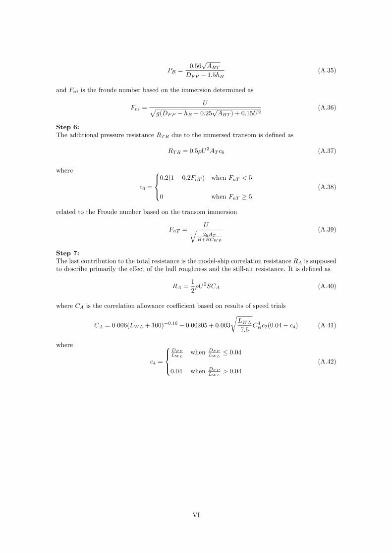
PB =0.56√ABT

DFP − 1.5hB(A.35)

and Fni is the froude number based on the immersion determined as

Fni =U√

g(DFP − hB − 0.25√ABT ) + 0.15U2

(A.36)

Step 6:The additional pressure resistance RTR due to the immersed transom is defined as

RTR = 0.5ρU2AT c6 (A.37)

where

c6 =

0.2(1− 0.2FnT ) when FnT < 5

0 when FnT ≥ 5

(A.38)

related to the Froude number based on the transom immersion

FnT =U√2gAT

B+BCWP

(A.39)

Step 7:The last contribution to the total resistance is the model-ship correlation resistance RA is supposedto describe primarily the effect of the hull roughness and the still-air resistance. It is defined as

RA =1

2ρU2SCA (A.40)

where CA is the correlation allowance coefficient based on results of speed trials

CA = 0.006(LWL + 100)−0.16 − 0.00205 + 0.003

√LWL

7.5C4Bc2(0.04− c4) (A.41)

where

c4 =

DFP

LWLwhen DFP

LWL≤ 0.04

0.04 when DFP

LWL> 0.04

(A.42)

VI

B. Savitsky method

Nomenclature

a = distance between the viscous drag compo-nent Df and the center of gravity, measurednormal to Df

B = beam of the boatc = the distance between the center of pressureand the center of gravity, measured parallel tothe keelCf = friction coefficientCL0 = lift coefficientCLβ = planing coefficientCp = center of pressureCV = planing coefficientD = total dragDf = viscous drag componentf = distance between the propeller axis and thecenter of gravity, measured normal to the pro-peller axisg = gravitational acceleration

LCG = longitudinal center of gravity measuredalong the keel from the transomRe = Reynolds numberU = ship velocityU1 = speed at the hull bottomV CG = vertical center of gravity measured fromthe keel lineβ = deadrise angleγ = specific weight of water∆ = displacement mass of the boatε = the inclination of the propeller axis relativeto the keelΛ = mean wetted length-beam ratioν = kinematic viscosityρ = density of waterτ = trim angleϕ = γ/g

If nothing else is specified, the equations in this appendix come from Savitsky [20].

Note that all input values must be expressed in imperial units, and not SI-units.

Step 1:Calculate the planing coefficients CV and CLβ :

CV =U√(gB)

(B.1)

CLβ =∆

12ϕU

2B2(B.2)

where g is the gravitational acceleration, B is the beam of the boat, ∆ is the displacement, U isthe speed of the boat and ϕ is defined as

ϕ =γ

g(B.3)

where γ is the specific weight of water.

Step 2:Making the following steps for a number of different values of τ will enable solving a momentequation and through linear interpolation finding the equilibrium trim angle.

Solve for CL0:

CLβ = CL0 − 0.0065βC0.60L0 (B.4)

VII

where β is the deadrise angle. The mean wetted length-beam ratio Λ is determined by solvingfollowing equation for Λ:

CL0 = τ1.1

(0.0120Λ1/2 + 0.0055Λ5/2

CV2

)(B.5)

The speed at the hull bottom U1 differs from the speed of the boat U and is approximated to

U1 = 0.95U (B.6)

Reynold’s number is calculated by

Re =U1ΛB

ν(B.7)

where ν is the kinematic viscosity of water. The frictional coefficient is calculated according toITTC [23] and defined as

Cf =0.0075

[log10(Re)− 2]2(B.8)

The viscous component of drag Df is defined as

Df =ϕU1

2ΛB2(Cf + ∆Cf )

2cos(β)(B.9)

where ∆Cf = 0.0004 according to ATTC standard. The total drag D can then be calculated by

D = ∆tan(τ) +ϕU1

2ΛB2(Cf + ∆Cf )

2cos(β)cosτ(B.10)

The center of pressure Cp can be calculated as

Cp = 0.75− 15.21C2

V

Λ2 + 2.39(B.11)

and is needed to determine the distance between the center of pressure and the center of gravity,measured parallel to the keel:

c = LCG− CpΛB (B.12)

where LCG is the longitudinal center of gravity measured along the keel from the transom. Thedistance between the viscous component of drag Df and the center of gravity, measured normalto Df is defined as

a = V CG− b

4tanβ (B.13)

where VCG is the vertical center of gravity measured from the keel line. Finally, the momentumequation that should be fulfilled in order to obtain the equilibrium trim angle is

∆

((1− sin(τ)sin(τ + ε))c

cosτ− fsinτ

)+Df (a− f) = 0 (B.14)

where ε is the inclination of the propeller axis relative to the keel and f is the distance betweenthe propeller axis and the center of gravity, measured normal to the propeller axis.

VIII

Step 3:When equation B.14 has been calculated for different values of τ , i.e f(τ), linear interpolation canbe used to find the equilibrium trim angle τeq that fulfills the equation.

τeq = τ1 − f(τ1)

(τ2 − τ1

f(τ2)− f(τ1)

)(B.15)

Step 4:When the equilibrium trim angle τeq is identified, equations B.5-B.9 need to be calculated again,with τeq. Finally, by using the obtained values in

D = ∆tan(τeq) +ϕU1

2ΛeqB2(Cf eq + ∆Cf )

2cos(β)cosτeq(B.16)

the total resistance is evaluated. The index eq means that the value is calculated with the equilib-rium trim angle τeq, and τ1 and τ2 should be chosen so that f(τ1) < 0 and f(τ2) > 0. The unit ofD is pound-force, lbf, and can be converted to newton:

DN = 9.81D

2.205(B.17)

IX

C. Program interface for Holtrop &Mennen

Figure C.1 shows the input window in the Python program developed for Holtrop & Mennen. Theoutput window is presented in figure C.2.

Figure C.1: User interface of Holtrop & Mennen program.

Figure C.2: The results from applying Holtrop & Mennen on Eelex 2020.

X

D. Program interface for the Savitskymethod

Figure D.1 shows the input window in the Python program developed for the Savitsky method.The output window is presented in figure D.2.

Figure D.1: User interface of the Savitsky program.

Figure D.2: The results from applying the Savitsky method on Eelex 2020.

XI

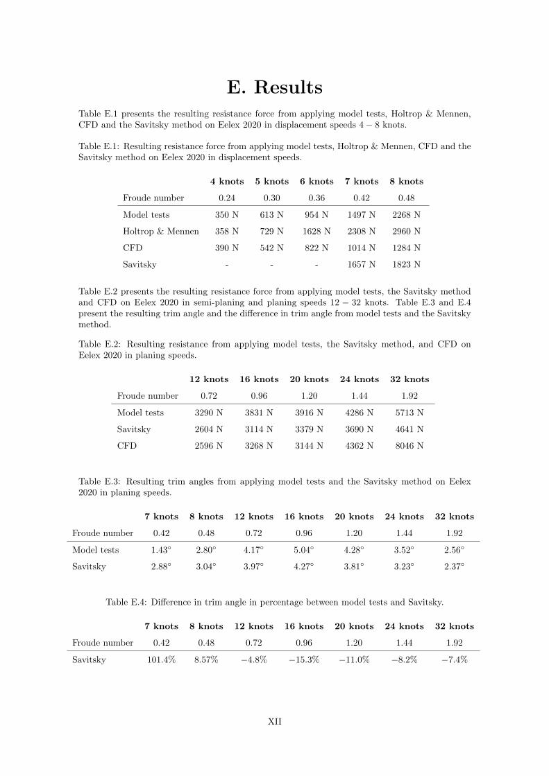
E. ResultsTable E.1 presents the resulting resistance force from applying model tests, Holtrop & Mennen,CFD and the Savitsky method on Eelex 2020 in displacement speeds 4− 8 knots.

Table E.1: Resulting resistance force from applying model tests, Holtrop & Mennen, CFD and theSavitsky method on Eelex 2020 in displacement speeds.

4 knots 5 knots 6 knots 7 knots 8 knots

Froude number 0.24 0.30 0.36 0.42 0.48

Model tests 350 N 613 N 954 N 1497 N 2268 N

Holtrop & Mennen 358 N 729 N 1628 N 2308 N 2960 N

CFD 390 N 542 N 822 N 1014 N 1284 N

Savitsky - - - 1657 N 1823 N

Table E.2 presents the resulting resistance force from applying model tests, the Savitsky methodand CFD on Eelex 2020 in semi-planing and planing speeds 12 − 32 knots. Table E.3 and E.4present the resulting trim angle and the difference in trim angle from model tests and the Savitskymethod.

Table E.2: Resulting resistance from applying model tests, the Savitsky method, and CFD onEelex 2020 in planing speeds.

12 knots 16 knots 20 knots 24 knots 32 knots

Froude number 0.72 0.96 1.20 1.44 1.92

Model tests 3290 N 3831 N 3916 N 4286 N 5713 N

Savitsky 2604 N 3114 N 3379 N 3690 N 4641 N

CFD 2596 N 3268 N 3144 N 4362 N 8046 N

Table E.3: Resulting trim angles from applying model tests and the Savitsky method on Eelex2020 in planing speeds.

7 knots 8 knots 12 knots 16 knots 20 knots 24 knots 32 knots

Froude number 0.42 0.48 0.72 0.96 1.20 1.44 1.92

Model tests 1.43◦ 2.80◦ 4.17◦ 5.04◦ 4.28◦ 3.52◦ 2.56◦

Savitsky 2.88◦ 3.04◦ 3.97◦ 4.27◦ 3.81◦ 3.23◦ 2.37◦

Table E.4: Difference in trim angle in percentage between model tests and Savitsky.

7 knots 8 knots 12 knots 16 knots 20 knots 24 knots 32 knots

Froude number 0.42 0.48 0.72 0.96 1.20 1.44 1.92

Savitsky 101.4% 8.57% −4.8% −15.3% −11.0% −8.2% −7.4%

XII

F. Modifying and combining methods

F.1 Modifying the Savitsky method with a correction factor

By adding a correction factor of 1.1758 to the total resistance from the Savitsky method, theaccuracy of the method is improved, see figure F.1.

Figure F.1: Resulting resistance force from the modified Savitsky method compared to the modeltests for Eelex 2020.

F.2 Combining CFD and the Savitsky method

The estimated values for trim angles and draught from the Savitsky method were used in the CFDsimulations in order to investigate if the accuracy of the resistance predictions could be improved.The trim angle was implemented in the CAD file, where the hull was rotated around the coordinatesystem. The same computational domain, mesh and setup as in the simulations without trim angleswere used. The free surface was located to generate a draught at transom corresponding to thevalues presented in table F.1. The simulations were made for two different speeds, 12 knots and32 knots.

Table F.1: Values used in the CFD simulations with trim angles.

Speed Trim angleDraught at

transomConverged

12 knots 3.97◦ 0.55 m No

32 knots 2.37◦ 0.28 m No

None of the simulations with implemented trim converged, and for 32 knots, an error indicatinga too coarse mesh appeared. To combine CFD and the Savitsky method, another mesh and/orsetup is required.

XIII

TRITA TRITA-SCI-GRU 2020:185

www.kth.se