methods for 3-d vector microcavity problems involving a...
TRANSCRIPT

Methods for 3-D vector microcavityproblems involving a planar dielectric
mirror
David H. Foster and Jens U. Nockel
Department of Physics
University of Oregon
Eugene, OR 97403
http://darkwing.uoregon.edu/~noeckel
Published in Optics Communications 234, 351-383 (2004)
We develop and demonstrate two numerical methods for solving the classof open cavity problems which involve a curved, cylindrically symmetric con-ducting mirror facing a planar dielectric stack. Such dome-shaped cavitiesare useful due to their tight focusing of light onto the flat surface. The firstmethod uses the Bessel wave basis. From this method evolves a two-basismethod, which ultimately uses a multipole basis. Each method is developedfor both the scalar field and the electromagnetic vector field and explicit“end user” formulas are given. All of these methods characterize the ar-bitrary dielectric stack mirror entirely by its 2 × 2 transfer matrices for s-and p-polarization. We explain both theoretical and practical limitations toour method. Non-trivial demonstrations are gi ven, including one of a stack-induced effect (the mixing of near-degenerate Laguerre-Gaussian modes) thatmay persist arbitrarily far into the paraxial limit. Cavities as large as 50λare treated, far exceeding any vectorial solutions previously reported.
Contents
1. Introduction 3
2. Overview of the Model and Notation 5
1

3. Plane Wave Bases and the Bessel Wave Method 83.1. The Field Expansion in the Simple Plane Wave Bases . . . . . . . . . . . 8
3.1.1. Scalar basis . . . . . . . . . . . . . . . . . . . . . . . . . . . . . . 83.1.2. Vector basis . . . . . . . . . . . . . . . . . . . . . . . . . . . . . . 10
3.2. The Field Expansion in the Bessel Wave Bases . . . . . . . . . . . . . . . 123.2.1. Scalar basis . . . . . . . . . . . . . . . . . . . . . . . . . . . . . . 123.2.2. Vector basis . . . . . . . . . . . . . . . . . . . . . . . . . . . . . . 14
3.3. The Linear System of Equations for the PWB . . . . . . . . . . . . . . . 163.3.1. The planar mirror (M1) boundary equations . . . . . . . . . . . . 163.3.2. The curved mirror (M2) boundary equations . . . . . . . . . . . 173.3.3. The seed equation . . . . . . . . . . . . . . . . . . . . . . . . . . 193.3.4. Solution of Ay=b . . . . . . . . . . . . . . . . . . . . . . . . . . . 193.3.5. Calculating the field from y . . . . . . . . . . . . . . . . . . . . . 19
4. Multipole Bases and the Two-Basis Method 204.1. The Scalar Multipole Basis . . . . . . . . . . . . . . . . . . . . . . . . . . 214.2. The M1 Equations in the Scalar MB . . . . . . . . . . . . . . . . . . . . 21
4.2.1. Variant 1 . . . . . . . . . . . . . . . . . . . . . . . . . . . . . . . 224.2.2. Variant 2 . . . . . . . . . . . . . . . . . . . . . . . . . . . . . . . 22
4.3. The Linear System of Equations in the Scalar MB . . . . . . . . . . . . . 234.4. Calculating the Field in the Layers with the Scalar MB . . . . . . . . . . 244.5. The Vector Multipole Basis . . . . . . . . . . . . . . . . . . . . . . . . . 244.6. The M1 Equations in the Vector MB . . . . . . . . . . . . . . . . . . . . 25
4.6.1. The M1 equations for s-polarization . . . . . . . . . . . . . . . . . 274.6.2. The M1 equations for p-polarization . . . . . . . . . . . . . . . . 274.6.3. Variant 1 . . . . . . . . . . . . . . . . . . . . . . . . . . . . . . . 284.6.4. Variant 2 . . . . . . . . . . . . . . . . . . . . . . . . . . . . . . . 28
4.7. The Linear System of Equations in the Vector MB . . . . . . . . . . . . . 294.8. Calculating the Field in the Layers with the Vector MB . . . . . . . . . . 30
5. Demonstrations and Comparisons 305.1. The “V” Mode: A Stack Effect . . . . . . . . . . . . . . . . . . . . . . . 305.2. Persistent Stack-Induced Mixing of Near-Degenerate Laguerre-Gaussian
Mode Pairs . . . . . . . . . . . . . . . . . . . . . . . . . . . . . . . . . . 325.2.1. Paraxial Theory for Vector Fields . . . . . . . . . . . . . . . . . . 335.2.2. A demonstration of persistent mixing . . . . . . . . . . . . . . . . 35
5.3. Modes with m 6= 1 . . . . . . . . . . . . . . . . . . . . . . . . . . . . . . 375.4. Ndirs and lmax: Comparing the Two Primary Methods . . . . . . . . . . . 385.5. Almost-Real MB Coefficients . . . . . . . . . . . . . . . . . . . . . . . . . 41
6. Conclusions 42
2

A. Further Explanations and Limitations of the Model 44A.1. Exclusion of High-Angle Plane Waves . . . . . . . . . . . . . . . . . . . 44A.2. The Hat Brim . . . . . . . . . . . . . . . . . . . . . . . . . . . . . . . . 44
A.2.1. The infinitesimal hat brim . . . . . . . . . . . . . . . . . . . . . . 44A.2.2. The infinite hat brim and the 1-D half-plane cavity . . . . . . . . 45
B. Negative m Modes and Sine and Cosine Modes 46B.1. Plotting with -m . . . . . . . . . . . . . . . . . . . . . . . . . . . . . . . 46B.2. Plotting cosine and sine modes . . . . . . . . . . . . . . . . . . . . . . . 47
C. Stacks used in Section 5 48
1. Introduction
There is currently considerable interest in the nature of electromagnetic (vector) modesboth for free space propagation [1, 2, 3, 4] and in cavity resonators [5]. In particular,recent advances in fabrication technology have given rise to optical cavities which cannotbe modeled by effectively two-dimensional, scalar or pseudo-vectorial wave equations [6].The resulting modes may exhibit non-paraxial structure and nontrivial polarization, butthis added complexity also gives rise to desirable effects; an example from free-spaceoptics is the observation of enhanced focusing for radially polarized beams [4]. Thiseffect is shown here to arise in cavities as well, among a rich variety of other modes thatdepend on the three-dimensional geometry. The main goal of this paper is to present aset of numerical techniques adapted to a realistic cavity design as described below.
Much work involving optical cavity resonators utilizes mirrors that are composed ofthin layers of dielectric material. These dielectric stack mirrors offer both high reflectivityand a low ratio of loss to transmission, which are desirable in many applications. Thesimplest model of such cavities treats the mirrors as perfect conductors (Etangential =0, Hnormal = 0). In applications involving paraxial modes and highly reflective mirrors,it is often acceptable to use this treatment. The mature theory of Gaussian modes (c.f.Siegman [7]) is applicable for this class of cavity resonator. When an application requiresgoing beyond the paraxial approximation to describe the optical modes of interest, theproblem becomes significantly more involved and modeling dielectric stack mirrors asconducting mirrors may become a poor approximation. Also, one is often interested inthe field inside the dielectric stack and for this reason must include the stack structureinto the problem.
In this paper we present a group of improved methods for resonators with a cylin-drically symmetric curved mirror facing a planar mirror. The paraxial condition is notnecessary for these methods; tightly focused modes can be studied. Furthermore, thetrue vector electromagnetic field is used, rather than a scalar field approximation. Theplanar mirror is treated as infinite and is characterized by its polarization-dependentreflection functions rs(θinc) and rp(θinc) for plane waves with incident angle θinc. Ourmodel encompasses both cavities for which the planar mirror is an arbitrary dielectric
3
stack, and cavities for which the planar mirror is a simple mirror (conducting withrs/p(θinc) = −1 or “free” with rs/p(θinc) = +1). The opposing curved mirror is alwaystreated as a conductor. It should be noted that, for most modes which are highly fo-cused at the planar mirror, (modes which are likely to be of interest in applications),this limitation can be expected to cause little error because the local wave fronts at thecurved mirror are mostly perpendicular to its surface. (Of course, for applications inwhich the curved mirror is indeed conducting, our model is very well suited.) On theother hand, the correct treatment of the planar mirror can be a great improvement overthe simplest model. Applications with both dielectric and conducting curved mirrorshave been and are currently being used experimentally [5, 8, 9].
The methods described here belong to a class of methods which we refer to as “basisexpansion methods”. In basis expansion methods, a complete, orthogonal basis (suchas the basis of electromagnetic plane waves) is chosen. Each basis function itself obeysMaxwell’s equations. The equations that determine the correct value of the basis coef-ficients are boundary equations, resulting from matching appropriate fields at dielectricinterfaces, setting appropriate field components to zero at conductor-dielectric interfaces,and setting certain fields to be zero at the origin or infinity. In the usual application ofthis method, each homogenous dielectric region is allocated its own set of basis coeffi-cients. Our methods use a single set of basis coefficients; the matching between dielectriclayers is handled by the 2× 2 transfer matrices of the stack.
As dielectric stacks have nonzero transmission, optical cavities with this type of mirrorare necessarily open, or lossy. The methods described here deal with the openness due tothe stack and the solutions are quasimodes, with discrete, isolated complex wavenumberswhich denote both the optimal driving frequency and the resonance width1. Whilethe dielectric mirror is partially responsible for the openness of our model system, theopenness is not primarily responsible for mode pattern changes resulting from replacinga dielectric stack mirror with a simple mirror. The phase shifts of plane waves reflectedoff a dielectric stack can vary with incident angle, and it is this variation which cancause significant changes in the modes, even though reflectivities may be greater than0.99. Generally speaking, the deviation of |rs/p(θinc)| from 1 is not as important as thedeviation of arg(rs/p(θinc)) from, say, arg(rs/p(0)).
We develop two general methods, the two-basis method and the Bessel wave method.The scalar field versions of both methods are also developed and are discussed first, actingas pedagogical stepping stones to the vector field versions. The Bessel wave method usesthe Bessel wave basis which is the cylindrically symmetric version of the plane wave basis.This method is described in Section 3. The two-basis method ultimately uses the vectoror scalar multipole basis. The multipole basis has an advantage in that it is the eigenbasisof a conducting hemisphere, the “canonical” dome-shaped cavity. The unusual aspect of
1For many modes, there is also loss due to lateral escape from the sides of the cavity. While our modelintrinsically incorporates the openness due to lateral escape in the calculation of the fields (by simplynot closing the curved mirror surface, or extending its edge into the dielectric stack), this loss is notincluded in the calculated resonance width or quality factor, Q. Because a single set of basis vectorsis used to describe the field in the half-plane above the planar mirror, this entire half-plane is the“cavity” as far as the calculation of resonance width is concerned.
4

the two-basis method is the intermediate use of the Bessel wave basis. The two-basismethod is developed in Section 4. We have implemented both methods and have usedthem as numerical checks against each other. Various demonstrations and comparisonsare given in Section 5. Our implementations of all methods are programmed in C++, usethe GSL, LAPACK, SLATEC, and PGPlot numerical libraries, and run on a MacintoshG4 with OS X. Limitations of our model and methods are discussed in Appendix A.Appendix B discusses plotting modes that are associated with linear polarization andAppendix C specifies dielectric stacks that are used in Section 5.
2. Overview of the Model and Notation
Figure 1: The cavity model.
A diagram of the model is shown in Figure 1. The conducting surface is indicated bythe heavy line. The annular portion of this surface extending horizontally from the domeedge will be referred to as the “hat brim”. The dome is cylindrically symmetric withmaximum height z = R and edge height z = ze. The shape of the dome is arbitrary,but in our demonstrations the dome will be a part of an origin-centered sphere of radiusRs = R unless otherwise specified. The region surrounding the curved mirror will bereferred to as layer 0. The dielectric interface between layer 0 and layer 1 has heightz = z1. The last layer of the dielectric stack is layer N and the exit layer is called layerX. The depiction of the stack layers in the figure suggests a design in which the stackconsists of some layers of experimental interest (perhaps containing quantum wells, dots,or other structures [5, 8]) at the top of the stack where the field intensity is high, and ahighly reflective periodic structure below.
5

At the heart of the procedure to solve for the quasimodes is an overdetermined, com-plex linear system of equations, Ay = b. The column vector y is made up of thecoefficients of eigenmodes in some basis B. The field in layer 0 is given by expansion inB using these coefficients. For a given wavenumber, k, a solution vector y = ybest canbe found so that |A(k) y − b|2 is minimized with respect to y. Dips in the graph of theresidual quantity, ∆r ≡ |A(k) ybest − b|, versus k signify the locations of the isolatedeigenvalues of k (theoretically ∆r should become 0 at the eigenvalues). The solutionvector ybest(k) at one of these eigenvalues describes a quasimode. The system of equa-tions is made up of three parts (as shown below): M1 equations, M2 equations and anarbitrary amplitude or “seed” equation.
Ay =
[
M1
][
M2
][s. eqn.
]
·
y
=
0...
...01
. (1)
Henceforth M1 refers to the planar mirror and M2 to the curved mirror.The M1 boundary condition for a plane wave basis is expressed simply in terms of
the 2 × 2 stack transfer matrices Ts(θinc) and Tp(θinc), as suggested by the M1 region(enclosed by the dashed line) in Fig. 1. In the scalar and vector multipole bases, a sortof conversion to plane waves is required as an intermediate step. The dashed k vectorsin the figure (incoming from the bottom of the stack) represent plane waves that aregiven zero amplitude, in order to define a quasimode problem rather than a scatteringproblem. The plane waves denoted by the solid k vectors have nonzero amplitude.
The M2 boundary condition is implemented as follows. A number of locations on thecurved mirror are chosen (the “X” marks in Fig. 1). The width of the hat brim is wb asshown. An“infinitesimal”hat brim (wb λ) is introduced to give the dome a diffractiveedge. An “infinite” hat brim can be introduced theoretically and can make the modelmore easily understandable in certain respects. More about the model in relation to thehat brim is discussed in Appendix A.2. The M2 equations are the equations in basis Bsetting the appropriate fields at these locations to zero. For a problem not possessingcylindrical symmetry, these locations would be points. The simplification due to thissymmetry, however, allows these locations to be entire rings about the z axis, specifiedby a single parameter such as the ρ coordinate. Finally, the seed equation sets somecombination of basis coefficients equal to one and is the only equation with a nonzerovalue on the right hand side (b).
The cylindrical symmetry of the boundary conditions allows one to always find solu-tions which have a φ dependence of exp(ımφ), where m is an integer. This in turn leadsto a dimensionally reduced version of the plane wave basis called the Bessel wave basis,in which each basis function is a superposition of all the plane waves with the samewavevector polar angle, θk. The weight function of the superposition is proportional toexp(ımφk). We will refer to the non-reduced basis as the “simple plane wave basis”. The
6

unadorned phrase “plane wave basis” (PWB; same abbreviation for plural) will referhenceforth to either or both of the Bessel wave and simple plane wave bases. Whenusing the scalar or vector multipole basis (MB; same abbreviation for plural), cylindricalsymmetry allows the problem to be solved separately for each quantum number m ofinterest2. The dimensional reduction in this case amounts to the removal of a summationover m in the basis expansion.
The refractive index in region (layer) q is denoted nq. Layers are also denoted with anupper subscript in parenthesis: E(q) means the electric vector field in layer q. Sometimes“fs” is used as a value of q, meaning “in free space” (e.g. nfs), whether or not any of thelayers in the model we are considering actually are free space. We note here that nfs = 1only in “cavity type I” discussed below.
The symbol k, where not in a super/subscript and not bold nor having any su-per/subscripts, always refers to what may be called the “wavenumber in free space”,although it will have an imaginary part if M1 is a dielectric mirror. An imaginary partin wavenumber, refractive index, and/or frequency is often introduced (as it is in thisproblem) to turn open cavity problems into eigenvalue problems. The definition of k isas follows. Define −k2
q as the constant of separation used to separate space and timeequations from the wave equation for layer q:
∇2X(q) =n2
q
c2∂2X(q)
∂t2. (2)
Here X(q) may be a vector or scalar field. In a few steps, the selection of a globalmonochromatic time dependence exp(−ıωt) reveals that the ratio kq/nq is independentof q. Then k is defined as k ≡ kfs, so that kq = nqk where nq ≡ nq/nfs. In the model,the index ratios nq are assumed to be real. The single plane wave solution to (2) has the
form X(q) = C(q)eık(q)·xe−ıωt where C(q) is a constant vector or scalar and the complexwave vector k(q) is given by k(q) ≡ kqΩ
(q)k = knqΩ
(q)k with Ω
(q)k being the unit direction
vector of the plane wave, specified by θ(q)k and φk. The generally complex frequency is
given by ω = ckq/nq. At a refractive interface, the angle θ(q)k changes as given by Snell’s
law.To understand the meaning of a complex k, it is helpful to realize that the spatial
dependence of the quasimodes are identical3 in the following two physical cavities:
I : nfs = 1, nq = nq,
II : nfs = Υ, nq = Υnq,Υ ∈ C. (3)
2The modes with low |m| are likely to be of practical interest since they have the simplest transversepolarization structure. The |m| = 1 family of vector eigenmodes is exceptional because the pro-portionality of Eρ and Eφ to exp(ımφ) means that modes for |m| 6= 1 have no average transverseelectric field, even instantaneously. (It is straightforward to show that 〈ReEx〉φ = 〈ReEy〉φ = 0 if|m| 6= 1.) Thus a uniformly polarized, focused beam centered on the cavity axis can not couple tocavity modes with |m| 6= 1 !
3There is the minor difference for the magnetic field first noted in Eqn. (12). Since the discrepancyis a constant factor multiplying H, however, this difference is not necessarily part of the spatialdependence.
7

(The shape and size of each dielectric and conducting region are the same for cavitiesI and II.) Cavity I is composed of of conductors and zero-gain regions of real refractiveindex. Cavity II is constructed by taking cavity I and multiplying the refractive index ofeach region, including free space, by an arbitrary complex number Υ. The congruenceof the spatial quasimodes follows from separating the variables in (2). The values of k,kq, and nq for a given quasimode are the same in cavities I and II. The frequency incavity II is ωII = ωI/Υ. If we henceforth consider only the specific cavity II for which Υ= (1− ıg) where g is tuned to be the ratio (−Imk/Rek) (for a given quasimode), we seethat ωII = cRek = ReωI. While in cavity I the quasimode decays in time, in cavity IIthe quasimode is a steady state because the gain exactly offsets the loss. Either of thetwo cavity types may be imagined to be the case in our treatment. The only differenceis the existence of the decay factor exp(cIm(k)t) for cavity I. (The inequality Imk ≤ 0always turns up for an eigenvalue problem with conducting and/or dielectric interfaceboundary conditions.) We note that the relation of k to the free space wavelength (alwaysreal) of a plane wave is k = (1 − ıg)2π/λ. The quality factor, Q, of the quasimode isRek/(2|Imk|) = 1/(2g).
We note that Snell’s law, nq sin θ(q)k = nq+1 sin θ
(q+1)k , is independent of whether we
have a cavity of type I or II because the quantity (1 − ıg), if present, divides out. Oneof the limitations of our method is the omission of evanescent waves in layer 0 andin layers where nq ≥ n0 (see Appendix A.1). Snell’s law may cause θ
(q)k to become
complex for layers with index ratios nq less than n0. In this case sin θ(q)k > 1 and
cos θ(q)k = ısgn(cos θ
(0)k )[sin2 θ
(q)k − 1]1/2.
In most cases the symbols ψ, E, and H stand for complex-valued fields. The timedependence is exp(−ıωt) and it is usually suppressed. Physical fields are obtained bymultiplying by the time dependence and then taking the real part.
Throughout this paper, the common functions denoted by Ylm, Pml , Pl, Jn, jl, and nl
are defined as they are in the book by Jackson [10].In the implementation, c and the related constants ε0, µ0, and Z0 are all unity, and
they will usually be dropped in our treatment. We also assume non-magnetic materialsso that µq = µ0 = 1.
3. Plane Wave Bases and the Bessel Wave Method
Although this major section describes the Bessel wave method, much of what is discussedhere is applicable to the two-basis method with little alteration. The discussion in Section4 is greatly shortened due to this overlap of concepts and procedures.
3.1. The Field Expansion in the Simple Plane Wave Bases
3.1.1. Scalar basis
A single scalar plane wave in layer q has the form ψ = C exp (ık(q) · x− ıωt). For ageneral monochromatic field, k and ω are fixed and the field can be expressed (due to
8
the completeness of the scalar PWB) uniquely (due to the orthogonality of the scalarPWB) as a sum over plane waves in different directions. In our treatment however, weomit plane waves in layer q which would only exist as evanescent waves when refractedinto layer 0. The expansion for the field in layer q is
ψ(q)(x) =
∫ 2π
0
dφk
∫ π
0
dθ(0)k sin(θ
(0)k )ψ
(q)k eık(q)·x. (4)
Here the basis expansion coefficients are the ψ(q)k (continuous coefficients in the integral,
and discrete coefficients in implementation). The above expansion effectively propagateseach plane wave existing in the cavity down (whether forward or backward) into the stack
layers, and adds up all of their contributions. In order to express the ψ(q)k in terms of
ψ(0)k , it is first necessary to separate the coefficients with kz > 0 from those with kz < 0
and write the above expansion as
ψ(q) =
∫ 2π
0
dφk
∫ π/2
0
dα(0)k sin(α
(0)k )
×(ψ(q)
u eık(q)u ·x + ψ
(q)d eık
(q)d ·x). (5)
The u and d refer to the plane waves going upward or downward, e.i. ψ(q)u is the expansion
coefficient ψ(q)k for k
(q)z > 0 (or k
(0)z > 0, since sgn(k
(q)z ) = sgn(k
(0)z )) and ψ
(q)d takes the
place of ψ(q)k for k
(0)z < 0. The wavevector k(q) in cylindrical coordinates is (k
(q)ρ , k
(q)φ , k
(q)z ),
for which the following relationships hold:
k(q)ρ = kq sin θ
(q)k = kn0 sin θ
(0)k = kn0 sinα
(0)k = k(0)
ρ ,
k(q)z = kq cos θ
(q)k = knqsgn(cos θ
(0)k ) cosα
(q)k
= knqsgn(cos θ(0)k )
√1−
(n0
nq
sinα(0)k
)2
,
k(q)φ = φk (indep. of q). (6)
This leads to
ψ(q) =
∫ 2π
0
dφk
∫ π/2
0
dα(0)k sin(α
(0)k )eıϕρ
×(ψ(q)
u eıϕz + ψ(q)d e−ıϕz
), (7)
where
ϕρ ≡ ρkn0 sin(α(0)k ) cos(φ− φk),
ϕz ≡ zknq cosα(q)k . (8)
9

From standard theory regarding plane waves and layered media[11], one can calculate
the 2 × 2 complex transfer matrix, T(q)s , that obeys the following equation(
ψ(q)d e−ıϕz
ψ(q)u eıϕz
)= T (q)
s ·(ψ
(0)d
ψ(0)u
). (9)
Defining the column sums +β(q)s ≡ T
(q)s,12 + T
(q)s,22 and +γ
(q)s ≡ T
(q)s,11 + T
(q)s,21 allows us to
write the expansion of the scalar wave in the layers as
ψ(q) =
∫ 2π
0
dφk
∫ π/2
0
dα(0)k sin(α
(0)k )
× eıϕρ
(+β
(q)s ψ(0)
u + +γ(q)s ψ
(0)d
). (10)
The reason for the notation with the subscripts “+” and “s” will become apparent in thevector discussion. The “s” refers to s-polarization.
The variables in the simple PWB for scalar fields are the complex ψ(0)u and ψ
(0)d (the
superscript will often be dropped). Next we consider the simple PWB for vector fields.
3.1.2. Vector basis
We assume that for our purposes a general monochromatic electromagnetic field can beexpressed uniquely as a sum of vector (electromagnetic) plane waves. For every givenfrequency and wavevector direction Ωk there are two orthogonally polarized plane waves(as opposed to a single plane wave in the scalar case). Instead of a single coefficient ψk foreach spatial direction we need two, Sk and Pk, which we can define as follows. Sk is theamplitude of the vector plane wave propagating in direction Ωk which has its electricfield polarized in the x-y plane (Ez = 0). Thus, this plane wave is an “s-wave” withregard to the planar mirror. Pk is the amplitude of the “p-wave”, the vector plane wavein direction Ωk which has its electric field polarized in the plane of incidence (Eφ = 0).The coefficients Sk and Pk will be separated into Su, Sd, Pu, and Pd.
To specify the polarization of the fields we will use unit vectors denoted by ε. Theunit vector ε
(q)s,k denotes the direction of the electric field associated with the plane wave
with wavevector k(q) and s-polarization. We take the direction of the unit vectors to be:
ε(q)s,k = −φk
= x sinφk − y cosφk,
ε(q)p,k = θ
(q)k sgn(cos θ
(q)k )
= ρksgn(cos θ(0)k ) cos θ
(q)k − zsgn(cos θ
(0)k ) sin θ
(q)k . (11)
In this phase convention (used by Yeh[11]), the projections of the ε(q)p,k vectors for the
incident and reflected waves onto the x-y plane are equal. The other common phaseconvention has these projections being in opposite directions.
10

The entire electric and magnetic field can be broken up into two parts: E(q) = E(q)s +
E(q)p and H(q) = H
(q)s + H
(q)p where H
(q)s is the field with magnetic s-polarization
(Hz = 0) and H(q)p is the field with magnetic p-polarization (Hφ = 0). We can now
write down the most compact expansion of the vector field.
E(q)s =
∫dΩ
(0)k S
(q)k ε
(q)s,ke
ık(q)·x,
E(q)p =
∫dΩ
(0)k P
(q)k ε
(q)p,ke
ık(q)·x,
H(q)s = −nq
∫dΩ
(0)k P
(q)k ε
(q)s,ksgn(cos θ
(0)k )eık(q)·x,
H(q)p = nq
∫dΩ
(0)k S
(q)k ε
(q)p,ksgn(cos θ
(0)k )eık(q)·x. (12)
The factors of nq in the H equations come from the physical relation of H to E for aplane wave. Note that nq is different for cavity types I and II (as given in Eqn. (3)).Separating up and down coefficients yields
E(q)s =
∫ 2π
0
dφk ε(q)s,k
∫ π/2
0
dα(0)k sin(α
(0)k )eıϕρ
×(S(q)
u eıϕz + S(q)d e−ıϕz
),
E(q)p =
∫ 2π
0
dφk
∫ π/2
0
dα(0)k sin(α
(0)k ) eıϕρ
×[ρk cos(α
(q)k )(P (q)
u eıϕz + P(q)d e−ıϕz
)+ z sin(α
(q)k )(−P (q)
u eıϕz + P(q)d e−ıϕz
)]. (13)
These expressions explicitly use coordinate vectors only where necessary due to a de-pendence of the εk vectors on the sign of cos θ
(0)k . The expressions for H(q) are omitted
for brevity.To relate S
(q)u/d and P
(q)u/d to S
(0)u/d and P
(0)u/d we can use the transfer matrices: Ts for
s-polarized light and Tp for p-polarized light. The transfer matrix used for the scalarfield in Eqn. (9) is the same matrix we will use here for s-polarization. These matricesperform the following transformations(
S(q)d e−ıϕz
S(q)u eıϕz
)= T (q)
s ·(S
(0)d
S(0)u
),(
P(q)d e−ıϕz
P(q)u eıϕz
)= T (q)
p ·(P
(0)d
P(0)u
). (14)
We define
±β(q)s ≡ T
(q)s,12 ± T
(q)s,22,
±γ(q)s ≡ T
(q)s,21 ± T
(q)s,11,
11

±β(q)p ≡ T
(q)p,12 ± T
(q)p,22,
±γ(q)p ≡ T
(q)p,21 ± T
(q)p,11. (15)
Note +β(q)s and +γ
(q)s are defined as before. The β and γ quantities are functions of z
and z1 and not of ρ or φ. They are functions of k and α(0)k but not of φk.
Now the field expansions become
E(q)s =
∫ 2π
0
dφk ε(q)s,k
∫ π/2
0
dα(0)k sin(α
(0)k )eıϕρ
×(
+β(q)s S(0)
u + +γ(q)s S
(0)d
),
E(q)p =
∫ 2π
0
dφk
∫ π/2
0
dα(0)k sin(α
(0)k ) eıϕρ
×[ρk cos(α
(q)k )(
+β(q)p P (0)
u + +γ(q)p P
(0)d
)+ z sin(α
(q)k )(−β
(q)p P (0)
u − −γ(q)p P
(0)d
)],
H(q)s = nq
∫ 2π
0
dφk ε(q)s,k
∫ π/2
0
dα(0)k sin(α
(0)k )eıϕρ
×(−β
(q)p P (0)
u − −γ(q)p P
(0)d
),
H(q)p = nq
∫ 2π
0
dφk
∫ π/2
0
dα(0)k sin(α
(0)k ) eıϕρ
×[ρk cos(α
(q)k )(− −β
(q)s S(0)
u + −γ(q)s S
(0)d
)− z sin(α
(q)k )(
+β(q)s S(0)
u + +γ(q)s S
(0)d
)]. (16)
The variables in the simple PWB for vector fields are the complex S(0)u , S
(0)d , P
(0)u , and
P(0)d (the superscript will often be dropped).
3.2. The Field Expansion in the Bessel Wave Bases
3.2.1. Scalar basis
We have already assumed a time dependence of exp(−ıωt). As mentioned in the Overview,a cylindrically symmetric set of boundary conditions allows us to assume an azimuthaldependence of exp(ımφ) with m being an integer. Consider the expansion (4). We wish
to find the conditions on ψ(q)k which cause the entire dependence of ψ(x) on φ to be
exp(ımφ).
The general Fourier series expansion of ψ(q)k is
ψ(q)k (θ
(0)k , φk) =
∑n
f (q)n (θ
(0)k ) eınφk . (17)
12

We can then write (4) as
ψ(q) =∑
n
∫ π
0
dθ(0)k sin(θ
(0)k )eıϕzf (q)
n (θ(0)k )
×∫ 2π
0
dφk eıρkn0 sin(θ
(0)k ) cos(φ−φk)eınφk , (18)
where
ϕz ≡ zknq cos θ(q)k . (19)
The last integral is of the solved form∫ 2π
0
eıy cos(φ′−φ)eınφ
′
dφ′= 2π(ı)nJn(y)eınφ, (20)
where Jn denotes the regular Bessel function of order n (n can be negative). This yields
ψ(q) = 2π∑
n
(ı)neınφ
∫ π
0
dθ(0)k sin(θ
(0)k )
× eıϕzJn(ρkn0 sin θ(0)k )f (q)
n (θ(0)k ). (21)
In order to have only exp(ımφ) dependence on φ, the integral on the right hand side
must be zero for n 6= m. Because f(q)n (θ
(0)k ) cannot be a function of z or ρ, the only way to
have this for all z and ρ is to pick fn = 0 for n 6= m. Thus ψ(q)k (θ
(0)k , φk) = f
(q)m (θ
(0)k )eımφk .
At this point we define the symbol ψ(q)k to mean the coefficient f
(q)m . The cylindrically
symmetric expansion is
ψ(q) = ξ
∫ π
0
dθ(0)k sin(θ
(0)k )eıϕzJm(ρkn0 sin θ
(0)k )ψ
(q)k (θ
(0)k ), (22)
where
ξ ≡ 2π(ı)meımφ. (23)
This is an expansion in scalar Bessel waves, defined to be
ξ exp(ızknq cos θ(q)k )Jm(ρkn0 sin θ
(0)k ), (24)
with ψ(q)k (θ
(0)k ) being the set of coefficients. Each Bessel wave is a set of simple plane
waves with fixed polar angle but having the full range (0 to 2π) of azimuthal angles,φk. The weight factors of the plane waves are proportional to exp(ımφk). The finalcylindrically symmetric scalar expansion with up and down separated is
ψ(q)(x) = ξ
∫ π/2
0
dα(0)k sin(α
(0)k )Jm(ρkn0 sinα
(0)k )
×(
+β(q)s ψ(0)
u + +γ(q)s ψ
(0)d
). (25)
The ψ(0)u and ψ
(0)d are the (complex) variables in the Bessel wave method for scalar fields;
they make up the solution vector y in (1).
13
3.2.2. Vector basis
For cylindrically symmetric boundary conditions, the φ dependence of Eρ, Ez, Eφ, Hρ,Hz, and Hφ can be taken (for a single mode) to be exp(ımφ).
Consider doing the φk integrations in (12) or (16). The unit vectors ε(q)s/p,k and ρk
depend on φk. The z components do not depend on φk so we will look at these first.There is no contribution to the z component of the electric field from E
(q)s nor is there
any contribution to the z component of the magnetic field from H(q)s . We define
zP(q)(x) ≡ E(q) · z = E(q)
p · z,HzP
(q)(x) ≡ H(q) · z = H(q)p · z. (26)
Requiring that these quantities have an exp(ımφ) dependence produces results similarto the scalar case. Defining
S(q)k eımφk ≡ S
(q)k ,
P(q)k eımφk ≡ P
(q)k , (27)
and using (16), we have the final, useful expansions for zP(q) and H
zP(q):
zP(q) = ξ
∫ π/2
0
dα(0)k sin(α
(0)k ) sin(α
(q)k )
× Jm(ρkn0 sinα(0)k )(−β
(q)p P (0)
u − −γ(q)p P
(0)d
),
HzP
(q) = − ξnq
∫ π/2
0
dα(0)k sin(α
(0)k ) sin(α
(q)k )
× Jm(ρkn0 sinα(0)k )(
+β(q)s S(0)
u + +γ(q)s S
(0)d
). (28)
To deal with the transverse part of the electromagnetic field it is helpful to use quan-tities related to circular polarization. We define
±S(q) ≡ ±ıE(q)
s · x−E(q)s · y
= e±ıφ(±ıE(q)s · ρ−E(q)
s · φ),H±S
(q) ≡ ±ıH(q)s · x−H (q)
s · y
= e±ıφ(±ıH (q)s · ρ−H (q)
s · φ),
±P(q) ≡ E(q)
p · x± ıE(q)p · y
= e±ıφ(E(q)p · ρ± ıE(q)
p · φ),H±P
(q) ≡ H(q)p · x± ıH(q)
p · y
= e±ıφ(H(q)p · ρ± ıH(q)
p · φ). (29)
Inverting (29) yields
E(q)s · ρ =
−ı2
( +S(q)e−ıφ − −S
(q)eıφ),
E(q)s · φ =
−1
2( +S
(q)e−ıφ + −S(q)eıφ),
14

E(q)p · ρ =
1
2( +P
(q)e−ıφ + −P(q)eıφ),
E(q)p · φ =
−ı2
( +P(q)e−ıφ − −P
(q)eıφ), (30)
with the magnetic field quantities having similar relations. Now we use (12) and (11)with (29). The resulting electric field quantities are
±S(q) =
∫ π
0
dθ(0)k sin(θ
(0)k )eıϕz
×∫ 2π
0
dφke±ıφkeıρkn0 sin(θ
(0)k ) cos(φ−φk)S
(q)k ,
±P(q) =
∫ π
0
dθ(0)k sin(θ
(0)k ) cos(θ
(q)k )sgn(cos θ
(0)k )eıϕz
×∫ 2π
0
dφke±ıφkeıρkn0 sin(θ
(0)k ) cos(φ−φk)P
(q)k . (31)
It is the exp(±ıφk) factors in the integrands here that motivated the definitions of ±S/P(29). We see that the substitution of (27) into (31) results in φk integrals of the form(20). Performing this substitution, doing the integrals, and separating the up and downparts gives the final expansions:
±S(q) = ξ±
∫ π/2
0
dα(0)k sin(α
(0)k )Jm±1(ρkn0 sinα
(0)k )
×(
+β(q)s S(0)
u + +γ(q)s S
(0)d
),
±P(q) = ξ±
∫ π/2
0
dα(0)k sin(α
(0)k )Jm±1(ρkn0 sinα
(0)k )
× cos(α(q)k )(
+β(q)p P (0)
u + +γ(q)p P
(0)d
),
H±S
(q) = ξ±nq
∫ π/2
0
dα(0)k sin(α
(0)k )Jm±1(ρkn0 sinα
(0)k )
×(−β
(q)p P (0)
u − −γ(q)p P
(0)d
),
H±P
(q) = ξ±nq
∫ π/2
0
dα(0)k sin(α
(0)k )Jm±1(ρkn0 sinα
(0)k )
× cos(α(q)k )(− −β
(q)s S(0)
u + −γ(s)s S
(0)d
), (32)
where
ξ± ≡ 2π(ı)m±1eı(m±1)φ. (33)
At this point one can quickly verify, using (30) and the above equations, that Eρ, Eφ,Hρ, and Hφ do indeed have a φ-dependence of exp(ımφ).
15

The S(0)u , S
(0)d , P
(0)u , and P
(0)d are the (complex) variables in the Bessel wave method and
make up the solution vector y in (1). They are essentially coefficients of electromagneticBessel waves, although we need not explicitly combine (32), (30), (28), and (26) to obtainan explicit expression for the E and H vector Bessel waves as we did for the scalar case(24).
3.3. The Linear System of Equations for the PWB
Until now the PWB coefficients have been treated as continuous, when in practice theymust be chosen discrete. Let us keep in mind this discrete nature in the followingsubsections. We denote by Ndirs the number of directions α
(0)k we choose. Thus there
are 2Ndirs coefficient variables for a scalar problem and 4Ndirs coefficient variables for avector problem. The distribution of the α
(0)k on [0, π/2] need not be uniform, and the
effect of distribution choice will be briefly mentioned later.
3.3.1. The planar mirror (M1) boundary equations
The M1 equations (planar mirror boundary condition equations) in the PWB are verysimple. In fact, because of this simplicity, the M1 equations in the MB are basically atransformation to and from the PWB with the M1 equations for the PWB sandwichedbetween. The reflection of a plane wave off of a layered potential is a well knownproblem. For the purpose of determining the field in layer 0, the entire dielectric stackis characterized by the complex rs and rp coefficients acting at the first surface of thestack. For the scalar case with the layer 0–layer 1 interface at z1 = 0, the boundarycondition is just ψ
(0)u = rs(α
(0)k )ψ
(0)d where rs(α) is the stack reflection function. Since
Bessel waves are linear superpositions of many plane waves with the same θ(0)k parameter,
this equations is true for Bessel waves:
ψ(0)u = rs(α
(0)k )ψ
(0)d . (34)
For a conducting mirror, set rs = −1 and for a free mirror set rs = 1.If the interface is at a general height z1, then the same rs function is used at this
surface yielding
ψ(0)u eız1kn0 cos α
(0)k = rs(α
(0)k )ψ
(0)d e−ız1kn0 cos α
(0)k ,
or
ψ(0)u − rs(α
(0)k )ψ
(0)d = 0, (35)
where
rs/p(α(0)k ) ≡ rs/p(α
(0)k )e−ı2z1kn0 cos α
(0)k . (36)
16

(The equation is given for both s- and p-polarization since we will shortly be using the
rp quantities.) The quantities rs/p(α(0)k ) are independent of z and z1. When M2 is a
dielectric stack mirror, the rs/p(α) are determined by T(q=layer X)s/p according to
rs/p(α) = −T (X)s/p,21/T
(X)s/p,22. (37)
For the vector case the equation for the s-polarized plane waves is
E(0)u · ε(0)
s,u = rs(α(0)k )E
(0)d · ε
(0)s,d, (38)
where E(0)u/d is the total electric field of the two plane waves going in the direction specified
by αk, φk, and u or d. Shifting to our current notation and to Bessel waves, the equationbecomes
S(0)u − rs(α
(0)k )S
(0)d = 0. (39)
For p-polarization there is an arbitrary conventional sign. In our phase convention(chosen in (11)) the equation is
E(0)u · ε(0)
p,u = rp(α(0)k )E
(0)d · ε
(0)p,d, (40)
or
P (0)u − rp(α
(0)k )P
(0)d = 0. (41)
The vector ε(0)p,u/d is ε
(0)
p,kwith k being k forced into the up/down version of itself.
For a simple mirror, set rp = rs = −1 for conducting, +1 for free and use (36)instead of (37) to determine rs/p. Sometimes we will use cosαk as the explicit argumentto rs/p or rs/p instead of αk.
Equation (35) or Eqns. (39) and (41), given for each discrete α(0)k , form the M1
equations.
3.3.2. The curved mirror (M2) boundary equations
As mentioned in Section 2, the M2 equations come from setting the appropriate fieldcomponents equal to zero at some number of locations on the curved mirror and the hatbrim. If we chose individual points on the two dimensional surface, the φ-dependencefactor, exp(ımφ), could be divided away. Thus picking locations with the same ρ and zbut different φ yields identical boundary equations. Therefore we simply set φ = 0 (andt = 0) and pick equations by incrementing a single parameter (such as ρ) on the onedimensional curve given by the intersection of the conducting mirror and the x-z plane.The number of locations, NM2 loc, determines the number of M2 boundary equations.All of the locations are taken to lie in layer 0.
We obtain the M2 equations by, in effect, doing the α(0)k integrals in (25) or in (28) and
(32). Before making the integrals discrete, the distribution of representative directions
17

must be chosen. If the interval ∆α(0)k between successive directions is not constant, the
integral over α(0)k must be transformed to an integral over a new variable, x, where ∆x
is constant. Such a transformation will generate a new integration factor. At this pointthe integral is turned into a sum according to:
∫ b
a→∑
j , dx → (b − a)/N . Choosing
the direction distribution to be uniform in α(0)k requires no change in integration factor
and yields a “summation factor” of π/(2Ndirs).Using (25) and (23), the M2 equations for the scalar problem are
2π
(π
2Ndirs
)Ndirs∑j=1
[Jm(ρ∗kn0 sinα
(0)kj
)
× sin(α(0)kj
)(
+β(0)s
∣∣z=z∗
ψuj+ +γ
(0)s
∣∣z=z∗
ψdj
)]= 0. (42)
An equation is added to the linear system for each chosen location specified by (ρ∗, z∗).All phase factors have been divided out of (42) but the scale factor π2/Ndirs has been keptfor representative weighting. Of course there is also an effective weight produced by thedistribution of the evaluation locations on the conducting mirror. In our implementation,we choose equal steps of θ to cover the dome and equal steps of ρ to cover the hat brim(see Fig. 1).
For the vector problem there are three equations associated with each location: Eφ =0, E‖ = 0, and H⊥ = 0. (Here the subscript “‖” refers to the direction that is both
tangential to the M2 surface and perpendicular to φ.) From (30) the Eφ = 0 equation is
−1
2
(+S
(0) + −S(0) + ı( +P
(0) − −P(0)))
= 0. (43)
The expansions for ±S/P in terms of the unknowns S/P(0)u/d in equation (32) must now
be used, along with the identical integral-to-sum conversion used in the scalar problem(42). It is probably not beneficial to work out the long form of this boundary equation,as its computer implementation can be done with substitutions.
The E‖ = 0 equation depends on the shape of the mirror. If η is the angle that theoutward-oriented surface normal makes with the z axis, then E‖ is given by
E‖ = Eρ cos η − Ez sin η, (44)
where Ez = zP(0) and, using (30),
Eρ =1
2
(ı( −S
(0) − +S(0)) + +P
(0) + −P(0)). (45)
Again equation (32) and the integral-to-sum conversion must be used to obtain theexplicit row equation. The H⊥ = 0 equation is obtained by doing the same type ofsubstitutions with
H⊥ = Hρ sin η +Hz cos η. (46)
18
Here Hz = HzP
(0) and
Hρ =1
2
(ı( H−S
(0) − H+S
(0)) + H+P
(0) + H−P
(0)). (47)
For locations on the hat brim, η = 0.
3.3.3. The seed equation
All the M1 and M2 equations have no constant term. Thus the best numerical solutionwill be the trivial solution ybest = 0. To prevent 0 from being a solution, an equationwith a constant term must be added. One simple type of equation sets a single variableequal to 1, for instance Su(j=5) = 1. Another simple type sets the sum of all of thecoefficients equal to 1. A more complicated type sets the field (or a field component)at a certain point in space equal to a constant. No one type of seed equation is alwaysbest.
3.3.4. Solution of Ay=b
As depicted in (1), the matrix A is made up of the left hand sides of the M1, M2, andseed equations. For the scalar case there are 2Ndirs columns and (Ndirs + NM2 loc + 1)rows. For the vector case there are 4Ndirs columns and (2Ndirs +3NM2 loc +1) rows. Thevalue of NM2 loc is picked so that A has several times as many rows as columns. A valueof k is picked and the overdetermined system of equations is “solved” as well as possibleby a linear least squares method. The best such methods rely on a technique known assingular value decomposition [12]. Our implementation relies on the function zgelsd ofthe LAPACK fortran library. To find the eigenvalues of k, the imaginary part of k isset to zero and the real part of k is scanned. As mentioned in the Overview, this resultsin dips in the value of ∆r. Using Brent’s method [12] for minimization, the minimumof the dip is found. The real part of k is now fixed and Brent’s method is used againto find the best imaginary part of k. Then Brent’s method may again be used on thereal part of k. By this alternating method, the complex eigenvalue of k is found, alongwith the eigenmode, y. In practice Brent’s method need only be used two to four timesper scan dip to get an accurate complex k. We usually normalize each row of A to 1so that the normalized error per equation in the system can be expected to be around∆n ≡ ∆r/[|y| × (number of rows in A)1/2]. ∆n is one indicator of the accuracy of thesolution.
3.3.5. Calculating the field from y
Once y is calculated for a quasimode, the values of the field in any layer can found byusing the expansion (25) for the scalar field and equations (32), (30), (28), and (26) for
the vector field. Of course the integrals over α(0)k must be made discrete as discussed
previously. Appendix B explains more regarding the plotting of the fields.
19

4. Multipole Bases and the Two-Basis Method
As mentioned in the Introduction, the two-basis method ultimately uses the scalar orvector MB. The MB is the eigenbasis for the closed, conducting hemisphere or sphere.Both the vector and scalar multipole bases have known forms which we will use butnot derive. The basis functions already possess an azimuthal dependence of exp(ımφ)and the dimensional reduction due to cylindrical symmetry is accomplished by pickinga value for m instead of summing over basis functions with many m.
The method of stepping along a one-parameter location curve to obtain the M2 equa-tions is the same as for the PWB. Explicit formulas in the MB of course will be completelydifferent and will be given in this major section. The methods of solution to the linearsystem of equations are the same as for the PWB. The development of the M1 equationsin the MB, however, requires considerable work. After the system of equations has beensolved, using the resulting solution vector y to calculate/plot the fields in layers otherthan layer 0 also requires significant work. We use the term “two-basis method” becauseof the role of plane waves in these two calculations. Figure 2 represents the linear systemof equations of the two primary methods and how they are related.
rs/p
MBM2 eqns.
PWBM2 eqns.
seed eqn.seed eqn.
MBM1 eqns.
PWBM1 eqns.
al, bl
two-basis method
Su, Sd, Pu, Pd
Bessel wave method
Figure 2: Diagram for the two primary methods. The closed loops suggest the self-consistency or “constructive interference” of the quasimode solutions. Greyregions indicate intersection between PWB and MB methods. Size roughlyindicates the “post-basis-derivation work” required to get the equations. Thevariable coefficients for the vector problem are shown.
20

4.1. The Scalar Multipole Basis
The scalar MB functions we use are the ψlm = jl(kn0r)Ylm(θ, φ) where jl denotes thespherical Bessel function of the first kind and Ylm is the spherical harmonic function.The scalar MB functions, like the scalar PWB functions, satisfy the wave equation. Weassume the field in layer 0, in a region large enough to encompass the cavity, can beexpanded uniquely in terms of the scalar MB functions. Using the cylindrical symmetryof the cavity to solve the problem separately for each value of m, we expand the field inthe cavity as
ψ(0)(x) =lmax∑l=|m|
cljl(kn0r)Ylm(θ, φ). (48)
The expansion coefficients, cl, are complex. One should never need to choose lmax muchlarger than Re(k)n0rmax where rmax is the maximum radial extent of the dome (not thehat brim). (Semiclassically, the maximum angular momentum a sphere or hemisphere ofradius Rs can support (for a given k) is ∼ Re(k)n0Rs, which corresponds to a whispering-gallery mode.)
The scalar MB functions are the exact eigenfunctions of the problem of a hypotheticalspherical conductor specified by r = Rs = R, with eigenvalues given by the zeros ofjl(kn0R). The basis functions for which (l + m) is odd are the eigenfunctions of theclosed hemispherical conductor. This is because
Ylm has parity (−1)l+m in cos θ (49)
and thus is zero at θ = π/2. It can also be shown, using the power series expansion ofPl(x) given in Ref. [13], that Ylm(π/2, φ) is nonzero if (l +m) is even.
4.2. The M1 Equations in the Scalar MB
The expansion of a plane wave in terms of the (monochromatic) scalar MB functions is[10]:
eık·x = 4π∞∑l=0
l∑m=−l
(ı)lY ∗lm(θ, φ)jl(kr)Ylm(θk, φk). (50)
The inverse of this relation, the expansion of a scalar MB function in terms of monochro-matic plane waves, is
jl(kr)Ylm(θ, φ) =
∫dΩk
((−ı)l
4πYlm(θk, φk)
)eık·x. (51)
This equation is easy to verify by inserting (50) into the right hand side. The use ofYlm = (−1)mY ∗
l,−m and the orthogonality relation for the Ylm leads directly to the lefthand side. The expansion (51), applied to layer 0 (k → k0 = kn0), is the foundation forthis section and its counterpart for vector fields.
21

Using (48) and (51) yields the scalar field expansion for a given m:
ψ(0) =
∫dΩ
(0)k eık(0)·x
(∑l=|m|
cl(−ı)l
4πYlm(θ
(0)k , φk)
). (52)
The quantity in the curved brackets is ψk, the simple plane wave coefficient (compareto Eqn. (4) with q set to 0). We can now use (35). For kz > 0, ψu = ψk and ψd = ψk′ ,where in cylindrical coordinates k
′= k
′(k) ≡ (kρ, kφ,−kz). For kz < 0, ψd = ψk and
ψu = ψk′ . Using (49), one gets ψk′ =∑
l clYlm(θ(0)k , φk)(−1)l+m(−ı)l/(4π). We can now
derive an equation that expresses (35) and holds for all Ω(0)k :
∑l=|m|
cl(−ı)l
4πYlm(θ
(0)k , φk)
×
1− rs, l +m is even
sgn(cos θ(0)k ) (1 + rs) , l +m is odd
= 0. (53)
At this point there are two ways to proceed.
4.2.1. Variant 1
One way to construct the M1 portion of the matrix A is to pick some number NM1 dirs
of discrete directions, θ(0)k , and use (53) for each direction (the φk dependence divides
out). Inspection of the equation reveals that it is even in cos θ(0)k ; thus only polar angles
in the domain [0, π/2] are needed. Using α(0)k as before to denote this reduced domain,
the M1 equations in this variant become:
lmax∑l=|m|
cl(−ı)l
4πYlm(α
(0)k , 0)
×(1− (−1)l+m rs(cosα
(0)k )e−ı2z1kn0 cos α
(0)k
)= 0. (54)
We note for later comparison that for each α(0)k we need only evaluate a single associ-
ated Legendre function (inside the Ylm), because the recursive calculation technique forcomputing Pm
lmax(x) also computes Pm
l (x) for |m| ≤ l ≤ lmax. Since each step of thisrecursive calculation involves a constant number of floating point operations, we maysay that the complexity associated with the Pm
l calculations for each α(0)k is O(l2max).
Generally NM1 dirs ∼ lmax so the Pml complexity is O(l3max) and the overall number of
evaluations of rs is O(lmax).
4.2.2. Variant 2
Rather than picking discrete directions to turn (53) into many equations, we couldproject the entire left hand side onto the spherical harmonic basis, Yl′m′, (that is,
22

integrate (53) against Y ∗l′m′ (Ω
(0)k ) in Ω
(0)k ). Due to the uniqueness of the basis expansion,
the integral for each (l′,m
′) pair must be zero. The integrals for m
′ 6= m are zero andcan be neglected. Thus the number of equations generated is Nl′ = l
′max − |m| + 1. We
set l′max = lmax.
Since (53) is even in cos θ(0)k , integrating against Y ∗
l′mgives 0 if l
′+m is odd, halving
the number of equations. When l′+m is even the integration must be done numerically.
The most analytically simplified version of the coefficients of cl in the M1 equationcorresponding to l
′(for l
′+m even) is:
M1l′,l = ζ
∫ 1
0
P|m|l (x)P
|m|l′
(x)(1− (−1)l+mrs(x)
)dx, (55)
where
ζ ≡ (−ı)l
4π
((2l + 1)(2l
′+ 1)
(l − |m|)!(l + |m|)!
(l′ − |m|)!
(l′ + |m|)!
)1/2
. (56)
This comes from using the properties of Ylm under a sign change ofm, using the definitionof Ylm, doing the φk integral, and halving the domain of the even integral over x =cosα
(0)k . Noting that the number of unknowns in the solution vector y is Nl = lmax −
|m| + 1, the number of (complex) coefficients that must be calculated is about N2l /2.
Noting that M1l,l′ = (−ı)l′−lM1l′ ,l when l+m and l
′+m are both even, the calculation
is reduced to about 3N2l /4 real-valued integrations.
While this variant of the method is in some ways the most elegant, the numericalintegrals are extremely computationally intensive. Our implementation used an adaptiveGaussian quadrature function, gsl_integration_qag of the GSL. (Adaptive algorithmschoose a different set of evaluation points for each integration and achieve a prescribedaccuracy; in a sense the integral is done in a continuous rather than a discrete manner.)For an adaptive algorithm, the complexity4 associated with the Pm
l calculation isO(l3+νmax),
where ν ≥ 1. The number of evaluations of rs is O(l2+νmax). In practice, variant 2 is much
slower than variant 1 even for cavities as small as R/λ ≈ 5 with simple mirrors. Checkingbetween the two variants has generally shown very good agreement.
4.3. The Linear System of Equations in the Scalar MB
The M1 equations have been given in the previous section. Using (48) yields an M2equation
lmax∑l=|m|
cljl(kn0r∗)Ylm(θ∗, 0) = 0, (57)
4The exponent ν is defined so that the number of integration points that must be sampled (for themost complicated integrals where l ∼ l
′ ∼ lmax) to maintain a constant accuracy goes like lνmax.(This definition may not be rigorous if ν is a function of lmax.) Since P 0
l (x) has O(l) zeros and thePm
l for m > 0 are even more complicated, it is reasonably certain that ν ≥ 1.
23
for each location (r∗, θ∗). The discussions from Section 3.3 regarding the M2 equations,the seed equation, and the method of solution to Ay = b apply here. The number ofcolumns in A is Nl and the number of rows is (NM1 dirs + NM2 loc + 1) for variant 1 orabout (Nl/2 +NM2 loc + 1) for variant 2.
4.4. Calculating the Field in the Layers with the Scalar MB
To calculate the complex field anywhere in layer 0 once a quasimode solution y has beenfound, Eqn. (48) can be used directly. To calculate the field in the layers below thecavity (q > 0) where the expansion does not apply, the Bessel waves must be used, along
with the T(q)s matrix that propagates them. Performing the φk integration in (52), using
(49), and then comparing with (9) and (25) with q = 0 in both of these yields the Besselwave coefficients:
ψ(0)u =
∑l
cl(−ı)l
4πYlm(α
(0)k , 0),
ψ(0)d =
∑l
cl(−ı)l
4πYlm(α
(0)k , 0)(−1)l+m. (58)
Now (25) can be used with q > 0 yielding
ψ(q)(x) =(ı)m
2eımφ
∫ π/2
0
dα(0)k sin(α
(0)k )
× Jm(ρkn0 sinα(0)k )[∑
l
cl(−ı)lYlm(α(0)k , 0)
×(
+β(q)s + (−1)l+m
+γ(q)s
)]. (59)
This is a costly numerical integration to do with an adaptive algorithm. For everysampled α
(0)k , the quantities Ts, P
mlmax
and Jm must be calculated once. For displayinglarge regions of the field in the stack, it is sufficiently accurate to simply convert thesolved MB solution vector y into a PWB solution vector (with Ndirs ∼ lmax) by meansof a separate program using (58), and then use the discrete form of (25) to plot.
4.5. The Vector Multipole Basis
We expand the electromagnetic field in layer 0 (at least in a finite region surroundingthe cavity) in the vector multipole basis using spherical Bessel functions of the first kind(jl). The multipole basis uses the vector spherical harmonics (VSH; same abbreviationfor singular), which are given by[14]
Mlm(x) = −jl(kn0r) x × ∇Ylm(θ, φ),
Nlm(x) =1
kn0
∇ × Mlm. (60)
24
The VSH are not defined for l = 0. The nature of the electromagnetic multipole ex-pansion is developed in section 9.7 of the book by Jackson[10] using somewhat differentterminology. The multipole expansion of the electromagnetic fields is
E(0)(x) =lmax∑
l=lmin
(−alNlm + ıblMlm) ,
H (0)(x) = n0
lmax∑l=lmin
(ıalMlm + blNlm) , (61)
where cylindrical symmetry has been invoked to remove the sum over m, and lmin =max(1, |m|). The al and bl are complex coefficients and there are Nl = lmax− lmin + 1 ofeach of them. The al coefficients correspond to electric multipoles and the bl coefficientscorrespond to magnetic multipoles. The explicit forms of the VSH are
Mlm(x) = θ( ım
sin θjl(kn0r)Ylm(θ, φ)
)+ φ
(−jl(kn0r)
∂
∂θYlm(θ, φ)
),
Nlm(x) = r
(l(l + 1)
kn0rjl(kn0r)Ylm(θ, φ)
)+ θ
(1
kn0r
∂
∂r(rjl(kn0r))
∂
∂θYlm(θ, φ)
)+ φ
(ım
kn0r sin θ
∂
∂r(rjl(kn0r))Ylm(θ, φ)
). (62)
4.6. The M1 Equations in the Vector MB
The goal of the calculation here is to transform the M1 relations, (38) and (40), intoequations such that each dot product is written in the form
∑l(alfa(k) + blfb(k)). The
resulting (two) equations will be the vector analogues of (53) and will hold for all Ω(0)k ,
leading to two variants of solution method in the same manner as before. First we mustFourier expand E(0) as we expanded ψ(0) to get (52). The only Fourier relation we haveis (51) which expands the quantity jlYlm(x). We must therefore break Mlm into termscontaining this quantity.
Here we can make use of the orbital angular momentum operator L = −ı(x × ∇).Using the ladder operators, L± = Lx ± ıLy, the VSH Mlm = −ıjlLYlm can be shown tobe
Mlm = (−ıjl)×[x
1
2
(d+
lmYlm+1 + d−lmYlm−1
)+ y
ı
2
(−d+
lmYlm+1 + d−lmYlm−1
)+ z (mYlm)
], (63)
where
d±lm ≡√
(l ∓m)(l ±m+ 1). (64)
25

Using (51) multiple times yields
Mlm =
∫dΩ
(0)k Mlme
ık(0)·x, (65)
with
Mlm = x(−ı)l
8π(−ı)e+lm + y
(−ı)l
8π(−1)e−lm
+ z(−ı)l
4πmYlm(Ω
(0)k ), (66)
where
e±lm ≡ d+lmYlm+1(Ω
(0)k )± d−lmYlm−1(Ω
(0)k ). (67)
We can avoid the task of expanding Nlm into jlYlm terms by just using
Nlm =∇ × Mlm
kn0
=
∫dΩ
(0)k
ı
kn0
k(0) × Mlmeık(0)·x. (68)
Performing the cross product and substituting into (61) using (65-66) yields
Ex(x) =
∫dΩ
(0)k eık(0)·x
∑l
(−ı)l
4π
[al
(−m sin θ
(0)k sinφkYlm −
ı
2cos θ
(0)k e−lm
)+ bl
(1
2e+lm
)],
Ey(x) =
∫dΩ
(0)k eık(0)·x
∑l
(−ı)l
4π
[al
(m sin θ
(0)k cosφkYlm −
1
2cos θ
(0)k e+lm
)+ bl
(−ı2e−lm
)],
Ez(x) =
∫dΩ
(0)k eık(0)·x
∑l
(−ı)l
4π
[al
( ı2
sin θ(0)k cosφk e
−lm +
1
2sin θ
(0)k sinφk e
+lm
)+ bl
(mYlm
)],
(69)
where Ylm is understood to mean Ylm(Ω(0)k ). The quantities inside the curly braces in
(69) will be denoted by Ex(k), Ey(k), and Ez(k), where the “(0)” superscript on k hasbeen dropped. We will also need E(k
′) where k
′(k) = (kρ, kφ,−kz) as before. Again
using (49) we find
Ex(k′) =
∑l
(−ı)l
4π(−1)l+m
[al
(−m sin θ
(0)k sinφkYlm −
ı
2cos θ
(0)k e−lm
)+ bl
(−1
2e+lm
)],
Ey(k′) =
∑l
(−ı)l
4π(−1)l+m
[al
(m sin θ
(0)k cosφkYlm −
1
2cos θ
(0)k e+lm
)+ bl
( ı2e−lm
)],
Ez(k′) =
∑l
(−ı)l
4π(−1)l+m
[al
(−ı2
sin θ(0)k cosφk e
−lm +
−1
2sin θ
(0)k sinφk e
+lm
)+ bl
(mYlm
)].
(70)
26

4.6.1. The M1 equations for s-polarization
We will now define flm and glm by
E(k) · εs,k ≡∑
l
(−ı)l
4π(alglm + blflm) . (71)
Performing the dot product using (11) yields
flm =ı
2
(d+
lmYlm+1e−ıφk − d−lmYlm−1e
ıφk),
glm =1
2cos θ
(0)k
(d+
lmYlm+1e−ıφk + d−lmYlm−1e
ıφk)
−m sin θ(0)k Ylm
=1
2
√2l + 1
2l − 1
(√(l −m)(l −m− 1)Yl−1,m+1e
−ıφk
+√
(l +m)(l +m− 1)Yl−1,m−1eıφk
). (72)
The simplification in the last step has been done using recursion relations for the Pml .
Performing the dot product for E(k′) yields
E(k′) · εs,k =
∑l
(−ı)l
4π(−1)l+m (alglm − blflm) . (73)
The M1 relation (from (38)) is E(k) · εs,k = rsE(k′) · εs,k for kz > 0 and E(k
′) · εs,k =
rsE(k) · εs,k for kz < 0. These lead to an M1 equation that holds for all Ω(0)k :
lmax∑l=lmin
(−ı)l
4π
als1glm + bls2flm, l +m evenals2glm + bls1flm, l +m odd
= 0, (74)
where s1 ≡ 1− rs(| cos θ(0)k |) and s2 ≡ sgn(cos θ
(0)k )(1 + rs(| cos θ
(0)k |)).
4.6.2. The M1 equations for p-polarization
The M1 equation for p-polarization is obtained the same way as above. The calculationis simplified by temporarily switching phase conventions. We define the unit vectorεp,k ≡ sgn(cos θ
(0)k )εp,k (using (11)) so that
εp,k = x cos θ(0)k cosφk + y cos θ
(0)k sinφk − z sin θ
(0)k ,
εp,k′ = − x cos θ(0)k cosφk − y cos θ
(0)k sinφk − z sin θ
(0)k . (75)
The M1 relation is now E(k) · εp,k = (−rp)E(k′) · εp,k
′ for kz > 0 and E(k′) · εp,k
′ =
(−rp)E(k) · εp,k for kz < 0, where rp has not changed in any way. Performing the dot
27
products, we find that
E(k) · εp,k =∑
l
(−ı)l
4π(−alflm + blglm),
E(k′) · εp,k′ =
∑l
(−ı)l
4π(−1)l+m(alflm + blglm). (76)
This leads to the M1 equation for p-polarization which holds for all Ω(0)k :
lmax∑l=lmin
(−ı)l
4π
−alp2flm + blp1glm, l +m even−alp1flm + blp2glm, l +m odd
= 0, (77)
where p1 ≡ 1 + rp(| cos θ(0)k |) and p2 ≡ sgn(cos θ
(0)k )(1− rp(| cos θ
(0)k |)).
4.6.3. Variant 1
Variant 1 for the vector case proceeds exactly as it does for the scalar case. The M1equations (74) and (77) are seen to be even in cos θ
(0)k , allowing us to pick directions only
in the domain [0, π/2]. Thus for each discrete direction α(0)k we get one equation (in the
M1 portion of A) for each polarization. No modification of (74) or (77) is needed, except
that we can take φk = 0 and cos θ(0)k = cosα
(0)k ≥ 0.
The complexity of calculating the M1 portion of A is of the same order in lmax as it isfor the scalar MB. However, numerous constant factors make the computation time anorder of magnitude longer, as there are more Pm
l functions to compute and rp must becomputed in addition to rs.
4.6.4. Variant 2
In this minor section, we assume that m ≥ 0 (see Appendix B for plotting negative mmodes from positive m solutions). We follow the same procedure used in variant 2 for
the scalar field. Integrating (74) and (77) against Yl′m′ (Ω(0)k ) yields zero if either m
′ 6= mor l
′+m is odd. For m
′= m and l
′+m even, the M1 equation associated with each l
′
in |m|, |m|+ 1, . . . , lmax for s-polarization is
lmax∑l=lmin
−1
2ζ
[al
∫ 1
0
(1− (−1)l+m rs
)(Pm+1
l−1 (x) + (l +m)(l +m− 1)Pm−1l−1 (x)
)Pm
l′ (x) dx
+ bl(ı)
∫ 1
0
(1 + (−1)l+m rs
)(Pm+1
l (x)− (l +m)(l −m+ 1)Pm−1l (x)
)Pm
l′(x) dx
]= 0,
(78)
28
and the M1 equation for p-polarization is
lmax∑l=lmin
−1
2ζ
[al(−ı)
∫ 1
0
(1−(−1)l+m rp
)(Pm+1
l (x)−(l+m)(l−m+1)Pm−1l (x)
)Pm
l′(x) dx
+ bl
∫ 1
0
(1 + (−1)l+m rp
)(Pm+1
l−1 (x) + (l +m)(l +m− 1)Pm−1l−1 (x)
)Pm
l′(x) dx
]= 0,
(79)
where P nµ = 0 for |n| > µ. Note that if m = 0 the equations for l
′= 0 are included. We
implemented this by calculating an array of each of the following types of integrals:∫ 1
0Pm+1
µ Pmν dx,
∫ 1
0Pm−1
µ Pmν dx,∫ 1
0Pm+1
µ Pmν rs dx,
∫ 1
0Pm−1
µ Pmν rs dx,∫ 1
0Pm+1
µ Pmν rp dx,
∫ 1
0Pm−1
µ Pmν rp dx.
The integrals in the first row can be calculated ahead of time and stored in a datafile. The other integrals must be calculated each time the matrix A is calculated. Thecomplexity of the calculation is of the same order in lmax as for variant 2 in the scalarcase. These integrals are very numerically intensive and in practice variant 2 takesmuch longer than variant 1. We have found good agreement between the two variants,indicating that variant 1 can be used all or most of the time.
4.7. The Linear System of Equations in the Vector MB
The M2 equations are found in the usual way, choosing locations (ρ∗, θ∗) with φ = 0and constructing the equations Eφ = 0, E‖ = Eρ cos η − Ez sin η = 0, and H⊥ =Hρ sin η + Hz cos η = 0. The fields E and H are found by substituting (62) into (61).The derivatives in (62) are
∂
∂r(rjl(kn0r)) = kn0rjl−1(kn0r)− ljl(kn0r), (80)
and, for m ≥ 0,
∂
∂θYlm(θ, φ) =
1
2
[(2l + 1)(l −m)!
4π(l +m)!
]1/2
×(Pm+1
l − (l +m)(l −m+ 1)Pm−1l
)eımφ, (81)
where P l+1l = 0. (For negative m use Yl,−m = (−1)mY ∗
lm.) The number of columns inA is 2Nl and the number of rows is (2NM1 dirs + 3NM2 loc + 1) for variant 1 and about(Nl + 3NM2 loc + 1) for variant 2.
29
4.8. Calculating the Field in the Layers with the Vector MB
To calculate the field in layer 0, the expansion (61) is used directly, with (62), (80), and(81) being used to obtain the explicit form. As for the scalar case, there is no directexpansion for the layers q > 0 in the MB, and we must use the Bessel wave basis. Using(71), (73), and (76), the conversion is seen to be
Su =lmax∑
l=lmin
(−ı)l
4π(alglm + blflm)
∣∣∣∣θ(0)k =α
(0)k ,φk=0
,
Sd =∑
l
(−ı)l
4π(−1)l+m (alglm − blflm)
∣∣∣∣θ(0)k =α
(0)k ,φk=0
,
Pu =∑
l
(−ı)l
4π(−alflm + blglm)
∣∣∣∣θ(0)k =α
(0)k ,φk=0
,
Pd =∑
l
(−ı)l
4π(−1)l+m (alflm + blglm)
∣∣∣∣θ(0)k =α
(0)k ,φk=0
. (82)
This is the vector case analogue of Eqn. (58).
At this point the Bessel wave coefficients Su, etc., are continuous functions of α(0)k ,
not discrete as they were in the Bessel wave method. These continuous coefficients aresubstituted into the integrals (32), and finally (30) is used to give the vector fields in thelayers. As in the scalar case, however, doing the integrals with an adaptive algorithm isimpractical if one is plotting the vector fields in a sizable region. In this case, it is bestto make the Bessel wave coefficients discrete and use a simple integration method, or, aswas suggested in the scalar case, to pick a Ndirs and create a PWB solution vector thatcan then be plotted via a PWB plotting routine.
5. Demonstrations and Comparisons
In this section we will demonstrate, but not thoroughly analyze, several results thatwe have obtained using our model and methods. The modes shown here all have∆n < 0.0002 and do not contain large amounts of high-angle plane waves, which inprinciple can cause problems (see Appendix A.1). The authors expect to publish a sep-arate paper focusing on the modes themselves. In this section we will also compare ourimplementations of the two-basis method and the Bessel wave method. Before readingthis section it may be helpful to look at Appendix B.
5.1. The “V”Mode: A Stack Effect
As mentioned several times in the Introduction, the correct treatment of a dielectricstack can be essential for getting results that are even qualitatively correct5. One of
5It is not always essential however, see Note Added in Proof.
30
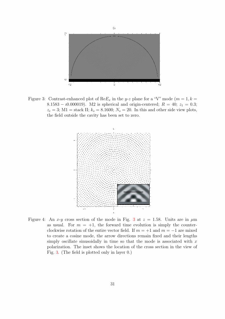
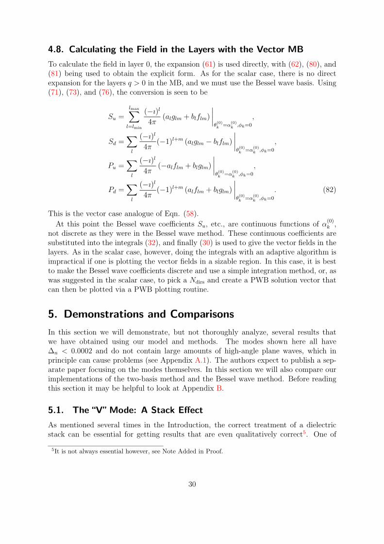
Figure 3: Contrast-enhanced plot of ReEx in the y-z plane for a “V” mode (m = 1, k =8.1583 − ı0.000019). M2 is spherical and origin-centered; R = 40; z1 = 0.3;ze = 3; M1 = stack II; ks = 8.1600; Ns = 20. In this and other side view plots,the field outside the cavity has been set to zero.
Figure 4: An x-y cross section of the mode in Fig. 3 at z = 1.58. Units are in µmas usual. For m = +1, the forward time evolution is simply the counter-clockwise rotation of the entire vector field. If m = +1 and m = −1 are mixedto create a cosine mode, the arrow directions remain fixed and their lengthssimply oscillate sinusoidally in time so that the mode is associated with xpolarization. The inset shows the location of the cross section in the view ofFig. 3. (The field is plotted only in layer 0.)
31
the most remarkable differences that we have observed when switching from simple todielectric M1 mirrors occurs right where someone looking for highly-focused, drivablemodes would be interested: the widening behavior of the fundamental Gaussian mode(the 00 mode). A Gaussian mode of a near-hemispherical cavity will become more andmore focused (wide at the curved mirror and narrow at the flat mirror) as z1 is decreased(from a starting value for which the Gaussian mode is paraxial). As the mode becomesmore focused, of course, the paraxial approximation becomes less valid and at somepoint Gaussian theory no longer applies. We have found, using realistic Al1−xGaxAs–AlAs stack models (stacks I and II described in Appendix C), that the 00 mode splitsinto two parts, so that in the side view a “V” shape is formed. Figure 3 shows a splitmode and Fig. 4 shows the physical transverse electric field, ReET ≡ ReExx + ReEyy,for this mode near the focal region. Figure 5 shows the values of Re(kR) as z1 is changedfrom 0.3 to about 0.63. Figure 6 shows a zoomed view of the field at the focus of themode at z1 = 0.63, where it is qualitatively a 00 mode. If a conducting mirror is used,the central cone simply grows wider and wider, but does not split. The V mode ispredominately s-polarized and appears in the scalar problem as well. Thus it appearsthat the V mode is a result of the non-constancy of arg(rs(α)) for a dielectric stack.We note here that following the 00 mode as z1 is changed is an imperfect process: itis possible that the following procedure may skip over narrow anticrossings that aredifficult to resolve. However, the character of the mode is maintained through suchanticrossings.
The apparent splitting of the central cone/lobe for higher order Gaussian modes hasalso been observed. In the next section we look at some higher order Gaussian modes,focusing not on what occurs at the breaking of the paraxial condition, but on what isallowed and observed for modes that are very paraxial.
5.2. Persistent Stack-Induced Mixing of Near-DegenerateLaguerre-Gaussian Mode Pairs
As mentioned in the previous section, we do observe the fundamental Gaussian modefor paraxial cavities with both dielectric and conducting planar mirrors. The situationbecomes more interesting when we look at higher order Gaussian modes. It is truethat, as modes become increasingly paraxial, Gaussian theory must apply. However,the way in which it applies allows the design of M1 to play a significant role. Herewe will demonstrate the ability of a dielectric stack (stack II) to mix near-degeneratepairs predicted by Gaussian theory into new, more complicated near-degenerate pairsof modes. We must provide considerable background to put these modes into context.Our discussion applies to modes with paraxial geometry, modes for which the paraxialparameter h ≡ λ/(πw0) = w0/zR is much less than 1. (Here w0 is the waist radius andzR is the Rayleigh range, as used in standard Gaussian theory.) In this section, thesolutions we are referring to are always the +m or −m modes discussed in Appendix B,and never mixtures of these, such as the cosine and sine modes discussed in the samesection.
32

Figure 5: Following kR as z1 is varied. The points of the two graphs correspond one-to-one, with the parameter z1 increasing from left to right in both graphs. Thepeaks in resonance width have not yet been analyzed.
5.2.1. Paraxial Theory for Vector Fields
From Gaussian theory, using the Laguerre-Gaussian (LG) basis, we expect that thetransverse electric field of any mode in the paraxial limit is expressible in the form:
ET =N∑
j=0
[A+
j
(1ı
)+ A−j
(1−ı
)]LG2j−N
min(j,N−j)(x). (83)
Here N ≥ 0 is the order of the mode. The A±j are complex coefficients and(
1ı
)and(
1−ı
)are the Jones’ vectors for right and left circular polarization, respectively. The
explicit forms of the normalized LG2j−Nmin(j,N−j) functions are given in Ref. [15] as “uLG
nm”
with the substitutions n→ N−j and m→ j. The important aspects of the LG2j−Nmin(j,N−j)
functions are that the φ-dependence is exp(ı(2j −N)φ), and the ρ-dependence includes
the factor L|2j−N |min(j,N−j)(2ρ
2/w(z)2) where Llp is a generalized Laguerre function and w(z) is
the beam radius. In the paraxial limit the vector eigenmodes of the same order become
33

Figure 6: The field in layers 0–X for the mode at z1 = 0.63. The inset shows the entiremode. The“V”nature of the mode has been lost as it has become more paraxialand more like the fundamental Gaussian. ReET everywhere lies nearly in asingle direction at any instant (here it is in the x direction). The x-z plane isshown here, although the plots of Ex in any plane containing the z axis arevery similar. Here k = 8.2098− ı0.0000401.
degenerate. There are 2(N+1) independent vector eigenmodes present in the expansion(83).
Independent from the discussion above, ET = Eρρ + Eφφ can be written as
ET =1
2(Eρ + ıEφ)︸ ︷︷ ︸∝ exp(ımφ)
eıφ( 1−ı)
+1
2(Eρ − ıEφ)︸ ︷︷ ︸∝ exp(ımφ)
e−ıφ(1ı
). (84)
Since the Eρ and Eφ fields have a sole φ-dependence of exp(ımφ), comparing with (83)reveals that, for a given m, at most two terms in (83) are present: the A−
j′+
and A+
j′−
terms where j′± = (N +m± 1)/2. Explicitly,
(Eρ ± ıEφ)/2 ≈ A∓j′±LGm±1
[N+min(m±1,−m∓1)]/2. (85)
If the solution (84) has both terms nonzero for almost all x, the constraints 0 ≤ j ≤ Nforce N to have a value given by N = |m|+1+2ν, ν = 0, 1, 2, . . . . However, if only right(left) circular polarization is present in the solution, N = |m|−1 is also allowed, providedthat m ≥ +1 (m ≤ -1). So, given a (paraxial) numerical solution with its m value, we
34

Table 1: Vector Laguerre-Gaussian modes.
can determine which orders the solutions can belong to. The reverse procedure, pickingN and determining which values of m are allowed and how many independent vectorsolutions are associated with each m, can be done by stepping j in (83) and comparingwith (84) or (85). The results for the first four orders are summarized in Table 1. TheLG0
0
(1ı
)and LG0
0
(1−ı
)modes are the fundamental Gaussian modes.
Since the cavity modes are not perfectly paraxial, the 2(N +1)-fold degenerate modesfrom the Gaussian theory are broken into N + 1 separate degenerate pairs. The trulydegenerate pairs for m 6= 0 of course consist of a +m and a −m mode which are relatedby reflection (see Appendix B). The pairings are shown in the last column of Table 1.
The dashed boxes in Table 1 enclose pairs of modes which may be mixed in a singlesolution for fixed m (Eqn. (84)). Only the mixable m = 0 modes are exactly degenerateand may be arbitrarily mixed. For the other mixable pairs, the degree of mixing willbe fixed by the cavity, in particular by the structure of M1. We now discuss our resultsregarding the mixing of the two modes with N = 2 and m = +1.
5.2.2. A demonstration of persistent mixing
Figure 7 shows the cross sections of two near-degenerate m = 1 modes found for aconducting cavity. Here z1 = ze = 0 and M2 is spherical with radius Rs = 70 but is
35

BA
Figure 7: 8 × 8 µm cross sections of modes of a conducting cavity near maximumamplitude (z = 0.25). kA = 7.89285 and kB = 7.89290. The inset plots showReEx in the x-z plane with horizontal and vertical tick marks every 1 µm.
centered at z = −59.5 instead of the origin, so that R = 10.5. The paraxial parameter his at least as small as 0.1 (see the side views in the inset plots). Mode A corresponds verywell to the pure LG0
1
(1ı
)mode, while mode B corresponds very well to the pure LG2
0
(1−ı
)mode. These are mixable modes, as indicated in Table 1, and the conducting cavity has“chosen” essentially zero mixing. Note that mode B would have zero overlap with anincident fundamental Gaussian beam centered on the z axis, while mode A would havenonzero overlap.
Pictures C and D in Figure 8 are cross sections of near-degenerate m = 1 modes for acavity with stack II. To show that the transverse part of these modes are mixtures of Aand B, we have added and subtracted the solution vectors yA and yB to create the new(non-solution) vectors:
yC′ = yA + ηyB, yD
′ = yA − (0.225)ηyB, (86)
and have plotted these fields (C′
and D′) using k = (kA + kB)/2. (The scaling factor
η, here ≈ 0.07, is unphysical and related to the effect of the seed equation on overallamplitude.) Comparing C
′and D
′with C and D shows that we have reconstructed the
mode cross sections quite well (up to a constant factor). Modes C and D are not pureHermite-Gaussian (HG) modes, but their resemblance to the HG02 and HG20 modes isnot an accident. Mode conversion formulas in Ref. [15] show that LG2
0 is made of theHG02, HG11, and HG20 modes while LG0
1 contains only HG02 and HG20. Note that bothmodes C and D would couple to a centered fundamental Gaussian beam.
An interesting property of the mixed modes C and D is that their general formsappear to be persistent as h is varied, provided that the paraxial approximation remainssufficiently applicable. Furthermore, we do not have to be particularly careful about
36
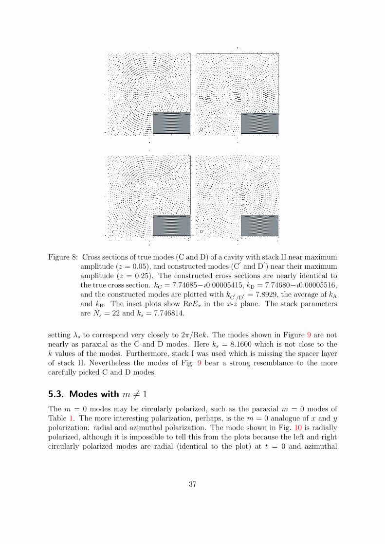
DC
C' D'
Figure 8: Cross sections of true modes (C and D) of a cavity with stack II near maximumamplitude (z = 0.05), and constructed modes (C
′and D
′) near their maximum
amplitude (z = 0.25). The constructed cross sections are nearly identical tothe true cross section. kC = 7.74685−ı0.00005415, kD = 7.74680−ı0.00005516,and the constructed modes are plotted with kC
′/D
′ = 7.8929, the average of kA
and kB. The inset plots show ReEx in the x-z plane. The stack parametersare Ns = 22 and ks = 7.746814.
setting λs to correspond very closely to 2π/Rek. The modes shown in Figure 9 are notnearly as paraxial as the C and D modes. Here ks = 8.1600 which is not close to thek values of the modes. Furthermore, stack I was used which is missing the spacer layerof stack II. Nevertheless the modes of Fig. 9 bear a strong resemblance to the morecarefully picked C and D modes.
5.3. Modes with m 6= 1
The m = 0 modes may be circularly polarized, such as the paraxial m = 0 modes ofTable 1. The more interesting polarization, perhaps, is the m = 0 analogue of x and ypolarization: radial and azimuthal polarization. The mode shown in Fig. 10 is radiallypolarized, although it is impossible to tell this from the plots because the left and rightcircularly polarized modes are radial (identical to the plot) at t = 0 and azimuthal
37

Figure 9: Cross sections of neighboring, poorly paraxial modes near maximum am-plitude (z = 1.33). M2 is spherical and origin-centered with R = 10. M1is stack I with Ns = 20, ks = 8.1600, and z1 = ze = 1.0. The modeon the left has k = 8.51160 − ı0.0002491 and the mode on the right hask = 8.51540− ı0.0003184.
(like a vortex) at ωt = π/2. The radial or azimuthal polarizations are easier to obtainnumerically than the right or left polarizations because radially (azimuthally) polarizedmodes have all of the bl (al) MB coefficients equal to zero and thus can be selected bythe seed equation (see Appendix B).
Figure 11 shows a m = 2 mode that corresponds to the LG11
(1ı
)mode from Gaussian
theory. We also have completed theN = 2 near-degenerate family by finding the LG20
(1ı
)(m = 3) mode for both the cavity used in Fig. 7 (k = 7.8926 ≈ kA ≈ kB) and the cavityused in Fig. 8 (k = 7.7466−ı0.00005466 ≈ kC ≈ kD). The cross sections of this mode forthe two cavities, which are not shown to conserve space, appear identical, as predictedby the absence of a m = +3 near-degenerate partner for this mode (Table 1).
5.4. Ndirs and lmax: Comparing the Two Primary Methods
The authors of this paper first implemented the more complicated two-basis method,believing that many more PWB coefficients than MB coefficients would be required toexpand dome-shaped cavity fields. When the Bessel wave method was implemented asa check, it was discovered that the PWB works surprisingly well, with usable valuesof Ndirs being of the same order of magnitude as usable values of lmax. The choiceof seed equation, Ndirs or lmax, and other parameters can both affect the depth andnarrowness of the dips in the graph of ∆r versus Rek. This makes it difficult to performa comprehensive and conclusive comparison of the two methods.
One practical problem with the Bessel wave method is that its performance is some-
38
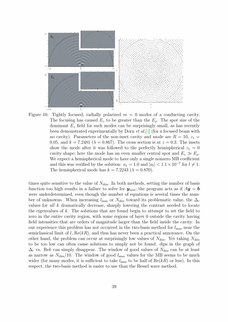
Ex
Ez
Figure 10: Tightly focused, radially polarized m = 0 modes of a conducting cavity.The focusing has caused Ez to be greater than the Eρ. The spot size of thedominant Ez field for such modes can be surprisingly small, as has recentlybeen demonstrated experimentally by Dorn et al.[4] (for a focused beam withno cavity). Parameters of the non-inset cavity and mode are R = 10, z1 =0.05, and k = 7.2481 (λ = 0.867). The cross section is at z = 0.3. The insetsshow the mode after it was followed to the perfectly hemispherical z1 = 0cavity shape; here the mode has an even smaller central spot and Ez Eρ.We expect a hemispherical mode to have only a single nonzero MB coefficientand this was verified by the solution: a1 = 1.0 and |al| < 1.1× 10⁻⁷ for l 6= 1.The hemispherical mode has k = 7.2243 (λ = 0.870).
times quite sensitive to the value of Ndirs. In both methods, setting the number of basisfunction too high results in a failure to solve for ybest; the program acts as if Ay = bwere underdetermined, even though the number of equations is several times the num-ber of unknowns. When increasing lmax or Ndirs toward its problematic value, the ∆r
values for all k dramatically decrease, sharply lowering the contrast needed to locatethe eigenvalues of k. The solutions that are found begin to attempt to set the field tozero in the entire cavity region, with some regions of layer 0 outside the cavity havingfield intensities that are orders of magnitude larger than the field inside the cavity. Inour experience this problem has not occurred in the two-basis method for lmax near thesemiclassical limit of l, Re(kR), and thus has never been a practical annoyance. On theother hand, the problem can occur at surprisingly low values of Ndirs. Yet taking Ndirs
to be too low can often cause solutions to simply not be found: dips in the graph of∆r vs. Rek can simply disappear. The window of good values of Ndirs can be at leastas narrow as Ndirs/10. The window of good lmax values for the MB seems to be muchwider (for many modes, it is sufficient to take lmax to be half of Re(kR) or less). In thisrespect, the two-basis method is easier to use than the Bessel wave method.
39

Figure 11: A m = 2 mode for a conducting cavity (k = 7.885463). M2 is spherical andorigin-centered with R = 10. M1 is a conductor; z1 = 1.0. The inset showsReEx in the x-z plane.
On the other hand, there were situations when a scan of ∆r versus Rek with theBessel wave method revealed a mode that was skipped in the same scan with the two-basis method, due to the narrowness of the dip feature. To the best of our recollection,we have always been able to find a mode by both methods if we have made an effort tosearch for it.
A direct comparison of the methods by looking at the solution plots rarely reveals fieldvalue differences greater than 1% of the maximum value when the modes are restrictedto those that do not have a large high-angle component. The eigenvalues of k locatedby the two methods are usually quite close. Here we show one case in which there is asmall but visible difference between the mode plots for the Bessel wave method and thetwo-basis method.
Figure 12 shows Ex in the x-z plane for a mode in a cavity with n0 = 1.0 and nX = 0.5and no stack layers at all. This situation is meant to model a dielectric-filled dome cavitysurrounded by air. (Our program assumes that layer 0 is free space (n0 = 1), so we haveset nX < n0 to achieve this effect.) Here M2 is spherical and centered at the origin withR = 10 and ze = z1 = 0.5. The reason for the disagreement between the two methodsfor this case is not known. This was the only low finesse cavity we have tried, as wellas being the only cavity with a “high” index of refraction in layer 0. Another unusualproperty of this mode solution, which looks similar to a fundamental Gaussian, is that its
40

Figure 12: Top: Solution obtained with Bessel wave method. k = 8.57073 − ı0.05857;∆n = 2.8 × 10⁻⁵, Ndirs = 30; α
(0)k distribution is uniform in ∆(sinα
(0)k ), not
∆(α(0)k ). Bottom: Solution obtained with two-basis method. k = 8.57086 −
ı0.05900; ∆n = 2.9× 10⁻⁵; lmax = 86. The field in layer X is not plotted.
electric field in the x-y plane actually spirals: its instantaneous linear direction rotateswith z as well as with t. The other modes we show throughout the demonstrationssection give extremely good agreement between the two primary methods.
In our implementation, computation time to set up and solve Ay = b is of the sameorder for the Bessel wave method and the two-basis method (with variant 1). For thelarge cavity shown in Fig. 3, the Bessel wave method took about 10 s with Ndirs = 100and about 600 locations chosen on M2. Variant 1 with lmax = 200, 600 M2 locations,and 600 uniformly spaced α
(0)k , took about 15 s. For comparison, Variant 2 took about
2 hours (achieving a 10−6 relative accuracy for each α(0)k integral).
5.5. Almost-Real MB Coefficients
When M1 is a conductor we find that the imaginary parts of al and bl are essentially zero.Furthermore, we often find that for dielectric M1 mirrors, the imaginary parts of al andbl are one or more orders of magnitude smaller than their real parts. We show one wayin which this tendency simplifies the interpretation of mode polarization in Appendix B.
There is a an argument that suggests that al and bl should be real for a conductingcavity. A conducting cavity has a real eigenvalues, k, and real reflection functions,
41

rs/p = −1. It is not difficult to see that for real k the three types of M2 equations,Eφ = 0, E‖ = 0, and H⊥ = 0, can be satisfied with real al and bl. The seed equation ofcourse can also be chosen so that it can be satisfied by real variables. The M1 equations,because of the complex nature of rs/p = rs/p exp(−ı2z1kn0 cosα
(0)k ) when z1 6= 0, are not
obviously satisfied by real al and bl. However, for a conducting cavity, the M1 boundarycondition can be given as a real space boundary condition (like M2) instead of a Fourierspace boundary condition. In this case, locations on M1 are chosen just as they are onM2. The same argument that the M2 equations can be satisfied by real al and bl nowapplies. Thus the M1 boundary condition for a conducting cavity should not, in anybasis, force al and bl to be complex.
6. Conclusions
The two methods presented in this communication have proved to be useful tools formodeling small optical dome-shaped cavities. As yet we have no general verdict on whichmethod is best. Overall, it was quite helpful to have both methods available for findingall of the modes. Once a mode was found, agreement of both eigenvalue and eigenmodebetween the two methods was quite good.
The primary advantage of both of these methods is the treatment of the dielectricstack through its transfer matrices. First of all, including the dielectric stack in themodel is essential to obtain a number of qualitative features of the modes. A modelwith a mirror of constant phase shift is inadequate, except in special cases such as thefundamental Gaussian mode in its paraxial regime. In addition, including the stack inthe model allows one to calculate the field inside the stack, which may be the location ofinterest for the engineer of an optical device. Secondly, the use of the transfer matrices isthe most natural way to include a dielectric stack that is of large lateral extent comparedto the wavelength. The only alternative that we know of would involve a separate basisfor each stack layer, resulting in an increase of both dimensions of the matrix A by aboutN times, where N is the number of stack layers.
Another advantage of the methods we have presented is their speed. Each point inFig. 5, which was generated in a few hours or less, required Ay = b to be constructedand solved 20–60 times for a cavity with R ≈ 50λ. The combination of using a basisexpansion method, taking advantage of cylindrical symmetry, using one basis set for allthe layers, avoiding numerical integrals, and using C++ inline functions for complexarithmetic has resulted in a fast implementation.
Several“stack-induced”effects that we have demonstrated here will be more thoroughlytreated in a separate publication. The splitting of the fundamental Gaussian (and otherGaussian modes) into a non-axisymmetric “V” shape may be of practical interest toworkers who wish to achieve a tight focus. The m = 0 modes, which have the greatestpotential for tight focusing, are also of interest. The ability to analyze the persistentstack-induced mixing is a result that stands in its own right. This stack effect persistsarbitrarily far into the paraxial limit; it exists as long as the resonance widths of boththe cavity and the laser source are smaller than the splitting of the near-degenerate pair.
42

This effect should exist for a wide range of cavity lengths, and is of interest to anyoneengineering higher-order Gaussian modes.
Perhaps the greatest limitation to the practical application of our methods is its rigidtreatment of the curved mirror as a conductor. As mentioned in the Introduction, it isreasonable to expect highly focused modes, such as those shown in Figs. 3, 6 and 10, toundergo little change when the curved conducting mirror is exchanged for a dielectricone (with an appropriate change of mirror radius by −λ/4 < δ < λ/4 to account for aphase shift). This is because the local wave fronts are primarily perpendicular to thecurved mirror for such modes (imagine a Wigner function evaluated at the surface ofM2). For paraxial geometries such as those in our discussion of stack-induced mixing,this argument says nothing about how replacing M2 with a curved dielectric stack willaffect the modes. A pursuit of this question may require a more brute force approach.
Despite all limitations, we find our methods to be extremely versatile and powerful(fast and allowing for relatively large cavities). The full vector electromagnetic field isused. Exactly degenerate modes can be separated. The shape of the curved mirror isarbitrary and we have implemented parabolic shapes as well as spherical shapes with nodifficulties. A first-try scan of ∆r versus Rek using either method with a non-contrivedseed equation will locate the vast majority of modes that exist. Reasonable results areobtained when the interior of the cavity is a dielectric. Hopefully, the explicit develop-ment of the two methods given here can benefit a number of workers in optics-relatedfields.
Note Added in Proof
We note that we have not found significant stack-induced effects (the V mode of Section5.1 and the mixing of Section 5.2) for a“standard”quarter-wave dielectric stack which hasdesign ABAB. . .AB with front surface A and nA > nB. If nA < nB, we do find both typesof stack-induced effects. The standard (nA > nB) quarter-wave layer structure exhibitsless variation in arg(rs/p(αk)) than our mirrors (cf. Fig. 15), and therefore behaves muchlike a perfect conductor except at high angles of incidence. The methods presented here,which model the curved dome mirror (M2) as a conductor, should therefore carry overto standard dielectric M2 mirrors. The planar mirror will in general have a “functional”layer design, leading to the stack-induced effects reported above.
Acknowledgments
We would like to thank Prof. Michael Raymer for getting us interested in the realisticcavity problem. This work is supported by the National Science Foundation throughCAREER Award No. 0239332.
43

A. Further Explanations and Limitations of the Model
A.1. Exclusion of High-Angle Plane Waves
As mentioned in the Introduction, in the usual application of a basis expansion method,the field is expanded in each dielectric region separately and henceforth each region getsits own complete basis and its own set of coefficients. However, our methods, when“cast”into the PWB, use a single set of plane waves, complete in layer 0, which are propagateddown into the other layers via the transfer matrices. There are several advantages to thisapproach. The Bessel wave method becomes simpler, as there are far fewer unknowns.This approach is also ideal for incorporating the use of the MB for layer 0, as in thetwo-basis method, although a straightforward use of the MB for layer 0 and a separatePWB for each layer q, q > 0, could be implemented.
One drawback to our approach is that certain high-angle or evanescent plane wavesare not included. No plane wave basis vectors are allowed for which nq sin θ
(q)k > n0. If
the true quasimode expansion in any layer has significant weight for these high-angle orevanescent waves, the calculated solution of the field could be erroneous.
Probably the best way to determine whether or not such intrinsic error is present ata significant level is to look at the plane wave distribution in layer 0 (using (58) or (82)to get this if one is using the two-basis method) and to see whether the distribution dies
off as α(0)k approaches π/2. If it does, the solution should be reasonably error free.
We note here that Berry [16] has shown how evanescent waves, in a finite region nearthe origin, can be expressed in the PWB (using plane waves with real-valued directions,as usual). Thus the fact that no evanescent waves are included in layer 0 may not be aproblem in itself for depicting the field in layer 0.
A.2. The Hat Brim
A.2.1. The infinitesimal hat brim
Figure 13: Modeling the edge of the dome.
For the vector field solution, a tiny hat brim must be added to M2 to correctly modela conducting edge. Figure 13 shows a cross section of the edge of M2 for increasingly
44

better approximations of a real conducting mirror. In (a), Eρ can be nonzero at theedge, which is unphysical. In (b), a small hat brim has been added and E = 0 at theinside edge, as it should be. In (c), locations are chosen on a (closed) conductor withfinite thickness. As the thickness of M2 becomes insignificant compared to λ, model (b)should approximate model (c) arbitrarily closely. Usually 2–10 locations are chosen onthe hat brim (the density of course is much greater on the hat brim than on the dome).We have taken ωb ≈ 0.0001µm for our demonstrations.
A.2.2. The infinite hat brim and the 1-D half-plane cavity
The way in which our model includes the interior of the cavity and the entire z > z1
half-plane in a single region, layer 0, is somewhat unorthodox. We believe our methodproduces the correct field in a finite region surrounding the cavity, but not at z →∞.
A somewhat less strange model is obtained if one imagines an infinite hat brim. Theupper half-plane is then no longer in the problem. Layer 0 still extends infinitely in ρas do the other layers, but the vertical confinement makes it easier to see that this isan eigenproblem and not a scattering problem. Unfortunately our implementation doesnot allow an infinite hat brim (unless M1 is a conductor and ze = z1, for which the hatbrim condition is already set in the M1 equations). At least for some solutions, takingwb ≈ R and giving the hat brim roughly the same number of locations as the dome,produces no visible changes in the mode structure (from the solution obtained with atiny hat brim). The mode shown in Fig. 3 is one of these.
Figure 14: Including the sides of the stack at radius ρfinite.
If we allow that some solutions are not affected by the value of wb, we can take theinfinite hat brim more seriously. The problem becomes similar in some respects to the1-D half-plane problem, in which x < 0 is a conductor, x > L has a constant refractiveindex, and the [0, L] region is segmented into several 1-D dielectric layers. The solutionsof the 1-D problem form a set of quasimodes, (or quasinormal modes), which are complete
45
in [0, L] and obey an orthogonality condition on the same interval. The conditions forcompleteness, and the characterization of the incompleteness of the quasinormal modefor problems which do not meet the completeness conditions, are discussed in Ching etal. [17] and Leung et al. [18]. The model with the infinite hat brim does not rigorouslymeet the the completeness condition (for 3-D cavity resonators). We note that it appearsfrom the references mentioned above that the situation depicted in Fig. 14 would meetthe completeness condition, with the quasinormal modes being complete in layers 0–N .We do not attempt to resolve this further, as the use of our mode solutions as a basis fortime-dependent problems is beyond the scope of what we have been trying to accomplish.
B. Negative m Modes and Sine and Cosine Modes
The cylindrical symmetry group consists of φ-rotations and reflections about the x-z ory-z planes. For solutions with a fixed, nonzero m, rotations are equivalent to multiplyingthe field by a complex phase, which is of course equivalent to a translation in time. (Thismeans that, when looking at any cross section plot in Section 5 for a fixedm 6= 0, the timeevolution can be realized by simply rotating the figure: counter-clockwise for m > 0 andclockwise form < 0.) Thus we say that form 6= 0, reflections generate a new solution butrotations do not. (If we were considering the sine and cosine modes discussed later in thesection, instead of the ±m modes, we would say that a π/(2m) rotation generates a newsolution but a reflection does not.) Hence the symmetry of the cavity causes modes tocome in truly degenerate pairs. It can be shown that a reflection is equivalent to takingm to −m (up to a π rotation). For m 6= 0, general complex linear superpositions of the±m pair of modes are equivalent to arbitrary complex superpositions of any number ofφ-rotations, reflections, and combinations of these acting on a single +m mode. We notethat since our methods solve y for a fixed m, we are able to separate the ±m pairs.
The m = 0 modes also come in degenerate pairs, but the interrelation can be morecomplicated than a reflection. The m = 0 pairs can be separated easily in the two-basismethod by choosing a seed equation that contains only al or only bl coefficients, sincethe M1 and M2 equations do not couple al and bl coefficients if m = 0. Thus all of thetrue (non-accidental), exact (not obtained only in a limit, such as the paraxial limit)degeneracies that exist can be separated.
In constructing the M1 and M2 equations, it is easiest to write code that assumes thatm ≥ 0. For presentations and movies, it is nice to be able to plot both +m and −msolutions, as well as the linear combinations adding and subtracting these modes. Allfour of these modes can be plotted from a solution y+m that has been been found usingthe positive azimuthal quantum number +m. Here we briefly discuss how to do this (form 6= 0).
B.1. Plotting with -m
To plot the −m modes, we use simple rules, allowed by the M1 and M2 equations, tocreate a new solution vector y−m from the solution y+m. To obtain the field, the new
46

coefficients from y−m are simply inserted into the various expansion (or basis conversion)equations from Sections 3 and 4, using (−m) as the “m” argument in these equations.(All of these equations work for negative values of their m argument.) The relationsYl,−m = (−1)mY ∗
lm, J−m = (−1)mJm, fl,−m = (−1)mflm, and gl,−m = −(−1)mglm areuseful. The rules for the new solution vectors are given in Table 2. (There is a certainarbitrariness to these rules, since (αy), with α being an arbitrary constant, satisfies theM1 and M2 equations.)
Table 2: Rules for taking y+m → y−m.PWB MB
scalar: ψu,−m = (−1)mψu,+m cl,−m = cl,+m
vector: Su/d,−m = −(−1)mSu/d,+m al,−m = al,+m
Pu/d,−m = (−1)mPu/d,+m bl,−m = −bl,+m
B.2. Plotting cosine and sine modes
We can define the “cosine” and “sine” modes as X(c) ≡ (X(+m) + (−1)mX(−m))/2, andX(s) ≡ (X(+m) − (−1)mX(−m))/2, where X stands for ψ, E, or H . By adding explicitexpansion expressions for the +m and −m modes, one can obtain expressions for X(c)
and X(s). For example, using (61), (62), and the above rules one finds that
E(0)(c) (x, t) = e−ıωt
∑l
r
[al−l(l + 1)
kn0rjlReYlm
]+ θ
[al−1
kn0r
∂
∂r(rjl)
∂
∂θ(ReYlm) + bl
−msin θ
jlReYlm
]+ φ
[al
m
kn0r sin θ
∂
∂r(rjl)ImYlm + bljl
∂
∂θ(ImYlm)
],
where al and bl come from the original y+m. When al and bl are predominately real(see Section 5.5), we can see from the above equation that the real-valued physical fieldsEρ and Ez are proportional to cosmφ cosωt while Eφ is proportional to sinmφ cosωt.(The cosine time-dependence of E is why we call this the cosine mode.) Thus for thecosine mode with |m| = 1, the transverse portion of E has an average linear polarizationalong the x axis (note 〈Ey〉φ = 0 ∀t), as opposed to the average circular polarizationthe m = ±1 modes would have. (For the m = +1 mode, 〈E · q〉φ = 0 ∀t whereq ≡ −x sinωt + y cosωt.) Due to their separating of time and φ-dependence for thephysical fields, the sine and cosine modes are very useful final forms of the field (whenal and bl are predominately real).
47
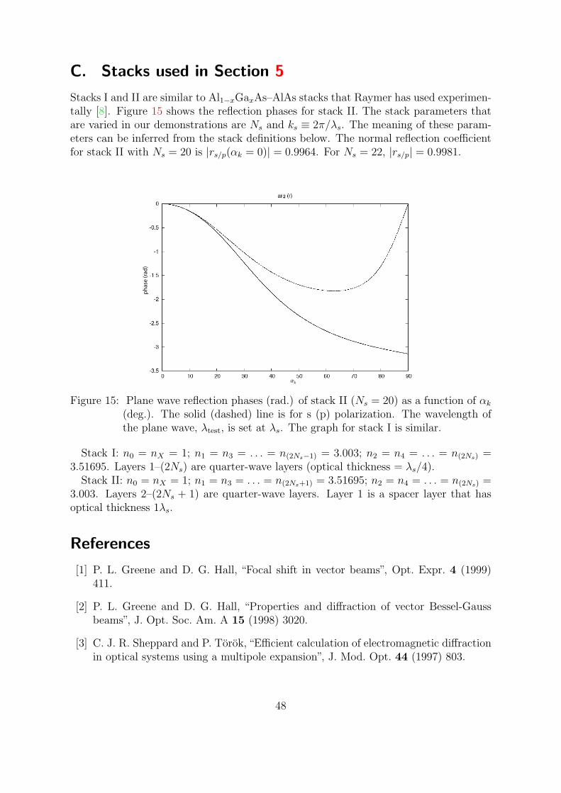
C. Stacks used in Section 5
Stacks I and II are similar to Al1−xGaxAs–AlAs stacks that Raymer has used experimen-tally [8]. Figure 15 shows the reflection phases for stack II. The stack parameters thatare varied in our demonstrations are Ns and ks ≡ 2π/λs. The meaning of these param-eters can be inferred from the stack definitions below. The normal reflection coefficientfor stack II with Ns = 20 is |rs/p(αk = 0)| = 0.9964. For Ns = 22, |rs/p| = 0.9981.
ph
ase
(rad
)
Figure 15: Plane wave reflection phases (rad.) of stack II (Ns = 20) as a function of αk
(deg.). The solid (dashed) line is for s (p) polarization. The wavelength ofthe plane wave, λtest, is set at λs. The graph for stack I is similar.
Stack I: n0 = nX = 1; n1 = n3 = . . . = n(2Ns−1) = 3.003; n2 = n4 = . . . = n(2Ns) =3.51695. Layers 1–(2Ns) are quarter-wave layers (optical thickness = λs/4).
Stack II: n0 = nX = 1; n1 = n3 = . . . = n(2Ns+1) = 3.51695; n2 = n4 = . . . = n(2Ns) =3.003. Layers 2–(2Ns + 1) are quarter-wave layers. Layer 1 is a spacer layer that hasoptical thickness 1λs.
References
[1] P. L. Greene and D. G. Hall, “Focal shift in vector beams”, Opt. Expr. 4 (1999)411.
[2] P. L. Greene and D. G. Hall, “Properties and diffraction of vector Bessel-Gaussbeams”, J. Opt. Soc. Am. A 15 (1998) 3020.
[3] C. J. R. Sheppard and P. Torok, “Efficient calculation of electromagnetic diffractionin optical systems using a multipole expansion”, J. Mod. Opt. 44 (1997) 803.
48

[4] R. Dorn, S. Quabis, and G. Leuchs, “Smaller, sharper focus for a radially polarizedlight beam”, Phys. Rev. Lett. 91 (2003) 233901.
[5] J. U. Nockel, G. Bourdon, E. Le Ru, R. Adams, I. Robert, J-M. Moison, I. Abram,“Mode structure and ray dynamics of a parabolic dome microcavity”, Phys. Rev. E62 (2000) 8677.
[6] J.U. Nockel and R.K. Chang, ”2-d Microcavities: Theory and Experiments”, inCavity-Enhanced Spectroscopies, Roger D. van Zee and John P. Looney, eds. (Exper-imental Methods in the Physical Sciences 40), Academic Press, San Diego (2002),185–226.
[7] A. E. Siegman, Lasers, University Science Books, Sausalito, CA, 1986, pp. 626–97,744–76.
[8] M. G. Raymer (colloquium, University of Oregon, 4/24/03, and private communi-cation).
[9] M. Aziz, J. Pfeiffer, and P. Meissner, “Modal Behaviour of Passive, Stable Micro-cavities”, Phys. Stat. Sol. (a) 188 (2001) 979.
[10] J. D. Jackson, Classical Electrodynamics, Third Edition, John Wiley & Sons, Inc.,New York, 1999, pp. 107–10, 113–4, 426–32, 471–73.
[11] P. Yeh, Optical waves in layered media, Wiley, New York, 1988, pp. 60–64, 102–15.
[12] W. H. Press, S. A. Teukolsky, W. T. Vetterling, B. P. Flannery, Numerical Recipesin C: The Art of Scientific Computing, Second Edition, Cambridge University Press,Cambridge, 1992, pp. 59–70, 359–62.
[13] G. B. Arfken and H. J. Weber, Mathematical Methods for Physicists, Fifth Edition,Harcourt Academic Press, San Diego, 2001, p. 767.
[14] G. Videen, “Light Scattering from a particle on or near a perfectly conductingsurface”, Optics Communications 115 (1995) 1.
[15] M. W. Beijersbergen, L. Allen, H. E. L. O. van der Veen, and J. P. Woerdman,”Astigmatic laser mode converters and transfer of orbital angular momentum”. Op-tics Communications 96 (1993) 123.
[16] M. V. Berry, “Evanescent and real waves in quantum billiards and Gaussian beams”,J. Phys. A: Math. Gen. 27 (1994) L391.
[17] E. S. Ching, P. T. Leung, A. Maassen van den Brink, W. M. Suen, S. S. Tong, K.Young, “Quasinormal-mode expansion for waves in open systems”, Rev. Mod. Phys.70 (1998) 1545.
[18] P. T. Leung, S. Y. Liu, and K. Young, “Completeness and orthogonality of quasi-normal modes in leaky optical cavities”, Phys. Rev. A 49 (1994) 3057.
49