1

METHODOLOGY FOR ESTIMATING SEISMIC COEFFICIENTS FOR

PERFORMANCE-BASED DESIGN OF EARTHDAMS AND TALL

EMBANKMENTS

Achilleas G. Papadimitriou

Assistant Professor, Department of Civil Engineering,

University of Thessaly, Greece

George D. Bouckovalas

Professor, Geotechnical Department, School of Civil Engineering,

National Technical University of Athens, Greece

Konstantinos I. Andrianopoulos

Post-Doctoral Researcher, Geotechnical Department, School of Civil Engineering,

National Technical University of Athens, Greece

Paper submitted for publication to Soil Dynamics and Earthquake Engineering

Text + 1 Table & 15 Figures

KEYWORDS: earthdams, earthquake, embankments, non-linear soil response,

numerical analysis, performance-based design, pseudo-static analysis,

sliding block, slope stability

CONTACT ADDRESS: Achilleas Papadimitriou Department of Civil Engineering University of Thessaly Pedion Areos, 38334, Volos, Greece Tel. +30-24210-74140 Fax. +30-24210-74169 Email. apapad@civ.uth.gr Web. http://apapad.users.uth.gr

2

METHODOLOGY FOR ESTIMATING SEISMIC COEFFICIENTS FOR

PERFORMANCE-BASED DESIGN OF EARTHDAMS AND TALL

EMBANKMENTS

Achilleas G. Papadimitriou1, George D. Bouckovalas2

Konstantinos I. Andrianopoulos3

Abstract

Following an overview of pertinent literature, this paper presents a new methodology for

estimating seismic coefficients for the performance-based design of earth dams and tall

embankments. The methodology is based on statistical regression of (decoupled) numerical

data for 1084 potential sliding masses, originating from 110 non-linear seismic response

analyses of 2D cross sections with height ranging from 20 to 120m. At first, the methodology

estimates the peak value of the seismic coefficient khmax as a function of: the peak ground

acceleration at the free field, the predominant period of the seismic excitation, the non-linear

fundamental period of dam vibration, the stiffness of the firm foundation soil or rock layer, as

well as the geometrical characteristics and the location (upstream or downstream) of the

potentially sliding mass. Then, it proceeds to the estimation of an effective value of the

seismic coefficient khE, as a percentile of khmax, to be used with a requirement for pseudo-

static factor of safety greater or equal to 1.0. The estimation of khE is based on allowable

permanent down-slope deviatoric displacement and a conservative consideration of sliding

block analysis.

Keywords— earthdams, earthquake, embankments, non-linear soil response, numerical analysis, performance-based design, pseudo-static analysis, sliding block, slope stability

1 Assistant Professor, Department of Civil Engineering, University of Thessaly, Greece, < apapad@civ.uth.gr > 2 Professor, Department of Geotechnical Engineering, School of Civil Engineering, National Technical

University of Athens, Greece, < gbouck@central.ntua.gr > 3 Post-Doctoral Researcher, Department of Geotechnical Engineering, School of Civil Engineering, National

Technical University of Athens, Greece, < kandrian@tee.gr >

3

1. INTRODUCTION

It is well known that the assessment of seismic stability of earth structures may be performed

via: (a) traditional and easy to use pseudo-static analyses, (b) a great number of available

displacement-based (Newmark or sliding block) methods, and (c) dynamic stress-deformation

numerical analyses. Although robust numerical analyses, i.e. method (c), are nowadays quite

common, methods (a) and (b) are still the basis of engineering practice in the aseismic design

of earth dams and natural slopes worldwide, at least in the preliminary design stages.

Pseudo-static analyses have the benefit of accumulated experience, reduced cost and user-

friendliness, since they merely require the estimation of a Factor of Safety FSd against

seismic “failure” of the slopes of the earth structure. The described problem is illustrated in

Fig. 1, which also depicts significant problem parameters like the peak values of the seismic

acceleration at the crest, PGAcrest, at the outcropping (bed)rock PGArock and at the “free-field”

of the foundation soil, PGA. The critical measure of the whole analysis is the value of the

horizontal inertial force Fh that is applied at the center of gravity of the sliding mass and

equals to the weight of the mass W multiplied by a dimensionless seismic coefficient kh. At

any rate, the value of Fh (and kh) should reflect the vibration of the sliding mass during the

design earthquake, and its rational selection is therefore critical.

Given that the sliding mass is not rigid, different locations within this mass do not vibrate in

phase and with the same intensity. For instance, this is especially true for deep sliding masses

in tall dams where vibration is less intense deep within the dam body, as compared to its

surface, and the predominant wave length λd of the seismic shear waves within the dam body

is comparable to the dam height H. Therefore, the value of kh should be related to the

resultant (horizontal) acceleration time history of the sliding mass, which, in turn, has been

related to the resultant (horizontal) force time history along the shear band delineating the

sliding mass within the dam body. This resultant acceleration time history is generally not

4

equal to the acceleration time history at any standard “reference” location within, or in the

vicinity of the dam (e.g. the “free-field” of the foundation soil, the outcropping bedrock, the

crest of the dam or its base). On the contrary, this resultant acceleration time history is

generally expected to be a function of the characteristics of the dam and the excitation, as

well as the geometry of the sliding mass (Makdisi and Seed 1978), but also to be affected by

whether slippage has initiated along the shear band that delineates the sliding mass within the

dam body (Rathje and Bray 2000).

Overall, there are two types of numerical procedures for estimating resultant acceleration

time histories (and displacements) of sliding masses, i.e. “decoupled” procedures where the

dynamic response of the examined dam is calculated separately from possible slippage of any

sliding mass within it (e.g. Makdisi and Seed 1978, Lin and Whitman 1983) and “coupled”

procedures where the dynamic response of the sliding mass (and not the dam) is considered

simultaneously to the accumulation of permanent deviatoric displacement (e.g. Kramer and

Smith 1997, Rathje and Bray 2000). In any case, it becomes obvious that an accurate

estimation of the resultant time history of a flexible sliding mass requires robust dynamic

numerical analyses, which are demanding in software, expertise and cost, and hence beat the

purpose of choosing method (a) over (c). Hence, in order to avoid such analyses, researchers

and practitioners around the world have devised various empirical methods for estimating

appropriate values of seismic coefficients to be used in pseudo-static analyses (e.g. USCOLD

1985, Charles et al. 1991). Andrianopoulos et al. (2012) presents a critical evaluation of such

methods and shows that they generally disregard important problem parameters (e.g. dam

characteristics) and may prove unconservative (e.g. for shallow sliding masses).

Yet, in all cases, the peak of the resultant acceleration time history, denoted hereafter as khmax,

has never been considered an appropriate value of kh for use in pseudo-static analyses. This is

because khmax is observed momentarily and therefore an analysis using this value along with a

5

requirement for FSd ≥ 1.0 leads to an over-conservative design. Hence, common practice

dictates the use of an “effective” value of the seismic coefficient khE (a percentile of khmax) in

combination with the requirement for FSd ≥ 1.0, as more representative of the overall

intensity of the shaking throughout its duration. This khE/khmax ratio in the literature ranges

from 0.5 to 0.8, and its value has mostly been selected on the basis of experience and

intuition (Papadimitriou et al. 2010). This simple method of rationalizing the design comes at

the expense of generally “small”, but yet unknown, permanent down-slope deviatoric

displacements (e.g. Hynes-Griffin and Franklin (1984) suggest that use of khE/khmax = 0.5

leads to displacements less than 30cm, a value corroborated by Bozbey and Gundoglu (2011)

who also showed that for PGA less than 0.5g these displacements are even less than 20cm).

Based on the above, it becomes obvious that permanent down-slope deviatoric displacements

don’t directly govern, but are related to the selection of an “effective” seismic coefficient for

the traditional pseudo-static design of earth dams and tall embankments, or method (a) above.

On the contrary, nowadays, these displacements play the lead role in modern performance-

based design of such structures, or method (b) above. In particular, Newmark (1965), being

the pioneer of this effort, devised the rigid sliding block theory for downslope deviatoric

displacement computations based on the estimation of the yield acceleration of the sliding

mass kyg (where g is the acceleration of gravity and ky the yield seismic coefficient), via trial-

and-error pseudo-static analyses for FSd = 1. Note that this threshold value of (yield)

acceleration indirectly reflects the strength of the geomaterials along the shear band and the

geometry and weight of the sliding mass. According to this method, the accumulated

downslope deviatoric displacements of the slopes may be obtained by double integration of

the relative acceleration, i.e. of the difference between the resultant acceleration time history

and the critical acceleration kyg of the sliding mass

In Newmark’s proposition, the sliding mass was considered rigid and required case-specific

6

time-histories for estimating displacements. To alleviate the latter problem, many research

efforts ever since have made parametric use of this basic concept for a large number of

seismic recordings attempting to devise user-friendly equations and/or charts for estimating

permanent down-slope displacements, given different selections of seismic motion measures

(e.g. earthquake magnitude M, PGA, peak ground velocity PGV, Arias intensity,

predominant Te excitation period) and the value of the yield seismic coefficient ky (e.g.

Franklin and Chang 1977, Richards and Elms 1979, Whitman and Liao 1984, Ambraseys and

Menu 1988, Cai and Bathurst 1996, Jibson 2007, Saygili and Rathje 2008, Bozbey and

Gundoglu 2011). Realizing further that the rigid block assumption is potentially too crude for

a deep and flexible sliding mass, many researchers went on to estimate the resultant

acceleration time-history and the down-slope displacement of this sliding mass, either with

“decoupled” (e.g. Makdisi and Seed 1978) or with “coupled” analyses (e.g. Rathje and Bray

2000). Again, parametric analyses for large databases of seismic recordings enabled the

proposal of empirical equations and/or design charts for estimating permanent down-slope

displacements using “decoupled” (e.g. Makdisi and Seed 1978, Bray and Rathje 1998), but

mostly “coupled” analyses (e.g. Bray and Travasarou 2007, Rathje and Antonakos 2011). The

proposed equations and/or design charts appropriately employed seismic intensity measures

related to the resultant acceleration time history of the sliding mass (e.g. khmax), rather than

the seismic excitation itself (e.g. PGA) as in rigid sliding block methods. Hence, besides the

need for estimating ky via pseudo-static analyses, some of these displacement-based methods

also include procedures for estimating the peak seismic coefficient, khmax. Again,

Andrianopoulos et al. (2012) performs a critical evaluation of such procedures, and shows

that they may also disregard important problem parameters (e.g. reservoir impoundment,

existence of berms), while, in some cases, they are cumbersome to employ since they are not

stand-alone methodologies (e.g. Makdisi and Seed 1978 require the independent estimation

7

of PGAcrest).

In conclusion, methods (a) and (b) for the seismic design of earth dams and tall embankments

are, in reality, clearly interrelated. Acknowledging this fact, there are efforts in the literature

lately to directly relate the appropriate selection of an “effective” seismic coefficient khE (for

use in pseudo-static analyses) to the allowable downslope deviatoric displacement (Biondi et

al. 2007, Bray and Travasarou 2009, Zania et al. 2011, Bozbey and Gundogdu 2011). These

efforts definitely reduce the arbitrary nature by which the khE/kmax ratio has been dealt with in

the past. Yet, Biondi et al (2007) and Bozbey and Gundogdu (2011) deal with very specific

sliding mass geometries (infinite slope, wedge in slope) that cannot cover all potential sliding

masses of earthdams and tall embankments. On the other hand, Bray and Travasarou (2009)

propose an elegant scheme for estimating khE by considering it equal to ky and requiring that

FSd = 1 for a given level of allowable displacements. To do so they propose an equation that

uses an intensity parameter that is not yet well-established in engineering practice (spectral

acceleration Sa for an elongated period of the sliding mass) and is related to the seismic

excitation and not the dam vibration. Finally, Zania et al (2011) propose a “seismic coefficient

spectrum” that yields values of khE < khmax as a function of slope displacements. In concept, it

is a rational approach, since it incorporates resonance and out-of-phase dam vibration effects,

but their results pertain to specific sliding mass geometries and come with significant scatter

due to the employed correlation to PGA, rather than PGAcrest (the latter is related to dam

vibration, but not the former).

This paper falls within this last category of recent research efforts and aims at explicitly

introducing performance-based design concepts in the well-known (to practitioners)

methodology of pseudo-static analysis. It also aims to propose a stand-alone and easy-to-use

method for any potential sliding mass geometry, and to take into account all important

problem parameters, thus remedying the insufficiencies of existing methodologies from the

8

literature. To do so, it first proposes a methodology for independent estimation of the peak

seismic coefficient khmax (Section 3) and then proceeds to the estimation of its “effective”

value khE based on allowable displacements and a conservative consideration of sliding block

analysis (Section 4). These tasks are enabled by statistical regression of numerical results

originating from a large number of two dimensional (2D) non-linear seismic response

“decoupled” analyses of earth dams (for actual acceleration time histories), which address

parametrically the effects of all important problem parameters (Section 2). The paper ends

(Section 5) with a discussion on the accuracy and the limitations of the proposed

methodology.

2. DESCRIPTION OF NUMERICAL ANALYSES

2.1 Overview

Attempting a “decoupled” approach to the problem, the numerical investigation is based on a

total of 110 two-dimensional (2D) seismic response analyses of earthdams that yielded results

for 1084 potential sliding masses. These non-linear analyses were executed using the

commercial finite difference code FLAC (Itasca, 2005), that performs integration of wave

equations in the time domain. The analyses studied parametrically the effects of:

− Intensity and frequency content of the excitation (PGA = 0.05 - 0.5g, Te = 0.14 – 0.5s)

− Foundation conditions (shear wave velocities of the foundation soil, Vb = 250 – 1500m/s)

− Existence of (large) stabilizing berms

− Reservoir impoundment, and

− The exact geometry of the potential sliding mass

9

As described in Andrianopoulos et al. (2012), most of these parameters are not accounted for

in existing methodologies for estimating seismic coefficients for earthdams and tall

embankments. Hence, the study here focused on the effects of the foregoing parameters on

three (3) fundamental aspects of seismic response of such geostructures, namely the non-

linear fundamental period of dam vibration, To, the peak acceleration at the dam crest,

PGAcrest, and the peak value of the seismic coefficient khmax for various sliding masses within

the dam body.

In order to provide for the greatest possible applicability of the methodology, the response of

four (4) cross sections was analyzed parametrically, namely cross sections of:

− H = 20m (tall embankment, with base width equal to 80m)

− Η = 40m (rather short earth dam, with base width equal to 210m)

− Η = 80m (medium height earth dam, with base width equal to 415m)

− Η = 120m (tall earth dam, with base width equal to 615m)

The slope inclinations of the earth dams ranged from 1:2 to 1:2.5 (vertical : horizontal) in

order to ensure ample static stability. In the cases of H = 40, 80 and 120m the earth dam

possessed a clay core with slope inclinations ranging from 4:1 to 5:1, while for the case of H

= 20m the embankment was considered uniform.

In order to investigate the effect of stabilizing berms on the seismic response of an earthdam,

variations of the foregoing sections were also studied. These variants of dam sections

possessed typical berms of height and width equal to Η/3 and 2Η/3 respectively on both sides

of the body of the dam, for H = 40 and 80m. Furthermore, in order to investigate the effect of

foundation conditions on the seismic response, the same cross sections of dams were

analyzed for various shear wave velocities of the foundation soil, from Vb = 250m/s up to

1500m/s (the smaller value only for H=20m). Finally, in order to investigate the effect of

10

reservoir impoundment on the seismic response, the same cross sections were analyzed for

end of construction and steady state seepage conditions. The former conditions pertain to

unsaturated geomaterials comprising the dam, while the latter to saturated upstream

geomaterials and a fully impounded reservoir.

The finite difference analyses were performed with dense meshes (maximum zone dimension

equal to 1/10 of the predominant shear wavelength) of large dimensions (e.g. lateral extent of

at least 2H), that were equipped with proper boundary conditions (e.g. free-field lateral

boundaries). The employed seismic excitations were based on recordings from actual

earthquakes, with the predominant periods Te ranging between 0.14sec and 0.50sec, i.e.

covering the whole range of usually expected (at least in Southern Europe) significant periods

for bedrock excitations. Further details on the numerical simulations and their results may be

found in Bouckovalas et al (2009) and Andrianopoulos et al (2012).

2.2 Constitutive model for geomaterials

The mechanical response under dynamic loading of the various geomaterials comprising the

earthdams was simulated via the non-linear hysteretic constitutive model described below,

that has been implemented as a User-Defined-Model routine by the authors. In all cases, the

soil is modeled as a non-linear hysteretic material using constantly updating values of the

tangential bulk Kt and shear Gt moduli. In particular, following isotropic elasticity, the Kt and

Gt are interrelated via a constant elastic Poisson’s ratio ν (a model constant). Then, based on

Andrianopoulos et al (2010), Andrianopoulos (2006) and Papadimitriou (1999), the non-

linear hysteretic form of Gt is given the following generalized Ramberg and Osgood (1943)

type of relation for monotonic and cyclic loading paths:

T

GG max

t = (1)

11

1 1

1 1

1 X1 2 1 , for cyclic loading

a 2ηT 1

1 X1 2 1 , for monotonic loading

a η

+ −

= ≥

+ −

(2)

where Gmax is the maximum (small-strain) shear modulus and T is a dimensionless scalar that

varies during loading introducing Gt degradation (and as an effect hysteretic damping ξ). In

particular, the Gmax of Eq. (1) is either quantified as a function of the (small strain) shear

wave velocity V of the soil (and its mass density ρ), via Gmax=ρV2, or estimated as a function

of the mean effective pressure p and the void ratio e of the soil, via:

+==

T1

pp

0.7e0.3

BpT

GG

a2

amaxt (3)

where B is a model constant and pa is the atmospheric pressure (e.g. pa=98.1kPa). In turn,

scalar T of Eq. (2) is a function of “distance” X in generalized stress-ratio space of the ever-

current deviatoric stress ratio tensor r (= s/p, where s is the deviatoric stress tensor and p is

the mean effective stress) from its value rref at the last reference state, estimated by:

( ) ( )ref refX 1/2 := − −r r r r (4)

where : denotes the double inner product of the 2 tensors. The reference state for monotonic

loading is the equilibrium state, while for cyclic loading the reference state is updated at each

shear reversal state. In addition, scalar η1 in the denominator of “distance” X in Eq. (2)

provides correlation to the (updating) reference state via:

refmax

1 1 1ref

Gη α γ

p

=

(5)

where pref and Gmaxref correspond to the values of p and Gmax (using Eq. (1) for T=1) at the

last reference state (where also the rref is updated), while γ1 and α1 are model constants.

12

For reasons of simplicity, shear reversal is assumed to be triggered when the X value reduces

from its previous step. Then, pref, Gmaxref and rref are updated rendering “distance” X to be

zero, as is its initial value (at the equilibrium state). Given Eq. (2), this updating of the

reference state translates to Gt = Gmax (since T=1, upon unloading), thus ensuring that the

response is much stiffer upon each shear reversal than the preceding shear increment. As

shearing continues without change in direction (i.e without triggering shear reversal),

“distance” X increases, leading Gt to decrease smoothly, as per Eqs. (1) and (2). Based on the

above, the predicted soil response is non-linear hysteretic, leading to practically closed loops

when shear cycles are symmetric. This response, and thus this constitutive model, is

considered realistic for dry soils or for saturated soils when earthquake-induced excess pore

pressures are not significant (e.g. clays, plastic silts and silty sands, or coarse gravels).

The non-linear model has 4 constants, the elastic Poisson’s ratio ν (with 0.33 being a

commonly assumed value), constant B (or velocity V) that scales the Gmax value, positive

scalar α1 (≤ 1) that introduces non-linearity (α1=1 for T=1 and linear response), and γ1 is a

reference cyclic shear strain level. Figure 2 shows example of simulation runs for calibrating

constants α1 and γ1 to best fit the experimental curves of secant shear modulus G/Gmax

degradation and hysteretic damping ξ increase curves with cyclic strain amplitude γ of

Vucetic and Dobry (1991). For the purpose of this paper, the small strain shear wave

velocities V (related to Gmax and model constant B values) for the dam shells and the clay

core were considered functions of the initial mean effective stress po, as this was estimated by

a staged construction analysis of each studied earth dam (see Andrianopoulos et al. 2012 for

details). Constants α1 and γ1 where chosen on the basis of the calibration of Figure 2,

depending on the plasticity index PI(%): 0 – 7.5% for the shells, modeled as a PI=0%

material, 7.5 – 15% for the clay core, modeled as a PI=15% material.

13

3. ESTIMATION OF PEAK SEISMIC COEFFICIENT khmax

The hereby proposed methodology for khmax estimation is based on statistical analysis of

input data and results of the “decoupled” numerical analyses described in Section 2. The

basic principles of the methodology are similar to that proposed by Papadimitriou et al.

(2010), but the selection of the important problem parameters and the quantification of their

effects was guided by the findings of Andrianopoulos et al. (2012). It should be underlined

that in comparison to the methodology of Papadimitriou et al. (2010), the hereby proposed

methodology has a quite wider range of applicability (due to the wider range of variation of

problem parameters in the 110 analyses used here, that are different from the 28 analyses

compiled by Papadimitriou et al. 2010), and takes into account in a systematic manner

parameters like the stiffness of the foundation soil (introduced via the shear wave velocity Vb

in the respective layer), the exact geometric characteristics (z, t, w in Fig. 1) and the location

(upstream or downstream) of the failure surface.

In particular, the peak seismic coefficient khmax may be estimated in four (4) successive steps,

which are presented in detail in the four (4) sub-sections that follow. This step-by-step

presentation hopefully assists the applicability in practice, but also enables the explanation of

the physical mechanisms which control the value of khmax.

3.1 Estimation of PGA and predominant period Τe of the seismic excitation (Step 1)

The seismic hazard study for an earth dam proposes values for the peak ground acceleration

(PGArock) and the elastic response spectrum (for 5% damping) at the outcropping bedrock for

the various design earthquakes (Maximum Design Earthquake, Operating Basis Earthquake,

Reservoir-Induced Earthquake), based on local seismicity and attenuation relations. For any

of the design earthquakes, the predominant period Te may be estimated as the structural

period (or the range of structural periods) leading to the peak spectral accelerations. The

14

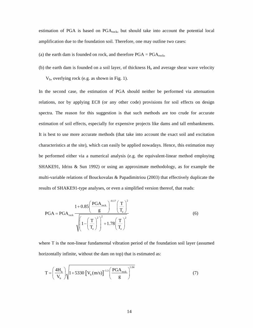
estimation of PGA is based on PGArock, but should take into account the potential local

amplification due to the foundation soil. Therefore, one may outline two cases:

(a) the earth dam is founded on rock, and therefore PGA = PGArock,

(b) the earth dam is founded on a soil layer, of thickness Hb and average shear wave velocity

Vb, overlying rock (e.g. as shown in Fig. 1).

In the second case, the estimation of PGA should neither be performed via attenuation

relations, nor by applying EC8 (or any other code) provisions for soil effects on design

spectra. The reason for this suggestion is that such methods are too crude for accurate

estimation of soil effects, especially for expensive projects like dams and tall embankments.

It is best to use more accurate methods (that take into account the exact soil and excitation

characteristics at the site), which can easily be applied nowadays. Hence, this estimation may

be performed either via a numerical analysis (e.g. the equivalent-linear method employing

SHAKE91, Idriss & Sun 1992) or using an approximate methodology, as for example the

multi-variable relations of Bouckovalas & Papadimitriou (2003) that effectively duplicate the

results of SHAKE91-type analyses, or even a simplified version thereof, that reads:

20.17

rock

erock 22 2

e e

PGA T1 0.85

g TPGA PGA

T T1 1.78

T T

−

+

= − +

(6)

where Τ is the non-linear fundamental vibration period of the foundation soil layer (assumed

horizontally infinite, without the dam on top) that is estimated as:

[ ]1.04

1.3b rockb

b

4H PGAT 1 5330 V (m/s)

V g−

= +

(7)

15

where the term in parentheses in front of the square root depicts the elastic fundamental

vibration period of the foundation soil layer.

3.2 Estimation of the non-linear fundamental period Το of the dam vibration (Step 2)

The fundamental period Το of dam vibration may be attained as the structural period which

yields the peak spectral amplification from the base of the dam up to its crest, i.e. the period

where the peak of the pertinent transfer function (in terms of elastic response spectra) is

observed. The elastic value Toe may be obtained by employing results from analyses with

very low PGA values (to ensure elastic response of all geomaterials), while the non-linear

value To requires employing results from analyses at the desired PGA level.

In terms of the proposed methodology, in order to estimate the non-linear fundamental period

Το of dam vibration, one needs first to estimate its elastic value, Τοe. A statistical analysis of

such values from the numerical analyses leads to:

0.75oe H(m)0.024(s)T = (8)

The accuracy of Eq. (8) is evident from Fig. 3, which illustrates the effect of the height H on

the value of the elastic fundamental (eigen)period Τoe of dam vibration. From an analytical

point of view, one may also estimate Toe from a simplification of the proposals of Dakoulas

& Gazetas (1985) that may read as:

soe V

H.T 62= (9)

where Vs is the average (elastic) shear wave velocity within the body of the dam. Given that

the Vs value is not known a priori, one may solve Eq. (9) for Vs, given Eq. (8) for Toe, a

procedure that leads to:

0.25s 108.3H(m)(m/s)V = (10)

16

In other words, the results of the parametric analyses show that the average (elastic) Vs

ranges from 230 to 360m/s for a dam with a clayey core, with the value increasing as the

height of the dam increases due to higher overburden stresses.

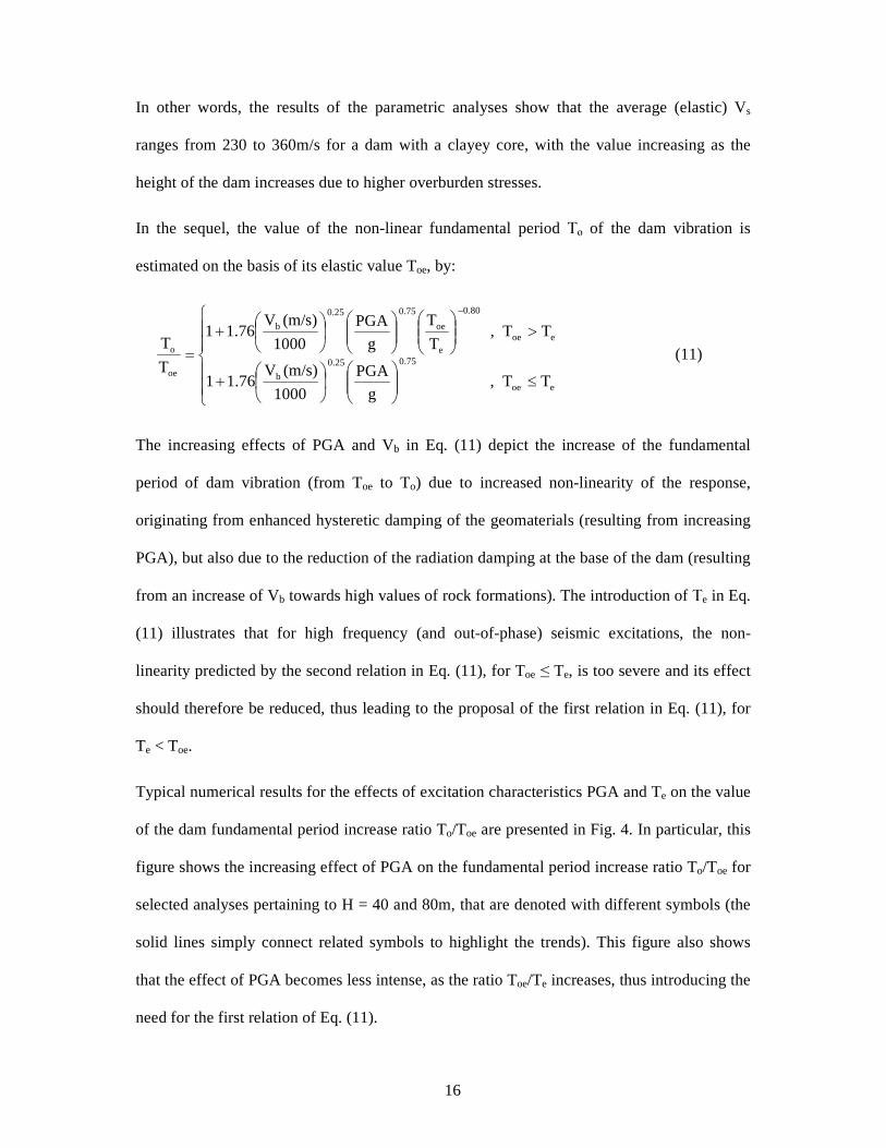
In the sequel, the value of the non-linear fundamental period Το of the dam vibration is

estimated on the basis of its elastic value Toe, by:

≤

+

>

+

=

−

eoe

0.750.25

b

eoe

0.80

e

oe

0.750.25

b

oe

o

TT,g

PGA

1000

(m/s)V1.76

TT,T

T

g

PGA

1000

(m/s)V1.761

T

T

1

(11)

The increasing effects of PGA and Vb in Eq. (11) depict the increase of the fundamental

period of dam vibration (from Toe to To) due to increased non-linearity of the response,

originating from enhanced hysteretic damping of the geomaterials (resulting from increasing

PGA), but also due to the reduction of the radiation damping at the base of the dam (resulting

from an increase of Vb towards high values of rock formations). The introduction of Τe in Eq.

(11) illustrates that for high frequency (and out-of-phase) seismic excitations, the non-

linearity predicted by the second relation in Eq. (11), for Toe ≤ Te, is too severe and its effect

should therefore be reduced, thus leading to the proposal of the first relation in Eq. (11), for

Te < Toe.

Typical numerical results for the effects of excitation characteristics PGA and Te on the value

of the dam fundamental period increase ratio To/Toe are presented in Fig. 4. In particular, this

figure shows the increasing effect of PGA on the fundamental period increase ratio To/Toe for

selected analyses pertaining to H = 40 and 80m, that are denoted with different symbols (the

solid lines simply connect related symbols to highlight the trends). This figure also shows

that the effect of PGA becomes less intense, as the ratio Toe/Te increases, thus introducing the

need for the first relation of Eq. (11).

17

The overall accuracy of Eq. (11) is evaluated in Fig. 5 against all the numerical results in the

database. In particular, each symbol in this figure corresponds to a different analysis and is

obtained using as coordinates, on one hand, the value of the dam fundamental period increase

ratio To/Toe from the analysis, and, on the other hand, the respective simulated value using

Eq. (11). A perfect prediction would locate the symbol on the diagonal of the figure (solid

line). The two dashed lines denote the standard deviation of the relative error in the

estimation of To/Toe, which in this case is equal to ±16%, depicting quite satisfactory

accuracy.

Finally note that based on Eqs (8) and (11), the methodology implies that reservoir

impoundment and the existence or not of stabilizing berms do not appear to affect the

fundamental period of dam vibration. The former because hydrodynamic pressures are not

important for mildly steeped slopes, while the latter because typical berms are not wide and

tall enough to effectively stiffen the overall dynamic response of the dam (Bouckovalas et al

2009, Andrianopoulos et al 2012).

3.3 Estimation of the peak acceleration at the dam crest, PGAcrest (Step 3)

By definition, the ratio of PGAcrest/PGA depicts the seismic amplification ratio, in peak value

terms, within the dam body, as compared to the outcropping foundation soil. In order to

consistently quantify this ratio and to effectively disregard local variations of seismic motion

at the very top of dams that are of little practical importance, the value of PGAcrest in this

paper is estimated as the maximum value of the resultant acceleration time history in the

upper 10% of the dam height. This consistently defined amplification ratio may be considered

similar in nature to amplification ratios related to 1D soil effects. As such, its value is

expected to be influenced by the non-linear fundamental period of dam vibration To, the

predominant period of the excitation Te and parameters related to the hysteretic damping of

18

the dam geomaterials and the radiation damping enabled by the stiffness of the foundation

layer at the base of the dam. Based on Papadimitriou et al. (2010), the correlation of the

PGAcrest/PGA ratio to the (tuning) period ratio To/Te, besides being consistent to 1D seismic

amplification ratios, also reduces the scatter of pertinent numerical results, as compared to

simpler correlations to To or height H alone. This correlation is corroborated by the numerical

data used in this effort, and therefore, the dam amplification ratio PGAcrest/PGA is estimated

by:

o o

e

ocrest

e

0.7

o o

e e

2 T, 0.5

T

TPGA , 0.5 1.5TPGA

2T T, 1.5

3T T

e

−

ΤΠ ≤

Τ Π ≤ ≤= Π ≤

(12a)

with:

0.52

b

1000

(m/s)V2.7Π

= (12b)

Based on Eq. (12a), the dam amplification ratio PGAcrest/PGA is estimated by a design

spectrum type relation, which has a fixed maximum value of Π, Eq. (12b), for a range of

predominant excitation periods Τe close to the non-linear fundamental period To of dam

vibration, while it reduces with an increase of the (tuning) period ratio To/Te, in a manner

reminiscent of acceleration design spectra in code provisions for buildings due to out-of-

phase vibration Obviously, for very short dams (very small To/Te values) the seismic

amplification also reduces, since the whole dam vibrates practically similarly to its base.

Furthermore, in principle, the value of Π, should be related to the two damping components,

of hysteretic (via PGA) and radiation (via Vb) type, just like it was performed in Step 2, Eq.

(11), for the fundamental period increase ratio To/Toe. Nevertheless, the analysis of the data

19

did not yield any statistically important effect of PGA on the value of PGAcrest/PGA in

general, or particularly on the value of Π. This is probably due to the fact that this effect is

already incorporated, to a large degree, via the use of To instead of Toe in Eq. (12), a

parameter that is strongly influenced by PGA (see exponent 0.75 in Eq. 11). On the contrary,

the same statistical analysis yielded a strong correlation of the value of Π to the shear wave

velocity Vb via Eq. (12b) that depicts the reduced seismic amplification within the dam body

if this is founded on a soft layer, as opposed to firm soil or rock conditions, due to an increase

of the related radiation damping. The need for this strong correlation is also implied by the

fact that the effect of radiation damping, via Vb, was not found equally important for the

estimation of To, since the pertinent exponent was just 0.25 in Eq. (11).

As an example, Fig. 6 presents a comparison of selected data (symbols) from the numerical

database, for the extreme cases of dams over foundation layers having Vb = 250m/s and

1500m/s, to the pertinent (solid line) predictions using Eq. (12). The data show that this effect

of radiation damping is very important indeed for the dam response (a factor of more than 2.5

near resonance), and also that for out-of-phase excitations (To > Te) the seismic amplification

within the dam body is reduced considerably in comparison to its maximum value for

excitations with predominant periods Te near the non-linear fundamental period To of the

dam. Moreover, Fig. 6 shows that Eq. (12) predicts both effects quite satisfactorily. It should

be underlined that Papadimitriou et al. (2010) did not have enough data to establish a relation

between PGAcrest/PGA and Vb and had simply proposed two relations, one for (really) soft

conditions with Vb = 250m/s and the other for firm ground or rock foundation with much

higher Vb values.

The overall accuracy of Eq. (12) is depicted in Fig. 7 against all the numerical results in the

database (in the format of Fig. 5). A satisfactory agreement is observed here with a standard

deviation of the relative error equal to ±27%.

20

Finally note that based on Eq. (12), the methodology implies that reservoir impoundment and

the existence or not of typical stabilizing berms do not appear to affect the PGAcrest values.

This is attributed to the same reasons that these parameters do not affect the fundamental

period of dam vibration To (see Section 3.2, and Andrianopoulos et al 2012 for details).

3.4 Estimation of peak seismic coefficient khmax as a function of PGAcrest (Step 4)

According to Makdisi and Seed (1978), the value of the peak seismic coefficient khmax may be

satisfactorily normalized over the peak acceleration at the dam crest PGAcrest, a parameter

that, based on Section 3.3), reflects the effects of excitation characteristics (PGA, Te), dam

geometry (To) and foundation conditions (Vb). Moreover, it is well established that for a fixed

dam-foundation-excitation combination, and therefore a fixed PGAcrest value, the khmax values

reduce as the maximum depth z (from the dam crest, see Fig. 1) of the failure surface

increases (Makdisi and Seed 1978, Papadimitriou et al. 2010). This because accelerations

generally decrease within the dam body as compared to the dam crest, but also because the

large sliding mass of a deep seated failure surface includes points that vibrate out-of-phase,

thus reducing the maximum value of the resultant acceleration of the sliding mass, that is

quantified via khmax. Yet, Andrianopoulos et al. (2012) showed that the design curve of

Makdisi and Seed (1978) for estimating the khmax/(PGAcrest/g) ratio as a reducing function of

the normalized maximum depth ratio z/H is qualitatively accurate, but is accompanied by

significant scatter and a clear bias of their proposal towards intermediate height H dams (40 –

80m).

To explore this effect of dam height H on the khmax/(PGAcrest/g) ratio, Fig. 8 focuses on a

subset of the numerical database, that corresponds to khmax/(PGAcrest/g) values for various

sliding masses pertaining to dams with height H = 20, 40 and 80m (denoted by different

symbols), founded on a stiff soil or soft rock layer (e.g. marl) with Vb = 500m/s and being

21

excited with mild intensity motions of PGA = 0.15g having exceptionally different

predominant periods, namely Te = 0.49sec (solid symbols) and Te = 0.15sec (hollow

symbols). Specifically, in Figure 8b, the khmax/(PGAcrest/g) values are correlated to the

normalized maximum depth ratio z/H, i.e. as proposed by Makdisi and Seed (1978). Careful

examination reveals that the effect of dam height H persists, while the solid symbols always

plot to the right of their respective hollow counterparts, clearly denoting that low frequency

motions (Te = 0.49sec) lead to higher khmax/(PGAcrest/g) values for the same failure surface, as

compared to high frequency motions (Te = 0.15sec). These consistent effects underline the

need for a new correlation.

Hence, in order to alleviate the bias in terms of dam height H, Fig. 8a simplifies the

correlation by introducing depth z as the design parameter, in a manner reminiscent of the

stress reduction factor rd in the liquefaction potential methodology of Youd and Idriss (2001).

Observe that the reducing effect of z is verified by the data, but the overall scatter is not

reduced. In addition, the consistent bias in terms of Te on the khmax/(PGAcrest/g) values

remains. Alternatively, Figure 8c explores the use of the predominant shear wavelength in the

dam body, denoted as λd, as the normalizing parameter of maximum depth z. In concept, this

type of normalization takes into account the fact that relatively large predominant shear

wavelengths λd lead to in-phase vibration of different locations within a sliding mass (of

maximum depth z) and therefore larger values of khmax/(PGAcrest/g), as compared to the

khmax/(PGAcrest/g) values pertaining to relatively small λd values but the same z. This trend is

indeed verified in Fig. 8c that shows a decreasing effect of the normalized maximum depth

ratio z/λd on the value of the kh/(amax,crest/g) ratio, with relatively small scatter and no

consistent bias (neither in terms of H, nor in terms of Te).

It should be noted that λd is not known a priori, since it is a function of the nonlinear shear

wave velocity Vsd and the predominant period of vibration Td within the dam body. The

22

former may be related to To by using Eq. (9) for nonlinear properties (To and Vsd instead of

Toe and Vs). On the contrary, the predominant period of vibration Td is a new parameter that

is equal neither to the predominant excitation period Te, nor to the nonlinear fundamental

period To of dam vibration. In practice, Td usually takes values in between Te and To and

therefore it is assumed to be approximately equal to their average value. Following this train

of thought, λd may be approximated as follows:

+=

+==

o

eeo

odsdd T

T11.3H

2

TT

T

2.6HTVλ (13)

This relation for λd was used in the correlation of Fig. 8c, and was also used in the pertinent

statistical regression of the whole database. In particular, this regression corroborated the

generally decreasing effect of the maximum depth ratio z/λd, but also depicted a number of

other significant effects. In particular, based on the proposed methodology, the khmax may be

estimated on the basis of PGAcrest (from Step 3) and z/λd according to:

hmaxl b f g

crest d

k zC 1.18C C C

PGA /g λ

= −

(14a)

with:

hmaxb f g

crest

k1.0 0.65C C C 1.0

PGA /g

− ≤ ≤

(14b)

where the various C coefficients included in Eq. (14) are related to the (upstream or

downstream) location of the sliding mass (Cl), large stabilizing berms (Cb), the stiffness of

foundation layer (Cf) and geometric characteristics of the sliding mass (Cg) other than

maximum depth z, as explained in the sequel.

Figure 9 illustrates the so-called “fundamental” relation of khmax/(PGAcrest/g) reduction with

the normalized maximum depth ratio z/λd of the sliding mass that is based on, the also

23

presented, pertinent numerical data. The term “fundamental” relation used here denotes that

all C coefficients of Eq. (14) are taken equal to 1.0, thus leading to presentation of only the

pertinent numerical data in Fig. 9, i.e. the data that correspond to cases where the dam is

founded on stiff soil or any type of rock (Vb ≥ 500m/s) and does not have typical stabilizing

berms, or if it does have such berms the sliding masses are shallow and do not include them

(practically leading to z < 0.67Η for the performed analyses). In addition, the presented data

correspond to “bulky” (and not “thin”) sliding masses (see definitions below), which are not

in contact to the reservoir water (if this exists), i.e. for analyses that correspond to earthquake

loading at the end of construction, and for downstream sliding masses in the case of a full

reservoir (steady state seepage conditions). Observe the relatively small scatter of the data

and the fact that the reducing effect of z/λd saturates at khmax/(PGAcrest/g) = 0.35, which poses

as a lower limit, and requires the introduction of an inequality at the left hand side of Eq.

(14b).

From the effects introduced via the C coefficients in Eq. (14), the emphasis is put now on the

effect of reservoir impoundment. In particular, Fig 10 presents numerical data in the

khmax/(PGAcrest/g) versus z/λd format, for upstream sliding masses, that would otherwise be

considered as corresponding to the “fundamental” relation, namely Cb = Cf = Cg = 1.0.

Therefore, Fig. 10 also includes the “fundamental” relation of Fig. 14 and shows that the

upstream data plot above but in parallel to the “fundamental” relation. Hence, a best-fit

average relation for these data can be established by a mere translation of the decreasing

curve to larger values of khmax/(PGAcrest/g), thus giving birth to coefficient Cl in Eq. (14a).

Moreover, the fact that khmax/(PGAcrest/g) never exceeds 1.0, yielded the need for including

the inequality at the right hand side of Eq. (14b), of significance only for upstream sliding

masses.

24

By performing similar data selection and statistical analysis, the following values or relations

for the C “correction” coefficients were hereby estimated:

• Cl is the location coefficient, which takes a value of 1.08 for upstream sliding masses of

an impounded dam, and a value of 1.0 in any other case. Note that the relatively higher

khmax values for upstream sliding masses are attributed to amplification phenomena in the

pertinent shell due to the stiffness contrast between the saturated (and hence softer)

upstream shell as compared to the non-saturated (and hence stiffer) downstream shell of a

zoned earthdam at conditions of steady state seepage.

• Cb is the berm coefficient, which takes a value of 0.96 if the sliding mass includes a

typical stabilizing berm, and a value of 1.0 in any other case. It should be noted that the

slightly higher khmax values for sliding masses that include a typical stabilizing berm are

attributed to topographic amplification phenomena observed in the vicinity of such berms,

similarly to what is observed near any single-faced slope of related dimensions (e.g.

Bouckovalas and Papadimitriou 2005). Yet, these effects are practically local and do not

affect consistently the overall dam response (e.g. values of To and PGAcrest remain

essentially unaffected, see Bouckovalas et al. 2009, Andrianopoulos et al 2012)

• Cf is the foundation coefficient, which is given by:

≥

<

+

=

500m/sV,1.00

500m/sV,1000

(m/s)V1.240.38

C

b

bb

f (15)

The form of Eq. (15) denotes that there is a small consistent amplifying effect on

khmax/(PGAcrest/g) values for earth dams founded on a soft soil layer (of significant

thickness, i.e. more than 5m). Note that low Vb values (leading to Cf < 1) are considered

practically possible only for relatively short dams (e.g. H ≤ 30m). This is due to the fact

25

that for taller earthdams a relatively soft foundation layer could make the construction of

the dam problematic (e.g. excessive settlements).

• Cg is the geometry coefficient of the sliding mass, which is given by:

g

0.91 , if (t/w) 0.14 (i.e. for " "sliding mass)C

1.00 , if (t/w) 0.14 (i.e. for " " sliding mass)

thin

bulky

≤=

> (16)

with the w and t being geometrical characteristics of the sliding mass, corresponding to its

width (in the horizontal direction) and the maximum distance between two lines that are

parallel to the points of entry and exit of the failure surface and adjoin the sliding mass

(see Fig. 1, for illustrated definition). Obviously, small (t/w) ratios correspond to

relatively elongated thin sliding masses, thus the use of the term “thin” in Eq. (16), while

for large (t/w) ratios the sliding masses are relatively bulky, thus the homonymous term in

Eq. (16). The relatively higher values of khmax for “thin” as opposed to “bulky” sliding

masses with the same maximum depth z are attributed to the fact that the former include

mostly surficial locations of the dam body where higher accelerations are expected as

compared to the heavier latter sliding masses.

Figure 11 evaluates the overall accuracy in the prediction of the peak seismic coefficient

khmax for all 1084 sliding masses in the numerical database. A satisfactory accuracy is

depicted with a standard deviation of the relative error equal to ±27% (see dashed lines). In

order to fully ascertain the appropriateness of the proposed methodology, Fig. 12 studies the

relative error in the prediction of khmax, denoted as R_khmax, which is defined as the ratio of

the difference of the predicted value of khmax minus the khmax from the analyses over the latter

value. Hence, positive values of R_khmax correspond to overprediction, while negative to

underprediction of the peak seismic coefficient. In particular, this figure plots the R_khmax

values for all 1084 sliding masses against the (tuning) period ratio To/Te (in plot a), the

normalized maximum depth ratio z/λd (in plot b) and the PGA (in plot c), while different

26

symbols denote different dam heights H. It is thus observed that there is no consistent bias of

overprediction or underprediction for any of the important problem parameters.

4. ESTIMATION OF EFFECTIVE SEISMIC COEFFICIENT khE ON THE

BASIS OF ALLOWABLE DISPLACEMENTS

The previous section described a stand-alone, user-friendly methodology for estimating the

peak seismic coefficient khmax, given the excitation characteristics (PGArock, Te), the

foundation conditions (Hb, Vb), the characteristics of the dam (H, Vs) and of the sliding mass

(z, w, t, location, etc). In this section, a methodology will be proposed for estimating the

“effective” seismic coefficient khE (for use in pseudo-static analyses) as a percentile of its

peak value, on the basis of:

khE = khmax / q (17)

where q (≥ 1) is the sliding factor that is to be correlated to allowable downslope deviatoric

displacements Dall.

To do so, one may assume that the slope is at a state of limit equilibrium (FSd = 1.0) when the

inertial acceleration is equal to khEg, i.e. khE = ky. In this way, and given Eq. (17), the slope is

allowed to develop downslope deviatoric displacements, since the peak acceleration of the

sliding mass khmaxg corresponds to FSd < 1. The amount of these displacements may be

estimated using Newmark’s sliding block procedure, given khmax and ky. Here, the opposite is

required, namely to correlate the q = khmax/ky to the given allowable downslope deviatoric

displacements Dall. For this purpose one may employ any of the (many) displacement

equations for sliding blocks available the literature and solve for ky, i.e. the only parameter

that is common in all equations. This train of thought was followed by Bray and Travasarou

(2009), who employed the equation of Bray and Travasarou (2007) that was based on

27

“coupled” analyses. In this effort, the analyses performed were “decoupled” and therefore,

for consistency, the few available displacement equations/charts that are based on

“decoupled” analyses (Makdisi and Seed 1978, Bray and Rathje 1998) were entertained as

initial options. However, none of them was finally opted, since the former uses a non-

engineering parameter (earthquake magnitude M) in its formulation and was based on

relatively few recordings available at that time, while the latter uses the PGArock as an

intensity measure, which is related to the base excitation but not the actual dam vibration.

Then, the large family of rigid sliding block displacement equations was considered as a pool

for selecting an appropriate equation. The basic premise here is that such an equation may be

accurately used for a flexible sliding block, if the seismic intensity measures accounted for in

the equation are not those of the plane (e.g. PGA, PGV), but of the sliding block itself (e.g.

ahmax=khmaxg, peak velocity of the sliding mass vhmax, respectively) estimated on the basis of

the “decoupled” analyses. It is well known that this family of equations employs many

different types and combinations of intensity measures: PGA (common in practically all

equations), PGV (e.g. Newmark 1965, Franklin and Chang 1977, Richards and Elms 1979,

Whitman and Liao 1984, Cai and Bathurst 1996, Saygili and Rathje 2008), predominant

period Te (e.g. Sarma 1975, Ambraseys and Menu 1988, Yegian et al. 1991), Arias intensity

Ia (Jibson 2007), and in some cases the earthquake magnitude M (e.g. Saygili and Rathje

2008) or even the number of significant excitation cycles N (e.g. Yegian et al 1991). Hence,

in the selection process, it was considered essential to consider equations including PGV (in

order to take into account the frequency content of the excitation), and to avoid equations that

employ parameters that are non-engineering (M) and not so well-established in engineering

practice (Ia, N).

Figure 13 compares the range of displacement D predictions from the parametric study of

Franklin and Chang (1977) to a series of equations that meet the foregoing criteria (and are

28

provided in Table 1), namely:

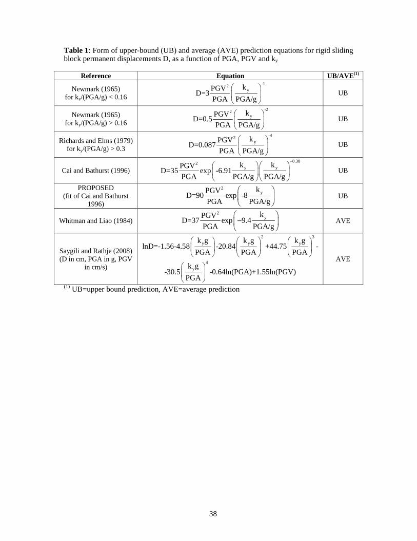
o several upper-bound (UB) equations: Newmark (1965), Richards and Elms (1979), Cai

and Bathurst (1996), and

o one average (AVE) equation: Whitman and Liao (1984).

Note that the employed plotting scheme normalizes displacements D with parameter

PGV2/PGA (that also measures in m), while the horizontal axis plots the ratio of ky/(PGA/g)

and provides generalization for all possible combinations of ky, PGA and PGV. Hence, other

equations that also meet the previously set criteria (e.g. Saygili and Rathje 2008; see Table 1),

but are unable to be plotted and compared in Fig. 13 due to the selected generalization

scheme, had to be excluded from the pool of options.

Based on this figure it may be concluded that the equation of Whitman and Liao (1984) is

considered appropriate for an average fit of the depicted range of sliding block displacement

predictions, while the equation of Cai and Bathurst (1996) is considered appropriate for an

upper bound fit. Note that, if one replaces PGA with khmaxg and PGV with vhmax in any of the

equations of Table 1, he may then attempt to solve for ky or better directly for the sliding

factor q = khmax/ky. This can be readily done for the equation of Whitman and Liao (1984),

but not for the equation of Cai and Bathurst (1996). Hence, the latter was replaced with the

one denoted as “proposed” in Figure 13 and Table 1, that fits it with a simpler analytical

form. Doing so yields the following equations for upper bound qUB and average qAVE

estimates of the sliding factor:

UB2hmax

allhmaxhmax

hEAVE2

hmaxall

hmax

-8(=q ), for conservatism

vln D 90

k gkq= = 1

-9.4k(=q ), for averageestimates

vln D 37

k g

≥

(18)

29

The graphical form of qUB and qAVE is presented in Fig. 14. Focusing first on qUB it becomes

obvious that qUB = 1 for very small displacements, Dall < 0.03[vhmax2/(khmaxg)], and exceeds a

value of 2 for quite larger displacements Dall > 1.65[vhmax2/(khmaxg)]. Furthermore, note that

always qAVE > qUB for the same value of allowable displacements Dall, i.e. the khE values are

larger when employing qUB rather than qAVE for the same khmax, thus leading to more

conservative design. Careful examination of Eq. (18) shows that the ratio of qAVE/qUB ranges

between 1.3 and 2, and exceeds 2 only for extremely large values of Dall >

10.44[vhmax2/(khmaxg)]. It should be underlined that although this figure has been drawn for q

values up to 10, it is not advised to use such large values in the design of earthdams due to

the crudeness of employing rigid sliding block equations for such large overall downslope

displacements.

Note that a similar assumption was recently used by Rathje and Antonakos (2011) who

replaced PGA and PGV of the rigid sliding block displacement equation of Saygili and

Rathje (2008) with khmaxg and vhmax from “coupled” analyses in order to estimate flexible

sliding mass displacements. In their effort, they show that such an approach is rational, but it

may underestimate displacements for very flexible sliding masses. This may be attributed to

the fact that their khmax/(PGA/g) ratios usually fall significantly below 1.0 for flexible sliding

masses (may reach values of 0.1, on average, for very flexible masses). This is not observed

in data from “decoupled” analyses, which show values for the khmax/(PGA/g) ratio that are

consistently below 1.0, on average, only for deep sliding masses (z/H > 0.7) and especially

for out-of-phase dam vibrations (To/Te > 2), but even then, this ratio does not reach values

30

lower than 0.4, on average (e.g. Andrianopoulos et al. 2012). In any case, the use of qUB

rather than qAVE of Eq. (18), along with a “decoupled” estimation of khmax in Section 3 may

be considered sufficient to alleviate all concerns regarding non-conservatism of the proposed

methodology.

The only parameter not quantified in Eq. (18) is the value of vhmax, i.e. the peak velocity of

the sliding mass. This will not be estimated as a separate quantity; but through the ratio of the

peak velocity over the peak acceleration of the sliding mass (vhmax/ahmax) a quantity that may

be related to the vibration period of the sliding mass, similarly to how the PGV/PGA ratio is

related to the predominant period Te of a seismic recording (e.g. Te = 4.3(PGV/PGA)

according to Fajfar et al. 1992). By relating this ratio to the predominant period of dam

vibration Td = (To + Te)/2 (see Eq. 13) and the normalized maximum depth of the sliding

mass (z/λd), a statistical regression of numerical data yielded the following equation:

[ ]0.12

hmax hmaxd

hmax hmax d

v v z(sec) = (sec)=0.071 1+1.48T

a k g λ

(19)

This relation shows that the (vhmax/ahmax) ratio increases practically linearly with an increase

in the significant periods Τe and Το of the problem, and that it also increases slightly as the

sliding mass becomes deeper, and thus more flexible. Figure 15 presents the overall accuracy

in the prediction of the ratio (vhmax/ahmax), and thus of the peak velocity of the sliding mass

vhmax, for all 1084 sliding masses in the numerical database. Based on this, a very satisfactory

accuracy is depicted with a standard deviation of the relative error equal to ±19%.

31

5. DISCUSSION

Despite significant research invested to estimating seismic coefficients for the design of

earthdams and tall embankments, there is still need for a methodology that establishes a

correlation between the well-established pseudo-static analysis of such geostructures and

modern performance-based design principles. The hereby proposed methodology is based on

statistical analysis of input data and results from “decoupled” seismic response analyses and

is stand-alone, i.e. it provides end-results without resorting to other methodologies.

Furthermore, it is simple, as it may be programmed in a worksheet, and leads to satisfactory

accuracy in the estimation of the peak seismic coefficient khmax with a standard deviation of

the relative error equal to ±27% in comparison to case-specific non-linear numerical

analyses. To allow for the performance-based seismic design of earthdams, a sliding factor q

(≥1) is defined that divides the khmax value to yield the “effective” seismic coefficient khE,

which is to be used for pseudo static analyses with a requirement of FSd ≥ 1.0. The value of

the sliding factor is estimated on the basis of allowable slope displacements Dall, peak seismic

intensity indices for the sliding mass (peak acceleration ahmax and velocity vhmax) and the

desired level of conservatism (upper-bound or average).

The basic premise of the proposed methodology for estimating khmax is the use of

“decoupled”, and not “coupled” analyses for its purpose. This choice may come as a surprise,

given that the latter analyses are currently the state-of-the-art for slope stability issues, with

many benefits arising from their use (e.g. less computational effort). Nevertheless, the former

type of analyses comprises the state-of-practice world-wide (e.g. Rathje and Antonakos

2011), especially for earthdams. Moreover, only such analyses give emphasis to aspects of

dam vibration (e.g. effects of dam resonance (for To/Te ≅ 1) and soil foundation stiffness) that

have been proven to be significant for the values of khmax (e.g. Zania et al 2011,

Papadimitriou et al. 2010, Andrianopoulos et al. 2012). In addition, it was desired to

32

investigate whether typical stabilizing berms and reservoir impoundment affect the values of

the seismic coefficients of earthdams, as well to ascertain the relative importance of the exact

geometry of the sliding mass (besides its maximum depth z), all issues that could only be

addressed by “decoupled” analyses. The foregoing benefits of using “decoupled” analyses

come at a price of conservatism for sliding masses of shallow and intermediate depth, but

also a tendency for non-conservatism for flexible (deep) sliding masses, and this especially

for high ratios of ky/khmax (e.g. Kramer and Smith 1997, Rathje and Bray 2000). Focusing on

the latter problem (which is of main concern for practitioners), it is important to note that this

non-conservatism is generally related to small displacements, due to the high values of

ky/khmax mentioned above, in combination with small values of khmax observed for flexible

masses (Rathje and Antonakos 2011). Hence, the use of a “decoupled” approach may be

considered “reasonably accurate” for flexible sliding masses, an assertion independently

confirmed by experimental work (Wartman et al. 2003). In any case, as far as the proposed

methodology is concerned, the end-user may partly adjust the desired level of conservatism

when selecting the sliding factor q, i.e. values of qUB or qAVE or anything in between,

although the use of qUB is recommended by the authors, at least for preliminary design stages.

Overall, the methodology is considered reliable for use in the design of:

(a) Earthdams or tall embankments, with height H ranging from 20 to 120m, of triangular

or trapezoidal cross section, with or without typical stabilizing berms (e.g. of height and

width up to H/3 and 2H/3), for end of construction and steady state seepage conditions, that

are founded on ground with shear wave velocities Vb higher than 250m/s (firm soil or rock),

(b) Seismic excitations with predominant periods Τe = 0.14 to 0.50s and peak

accelerations PGA at the free-field of the foundation soil reaching up to 0.50g.

33

Of interest is also the fact that the methodology is applied in independent steps of generic

value, given the parametric nature of the performed analyses. Specifically, if one has

independently estimated the PGA (Step 1, section 3.1) or even the non-linear fundamental

period To of a geostructure (Step 2, section 3.2), he may apply only the remaining Steps 3 and

4 for estimating the peak seismic coefficient khmax, without loss of accuracy. Also, specific

steps of the methodology may be used in aid of other existing methodologies (e.g. Step 3 for

estimating the PGAcrest may be used in combination with the Makdisi and Seed 1978

procedure, which does not explicitly provide an equation or design chart for its estimation).

Given that the methodology was based on plane strain analyses, the earthdam or tall

embankment in question should be sufficiently long as to allow for an accurate 2D

approximation. Moreover, ground movements (e.g. crest settlements) due to volumetric

densification are not captured by Newmark-type models. Hence, the Dall to be used in this

methodology to estimate the sliding factor q should refer only to deviatoric-induced

displacements, while densification-induced displacements should be accounted for separately,

on the basis of relevant methodologies (e.g. Tokimatsu and Seed 1987). Furthermore, the

methodology emphasizes on seismic coefficients related to the horizontal sliding mass

vibration, and there is no reference made to the vertical component of motion. This is

consistent with all pertinent methodologies in the literature, both “coupled” and “decoupled”,

but is also backed by recent evidence (Christchurch earthquake) showing that for sliding

systems even large vertical acceleration components have only a negligible effect (Gazetas et

al 2012). Finally, it should be underlined that the performed analyses, as well as the proposed

methodology, do not take into account shear strength degradation of the geomaterials

comprising the earthdam. The literature includes elegant and simple procedures for

incorporating such issues in seismic slope stability analyses (e.g. Biondi et al. 2002

incorporate the effects of excess pore pressure buildup in assessing the stability of infinite

34

cohessionless slopes). Yet, given the complexity of such issues and the importance of

infrastructure works like earthdams or tall embankments, the authors believe that robust

numerical analyses with advanced constitutive models (e.g. NTUA-SAND of

Andrianopoulos et al. 2010 for liquefiable soils) should remain the seismic analysis tool for

such geostructures.

6. ACKNOWLEDGEMENTS

The authors would like to thank the Public Power Corporation of Greece S.A. for funding this

research, as well as Civil Engineers Angelos Zographos, Sofia Tsakali and Stavroula Stavrou

for performing the numerical analyses on which the proposed methodology was based.

7. REFERENCES

1. Ambraseys N. N., Menu J. M. (1988), “Earthquake-induced ground displacements”, Earthquake Engineering and Structural Dynamics, Vol. 16, pp. 985–1006

2. Andrianopoulos K. I. (2006), “Numerical modeling of static and dynamic behavior of elastoplastic soils, Doctorate Thesis, Department of Geotechnical Engineering, School of Civil Engineering, National Technical University of Athens (in Greek)

3. Andrianopoulos K. I., Papadimitriou A. G., Bouckovalas G. D. (2010), “Bounding surface plasticity model for the seismic liquefaction analysis of geostructures”, Soil Dynamics and Earthquake Engineering, Vol. 30, No. 10, pp. 895-911

4. Andrianopoulos K. I., Papadimitriou A. G., Bouckovalas G. D., Karamitros D. K. (2012), “Insight to seismic response of earthdams, with emphasis on seismic coefficient estimation”, Computers and Geotechnics (under review)

5. Biondi G., Cascone E., Maugeri M. (2002), “Flow and deformation failure of sandy slopes”, Soil Dynamics and Earthquake Engineering, 22(9-12): 1103-1114

6. Biondi G., Cascone E., Rampello S. (2007), “Performance-based pseudo-static analysis of slopes”, 4th International Conference on Earthquake Geotechnical Engineering, Thessaloniki, Greece, June 25-28

7. Bouckovalas G. D., Papadimitriou A. G. (2003), “Multi-variable relations for soil effects on seismic ground motion”, Earthquake Engineering and Structural Dynamics, 32: 1867-1896, Wiley

35

8. Bouckovalas G. D., Papadimitriou A. G. (2005), “Numerical Evaluation of Slope Topography Effects on Seismic Ground Motion", Soil Dynamics and Earthquake Engineering, 25(7-10): 547 - 555

9. Bouckovalas G. D., Papadimitriou A. G., Andrianopoulos K. I. (2009), “Estimation of seismic coefficients for the slope stability of earthdams: Phase B”, Research Report to Public Power Corporation, p. 269 (in Greek)

10. Bozbey I., Gundogdu O. (2011), “A methodology to select seismic coefficients based on upper bound “Newmark” displacements using earthquake records from Turkey”, Soil Dynamics and Earthquake Engineering, 31, 440-451

11. Bray J. D., Rathje E. M. (1998), “Earthquake-induced displacements of solid-waste landfills”, Journal of Geotechnical and Geoenvironmental Engineering, ASCE 124 (3), 242–253

12. Bray J. D., Travasarou T. (2007), “Simplified procedure for estimating earthquake –induced deviatoric slope displacements”, Journal of Geotechnical and Geoenvironmental Engineering, ASCE, 133(4):381-392

13. Bray J. D., Travasarou T. (2009), “Pseudostatic coefficient for use in simplified slope stability evaluation”, Journal of Geotechnical and Geoenvironmental Engineering, ASCE, 135(9):1336-1340

14. Cai Z., Bathurst R. J. (1996), “Deterministic sliding block methods for estimating seismic displacements of earth structures”, Soil Dynamics and Earthquake Engineering, 15, 255-268

15. Charles J. A., Abiss C. P., Gosschalk E. M., Hinks J. L. (1991), “An engineering guide to seismic risk to dams in the United Kingdom”, Building Research Establishment Report.

16. Dakoulas P., Gazetas G. (1985). “A class of inhomogeneous shear models for seismic response of dams and embankments”, Soil Dynamics and Earthquake Engineering, 4(4): 166-182

17. Fajfar P, Vidic T, Fischinger M. (1992), “On energy demand and supply in SDOF systems”. In Nonlinear Seismic Analysis of RC Buildings, Fajfar P, Krawinkler H. (eds). Elsevier: Amsterdam, 41-61.

18. Franklin A. G., Chang F. K. (1977), “Permanent displacement of earth embankments by Newmark sliding block analysis”, Misc. Paper S-71-17, Soil and Pavement Labs, US Army Eng. Waterways Expt. Stn., Vicksburg, Miss.

19. Gazetas, G., Garini, E., Berrill, J. B., Apostolou, M. (2012), “Sliding and overturning potential of Christchurch 2011 earthquake records”, Earthquake Engineering and Structural Dynamics, doi: 10.1002/eqe.2165

20. Hynes-Griffin M. E., Franklin A. G. (1984), “Rationalizing the seismic coefficient method”, Miscellaneous Paper GL-84-13, U.S. Army Corps of Engineers Waterways Experiment Station, Vicksburg, Mississippi, 21 pp

21. Idriss I. M., Sun J. I. (1992), “SHAKE91 – A computer program for conducting equivalent linear seismic response analysis of horizontally layered soil deposits. User’s Guide”, Center for Geotechnical Modeling, Civil Engineering Department, U.C. Davis

22. Itasca Consulting Group Inc (2005), “FLAC – Fast Lagrangian Analysis of Continua”, Version 5.0, User’s Manual.

36

23. Jibson R. W. (2007), “Regression models for estimating coseismic landslide displacement”, Engineering Geology, 91:209–18

24. Kramer S. L., Smith, M. W. (1997), “Modified Newmark model for seismic displacements of compliant slopes’’ Journal of Geotechnical and Geoenvironmental Engineering, 123(7): 635–644

25. Lin J.-S., Whitman, R. V. (1983), “Decoupling approximation to the evaluation of earthquake induced plastic slip in earth dams”, Earthquake Engineering and Structural Dynamics, 11, 667–678.

26. Makdisi F. H., Seed H. B. (1978), “Simplified procedure for estimating dam and embankment earthquake-induced deformations”, Journal of Geotechnical Engineering Division, ASCE, 104(7): 849-867

27. Newmark N. (1965), “Effects of earthquakes on dams and embankments”, Geotechnique, 15(2): 139-160

28. Papadimitriou A. G. (1999), “Elastoplastic modelling of monotonic and dynamic behavior of soils”, Doctorate Thesis, Department of Geotechnical Engineering, Faculty of Civil Engineering, National Technical University of Athens, June, (in Greek)

29. Papadimitriou A. G., Andrianopoulos K. I., Bouckovalas G. D., Anastasopoulos K. (2010). “Improved methodology for the estimation of seismic coefficients for the pseudo-static stability analysis of earthdams”, Proceedings, 5th International Conference on Recent Advances in Geotechnical Earthquake Engineering and Soil Dynamics, May 24-29

30. Ramberg W., Osgood W. R. (1943), “Description of stress-strain curve by three parameters”, Technical note 902, National Advisory Committee for Aeronautics

31. Rathje E. M., Antonakos G. (2011). “A unified model for predicting earthquake-induced sliding displacements of rigid and flexible slopes”, Engineering Geology, Vol. 122, pp. 51-60

32. Rathje E. M., Bray J. D. (2000), “Nonlinear coupled seismic sliding analysis of earth structures”, J. of Geotech. and Geoenviron. Engineering, ASCE, 126(11):1002-1014

33. Richards R., Elms D. G. (1979), “Seismic behaviour of gravity retaining walls”, Journal of Geotechnical Engineering Division, ASCE, 105(4), pp. 449-464

34. Sarma S. K. (1975), “Seismic stability of earth dams and embankments”, Geotechnique, 25(4): 743-761

35. Saygili G., Rathje E. M. (2008), “Empirical predictive models for earthquake-induced sliding displacements of slopes”, Journal of Geotechnical and Geoenvironmental Engineering, ASCE 134 (6), 790–803

36. Tokimatsu, K., Seed Η. Β. (1987), “Evaluation of settlements in sands due to earthquake shaking”, Journal of Geotechnical Engineering, ASCE, 113(8): 861-878

37. USCOLD (1985) “Guidelines for selecting seismic parameters for dam projects”, Report of Committee on Earthquakes, U.S. Committee on Large Dams

38. Vucetic M., Dobry R. (1991), “Effect of soil plasticity on cyclic response”, Journal of Geotechnical Engineering, ASCE, 117(1):89-107

39. Wartman J., Bray J. D., Seed R. B. (2003), “Inclined plane studies of the Newmark sliding block procedure”, Journal of Geotechnical and Geoenvironmental Engineering, ASCE, 129(8): 673-684

37

40. Whitman R. V., Liao S. (1984), “Seismic design of gravity retaining walls”, Proceedings, 8th World Conference on Earthquake Engineering, San Francisco, 3, pp. 533-540.

41. Youd T. L., Idriss I. M. (2001), “Liquefaction resistance of soils: summary report from the 1996 NCEER and 1998 NCEER/NSF Workshops on Evaluation of Liquefaction Resistance of Soils”, Journal of Geotechnical and Geoenvirnomental Engineering, ASCE, 127(4): 297 – 313

42. Yegian M. K., Marciano E. A., Ghahraman V. G. (1991), “Earthquake-induced permanent deformations: probabilistic approach”, Journal of Geotechnical Engineering, ASCE, 117(1): 1158-1167

43. Zania V., Tsompanakis Y., Psarropoulos P. N. (2011), “Seismic slope stability of embankments: a comparative study on EC8 provisions”, Proceedings, ERTC-12 Workshop on Evaluation of Geotechnical Aspects of EC8, Athens, Sept. 11, (ed. M. Maugeri), Patron Editore – Quarto Inferiore – Bologna.

38

Table 1: Form of upper-bound (UB) and average (AVE) prediction equations for rigid sliding block permanent displacements D, as a function of PGA, PGV and ky

Reference Equation UB/AVE(1)

Newmark (1965) for ky/(PGA/g) < 0.16

-12ykPGV

D=3PGA PGA/g

UB

Newmark (1965) for ky/(PGA/g) > 0.16

-22ykPGV

D=0.5PGA PGA/g

UB

Richards and Elms (1979) for ky/(PGA/g) > 0.3

-42ykPGV

D=0.087PGA PGA/g

UB

Cai and Bathurst (1996)

0.382y yk kPGV

D=35 exp -6.91PGA PGA/g PGA/g

−

UB

PROPOSED (fit of Cai and Bathurst

1996)

2ykPGV

D=90 exp -8PGA PGA/g

UB

Whitman and Liao (1984) 2

ykPGVD=37 exp 9.4

PGA PGA/g

−

AVE

Saygili and Rathje (2008) (D in cm, PGA in g, PGV

in cm/s)

2 3

y y yk g k g k glnD=-1.56-4.58 -20.84 +44.75 -

PGA PGA PGA

4

yk g-30.5 -0.64ln(PGA)+1.55ln(PGV)

PGA

AVE

(1) UB=upper bound prediction, AVE=average prediction

39

List of Figures Figure 1: Definition of critical geometric and geotechnical parameters for seismic slope

stability of earth dams and tall embankments

Figure 2: Calibration of model constants α1 and γ1 of employed non-linear hysteretic soil model (Eqs 1 through 5) to fit the experimental curves for shear modulus G/Gmax degradation and hysteretic damping ξ increase with cyclic shear strain γ of Vucetic and Dobry (1991)

Figure 3: Effect of height H on the elastic (first) eigen-period Toe of the dam

Figure 4: Typical numerical results for the effects of excitation characteristics (PGA and Te) on the dam fundamental period increase ratio (Το/Τoe) due to non-linearity

Figure 5: Prediction accuracy of the dam fundamental period increase ratio (Το/Τoe) due to non-linearity, against all numerical data

Figure 6: Examples of variability of dam amplification ratio PGAcrest/PGA, as a function of (tuning) period ratio To/Te and the shear wave velocity Vb (stiffness) of the foundation soil layer

Figure 7: Prediction accuracy of the dam amplification ratio PGAcrest/PGA ratio, against all numerical data

Figure 8: Correlations of khmax/(PGAcrest/g) ratio with different possible expressions of the maximum depth z of the sliding mass (data from analyses with PGA =0.15g, Vb = 500m/s)

Figure 9: Proposed “fundamental” relation of khmax/(PGAcrest/g) ratio versus normalized maximum depth ratio z/λd, as per Eq. (14) for Cl=Cb=Cf=Cg=1.0, against related numerical data

Figure 10: Effect of dam reservoir on the khmax/(PGAcrest/g) versus z/λd relation of the upstream sliding masses on the basis of numerical data, and comparison to the “ fundamental” relation of Eq. (14) for Cl=Cb=Cf=Cg=1.0

Figure 11: Prediction accuracy of the peak seismic coefficient khmax for sliding masses, against all numerical data

Figure 12: Effects of important problem parameters To/Te, z/λd and PGA on the relative error of khmax prediction for all numerical data

Figure 13: Permanent deviatoric slope displacements D as a function of ky, PGA and PGV from various upper bound (UB) and average (AVE) relations based on the rigid sliding block theory

Figure 14: Correlation of sliding coefficient q to allowable displacement Dall and peak seismic intensity measures of the sliding mass khmax and vhmax on the basis of upper bound (qUB) and average (qAVE) displacement equations

Figure 15: Prediction accuracy of the (vhmax/ahmax) ratio of sliding masses, against all numerical data

40

Figure 1: Definition of critical geometrical and geotechnical parameters for seismic slope

stability of earth dams and tall embankments

Single column

Figure 2: Calibration of model constants α1 and γ1 of employed non-linear hysteretic soil model (Eqs 1 through 5) to fit the experimental curves for shear modulus G/Gmax degradation and hysteretic damping ξ increase with cyclic shear strain γ of Vucetic and Dobry (1991)

Single column

bedrock

PGArock

PGAcrest

Fh = khW

Η

z

w

t

foundation soil layer (Vb) Ηb

PGA

0

0.2

0.4

0.6

0.8

1

G /

Gm

ax

0.0001 0.001 0.01 0.1 1cyclic shear strain γ (%)

0

5

10

15

20

25

ξ (%

)

γ1(%) 0.016 0.027 0.058PI(%) 0 15 30

Vucetic & Dobry (1991)for PI = 0 - 200%

model simulations(all with α1=0.64)

γ1(%) 0.15 0.33 0.6PI(%) 50 100 200

41

Figure 3: Effect of height H on the elastic (first) eigen-period Toe of the dam

Single column

Figure 4: Typical numerical results for the effects of excitation characteristics (PGA and Te) on the dam fundamental period increase ratio (Το/Τoe) due to non-linearity

Single column

Figure 5: Prediction accuracy of the dam fundamental period increase ratio (Το/Τoe) due to non-linearity, against all numerical data

Single column

0 40 80 120height of dam, H(m)

0

0.2

0.4

0.6

0.8

1

elas

tic e

igen

-per

iod,

Toe

(s)

Toe(s) = 0.024 H(m)0.75

0 0.1 0.2 0.3 0.4 0.5PGA (g)

0.5

1

1.5

2

2.5

To /

Toe

H=40mH=80m Toe / Te = 1.1

2.9

2.0

5.2

1 20.8To / Toe from analyses

1

2

0.8

pred

icte

d T

o / T

oe

accuracy of +16%

42

Figure 6: Examples of variability of dam amplification ratio PGAcrest/PGA, as a function of (tuning) period ratio To/Te and the shear wave velocity Vb (stiffness) of the foundation soil layer

Single column

Figure 7: Prediction accuracy of the dam amplification ratio PGAcrest/PGA ratio, against all numerical data

Single column

0 2 4 6To / Te

0

1

2

3

4

5

PG

Acr

est /

PG

A

Vb = 1500m/sVb = 250m/s

1 2 3 50.5(PGAcrest / PGA) from analyses

1

2

3

5

0.5

pred

icte

d (P

GA

cres

t / P

GA

)

accuracy of +27%

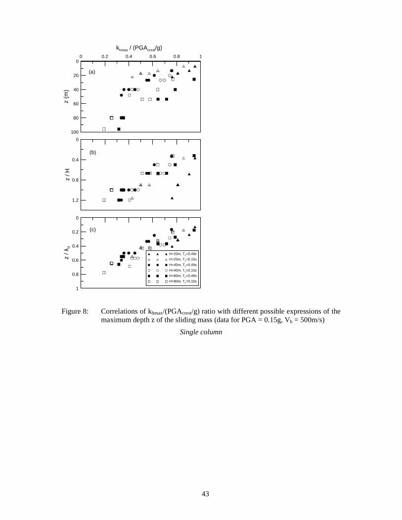
43

Figure 8: Correlations of khmax/(PGAcrest/g) ratio with different possible expressions of the maximum depth z of the sliding mass (data for PGA = 0.15g, Vb = 500m/s)

Single column

0 0.2 0.4 0.6 0.8 1

khmax / (PGAcrest/g)

100

80

60

40

20

0z

(m)

1.2

0.8

0.4

0

z / H

1

0.8

0.6

0.4

0.2

0

z / λ

d

H=20m, Te=0.49s

H=20m, Te=0.15s

H=40m, Te=0.49s

H=40m, Te=0.15s

H=80m, Te=0.49s

H=80m, Te=0.15s

(a)

(b)

(c)

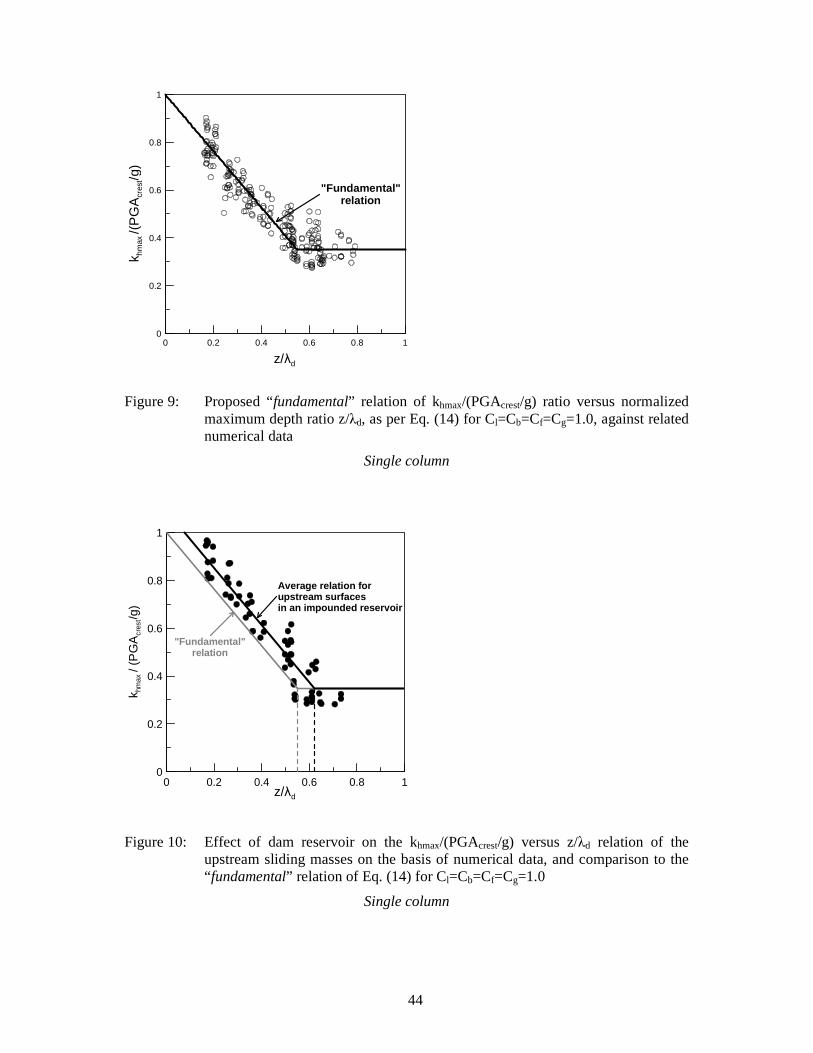
44

Figure 9: Proposed “fundamental” relation of khmax/(PGAcrest/g) ratio versus normalized maximum depth ratio z/λd, as per Eq. (14) for Cl=Cb=Cf=Cg=1.0, against related numerical data

Single column

Figure 10: Effect of dam reservoir on the khmax/(PGAcrest/g) versus z/λd relation of the upstream sliding masses on the basis of numerical data, and comparison to the “ fundamental” relation of Eq. (14) for Cl=Cb=Cf=Cg=1.0

Single column

0 0.2 0.4 0.6 0.8 1

z/λd

0

0.2

0.4

0.6

0.8

1

k hm

ax /(

PG

Acr

est/g

)

"Fundamental"relation

0 0.2 0.4 0.6 0.8 1z/λd

0

0.2

0.4

0.6

0.8

1

k hm

ax /

(PG

Acr

est/g

)

"Fundamental"relation

Average relation for upstream surfaces in an impounded reservoir

45

Figure 11: Prediction accuracy of the peak seismic coefficient khmax for sliding masses, against all numerical data

Single column

Figure 12: Effects of important problem parameters To/Te, z/λd and PGA on the relative error of khmax prediction for all numerical data

Single column

0.01 0.1 10.02 0.05 0.2 0.5 2khmax from analyses

0.01

0.1

1

0.02

0.05

0.2

0.5

2

pred

icte

d k

hmax

Η = 20mH = 40mH = 80mH = 120m

accuracy of +27%

0 2 4 61 3 5 7To / Te

-0.8

0

0.8

1.6

R_k

hmax

0 0.2 0.4 0.6 0.8 1z / λd

-0.8

0

0.8

1.6

R_k

hmax

0 0.2 0.4 0.6PGA (g)

-0.8

0

0.8

1.6

R_k

hmax

H = 20mH = 40mH = 80mH = 120m

(a)

(b)

(c)

46

Figure 13: Permanent deviatoric slope displacements D as a function of ky, PGA and PGV from various upper bound (UB) and average (AVE) relations based on the rigid sliding block theory

Single column

Figure 14: Correlation of sliding coefficient q to allowable displacement Dall and peak seismic intensity measures of the sliding mass khmax and vhmax on the basis of upper bound (qUB) and average (qAVE) displacement equations

Single column

0.1 10.2 0.5 20.05

ky / (PGA/g)

0.1

1

10

100

1000

D /

[PG

V2 /

PG

A]

UB: Richards & Elms (1979)UB: Cai & Bathurst (1996)UB: Newmark (1965) ky/(PGA/g) > 0.16

UB: Newmark (1965) ky/(PGA/g) < 0.16

AVE: Whitman & Liao (1984)PROPOSED equation (UB)

Range of predictionsFranklin & Chang (1977)

0.01 0.1 1 100.03 0.3 3 30

Dall / [vhmax2/(khmaxg)]

2

4

6

8

10

1

3

5

7

9

slid

ing

fact

or q

(=k

hmax

/khE

)

qAVE

qUB

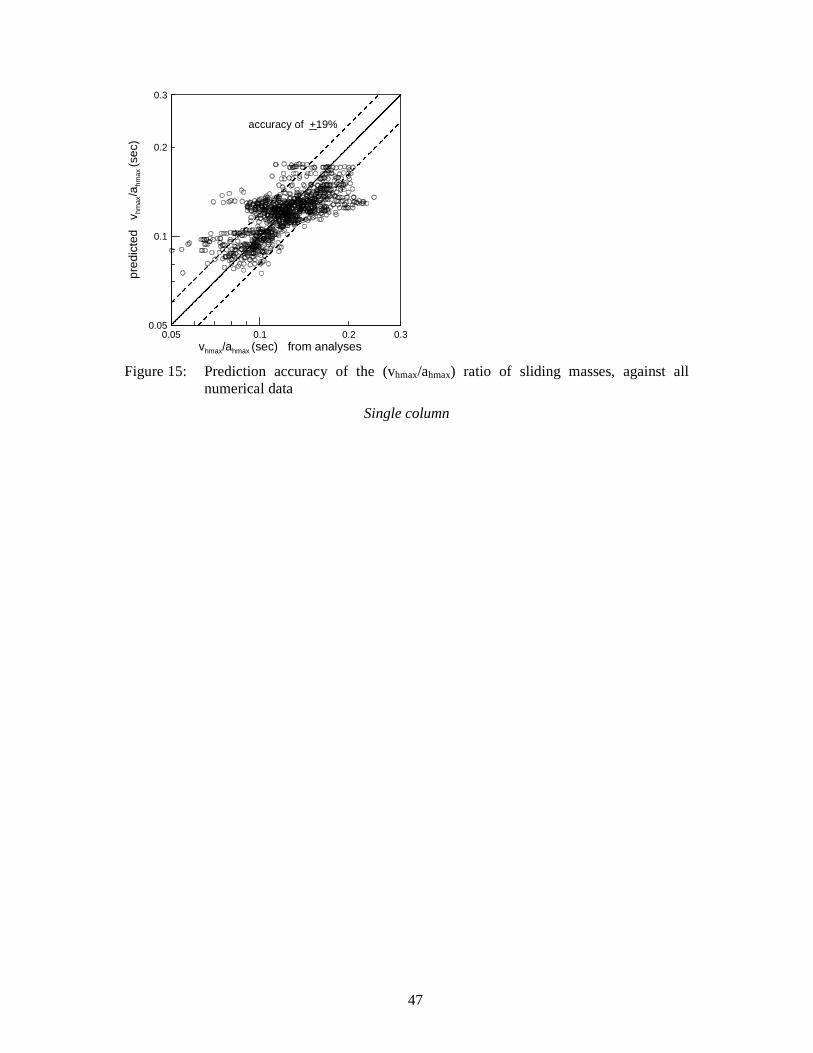
47

Figure 15: Prediction accuracy of the (vhmax/ahmax) ratio of sliding masses, against all numerical data

Single column

0.1 0.2 0.30.05vhmax/ahmax (sec) from analyses

0.1

0.2

0.3

0.05

pred

icte

d v

hmax

/ahm

ax (s

ec)

accuracy of +19%