Appendix A Estimating the AR Coefficients for the 3DAR Model

This appendix presents the least squared solution (the Maximum Likelihood solution may be found in [149]) for the coefficients of the three dimensional autoregressive model as outlined in Chapter 2. The model is best discussed in its prediction mode. The prediction equation is as below where i ( i, j, n) is the predicted value of the pixel at ( i, j, n).

N

I(i, j, n) = L ak!(i + qk(x) + SXn,n+qk(n), j + qk(y) + SYn,n+qk(n), n + qk(n)) k=l (A.1)

The task then becomes to choose the parameters in order to minimize some function of the error, or residual,

t:(i,j,n) = I(i,j,n)- I(i,j,n) (A.2)

The parameters of the model are both the AR coefficients a= [a 1 ,a2 ,a3 .. aN], and the displacement dk,l = [sxk,l SYk,l OJ. This section is concerned only with coefficient estimation given an estimate for the displacement.

The coefficients are chosen to minimize the squared error, ;:(), above. This leads to the Normal equations [11, 32, 71]. The derivation is the same as the one dimensional case and the solution can be determined by invoking the prin­ciple of orthogonality. E[t:2 (i,j,n)] is minimized by making the error t:(i,j,n) orthogonal to the signal values used in its generation [71]. Therefore,

E[t:(i, j, n)I(i + qm (x) + SXn,n+qm(n), j + qm(Y) + SYn,n+qm(n)' n + qm(n))]

= 0 (A.3)

274 Appendix A. Estimating the AR Coefficients for the 3DAR Model

Where m = 1 ... N. Defining q0 = [0, 0, OJ and a0 = 1.0, then

N

E(i, j, n) = 2:.>kl(i + qk (x) + SXn,n+qk(n), j + qk(y) + SYn,n+qk(n), n + qk(n)) k=O (A.4)

Note that the ak are now reversed in sign to allow for this simpler formulation. To continue, the following notation is introduced.

X [i j nJ [qk(x) qk(y) qk(n)J

[sxn,n+qk(n) SYn,n+qk(n) OJ

Substituting for E() in equation A.3 gives,

N

L akE[I(x + qk + dx,x+qk)I(x + qm + dx,x+q,JJ k=O

0

Vm l..N

(A.5)

(A.6)

(A.7)

(A.8)

The expectation can be recognized as a term from the autocorrelation function of the 3-D signal J(x). Matters may be simplified therefore by redefining the equation as

N

LakC(q~,q;,_,) = 0 (A.9) k=O

Where q~, q;,_, are both motion compensated vector offsets as defined impli­citly in the previous equation. However, a0 has already been defined to be 1.0. Therefore, letting

a = [at a2 .. aNf

c

c

C(q~' q~) C(q;, qD C( q~, q1')

C(q~,q;) C(q;,q;) C(q~,q;)

C(q~' q~) C(q;,qN) C(q~, q~v)

c ( qN, q~) c ( qN, q~) c ( qN, qN l [ C ( qo , q~ ) C ( qo , q;) ... C ( qo , qN) J

[0 0 0]

the parameters, a can be determined by solving

Ca= -c

(A.lO)

(A.ll)

(A.l2)

(A.l3)

(A.l4)

It must be pointed out that although C is symmetric, it is not Toeplitz in the multidimensional case. This is due to the fact that along a diagonal, the differences between the offset vectors that define each correlation term are not

Appendix A. Estimating the AR Coefficients for the 3DAR Model 275

necessarily parallel or the same magnitude. Consider the diagonal of matrix C, consisting of terms at locations (2, 1](3, 2](4, 3] ... [N, N -1], where the top left element of Cis at position (1, 1]. Then vector v~ = [q~- qU is not necessarily equal to v2 = [q~- q~] or v3 = [q~- q~] or any other such difference vector along the diagonal. The support vectors q may be chosen to allow this to occur by choosing vectors that lie along a line in the support volume. In general, however, when the support set delineates some volume, the vectors do not allow C to be Toeplitz. Therefore, it is difficult to exploit the structure of this matrix for computational purposes.

In the book, the equation A.14 is solved exactly. That is to say that no approximations about the autocorrelation function are made in estimating C or c. The expectation operator in equation A.9 is taken to be the mean operation. Note that in order to calculate the required autocorrelation terms from a block of data of size N x N in the current frame n say, the offset vectors q require that data outside this block is necessary. The extent of this extra data is explained next.

Figure 2.5 shows a support set of 5 vectors. Calculation of C(qo, q2), say, requires the following sum of products, where q2 = (-1, 0, -1].

L I(x + qo)I(x + q2 )

xEB1

(A.15)

Block B1 is of size N x N as stated before, and this yields data for I(x + qo). The term I(x + q2) requires data from a block, B2, which is in the previous frame and the same size, but offset by q2 in that frame. In this case therefore, to solve for the AR coefficients exactly in blocks of size N x N involves data from a block of size (N + 2) x (N + 2) in the previous frame centred at the same position.

Appendix B The Residual from a Non-Causal AR Model is not White

This section investigates the nature of the residual sequence from an AR model given a least squared estimate for the coefficients of the model. The analysis shows that unlike the causal AR model, the error or residual sequence of a non­causal model is not white but coloured (See [71, 149, 193, 192]). The model is considered in its 3D form as introduced in Chapter 2.

The model equation is as follows (see Chapter 2).

N

I(x) = ~ akl(x + qk) + c:(x) (B.1) k=l

This form of the model does not allow for any motion of objects between frames. Incorporation of this movement makes the expressions more cumbersome but does not affect the result. Typical support sets of N = 9 and N = 1 vectors defined by different qk are shown in Figure 3.8.

In solving for the coefficients using the least squared approach (see Ap­pendix A), the error, c:(x) is made orthogonal to the data at the locations pointed to by the support vectors, qk. This implies that

E[c:(x)I(x + qn)] = 0 for n = 1 ... N (B.2)

The goal of this analysis is to find an expression for the correlation function of c:(x). That is

R .. (x, qn) = E[c:(x)t:(x + qn)] (B.3)

Multiplying equation B.1 by c(x + qn) and taking expectations gives

N

E(I(x)c(x + qn)] = ~ akE[I(x + qk)E(x + qn)] + E[c(x)t:(x + qn)] k=l (B.4)

278 Appendix B. The Residual from a Non-Causal AR Model is not White

Let the variance of E(x) be (J;c Then from B.4, when qn = [0 0 0],

E[J(x)t:(x)] = a;, (B.5)

The summation term disappears because of equation B.2, since x :j:. (x + qk)·

When the qn refer to other positions within the support of the model then the following simplifications may be made

E[J(x)t:(x + qn)] 0 by B.2 (B.6)

N

~ akE[I(x + qk)E(x + qn)] (B.7) k=l

These simplifications can be substituted into B.4 to give the correlation term for non-zero vector lags. From this substitution it can be seen that the correlation structure of t:(x) is not white and it depends on the model coefficients. The final result then is

for qn = [0 0 OJ for n = 1 ... N

(B.S)

Appendix C Estimating Displacement 1n the 3DAR Model

The three dimensional autoregressive model incorporating motion is defined as below (from Chapter 2).

I(i,j,n)= N

I>kJ(i + qk(x) + SXn,n+qk(n), j + qk(y) + SYn,n+q, (n), n + qk (n)) + E(i, j, n) k=l (C.l)

The parameters of the model are both the AR coefficients a= [a1 , a2 , a3 .. aN], and the displacement dk,l = [sxk,l syk,l 0]. This section is concerned only with Least Squares displacement estimation given an estimate for the coefficients. For a Bayesian approach see Chapter 7.

In order to gain an explicit relation for E( ·), in terms of d, the approach used by Biemond [17] and Efstratiadis [37], was to expand the image function, I(-), in the previous frames, as a Taylor series about the current displacement guess. This effectively linearizes the equation for E(-) and allows a closed form estimate for d. It is this solution that is used for estimating d in this work. The derivation given here is for a general non-causal model which involves support in both the past and future frames as well as the current frame.

It is necessary first of all to separate the support region for the AR model into three parts.

1. The support in the frames previous to the current one, i.e. qk ( n) < 0. This is the temporally causal support.

2. The support in the current frame, qk(n) = 0.

3. The support in the frames to come, qk ( n) > 0. The temporally anti-causal support.

280 Appendix C. Estimating Displacement in the 3DAR Model

Further, given the displacement dz,ZH from frame l to frame l + 1 and d1,1_ 1

defined similarly, the displacement dl,l+k is defined as the linear sum of the displacements from frame l through to frame l + k. That is

Similarly for dz,l-k·

k-1

dz,l+k = d!,!+1 + L dm,m+l

m=!+1

(C.2)

The notation for the modelling equations is now improved slightly to allow a more condensed derivation of the estimation equations.

• qk(f) is the spatial support vector in the (n+f)th frame

• n is the current frame

• x is a spatial position vector

• I ( x, n) is the grey level at the position x in the nth frame

• N(f) is the number of points in the support of the 3D AR model in frame n +f.

• N0 is the number of points in the support of the 3D AR model in the current frame.

• F- is the maximum frame offset in the causal support (a negative number for the number of causal frames)

• F+ is the maximum frame offset in the anti causal support (a positive number for the number of anti causal frames)

• a- the coefficients for the temporally causal support

• a the coefficients for the support in the current frame

• a+ the coefficients for the temporally anti-causal support

The modelling equation can now be broken up into

I(x, n) No

L akf(x + qkJ n) k=O

p- N(f)

+ L La;; I(x + qk(f) + dn,n+f, n +f) f=-1 k=1

p+ N(f)

+ L L at I(x + qk(f) + dn,n+f, n +f) !=1 k=1

+ c(x, n) (C.3)

Appendix C. Estimating Displac€ment in the 3DAR Model 281

If the various support is then expressed in terms of the displacement into the next and previous frames, the following equation results after using C.2.

No

I(x, n) I.>kl(x + qb n) k=O

p- N(f) n+ /+1

+ L La; I(x + qk(f) + dn,n-1 + L dm,m-1 1 n +f) /=-1 k=l m=n-1

p+ N(f) · n+f-1

+ L L at I(x + qk(J) + dn,n+l + L dm,m+l: n +f) /=1 k=l m=n+l

+ t:(x, n) (C.4)

It is assumed that there exist already estimates for dn,n+l and dn,n-l· What is required is therefore an update for each value. Let the current estimates be d~,n+l and d~,n-l· Further, let the updates required be such that

dn,n+l = d~,n+l + Un,n+l

dn,n-1 d~,n-1 + Un,n-1

Where u represents the update to be found. Equation C.4 can now be written as

No

I(x, n) L aki(x + qb n) k=O

p- N(f) n+ f+l

(C.5)

(C.6)

+ L La; I(x + qk(f) + d~,n-1 + Un,n-1 + L dm,m-l,n +f) /=-1 k=l m=n-1

p+ N(f) n+f-1

+ L L at I(x + qk(f) + d~,n+l + Un,n+l + L dm,m+l: n +f) /=1 k=l m=n+l

+t:(x,n) (C.7)

The function for I(·) given in equation C.7 can then be linearized using a Taylor expansion1 about (x + qk(f) + d~,n+l + l:dm,m+l,n +f), which represents the current displacement in both previous and next frames2 . The form of the next expression is unwieldy unless the following definition is made.

(C.8)

1 Note that this is not the only expansion that can be employed, an alternative is to use a Bilinear interpolation function. However, the first order Taylor expansion gives a simpler solution.

2The limits on the summation of displacement vectors are intentionally left out to allow the same expression to be used for the forward and backward displacement depending on the equation context.

282 Appendix C. Estimating Displacement in the 3DAR Model

The Taylor series expansion then yields the following expression.

I(x,n) No

I>ki(x + Qk,n) k=O

F- N(f)

+ L L a/J(D(J, k, n), n +f) J=-1 k=1

r N(f)

+ u~,n-1 L L aJ;VI(D(f,k,n),n+f) f=-1 k=1

r N(f)

+ L L aJ;v(D(j,k,n),n+f) J=-1 k=1

F+ N(f)

+ L L ati(D(j,k,n),n+f) /=1 k=1

F+ N(f)

+ L L atv(D(f,k,n),n +f) /=1 k=1

F+ N(f)

+ u~,n+ 1 L L atV I(D(J, k, n), n +f) /=1 k=1

+ c(x,n)

v(·) represents the higher order terms in the Taylor series expansions.

(C.9)

For the current set of estimated parameters, a and d 0 there will be some observed error Eo. This error is defined as (following A.l),

Eo(x, n) No

I(x, n) - L aki(x + Qkl n) k=O

r N(f)

L L aJ; I(D(f, k, n), n +f) f=-1 k=1

F+ N(f)

- L L ati(D(f,k,n),n +f) /=1 k=1

(C.lO)

Appendix C. Estimating Displacement in the 3DAR Model 283

Therefore substituting C.9, an expression involving u in terms of observables follows (where the limits on the sums have been dropped).

Eo(x, n) u~,n-l L L aJ;\l I(D(f, k, n), n +f)

+ LLaJ:v(D(f,k,n),n +f)

+ u~,n+l L La tV I(D(J, k, n), n +f)

+ LLatv(D(f,k,n),n+f)

+ t:(x, n) (C.ll)

The spatial, two component, update vectors, u are now required, but there is only one equation. Collecting observations of Eo (x, n), \l I(-) at each position in some predefined region, an overdetermined system of equations results. These equations can be written as follows:

( C.12)

The quantities are defined as follows, given a set of equations made by observing a block of N1 x N 2 pixels.

• zw, (N1 x N2 x 1) is a column vector of current errors at all the points in the region used for estimation.

Eo(Xt,n) Eo(x2, n)

(C.13)

• Gw, (N1 x N2 x 4) is a matrix of gradients at the past and future support positions.

"'"' - o!t(D(f,k,n)) L.. L.. ak ox "'"' - o!,(D(f,k,n)) L.. L.. ak ox

"'"' - o!t(D(f,k,n)) L.. L.. ak oy "'"' - oi2(D(f,k,n)) L.. L.. ak oy

(C.14)

• u is the ( 4 x 1) vector of updates defined as

u = [ ~:::~~ ] (C.15)

284 Appendix C. Estimating Displacement in the 3DAR Model

• v w is the collection of all the error terms E and v.

l L:L:a;vl( ... )+L:L:atvl( ... )+c(xl,n) l L L a;v2( ... ) + L L atv2( ... ) + c(x2, n)

Vw = ~ L a;v(NrN2) (. · ·) + L L atv(NrN2) (. · ·) + E(X(NrN2)' n)

So far the derivation for the parameter estimates has placed no restriction on the spatial or temporal nature of the model support. However, the work in the book is concerned with causal modelling primarily due to the decreased computation necessary.

Solving for the updates.

It is possible to estimate the displacement update vector in C .12 directly via the pseudo inverse of Gw as follows:

G~Gwu+G~vw [G~Gw]- 1 [G~zw- G~vw] (C.l6)

To arrive at a more robust solution, the approach adopted by [37] has been to derive a Wiener estimate for u [37, 17]. The method was initially presented by Biemond, and it attempts to find the estimate u for u which minimizes the error E[[u- u[ 2 ]. Therefore,

E[(uT- u.T)(u- u)] E[uT u- UT u- u.T u + u.T u] (C.l7)

The estimate, u, is found from a linear transformation of the observed error vector z such that

u = Lzw (C.l8)

Substituting this expression for u in C.l7 and differentiating with respect to the required unknown, L, to find the minimum squared error, yields the following equation.

LE[(Gwu + v)(Gwu + vwf] = E[u(Gwu + vwf] (C.l9)

Therefore, assuming that, v w, which involves higher order terms, is uncorrel­ated with the actual update, u, an explicit expression for L results.

(C.20)

This solution for L involves the inverse of a large matrix. If the number of positions at which observations are taken is P, then it involves the inverse of a P 2 x P 2 matrix. Biemond [17] has employed a matrix identity which simplifies this solution considerably.

RuuG~[GwRuuG~ + Rvvr 1 = [G~R;v1 Gw + R~~r 1 G~R;v1

(C.21)

C.l Summary 285

Using C.21, therefore,

(C.22)

Assuming that the vector v represents white noise and that the components of

u are uncorrelated, i.e. Rvv = O"~vi and Ruu = O"~ui, L is given by

(C.23)

2

where f..L = ~- Due to the identity in C.21 and this assumption, the matrix ""uu

inverse is reduced to the inverse of a 2 x 2 matrix , regardless of the number of equations.

It is important to recognize that the validity of the assumption regarding Rvv is affected by the causality of the model support. This is because part of v consists of the model error t:(·). It has been shown in [107, 192, 193, 71], that this error is not white when the model support is non-causal. This implies that if the support for the model consists of points in the current frame that represent a non-causal region in that frame, the assumption is not valid. To ensure the validity of the white noise assumption, the support for the AR model in the current frame must be limited to a causal region, i.e. to the left and above the predicted location.

The Wiener estimate for u is therefore given by

(C.24)

This solution for the update for the current displacement is incorporated into an iterative refinement scheme. A guess for the displacement, which may be zero, is iteratively refined using the above equation until some convergence criterion is satisfied. Two main criterion are used in this book, a threshold on the magnitude of the error vector, lzw It and a threshold on the size of the update vector, lult- The iterative refinement process is halted if the magnitude of the current error is less than lzw It or the magnitude of the update is less than lult· A final criterion is the most harsh, and simply halts iteration if no other criterion has been fulfilled when a certain number of iterations have completed. These criterion are necessary to limit the computational load of the algorithm.

C.l Summary

The approach taken by Biemond [17] can be used to generate a solution for the motion update in the case of the general 3DAR model. The solution is linear only if the model coefficients are known beforehand. These are not available in practice but it is possible to estimate the coefficients and displacement success­ively in the iterative process. The motion equations reduce to approximately the same form as the standard WBME.

It is important to recognize that the Taylor series expansion is not the only expansion which can be used to linearize the model equation. The purpose of

286 Appendix C. Estimating Displacement in the 3DAR Model

the expansion is to make the displacement parameter available explicitly. To this end any interpolator would suffice. The compromise is one of interpolator quality versus computation. Sine interpolation is a possibility but it would yield a non-linear solution. Bilinear interpolation is also an alternative which may prove better than the Taylor expansion. This book uses the Taylor expansion to facilitate a simple linear solution but other interpolators would be useful to consider in further work.

Appendix D Joint Sampling in the JOMBADI Algorithm

This Appendix presents the details for the derivation of the various conditional distributions required for the JOMBADI algorithm. The discussion begins with a restatement of the basic models as follows:

The observation model is Gn(x) = (1- b(x))In(x) + b(x)c(x) (D.l)

p

The (clean) image model is In(x) = :2:: akfn+q~ (x + q%) + e(x) k=1 (D.2)

where all the required data is compensated for motion, Gn is the nth degraded frame and In is the nth original, clean frame. The parameters to be estimated are b(x) (set to 1 when site x is corrupted and zero otherwise), the P 3DAR model coefficients a (a0 = 1.0), the clean original data In(x) at sites where b(x) = 1, and the motion vector fields dn,n-1 , dn,n+l· The motion information is left out of the image model for simplicity. The parameter vector containing all the variables is denoted e. When it is required to define a parameter vector which contains a subset of the parameters, this vector is denoted e-(a,u~) for instance, for a subset which does not contain the 3DAR model parameters. There are two main sampling steps, sampling jointly for b(x), c(x), I(x) and sampling jointly for a, O"~, dn,n-1 , dn,n+l· The latter sampling strategy is more straightforward to derive and it is considered first.

288 Appendix D. Joint Sampling in the JOMBADI Algorithm

D.l Sampling for a(x), O';(x), dn,n-I(x)

Recall that the 3DAR model parameters and motion vectors are block based. In this section although x is the position vector of a particular site in a frame, the values for a, 0';, dn,n-1 (x), dn,n+1 (x) are the same over each B x B block of pixels in the image. This section drops the x argument for the various block based parameters to keep the notation simple. Consider a single block of pixels. The joint sample required is drawn from the distribution

p(a, (]';, dn,n-1lln, In-1, In+l, dn,n+l, D) (D.3)

in which D denotes the block based motion vector neighbourhood around the current block position. Raster scanning all the necessary image data into the column vector i, this distribution may be decomposed as follows:

p(a,CJ';,dn,n-1li,dn,n+1,D) =

p( ai(]';, dn,n-1, i, dn,n+l, D)p( (]'; idn,n-1, i, dn,n+1, D)p( dn,n-1ii, dn,n+1, D) (D.4)

The first conditional distribution on the right hand side results from

( I 2 d · d D)_ p(a,CJ';,dn,n-1,i,dn,n+1,D) p aO'e, n,n-1,1, n,n+1, - J ( 2 d • d D)d

p a,CJ'e, n,n-1,1, n,n+1, a (D.5)

The joint distribution in the numerator of the expression above is the joint posterior distribution in equation 7.4. To avoid some unnecessary algebraic manipulation, the following analysis is useful.

Suppose the conditional p(aib) is required, where a and bare some random variables. Proceeding in the usual way,

p(aib)

=

p(a, b)

p(b) p(a, b)

fap(a,b)da (D.6)

The denominator is independent of a and is just a normalizing term which ensures the derived expression, p(aib), integrates to 1, if b is treated as a given constant. This extremely important result shows that to derive the conditional distribution for a random variable given the joint distribution, it is only neces­sary to collect together the terms which involve that particular random variable, and then derive the normalizing constant (if required). This rearrangement may not be straightforward in some cases, but fortunately, in equation 7.4, the only term which involves a is the image likelihood and this is a multivariate Gaus­sian. This makes it simple to perform the necessary manipulations.

Returning then to the original problem of deriving the conditional for a, note that the prediction error e in a volume of data including the current block of pixels can be written as e = i- Ia. The image data is scanned into the matrix I

D.l Sampling for a(x), u;(x), dn,,.-1 (x) 289

so that Ia is the prediction of a pixel at a particular site in the volume. e, i are column vectors that are B 2 elements long and the image data in I may need to come from outside the current block to provide the necessary support for the prediction required. Since each element of e is drawn from N(O, a;), and the only term involving a is the likelihood,

2 • 1 ( [i- IajT[i- Ia]) p(a,ue,dn,n-I,I,dn,n-l,D) ex J2t7Iexp - 2a;

(D.7)

where the proportionality symbol ex indicates thaf there are other terms which do not involve a, such as the priors p(dn,n-IID)p(a;). As explained before, these terms are not important for the conditional p( al ... ) .

This expression can be rearranged by completing the square in the argument of the exponent as follows:

[i- Ia]T[i- Ia] = iTi- 2iTIT a+ aTilT a

=(a- (IITt1Iif(IIT](a- (Iet1Ii]

+ iTi- iTIT(IITtlli (D.8)

Again ignoring the terms which do not involve a, the argument of the exponent can be seen to have the form of a multivariate Gaussian and so the conditional may be written as

This results in the expression as required (framed for emphasis):

2

p(aiB-a, i, D) "'N(a, ~) (D.9)

where a= [IIT]- 1 Ii is the least squares estimate for the P 3DAR coefficients, and the matrices liT and Ii can be recognized as the required covariance matrix and vector as described in Appendix A. Note that the multivariate distribution is of dimension P, the order of the 3DAR model, hence the variance term in the normalizing factor is raised to this power, not N, the number of pixel sites used for prediction error equations in the motion compensated data volume.

To derive the conditional p(u;IB-(a,<T~),i), the coefficients need to be integ­rated out of the posterior since

( 2!B . ) p(B-a,i,D) p O"e -(a,<T~), I, D = r (B . D)d 2

J<T;P -a,I, O"e

where

(D.lO)

290 Appendix D. Joint Sampling in the JOMBADI Algorithm

Having already completed the square to find the conditional for a the integra­tion of the posterior is made simpler by the important observation that

1 IKI! ( [x- xjTK[x- :X]) P exp - 2 2 dx = 1

x V2Jru2 CJ

(D.ll)

for a general multivariate Gaussian distribution N(x, 1~ 1 ), in which xis of di­

mension P. See [172] for some basic information about the multivariate Gaus-sian.

The analysis can now proceed as follows:

1 p(B-a, i, D)da ex

1 1 ( [a- [IITJ- 1 IijT[IIT][a- [IITJ- 1 li]) exp - da

(2Jru2) N /2 2u2 e a e

(D.12)

In the final expression above, the reader is reminded that the motion vec­tors dn,n- 1 , dn,n+l are implicit arguments to all the image data since they are needed to compensate for motion. There is only one other term in the posterior which involves u; and that is the prior p(u;). As stated earlier, this prior is suitably non-informative: p(u;) ex 1/u;. The derivation of the required condi­tional is similar to that presented in [151]. Note that if a= a in equation D.8 above, then it is easy to rewrite the last term in equation D.12 as follows in the conditional.

2 • p(u~) ( ere) p(ue!B-(a,,.~),I) ex N-P exp -22

fiiW'J (Je

where e = i- Ia

substituting for the prior, (D.13)

1 ( ere) ex '1-P exp --?

u~~, 2ue

The Inverted Gamma distribution [14] with parameters a, (3 is defined as

IG(x!a, ,8) = ~:) x-(et+l) exp-(!3/x) (D.14)

D.2 Sampling for b(x), c(x), In(x) 291

Comparing this with the expression for p( u; I ... ) results in the required ex­pression as follows (setting x = u;):

(D.l5)

The final conditional required is the conditional for the motion given the image data. This is derived by integrating out the variance from the expres­sion D.l2 for the same reasons as previously stated in deriving the conditional for the variance. Recall that the motion is an implicit variable in the assembly of the image data i, I (and of course in e). Because the motion is involved in the data I the factor outside the exponential cannot be ignored. The integration can be performed by using equation D.l4 and J IG(xla, (3)dx = 1 to yield

Therefore

(D.16)

where p( dn,n-1 ID) is the prior for motion, given the block based motion neigh­bourhood. A similar situation exists for p(dn,n+1 ID, i) and the relevant expres­sion can be part of a separate joint sampling step for motion in this direction.

D.2 Sampling for b(x), c(x), In(x)

The derivation of this joint sample is somewhat unusual because the observed data likelihood is a delta function. In fact this makes the required integration steps quite simple, but it is unlikely that the reader would have previously encountered the manipulation of distributions like these in this context. As with the derivation of the previous joint sampling strategy, the heart of the analysis is the successive integration of two of the three variables out of the joint posterior. The order in which this integration is done does affect the complexity of the resulting expressions, although it does not affect the computational complexity of the final algorithm. Recall that these sampling steps are performed on the pixel grid. In the discussion which follows, in(x), 9n(x) refer to the value of a pixel at site x in the original, clean image frame n and the dirty observed frame n, respectively. Similarly b(x), c(x) refer to the values of the detection field and corruption field at site x, respectively. To indicate that data has been compensated for motion, the superscript m is used. Thus I~_ 1 is shorthand for motion compensated data in frame n-1. The notation e-(b,i,c) is used to refer to the parameter vector without the variables b(x), i(x), c(x). The sampling order

292 Appendix D. Joint Sampling in the JOMBADI Algorithm

adopted is b(x) followed by in(x) then c(x). These steps require integrating out c(x) then in(x) in that order. The joint posterior can be written

p(b(x), in(x), c(x)lgn(x), 1:_1 , 1:+1, B, C, B-b,-i,-c) ex

p(gn(x)IB, 1:_1, 1:+1, B, C)

X Pi(in(x) IB-b,-c, 1:_1, 1:+1, B, C) Pc(c(x)IC) Pb(b(x) I B) (D.17)

where B, C refer to the current values of the 8 connected neighbourhood around the site x in the detection and corruption fields.

Each term in the posterior is as below

p(gn(x)IB, ... ) = 6(gn(x)- (1- b(x))in(x)- b(x)c(x))

= {6(gn(x)- in(x)) for b(x) = 0 (D.1S) 6(gn(x)- c(x)) for b(x) = 1

. I a~ au I~ ( 1 . o T . o ) p;(2n(x)IB-(b,c)> ... ) = ~ exp --2 2 [2n(x)- t](auau)[2n(x)- 2] y 21w; CJe

' (J2

=N(i,-:/-) au au

, aT Akik where i = _u"-:y=--­

auau

Pc(c(x)IC) ex exp (- L A~(l- u(z, x))lc(x)- zl) zEC

Pb(b(x)IB) ex exp (-~ .\~(1- u(z, x))lb(x)- zl)

(D.19)

(D.20)

(D.21)

The expressions D.20 and D.21 are both taken from their original definitions found in equations 7.9, 7.10. The expression for the conditional for in(x) is derived following the same arguments that led to equation 7.35, except consid­ering one missing pixel only, in(x) in this case. Therefore au is now a column vector as opposed to a matrix. Further details about the composition of Ak etc. can be found in the discussion on fast algorithms in section 7.8 of Chapter 7. The manipulations required to yield the final form of equation D.19 are the same as those leading up to equation D.9 in this appendix.

Integrating out c(x) from the posterior yields

1 p(b(x), in(x), c(x)IB-(b,i,c)), ... ) dc(x) =

{p,(~n(x)~-b,-c, ... )Pc(c(x)=gn(x)~)Pb(b(x)=1IB) p;(2n(X)-gn(x)IB-b,-c, ... )pb(b(x)-OIB)

for b(x) = 1

for b(x) = 0 (D.22)

D.2 Sampling for b(x), c(x), In(x) 293

because

p,(in(x)=gn(x)JB-(b,c)• · · ·) (D.23)

8(gn(x)- c(x))Pc(c(x)JC) Pc(c(x)=gn(x) JC) (D.24)

Integrating i 11 (x) out of the expression for b(x) = 1 yields

1 [p;(in(x)JB-b,-c, ... )Pc(c(x)=gn(x)JC)pb(b(x)=1JB)] din(x) = ln (x)

Pc(c(x)=gn(x) IC)pb(b(x)=1JB) (D.25)

because, by definition

(D.26)

Integrating in(x) out of the expression for b(x) = 0 yields

1 [p,(in(x)=gn(x)JB-(b,c)• ... )Pb(b(x)=OJB)] din(x) ln (x)

p;(in(x)=gn(x)J ... )pb(b(x)=OJB) (D.27)

because,

Therefore the required conditional p(b(x)JB, ... ) is

(D.29)

where x has been omitted for brevity. This equation can be used to generate

the required sample for the binary b(x). Note that drawing a sample for b(x) requires knowledge of the normalizing constants for the distribution Pc ( c(x) JC) and p;(in(x)J ... ).

The form of the conditional for i 11 (x) can be seen to be

p(in(x)Jb(x), ... ) = {N(i, af:u) for b(x) = 1 8(g11 (x)- in(x)) for b(x) = 0 (D.30)

The delta function simply means that when b(x) = 0 there is no corruption

and so the underlying clean image is the observed image. Otherwise some in­

terpolation needs to be done and the image is interpolated using a sample from

the normal distribution as specified.

294 Appendix D. Joint Sampling in the JOMBADI Algorithm

Similarly, the form of the conditional for c(x) can be seen to be

( ( )I ( ) . ( ) ) = {6(gn(x)- in(x)) for b(x) = 1 p C X b X , 2n X , ...

Pc(c(x)IC) for b(x) = 0 (D.31)

with delta function meaning that when b(x) = 1 there is corruption and so the corruption field is the observed image. Otherwise the corruption field is a sample from the prior alone.

Sampling for the data in this order makes the samples for in(x) and c(x) easy to generate since b(x) is already sampled first.

Appendix E Examining Ill~Conditioning 1n GTG

Several workers1 all recognized that when gradient based algorithms failed they did so primarily because of the ill-conditioning of the Gradient matrix that was set up. This ill-conditioning can be quantified through the eigen values of the matrix. The analysis presented here considers this phenomerron and gives some basis for the final algorithm presented by Martinez [117] and reviewed in Chapter 2.

E.l Condition for singularity

In the standard WBME the solution for the update vector is given as

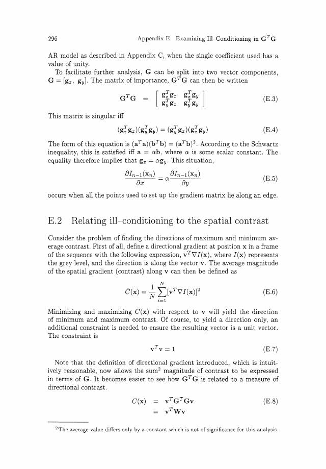
(see Chapter 2). The gradient matrix G contains elements as follows:

G I 8In-dxr) ax

81n-dx2) ax

~fn-1 (XN1 x N 2 )

ax

Bfn_J(xt) ay

Bin- t(x2) ay

8In_t(xN1 xN2 )

ay

(E.l)

(E.2)

Figure 2.3 illustrates the situation when solving for the motion update using

this technique. Note how this solution follows from using a one point temporal

1For instance, Martinez [117], Kearney eta!. [78] and Biiriiczky eta!. [20, 21, 35, 34].

296 Appendix E. Examining Ill-Conditioning in GTG

AR model as described in Appendix C, when the single coefficient used has a value of unity.

To facilitate further analysis, G can be split into two vector components, G = (gx, gy]· The matrix of importance, GTG can then be written

(E.3)

This matrix is singular iff

(E.4)

The form of this equation is (aTa)(bTb) = (aTb) 2 . According to the Schwartz inequality, this is satisfied iff a = ab, where a is some scalar constant. The equality therefore implies that gx = agy. This situation,

8In-dxn) 8In-l (xn) --~~~=a--~~~ ax ay (E.5)

occurs when all the points used to set up the gradient matrix lie along an edge.

E.2 Relating ill-conditioning to the spatial contrast

Consider the problem of finding the directions of maximum and minimum av­erage contrast. First of all, define a directional gradient at position x in a frame of the sequence with the following expression, vT\l I(x), where J(x) represents the grey level, and the direction is along the vector v. The average magnitude of the spatial gradient (contrast) along v can then be defined as

N - l"'T " C(x) = N L.)v \l I(x)]-

i=l

(E.6)

Minimizing and maximizing C(x) with respect to v will yield the direction of minimum and maximum contrast. Of course, to yield a direction only, an additional constraint is needed to ensure the resulting vector is a unit vector. The constraint is

(E.7)

Note that the definition of directional gradient introduced, which is intuit­ively reasonable, now allows the sum2 magnitude of contrast to be expressed in terms of G. It becomes easier to see how GTG is related to a measure of directional contrast.

C(x) (E.S)

2The average value differs only by a constant which is not of significance for this analysis.

E.2 Relating ill-conditioning to the spatial contrast 297

Another simplification is introduced, letting W = GTG. Combining equation E. 7 and E.9 and a Lagrange multiplier A., gives the

following expression to optimize.

O(.X., v) = vr[W- .X.I]v +A. (E.9)

Differentiating E.9 with respect to v and setting the result to zero, yields E.10.

[W - .X.I]v + [W - .X.If v = 0 (E.10)

But W is symmetric, therefore,

[W-.X.I]v = 0 (E.ll)

This is an eigenvalue problem. Therefore, the directions of maximum and min­imum contrast lie along the eigen vectors of W. Similarly, the magnitudes of maximum and minimum contrast are given by eigenvalues of W. The larger eigenvalue and corresponding vector refer to the magnitude and direction of maximum contrast.

When W is ill-conditioned, Amax » Amin· Hence GTG is ill-conditioned when the directions of averaged spatial gradient are not of equal importance; at an edge for instance.The solution for the motion estimate is therefore well conditioned when the image portion consists of two clearly defined gradient directions. A good example is at a corner [131, 125].

This agrees well with intuition. As discussed in Chapter 2, vertical motion at a vertical (step) edge cannot be estimated. In that case all the information in the vertical direction would be the same. Any vertical motion would yield no change in information. Horizontal motion would of course yield a change in information because of travel across the vertical step. Therefore this motion can be readily estimated. This phenomenon can be summed up by stating that the motion estimate is most accurate in the direction of maximum contrast. This observation would reflect itself in the ill-conditioning of W by giving meaning to only one of the two equations for motion in equation E.l when the equations are set up at an edge. This cannot be unraveled in the straightforward inverse operation required in equation E.l, the only clue is that the solution becomes ill-conditioned.

In the light of this analysis it seems natural to detect ill-conditioning in the usual way, by thresholding the eigenvalue ratio, then proceed to stabilize the solution using eigen analysis. This analysis can then yield a direction in which the motion estimation is more accurate. This is the solution that Martinez proposed, and his solution is repeated here.

d = if Amax » Amin

otherwise (E.l2)

Here, A. and e refer to the eigenvalues and eigenvectors of GTG, and a is a scalar variable introduced to simplify the form of the final solution.

298 Appendix E. Examining Ill-Conditioning in GT G

Note that in the work of Martinez [117], the solution was neither pel-recursive nor was any consideration given to the use of the regularizing J.L used in E.1.

E.3 Ill-conditioning in the general 3DAR solution.

Following a similar approach to that of Martinez, it is possible to examine the relation between the WBME and the general AR estimator with respect to conditioning of the solution.

Consider a temporally causal AR model in which the support region con­sists of points in the previous frame only, for example, AR9 in Figure 3.8 in Chapter 3. Then, using the definition of ew in equation 3.7, it is possible to express the general matrix in terms of gx and gy , defined above, as follows:

(E.13)

A is a matrix of AR coefficients that would weight the relevant gradient terms of g to yield the general form indicated by equation 3.7.

From E.13 e~ew can be expanded to

[ g'I'Ar Agx g~Ar Agx

The matrix is therefore singular when

(E.14)

(E.15)

As before, the Schwartz inequality may be applied to yield the condition for singularity as

(E.16)

Provided that A has an inverse, the condition for a singular weighted gradient matrix, e~ew, is the same as for the matrix ere, as discussed previously. Therefore, the general 3DAR solution for motion is also ill-conditioned at an edge in the image.

An eigen analysis would yield similar conclusions to that discussed previously. The weighting matrix, A would change the eigen values and vectors of the un-weighted matrix, ere. Nevertheless, in view of the similar conditions for singularity, it would appear that 3DAR solution is not any better conditioned in this respect. In practice however, it is noticed that the solution is better behaved, and this must be due to the noise reducing effect of the gradient weighting.

E.4 Summary

An eigen analysis of the simple gradient based motion solution has related ill­conditioning to the presence of an edge in the image. The eigen values and

E.4 Summary 299

vectors of GT G have been shown to represent the value and directions of max­imum and minimum contrast in the image. Hence, the ill-conditioned solution can be related to the contrast orientation in the image, a standard problem.

In this respect, the 3DAR solution carries no advantage. It is also singular at edges in the image. However, it uses a weighted gradient matrix and each term therefore represents a weighted combination of gradient observations in a small region. This results in a less noisy gradient observation and so the solution is more stable.

The eigen analysis of both GT G and G~ Gw can be used to propose a strategy when the solution is detected as ill-conditioned. This strategy is used to good effect in Chapter 3.

Appendix F The Wiener Filter for Image Sequence Restoration

The Wiener filter has been used frequently in the past as an effective method for noise and blur reduction in degraded signals. The form of the filter for image sequences is a direct extension of the 1-D result, however the limited amount of temporal information available implies different considerations in the implementation of the method. This Appendix makes explicit the various forms of the filter that can be used and in so doing lays the foundation for the ideas presented in appendix G. The theory presented here ignores motion between frames. Motion is considered in the main body of the text.

This book concerns itself with the problem of noise reduction in image se­quences, blur is not considered. The observed signal model is then

g(i,j,n) = I(i,j,n) +J)(i,j,n) (F.l)

where g(i,j,n) is the observed signal grey scale value at position (i,j) in the nth frame, I( i, j, n) is the actual non-degraded signal and 7)( i, j, n) the added white noise of variance () TJTJ.

F.l The 3D frequency domain/3D IIR Wiener filter

The Wiener filter attempts to produce the best estimate for I(i,j,n), de­noted i ( i, j, n). It does so by minimizing the expected squared error given by

E[(e(i,j, n)) 2] = E[(I(i,j, n)- i(i,j, n)) 2] (F.2)

This estimate may be achieved using either an IIR or FIR Wiener filter, which operates on the observed noisy signal. The following two expressions show re-

302 Appendix F. The Wiener Filter for Image Sequence Restoration

spectively IIR and FIR estimators.

i(i,j, n) L L L a(kr, k2, k3)g(i + kr,j + k2, n + k3) (F.3) k1 k2 k3

i(i,j,n) N1 N2 N3

2: 2: 2: a(kr, k2, k3)g(i + kr, j + k2, n + k3) (F.4) k1=-N1 k2=-N2 k3=-N3

In equation F.3 there are no limits on the summations, hence IIR, and in equation F.4 the filter mask (or support) is a symmetric volume around the filtered location of size (2N1 + 1) x (2N2 + 1) x (2N3 + 1).

Proceeding with the IIR filter leads here to a frequency domain expression for the Wiener filter. Using the principle of orthogonality to bypass some lines of differential algebra, E[(e( ... )) 2] is minimized if the error is made orthogonal to the data samples used in the estimate equation F .3.

Substituting for e(i,j,n) in equation F.5 gives

E[f(i, j, n)g(i + kr, j + k2, n + k3)] =

E[I(i,j,n)g(i+kr,j+k2,n+k3)] V kr,k2,k3 (F.6)

The filter coefficients are then chosen to satisfy the condition of equation F.6. Substituting for f(i, j, n) in F.6 yields,

L a(lr,l2,l3)E[g(i + lr,j + l2,n + l3)g(i + kr,j + k2,n + k3)] 11,12,13

The expectations can be recognized as terms from the autocorrelation and crosscorrelation sequences of the observed image sequence g(i,j,n) and the actual sequence I(i, j, n). The solution involves a separate equation for each coefficient, i.e. an infinite set of equations. However, using the 3D DFT gives a tractable result in terms of the power spectra concerned. From equation F .6 the following expressions result assuming stationary statistics.

LLLa(lr,l2,l3)R99 (l1- kr,l2- k2,l3- k3 )]

11 12 13

Taking Fourier transforms yields

A(wr, w2, w3)P99 (w1, w2, w3) = Pi9 (w1, w2, w3) (F.9)

The only unknown quantity here is the cross power spectrum Pig. However, using the original assumption of uncorrelated noise and image frames, implies

F.2 The 3D FIR Wiener filter

that

303

(F.IO)

(F.ll)

From these two equations, an expression for the 3D frequency domain Wiener filter, A(w1,w2,w3) is as follows.

A( ) _ P99 (w1,w2,w3)- PTJ'I(w1,w2,w3) W1,w2,W3 -

P99 (w1, w2, w3)

The estimated signal, i(i,j,n) is then given by the expression below.

i(i,j,n) = IDFT[A(w1,w2,w3)G(w1,w2,w3)]

(F.l2)

(F.l3)

The IDFT is the inverse 3D DFT, and G(w1,w2 ,w3) is the 3D DFT of the observed signal, g(i,j,n). The filter is therefore defined by the signal power spectrum and the noise variance.

Using the 3D DFT in this way makes the Wiener filter computationally at­tractive. However, in the temporal direction there are often not many frames involved. Therefore, the temporal Fourier component is less meaningful, hav­ing been derived from only a few samples. In the book, 3 frames are involved, hence the DFT in the temporal direction involves just 3 samples. More frames can be included but at the expense of stationarity since effects such as occlu­sion and uncovering are more likely to appear. The assumption of an infinite support volume is violated. This phenomenon is also applicable to the spatial components since the image is only stationary over small areas. Therefore, in a practical situation, the 3D IIR filter implemented in the frequency domain in this way, is no longer IIR since it operates on a finite volume of input data only and not on any past outputs.

The problem may be overcome by considering two further forms of the filter which allow for finite support. One form follows from the FIR filter expression in equation F.3, the other results from a matrix formulation of the filter.

F .2 The 3D FIR Wiener filter

The FIR filter result follows again by using the theorem of orthogonality. The expression F .4 for the filter is substituted into the error term in the orthogon­ality expression F .5 using equation F .2, except allowing for the finite support. This yields

L a(l1, l2, I3)E[g(i + l1, j + l2, n + l3)g(i + k1,j + k2, n + k3)] lthh

E[I(i,j,n)g(i + k1,j + k2,n + k3)] (F.14)

{ -N, < k1, 11 5o N1 for -N3 5o k2, 12 5o N2

-N3 5o k3, 13 '5,N3

304 Appendix F. The Wiener Filter for Image Sequence Restoration

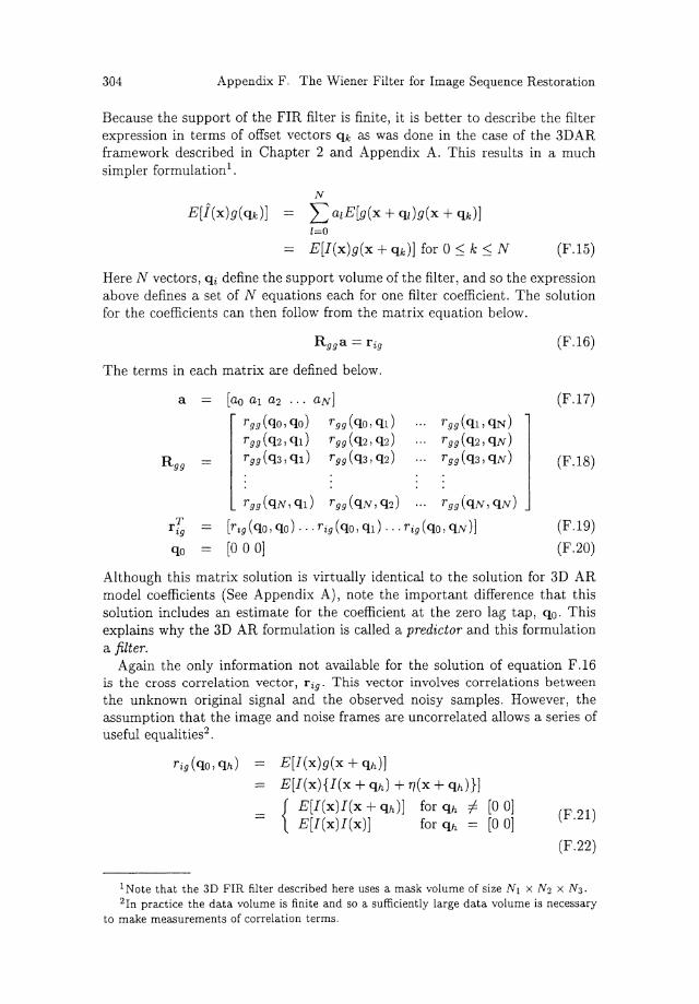
Because the support of the FIR filter is finite, it is better to describe the filter expression in terms of offset vectors Qk as was done in the case of the 3DAR framework described in Chapter 2 and Appendix A. This results in a much simpler formulation1.

N

E[i(x)g(qk)] = L atE[g(x + ql)g(x + qk)] l=O

E[I(x)g(x + qk)] for 0 ::::; k ::::; N (F.l5)

Here N vectors, Qi define the support volume of the filter, and so the expression above defines a set of N equations each for one filter coefficient. The solution for the coefficients can then follow from the matrix equation below.

The terms in each matrix are defined below.

a = [ao a1 a2 ... aN]

r99 (qo, Qo) r99 (qo, ql) r99 (q2,q1) r 99 (q2,Q2)

R r 99 (q3,qt) r 99 (q3,q2) gg

r99 (q1, QN)

rgg(Q2,QN) rgg(Q3, QN)

rg9 (qN, ql) rgg(QN, Q2) rgg(QN, QN)

[r,g ( Qo, qo) ... rig (qo, ql) ... rig (qo, QN )]

[0 0 OJ

(F.l6)

(F.l7)

(F.l8)

(F.l9)

(F.20)

Although this matrix solution is virtually identical to the solution for 3D AR model coefficients (See Appendix A), note the important difference that this solution includes an estimate for the coefficient at the zero lag tap, q0 . This explains why the 3D AR formulation is called a predictor and this formulation a filter.

Again the only information not available for the solution of equation F.l6 is the cross correlation vector, rig· This vector involves correlations between the unknown original signal and the observed noisy samples. However, the assumption that the image and noise frames are uncorrelated allows a series of useful equalities2 .

rig(qo,qh) = E[I(x)g(x + Qh)]

= E[I(x){I(x + Qh) + 17(x + Qh)})

{ E[I(x)I(x + Qh)] for Qh # [0 OJ E[I(x)I(x)] for Qh = [0 OJ

(F.21)

(F.22)

1 Note that the 3D FIR filter described here uses a mask volume of size N1 x N2 x N3. 2 In practice the data volume is finite and so a sufficiently large data volume is necessary

to make measurements of correlation terms.

F.3 The matrix formulation of the 3D Wiener filter 305

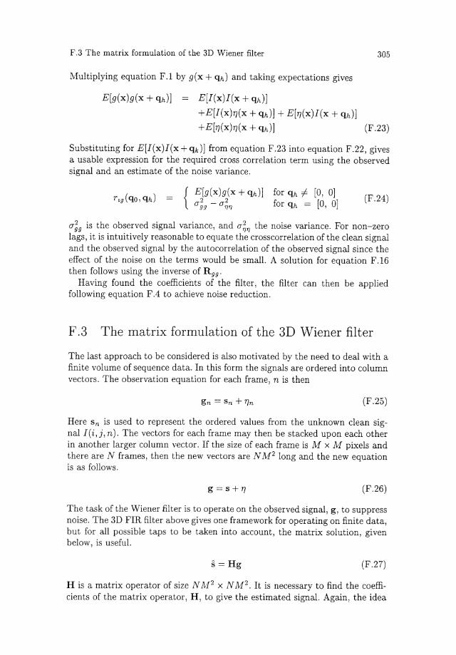
Multiplying equation F.l by g(x + qh) and taking expectations gives

E[g(x)g(x + qh)J E[I(x)I(x + qh)J

+E[I(x)77(x + qh)J + E[77(x)I(x + qh)J +E[r)(x)77(x + qh)J (F.23)

Substituting for E[I(x)I(x + qk)J from equation F.23 into equation F.22, gives a usable expression for the required cross correlation term using the observed signal and an estimate of the noise variance.

for qh f:. [0, OJ for qh = [0, OJ

(F.24)

CJ~g is the observed signal variance, and CJ~'7 the noise variance. For non-zero lags, it is intuitively reasonable to equate the crosscorrelation of the clean signal and the observed signal by the autocorrelation of the observed signal since the effect of the noise on the terms would be small. A solution for equation F.l6 then follows using the inverse of Rgg·

Having found the coefficients of the filter, the filter can then be applied following equation F.4 to achieve noise reduction.

F .3 The matrix formulation of the 3D Wiener filter

The last approach to be considered is also motivated by the need to deal with a finite volume of sequence data. In this form the signals are ordered into column vectors. The observation equation for each frame, n is then

(F.25)

Here sn is used to represent the ordered values from the unknown clean sig­nal I ( i, j, n). The vectors for each frame may then be stacked upon each other in another larger column vector. If the size of each frame is M x M pixels and there are N frames, then the new vectors are N M 2 long and the new equation is as follows.

g=s+7) (F.26)

The task of the Wiener filter is to operate on the observed signal, g, to suppress noise. The 3D FIR filter above gives one framework for operating on finite data, but for all possible taps to be taken into account, the matrix solution, given below, is useful.

s=Hg (F.27)

H is a matrix operator of size N M 2 x N M 2 . It is necessary to find the coeffi­cients of the matrix operator, H, to give the estimated signal. Again, the idea

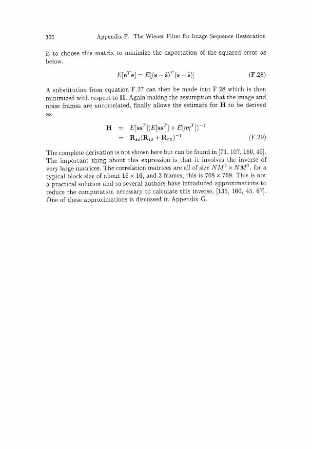
306 Appendix F. The Wiener Filter for Image Sequence Restoration

is to choose this matrix to minimize the expectation of the squared error as

below.

E[eT e] = E[(s- s)T(s- s)] (F.28)

A substitution from equation F.27 can then be made into F.28 which is then

minimized with respect to H. Again making the assumption that the image and

noise frames are uncorrelated, finally allows the estimate for H to be derived

as

H E[ssT](E[ssT] + E[r)1-?])- 1

Rss(Rss + Rry1))-l (F.29)

The complete derivation is not shown here but can be found in [71, 107, 160, 45].

The important thing about this expression is that it involves the inverse of

very large matrices. The correlation matrices are all of size N M 2 x N lvf 2 , for a

typical block size of about 16 x 16, and 3 frames, this is 768 x 768. This is not

a practical solution and so several authors have introduced approximations to

reduce the computation necessary to calculate this inverse, [135, 160, 45, 67].

One of these approximations is discussed in Appendix G.

Appendix G Reducing the Complexity of Wiener Filtering

Although the frequency domain Wiener filter is computationally simple, requir­ing only 3 separable DFT implementations, the matrix formulation of the filter is computationally quite heavy. This formulation is potentially more accurate than the frequency domain implementation since the form takes into account the finite temporal size of the data volume involved. Ozkan et al [135, 42] have developed an efficient solution for this filter form which takes advantage of some approximations about the circulant nature of the correlation matrix of the signals. It is possible to derive their result by an alternative route which is described here after a brief overview of their result.

G.l Efficient Wiener filtering via 2D DFT diagonalization

The signal model is as stated in the previous appendix on Wiener filtering.

g=s+ry (G.1)

The column vectors are made up of the data from N frames ordered and stacked. Therefore,

(G.2)

and so on for the other data vectors, where the frames are indexed from 1 to N.

The matrix Wiener solution was given in the previous appendix. Following Galatsanos et al [45], Ozkan et al [135] noted that the correlation matrices

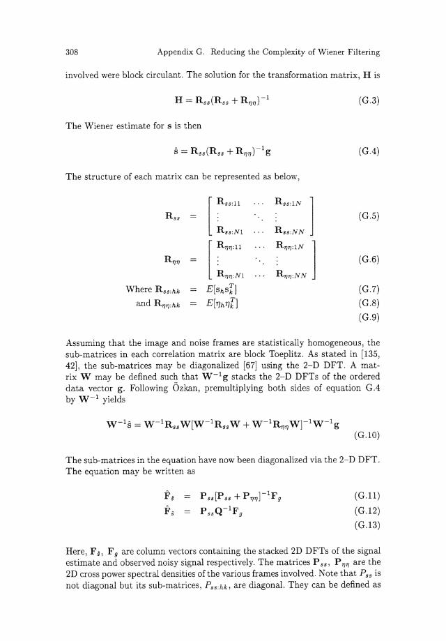
308 Appendix G. Reducing the Complexity of Wiener Filtering

involved were block circulant. The solution for the transformation matrix, H is

The Wiener estimate for s is then

The structure of each matrix can be represented as below,

Where Rss:hk

and R'T/1/:hk

[

~ss:ll

Rss:Nl

[

~1}1):11

R'T}1):Nl

E[shsf]

E[TJhTJfJ

Rss:lN l Rss:NN

l

(G.3)

(G.4)

(G.5)

(G.6)

(G.7)

(G.8)

(G.9)

Assuming that the image and noise frames are statistically homogeneous, the sub-matrices in each correlation matrix are block Toeplitz. As stated in [135, 42], the sub-matrices may be diagonalized [67] using the 2-D DFT. A mat­rix W may be defined such that w- 1g stacks the 2-D DFTs of the ordered data vector g. Following Ozkan, premultiplying both sides of equation G.4 by w-l yields

(G.lO)

The sub-matrices in the equation have now been diagonalized via the 2-D DFT. The equation may be written as

Pss[Pss + P1J1Jt 1F 9

PssQ-lFg

(G.ll)

(G.12)

(G.l3)

Here, F s, F 9 are column vectors containing the stacked 2D DFTs of the signal estimate and observed noisy signal respectively. The matrices P ss, P '7'1/ are the 2D cross power spectral densities of the various frames involved. Note that Pss is not diagonal but its sub-matrices, Pss:hk, are diagonal. They can be defined as

G.l Efficient Wiener filtering via 2D DFT diagonalization 309

below.

[ P.,n Pss:lN

l Pss (G.l4)

P ss:Nl Pss:NN [ r .. ", 0

l where P ss:hk (G.l5)

Pss:hk,Jvi2

[ Qn QrN

l Q (G.l6)

QNl QNN

[ ~"' 0

l where Qhk (G.l7)

Qhk,M 2

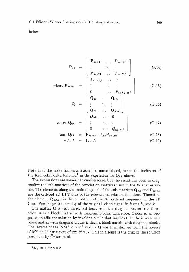
and Qhk P ss:hk + bhkp ~1):hk (G.l8) \;/ h, k l. .. N (G.l9)

Note that the noise frames are assumed uncorrelated, hence the inclusion of the Kronecker delta function 1 in the expression for Qhk above.

The expressions are somewhat cumbersome, but the result has been to diag­onalize the sub-matrices of the correlation matrices used in the Wiener estim­ate. The elements along the main diagonal of the sub-matrices Qhk and P ss:hk

are the ordered 2D DFT bins of the relevant correlation functions. Therefore, the element Pss:hk,l is the amplitude of the lth ordered frequency in the 2D Cross Power spectral density of the original, clean signal in frame h, and k.

The matrix Q is very large, but because of the diagonalization transform­ation, it is a block matrix with diagonal blocks. Therefore, Ozkan et al pro­posed an efficient solution by invoking a rule that implies that the inverse of a block matrix with diagonal blocks is itself a block matrix with diagonal blocks. The inverse of the N M 2 x N M 2 matrix Q was then derived from the inverse of M 2 smaller matrices of size N x N. This in a sense is the crux of the solution presented by Ozkan et al.

1 8hk = lforh=k

310 Appendix G. Reducing the Complexity of Wiener Filtering

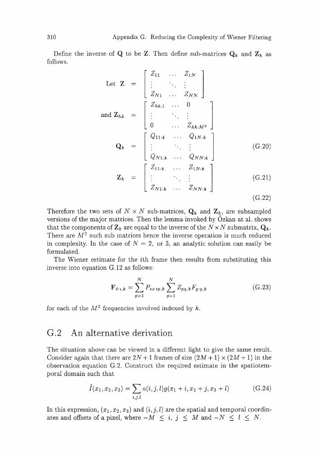
Define the inverse of Q to be Z. Then define sub-matrices Qk and zk as follows.

[ ~n z1N l Let Z

ZNl ZNN [ r .. ,. 0

l and zhk

zhk:M2

[ ~"' QlN:k

l Qk (G.20)

QNl:k QNN:k

zk

[ z,, ~kN,k l (G.21)

ZNl:k ZNN:k

(G.22)

Therefore the two sets of N x N sub-matrices, Qk and Zk, are subsampled versions of the major matrices. Then the lemma invoked by Ozkan at al. shows that the components of Zk are equal to the inverse of the N x N submatrix, Qk.

There are M 2 such sub matrices hence the inverse operation is much reduced in complexity. In the case of N = 2, or 3, an analytic solution can easily be formulated.

The Wiener estimate for the ith frame then results from substituting this inverse into equation G.12 as follows:

N N

FS:z,k = L Pss:ip,k L Zpq,kFg:q,k (G.23) p=l q=l

for each of the Jv! 2 frequencies involved indexed by k.

G.2 An alternative derivation

The situation above can be viewed in a different light to give the same result. Consider again that there are 2N + 1 frames of size (2M+ 1) x (2M+ 1) in the observation equation G.2. Construct the required estimate in the spatiotem­poral domain such that

i(x1, x2, x3) = L a(i, j, l)g(x1 + i, x2 + j, X3 + l) (G.24) i,j,l

In this expression, (x1, x2, x3) and (i, j, l) are the spatial and temporal coordin­ates and offsets of a pixel, where -M :::; i, j :::; M and -N :::; l :::; N.

G.2 An alternative derivation 311

The equation G.24 may be written explicitly as the sum of separate convolu­tions of the observed frames 9i with a set of different coefficients for each frame. If there were 3 frames required for the FIR filter the equation would read:

La(i,j,-1)g(xl +i,xz +j,x3 -1) i,j

+ L a(i, j, O)g(x1 + i, x2 + j, x 3 )

i,j

+ La(i,j,+1)g(xl +i,x2 +j,x3 + 1) i,j

(G.25)

for a non-causal filter using a frame previous to and after the current frame x 3 .

This equation can then be written in the frequency domain, using the 2D DFT, as

A_l (wl, w2)F9 ,x 3 -1 (w1, Wz)

+Ao(wl, w2)F9 ,x 3 (wl, wz)

+A1 (wl, w2)F9 :x 3 +1 (wl, w2) (G.26)

Here, Fs:h(w1 ,w2 ) and F9 ,h(w1,w2) represent the 2D DFT of the hth frame estimate and noisy observed frame respectively. Similarly Aq (w1 , w2 ) represents the 2D DFT of the coefficient mask in the qth offset frame, so that it is applied to frame x 3 +q in this case. The transformed coefficient masks, Ak(w1 ,w2 ) etc., are required.

The 2D DFT of the estimate of the clean signal in frame v can then be represented by

N

Fs,v(wl, wz) = L Aq(wl, wz)Fg,v+q (wl, w2) q=-N

(G.27)

Returning to the spatiotemporal domain, the MMSE (Minimum Mean Squared Error) estimate for the coefficients a( i, j, l) is found by solving the following set of equations (from equation F.15).

t,j,l

E[I(x1,xz,x3)g(x1 + k1,x2 + k2,x3 + k3)] (G.28)

£ { -N < k3 < N or - }vf ;:: k1 , k2 S ll!I

This equation can then be simplified to make clear the correlation measure­ments that are required between frames.

La(i,j,l)r99 x 3 +l,x 3+k 3 (i- k1,j- kz) i,j,l

for {

(G.29)

-N S k3 S N -M S k1, kz S ll!I

312 Appendix G. Reducing the Complexity of Wiener Filtering

Two assumptions are made, spatial homogeneity and that the noise and image frames are not correlated with each other. The solution may be simplified by taking the 2D DFT of the expression to yield

N

L Aq(wl,w2)P99 :x 3 +q,x 3 +k3 (wl,w2) (G.30) q=-N

for - N ~ k3 ~ N

(G.31)

Here, P99 :x3 +q,x 3 +k3 (w1, w2) represents the Cross Power Spectral Density of the noisy frames X3 + q and X3 + k3, and Psg:x 3 ,x3 +k3 (wl,w2) is the required cross power spectral density of the noisy and original frames. Here s is used instead of i as the index to avoid confusion with the use of i as the horizontal offset used in the filter expression.

Equation G .30 represents a set of N equations for the N coefficients Aq ( w1 , w2), at each spatial frequency (w1, w2). The set of equations may be written as, (us­ing a shortened form for the Power Spectral Densities concerned)

[ ~gg:-N,-N(Wl, W2)

P99 ,N,-N(wl, w2)

[ ~sg-N(wl,w2) l Psg:N(wl,w2)

Pgg:x 3 +h,x3 +k ( W1, W2)

Pss:x 3 +h,x 3 +k (wl, W2)

+b'x 3 +h,x 3 +kp7J7J (wl, w2)

Ps9 :x3 ,x3+h (wl, w2)

Pss:x3 ,x3+h

(G.32)

Pss:hk(w1 , w2 ) is the Cross Power Spectrum of the frames in the clean original signal I( i, j, n), similarly for Pry~ (w1 , w2 )). The solution to this matrix equation at each spatial frequency would then yield the 2D DFT of the coefficients in each frame. This result can then be substituted into the frequency domain expression for the filter, equation G.27, to yield the 2D DFT of the estimate for the required frame.

The equation G .32 may be expressed in a more compact form:

Qa=p (G.33)

From this equation the estimate of the clean signal at spatial frequency ( w1 , w2) in the vth frame may be written as

(G.34)

G.3 A final refinement 313

where F 9 is as defined by the terms required in G.27. Letting Z(w1 ,w2) represent the required inverse matrix in equation G.32,

Q- 1 , the following definition is helpful.

[ ~-N,-N(wl, w2)

ZN,-N(wl, w2)

~-N,N(wl, w2) l ZN,N(wl,w2)

(G.35)

Note that the inverses defined in equation G.35 and G.21 are identical matrices because the Qk matrix introduced previously in equation G.20 is the same as the left hand matrix introduced in equation G.32. There is an offset in the indices, but this is due to the definition of the filter.

Given this matrix inverse then, it is possible using G.34 to write the 2D DFT of the estimate in the vth frame as

N N

Fs:v(wl,w2) = L Pss:v,v+p(wl,w2) L Zpq(wl,w2)F9,q(wl,w2) p=-N q=-N (G.36)

Here the 2D DFT of the required estimate of the original clean signal is denoted by F8,v(w1 ,w2 ). Note that again sis used as a synonym fori. This solution is identical to the one given previously in G.23 except for the range of the indices. This depends on the definition of the the filtering operation but does not affect the outcome.

This alternative approach highlights the basic difference between this efficient Wiener solution and the matrix solution discussed previously in Appendix F. It strikes a balance between the fully 3D Frequency approach, which depends on the validity of the DFT of a small number of samples in the temporal direc­tion, and the fully spatiotemporal approach which is computationally intensive. Ozkan et al presented this efficient method with respect to global interframe motion, they went on to incorporate the motion itself into the filter solution.

G. 3 A final refinement

Ozkan et a! recognized that the inverse operation that was required for this new solution could also be computed efficiently. This was allowed if the approxim­ation was made that the power spectra for the noise frames was identical for each frame and that

(G.37)

Which means that the cross power spectral densities of frames p and q can be cakulated by the magnitude of the product of the 2D DFT's of the frames. They show that under these conditions, the inverse of the matrix Qk> defined in equation G.20, can be solved analytically. The final result for the 2D DFT of the required estimate of frame vis stated below. A complete derivation can be found

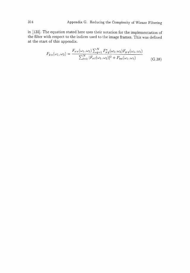
314 Appendix G. Reducing the Complexity of Wiener Filtering

in [135]. The equation stated here uses their notation for the implementation of the filter with respect to the indices used to the image frames. This was defined at the start of this appendix.

Fs:v(wr,w2) 'E~1 F;q(w1,w2)F9 ,q(w1,w2) F.s:u(WI, w2) = N .,

Ll=l1Fs:l(wr,w2)1- + P1J1J(w1,w2) (G.38)

References

[1] I. Abdelqader and S. Rajala. Energy minimisation approach to motion estimation. Signal Processing, 28:291-309, 1992.

[2] Bilge Alp, Petri Haavisto, Tiina Jarske, Kai Oistiimo, and Yrjo Neuvo. Median-based algorithms for image sequence processing. In SPIE Visual Communications and Image Processing, pages 122-133, 1990.

[3] Georgios Angelopoulos and Ioannis Pitas. Least-squares multichannel filters in color image restoration. In Proceedings European Conference on Circuit Theory and Design (ECCTD8g), September 1989.

[4] Georgios Angelopoulos and Ioannis Pitas. Multichannel Wiener filters in color image restoration based on ar color image modelling. In Pro­ceedings IEEE International Conference on Acoustics Speech and Signal Processing (ICASSP ), April 1991.

[5] A. Antoniadis and G. Oppenheim. Wavelets and Statistics. Springer­Verlag, 1995.

[6] G.R. Arce. Multistage order statistic filters for image sequence pro­cessing. IEEE Transactions on Signal Processing, 39:1146-1161, May 1991.

[7] G.R. Arce and R.E. Foster. Multilevel median filters, properties and ef­ficacy. In International Conference on Acoustics Speech and Signal Pro­cessing, pages 824-826, 1988.

316 References

(8] G.R. Arce and E. Malaret. Motion preserving ranked-order filters for im­age sequence processing. In IEEE Int. Conference Circuits and Systems, pages 983-986, 1989.

(9] S. Armstrong, A. Kokaram, and P. J. W. Rayner. Non-linear interpol­ation of missing data using min-max functions. In IEEE International Conference on Nonlinear Signal and Image Processing, July 1997.

(10] J. Astola, P. Haavisto, andY. Nuevo. Vector median filters. Proceedings of the IEEE, 78:678-689, April 1990.

(11] M. Adams B. Levy and A. Willsky. Solution and linear estimation of 2D nearest neighbour models. Proceedings of the IEEE, 78:627-641, April 1990.

(12] M. Barni. A fast algorithm for 1-norm vector median filtering. IEEE Transactions on Image Processing, 6(10):1452-1455, October 1997.

(13] C. Bergeron and E. Dubois. Gradient-based algorithms for block ori­ented map estimation of motion and application to motion-compensated temporal interpolation. IEEE Transactions on Circuits and Systems for Video Technology, 1:72-85, March 1991.

(14] J. M. Bernardo and A. F. M. Smith. Bayesian Theory. Wiley, 1995.

(15] J. Besag. On the statistical analysis of dirty pictures. Journal of the Royal Statistical Society B, 48:259-302, 1986.

(16] Bhavesh Bhatt, David Birks, and David Hermreck. Digital television: making it work. IEEE Spectrum, pages 19-28, October 1997.

(17] J. Biemond, L. Looijenga, D. E. Boekee, and R.H.J.M. Plompen. A pel-recursive Wiener based displacement estimation algorithm. Signal Processing, 13:399-412, 1987.

[18] M. Bierling. Displacement estimation by heirarchical block matching. In SPIE VCIP, pages 942-951, 1988.

(19] G. Wooi Boon, M. N. Chong, S. Kalra, and D. Krishnan. Bidirectional 3D autoregressive model approach to motion picture restoration. In IEEE International Conference on Acoustics and Signal Processing, pages 2275-2278, April 1996.

(20] L. Boroczky, J. N. Driessen, and J. Biemond. Adaptive algorithms for pel-recursive displacement estimation. In Proceedings SPIE VCIP, pages 1210-1221, 1990.

(21] L. Boroczky, K. Fazekas, and T. Szabados. Convergence analysis of a pel­recursive Wiener based motion estimation algorithm. In Time Varying Image Processing and Moving Object Recognition 2, pages 38-45. Elsevier, 1990.

References 317

[22) G. E. P. Box and G. C. Tiao. Bayesian Inference in Statistical Analysis. Addison-Wesley, 1973.

[23) J. Boyce. Noise reduction of image sequences using adaptive motion compensated frame averaging. In IEEE ICASSP, volume 3, pages 461-464, 1992.

[24) D. B. Bradshaw, N. G. Kingsbury, and A. C. Kokaram. A gradient based fast search algorithm for warping motion compensation schemes. In IEEE International Conference on Image Processing, pages 187-190. IEEE, October 1997.

[25) P. Burt and E. Adelson. The Laplacian pyramid as a compact image code. IEEE transactions on Communications, 31:532-540, April 1983.

[26) C. Cafforio and F. Rocca. Methods for measuring small displacements of television images. IEEE transactions on Information Theory, 22:573-579, 1976.

[27) John Canny. A computational approach to edge detection. IEEE Trans­actions on Pattern Analysis and Machine Intelligence, 8(6):679-698, 1986.

[28) M. N. Chong, P. Liu, W. B. Goh, and D. Krishnan. A new spatia­temporal MRF model for the detection of missing data in image se­quences. In IEEE International Conference on Acoustics and Signal Pro­cessing, volume 4, pages 2977-2980, April 1997.

[29) E. Coyle, J. Lin, and M. Gabboui. Optimal stack filtering and the es­timation and structural approaches to image processing. IEEE Transac­tions on Acoustics, Speech and Signal Processing, 37:2037-2065, Decem­ber 1989.

[30) S. C. Dabner. Real time motion vector measurement hardware. In 3rd International Workshop on HDTV, Aug. 1989.

(31) T. Dennis. Nonlinear temporal filter for television picture noise reduc­tion. lEE Proceedings, 127:52-56, April 1980.

[32) H. Derin and P. Kelly. Discrete-index Markov-type random processes. Proceedings of the IEEE, 77:1485-1509, October 1989.

[33] J. Driessen, R. Belfor, and J. Biemon<i. Backward predictive motion compensated image sequence coding. In Signal Processing V: Theories and Applications, pages 757-760, 1990.

(34) J. Driessen, J. Biemond, and D. Boekee. A pel-recursive segmentation and estimation algorithm for motion compensated image sequence coding. In IEEE ICASSP, pages 1901-1904, 1989.

318 References

[35] J. Driessen, L. Boroczky, and J. Biemond. Pel-recursive motion field es­timation from image sequences. Visual Communication and Image Rep­resentation, 2:259-280, 1991.

[36] E. Dubois and S. Sabri. Noise reduction in image sequences using motion compensated temporal filtering. IEEE Transactions on Communications, 32:826-831, July 1984.

[37] S. Efstratiadis and A. Katsagellos. A model based, pel-recursive motion estimation algorithm. In Proceedings IEEE ICASSP, pages 1973-1976, 1990.

[38] S. Efstratiadis and A. Katsaggelos. A multiple-frame pel-recursive Wiener-based displacement estimation algorithm. In SPIE VCIP IV, pages 51-60, 1989.

[39] David P. Elias and Nick G. Kingsbury. The recovery of a near optimal layer representation for an entire image sequence. In Proceedings IEEE International Conference on Image Processing, 1997.

[40] David P. Elias and K. K. Pang. Obtaining a coherent motion field for motion based segmentation. In Picture Coding Symposium, pages 541-546, 1996.

[41] W. Enkelmann. Investigations of multigrid algorithms for the estimation of optical flow fields in image sequences. Computer Vision Graphics and Image Processing, 43:150-177,1988.

[42] A. Erdem, M. Sezan, and M. Ozkan. Motion-compensated multiframe Wiener restoration of blurred and noisy image sequences. In IEEE ICASSP, volume 3, pages 293-296, March 1992.

[43] J. Patrick Fitch, Edward J. Coyle, and Neal C. Gallagher. Median fil­tering by threshold decomposition. IEEE Trans. Acoustics and Signal Processing, 32:1183-1188, December 1984.

[44] S. Fogel. The estimation of velocity vector fields from time-varying im­age sequences. Computer Vision Graphics and Image Processing: Image Understanding, 53:253-287, May 1991.

[45] N. Galatsanos and R. Chin. Digital restoration of multichannel images. IEEE Transactions on ASSP, 37:415-421, March 1989.

[46] Neal C. Gallagher and Gary L. Wise. A theoretical analysis of the prop­erties of median filters. IEEE Trans. Acoustics and Signal Processing, 29:1136-1141, December 1981.

[47] S. Geman and D. Geman. Stochastic relaxation, gibbs distributions and the Bayesian restoration of images. IEEE Transactions on Pattern Ana­lysis and Machine Intelligence, 6:721-741, 1984.

References 319

[48] S. Geman and D. McClure. A nonlinear filter for film restoration and other problems in image processing. CVGIP, Graphical Models and Im­age Processing, 54:281-289, July 1992.

[49] M. Ghanbari. The cross-search algorithm for motion estimation. IEEE Transactions on Communications, 38:950-953, July 1990.

[50] B. Girod. Motion-compensating prediction with fractional-pel accuracy. IEEE Transactions on Communications, Accepted March 1991.

[51] S. Godsill. Restoration of Degraded Audio Signals. PhD thesis, Cam­bridge University Engineering Dept., 1994.

[52] S. Godsill and A. Kokaram. Joint interpolation, motion and parameter estimation for degraded image sequences with missing data. In Signal Processing VIII, volume I, pages 1-4, September 1996.

[53] S. Godsill and A. Kokaram. Restoration of image sequences using a causal spatio-temporal model. In The Art and Science of Bayesian Image Analysis, pages 189-194, July 1997.

[54] S. Godsill and P. Rayner. A Bayesian approach to the detection and correction of error bursts in audio signals. In IEEE ICASSP, volume 2, pages 261-264, 1992.

[55] S. J. Godsill. Bayesian enhancement of speech and audio signals which can be modelled as ARMA processes. International Statistical Review, 65(1):1-21, 1997.

[56] P.J. Green. Reversible Jump MCMC computation and Bayesian model determination, September 1994.

[57] Tom R. Halfhill. CDs for the gigabyte era. Byte magazine, pages 139-144, October 1996.

[58] Barry G. Haskell, Atul Puri, and Arun N. Netravali. Digital Video: An Introduction to MPEG-2. Chapman Hall, 1997.

[59] David J. Heeger and James R. Bergen. Pyramid-based texture ana­lysis/synthesis. In IEEE International Conference on Image Processing, pages 648-651, October 1995.

[60] F. Heitz and Bouthemy. Motion estimation and segmentation using a global bayesian approach. In Proceedings ICASSP, 1990.

[61] F. Heitz and Bouthemy. Multimodal motion estimation and segmentation using markov random fields. In Proceedings International Conference on Pattern Recognition, pages 378-383, 1990.

[62] H. Higgins. The interpretation of a moving retinal image. Proceedings of the Royal Society, London, B 208:385-397, 1980.

320 References

[63] H. Higgins. The visual ambiguity of a moving plane. Proceedings of the Royal Society, London, B 223:165-175, 1984.

[64] Anil N. Hirani and Takashi Totsuka. Combining frequency and spatial domain information for fast interactive image noise removal. In Proceed­ings SIGGRAPH, pages 269-276, 1996.

[65] B. Horn and B. Schunck. Determining optical flow. Artificial Intelligence, 17:185-203, 1981.

[66] T. Huang. Image Sequence Analysis. Springer-Verlag, 1981.

[67] B. Hunt. The application of constrained least squares estimation to im­age resoration by digital computer. IEEE Transactions on Computers, 22:805-812, September 1973.

[68] Keith Jack. Video Demystified. Hightext, 1993.

[69] A. Jain. Partial differential equations and finite-difference methods in im­age representing, Part 1: Image representation. Journal of Optimization Theory and Application, pages 65-91, September 1977.

[70] A. Jain and J. Jain. Partial differential equations and finite difference in image processing Part 2: Image restoration. IEEE Transactions on Automatic Control, pages 817-834, October 1978.

[71] A.K. Jain. Fundamentals of Digital Image Processing. Prentice Hall, 1989.

[72] Ronald J. Jurgen. Digital video. IEEE Spectrum, pages 24-30, March 1992.

[73] D. Kalivas and A. Sawchuk. Motion compensated enhancement of noisy image sequences. In IEEE ICASSP, volume 1, pages 2121-2124, 1990.

(74] R. H. Kallenberger and G. D. Cvjetnicanin. Film into Video. Focal Press, 1994.

[75] S. Kalra, M. N. Chong, and D. Krishnan. A new autoregressive (AR) model based algorithm for motion picture restoration. In IEEE Interna­tional Conference on Acoustics and Signal Processing, pages 2557-2560, April 1997.

[76] S. Karunasekera and N. Kingsbury. A distortion measure for blocking artifacts in images based on human visual sensitivity. IEEE Transactions on Image Processing, 4(6):713-724, June 1995.

(77] A. Katsagellos, J. Driessen, S. Efstratiadis, and R. Lagendijk. Spatia­temporal motion compensated noise filtering of image sequences. In SP IE VCIP, pages 61-70, 1989.

References 321

[78] J. Kearney, W.B. Thompson, and D. L. Boley. Optical flow estimation: An error analysis of gradient based methods with local optimisation. IEEE Transactions on Pattern Analysis and Machine Intelligence, pages 229-243, March 1987.

[79] R. Kleihorst. Noise Filtering of Image Sequences. PhD thesis, Inform­ation Theory Group, Delft University of Technology, The Netherlands, 1994.

[80] R. Kleihorst, G. de Haan, R. Lagendijk, and J. Biemond. Motion com­pensated noise filtering of image sequences. In Signal Processing VI, pages 1385-1388. Elsevier Science, 1992.

[81] A. Kokaram. 3D Wiener filtering for noise suppression in motion picture sequences using overlapped processing. In Signal Processing V, Theories and Applications, pages 1780-1783, September 1994.

[82] A. Kokaram and W. J. Fitzgerald. Image processing applied to ancient manuscripts. In 20th International Congress of Papyrologists., August 1992.

[83] A. Kokaram and S. Godsill. A system for reconstruction of missing data in image sequences using sampled 3D AR models and MRF motion pri­ors. In European Conference on Computer Vision 1gg6, pages 613-624. Springer-Verlag, April 1996.

[84] A. Kokaram and S. Godsill. Joint detection, interpolation, motion and parameter estimation for image sequences with missing data. In IEEE International Conference on Image Processing, pages 191-194. IEEE, Oc­tober 1997.

[85] A. Kokaram and S. Godsill. Joint detection, interpolation, motion and parameter estimation for image sequences with missing data. In Im­age Analysis and Processing, volume 2, pages 719-725. Springer-Verlag, September 1997.

[86] A. Kokaram, R. Morris, W. Fitzgerald, and P. Rayner. Detection of missing data in image sequences. IEEE Image Processing, pages 1496-1508, November 1995.

[87] A. Kokaram, R. Morris, W. Fitzgerald, and P. Rayner. Interpolation of missing data in image sequences. IEEE Image Processing, pages 1509-1519, November 1995.

[88] A. Kokaram, N. Persad, J. Lasenby, W. Fitzerald, A. McKinnon, and M. Welland. Restoration of images from the scanning tunnelling micro­scope. Applied Optics, 34(23):5121-5131, August 1995.

[89] A. Kokaram and P. Rayner. An algorithm for line registration of TV images based on a 2-D AR model. In Signal Processing VI, Theories and Applications, pages 1283-1286, August 1992.

322 References

[90] A. Kokaram and P. Rayner. Removal of impulsive noise in image se­quences. In Singapore International Conference on Image Processing., pages 629-633, September 1992.

[91] A. Kokaram and P. Rayner. A system for the removal of impulsive noise in image sequences. In SPIE Visual Communications and Image Pro­cessing, pages 322-331, November 1992.

[92] A. Kokaram and P. Rayner. Detection and interpolation of replacement noise in motion picture sequences using 3D autoregressive modelling. In IEEE International Symposium on Circuits and Systems, pages 21-24, June 1994.

[93] A. Kokaram and P. Rayner. Removal of replacement noise in motion picture sequences using 3D autoregressive modelling. In Signal Processing V, Theories and Applications, pages 1760-1763, September 1994.

[94] A. Kokaram, P. M. B. Roosmalen, P. J. W. Rayner, and J. Biemond. Line registration of jittered video. In IEEE International Conference on Acoustics Speech and Signal Processing, pages 2553-2556, April 1997.

[95] A. Kokaram, A. Stark, and W. J. Fitzgerald. Enhancement and restor­ation of ancient manuscripts. In SPIE Conference on Applications of Digital Image Processing XV., pages 322-331, July 1992.

[96] A. C. Kokaram. Motion Picture Restoration. PhD thesis, Cambridge University, England, May 1993.

[97] A. C. Kokaram. Reconstruction of severely degraded image sequence. In Image Analysis and Processing, volume 2, pages 773-780. Springer­Verlag, September 1997.

[98] J. Konrad and E. Dubois. Bayesian estimation of motion vector fields. IEEE Transactions on Pattern Analysis and Machine Intelligence, 14(9), September 1992.

[99] E. E. Kuruoglu. Signal estimation in non-gaussian noise using polynomial filters. Master's thesis, Cambridge University, England, 1995.

[100] E. E. Kuruoglu, P. J. W. Rayner, and W. J. Fitzgerald. Impulsive noise elimination using polynomial iteratively reweighted least squares. In IEEE Workshop on Digital Signal Processing, September 1996.

[101] E. E. Kuruoglu, P. J. W. Rayner, and W. J. Fitzgerald. Least lp-norm estimation of autoregressive model coefficients of symmetric a-stable pro­cesses. IEEE Signal Processing Letters, pages 201-204, july 1997.

[102] R. L. Lagendijk and J. Biemond. Iterative Identification and Restoration of Images. Kluwer Academic Publishers, 1991.

References 323

[103] S. Z. Li. Discontinuity-adaptive MRF prior and robust statistics: A com­paritive study. Image and Vision Computing, pages 227-223, April 1995.

[104] S. Z. Li. Markov Random Field Modeling in Computer Vision. Springer­Verlag, 1995.

[105] S. z. Li. On disontinuity-adaptive smoothness priors in computer vision. IEEE Transactions on Pattern Analysis and Machine Intelligence, pages 576-586, june 1995.

[106] J. S. Lim. Image restoration by short space spectral subtraction. IEEE ASSP, 28:191-197, April 1980.

[107] Jae S. Lim. Two-Dimensional Signal and Image Processing. Prentice­Hall, 1990.

[108] J. Lin, T. Sellke, and E. Coyle. Adaptive stack filtering under the mean absolute error criterion. IEEE Transactions on Acoustics, Speech and Signal Processing, 38:938-954, June 1991.

[109] J. Liu, W. H. Wong, and A. Kong. Covariance structure of the Gibbs sampler with applications to the comparison of estimators and augment­ation schemes. Biometrika, 81:27-40, 1994.

[110] J. F. A. Magarey, A. C. Kokaram, and N. G. Kingsbury. Optimal schemes for motion estimation on colour image sequences. In IEEE International Conference on Image Processing, pages 187-190. IEEE, October 1997.

[111] J. F. A. Magarey, A. C. Kokaram, and N. G. Kingsbury. Robust mo­tion estimation using chrominance information in colour image sequences. In Image Analysis and Processing, volume 2, pages 486-493. Springer­Verlag, September 1997.

[112] Julian F. A. Magarey. Motion estimation using complex wavelets. PhD thesis, Cambridge University, England, 1997.

[113] S.G. Mallat. Multifrequency channel decompositions of images and wave­let models. IEEE Transactions on Acoustics, Speech and Signal Pro­cessing, pages 2091-2110. December 1989.

[114] D. Marr. Vision. W. H. Freeman and Company, 1982.

[115] D. Martinez and J. Lim. Implicit motion compensated noise reduction of motion video scenes. In IEEE ICASSP, pages 375-378, 1985.

[116] D. Martinez and J. Lim. Spatial interpolation of interlaced television pictures. In IEEE ICASSP, volume M9.21, pages 1886-1889, 1989.

[117] D. M. Martinez. Model-based motion estimation and its application to restoration and interpolation of motion pictures. PhD thesis, Massachu­setts Institute of Technology, 1986.

324 References

[118] R. D. Morris. Image Sequence Restoration using Gibbs Distributions. PhD thesis, Cambridge University, England, 1995.

[119] R. D. Morris and W. J. Fitzgerald. Detection and correction of speckle degradation in image sequences using a 3D markov random field. In Proceedings International Conference on Image Processing : Theory and Applications (!PTA '93). Elsevier, June 1993.

[120] R. D. Morris and W. J. Fitzgerald. Replacement noise in image sequences, detection and interpolation by motion field segmentation. In IEEE International Conference on Acoustics and Signal Processing (ICASSP), 1994.

[121] R. D. Morris and W. J. Fitzgerald. Stochastic and deterministic methods in motion picture restoration. In Proceedings International Workshop on Image Processing, June 1994.

[122] R. D. Morris and W. J. Fitzgerald. Discontinuous motion and occlu­sion estimation: Theory and application. In Proceedings International Conference for Young Computer Scientists (ICYCS), September 1996.

[123] M. J. Nadenau and S. K. Mitra. Blotch and scratch detection in image sequences based on rank ordered differences. In 5th International Work­shop on Time- Varying Image Processing and Moving Object Recognition, September 1996.

[124] H. Nagel. Constraints for the estimation of displacement vector fields from image sequences. In International Joint Conference on Artificial Intelligence., pages 945-951, 1983.

[125] H. Nagel. Displacement vectors derived from second order intensity vari­ations in image sequences. Computer Vision, Graphics and Image Pro­cessing, 21:85-117, 1983.

[126] H. Nagel. Recent advances in image sequence analysis. In Premiere Coloque Image Traitment, Synthese, Technologie et Applications., pages 545-558, May 1984.

[127] H. Nagel. Spatia-temporal modeling based on image sequences. In In­ternational Symposium on Image Processing and its Applications., pages 222-252, 1984.

[128] H. Nagel. Towards the estimation of displacement vector fields by 'ori­ented smoothness' constraints. In International Joint Conference on Pat­tern Recognition, pages 6-8, 1984.

[129] H. Nagel. Image sequences -ten (octal) years - from phenomenology towards a theoretical foundation. In IEEE ICASSP, pages 1174-1185, 1986.

References 325

(130] H. Nagel. On a constraint equation for the estimation of displacement rates in image sequences. IEEE Transactions on Pattern Analysis and Machine Intelligence, 11:13-30, January 1989.

(131] H. Nagel and W. Enkelmann. An investigation of smoothness constraints for the estimation of displacement vector field from image sequences. IEEE Transactions on Pattern Analysis and Machine Intelligence, 8:565-592, September 1986.

(132] A. Netravali and J. Robbins. Motion-compensated television coding: Part 1. The Bell System Technical Journal, 58:631-670, March 1978.

(133] A. Netravali and J. Robbins. Motion-compensated coding: Some new results. The Bell System Technical Journal, 59:1735-1745, November 1980.

(134] A. Nieminen, P. Heinonen, and Y. Nuevo. A new class of detail­preserving filters for image processing. IEEE Transactions on Pattern Analysis and Machine Intelligence, 9:74-90, January 1987.

(135] M. Ozkan, A. Erdem, M. Sezan, and A. Tekalp. Efficient multiframe Wiener restoration of blurred and noisy image sequences. IEEE Trans­actions on Image Processing, 1:453-476, October 1992.

(136] M. Ozkan, M. Sezan, and A. Erdem. LMMSE restoration of blurred and noisy image sequences. In SPIE VCIP, pages 743-754, 1991.

[137] M. Ozkan, M. Sezan, and A. Tekalp. Motion-adaptive weighted averaging for temporal filtering of noisy image sequences. In SP IE Image Processing Algorithms and Techniques III, pages 201-212, February 1992.

[138] F. Paisan and A. Crise. Restoration of signals degraded by impulsive noise by means of a low distortion, non-linear filter. Signal Processing, 6:67-76, 1984.

(139] I. Pitas and P. Tsakalides. Multivariate ordering in colour image filter­ing. IEEE Transactions on Circuits and Systems for video technology, September:247-259, October 1991.

(140] I. Pitas and A. N. Venetsanopoulos. Nonlinear Digital Filters Principles and Applications. Kluwer Academic Publishers, 1990.

(141] W. K. Pratt. Digital Image Processing. Wiley, 1978.

(142] William H. Press, Saul A. Teukolsky, William T. Vetterling, and Brian P. Flannery. Numerical Recipes in C, The Art of Scientific Computing. Cambridge University Press, 2nd edition, 1992.

[143] Gregory C. Reinsel. Elements of Multivariate Time Series Analysis. Springer-Verlag, 1993.

326 References

[144] J. Riveros and K. Jabbour. Review of motion analysis techniques. fEE Proceedings, 136:397~404, December 1989.

[145] J. Robbins and A. Netravali. Image Sequence Processing and Dynamic Scene Analysis., chapter Recursive Motion Compensation: A Review, pages 76~103. Springer~Verlag, 1983.

[146] Peter M. B. Van Roosmalen, R. L. Lagendijk, and J. Biemond. Correction of intensity flicker in old film sequences. Submitted to: IEEE Transactions on Circuits and Systems for Video Technology, December 1996.

[147] Peter l'vi. B. Van Roosmalen, R. L. Lagendijk, and J. Biemond. Flicker reduction in old film sequences. In Time-varying Image Processing and Moving Object Recognition 4, pages 9~ 17. Elsevier Science, 1997.

[148] Peter l'vi. B. Van Roosmalen, S. J. P. Westen, R. L. Lagendijk, and J. Biemond. Noise-reduction for image sequences using an oriented pyr­amid thresholding technique. In IEEE International Conference on Im­age Processing, volume 1, pages 375~378. IEEE, 1996.

[149] A. Rosenfeld, editor. Univariate and Multivariate random fields for im­ages, pages 245~258. Academic Press, 1981.

[150] A. Rosenfeld and A. Kak. Digital Picture Processing. Academic Press, 1982.

[151] J. J. 0 Ruanaidh and W. J. Fitzgerald. Numerical Bayesian Methods Ap­plied to Signal Processing. Springer~ Verlag, Springer Series in Statistics and Computing, 1996.

[152] Theodore S. Rzeszewski, editor. Digtal Video (Concepts and Applications across Industries). IEEE, 1995.

[153] R. Schalkoff. Digital Image Processing and Computer Vision. Wiley, 1989.

[154] B. Schunck. Image flow: fundamentals and future research. In IEEE ICASSP, pages 560~571, 1985.

[155] B. Schunck. The image flow constraint equation. Computer Vision, Graphics and Image Processing, 35:20~46, 1986.

[156] M. Sezan, M. Ozkan, and S. Fogel. Temporally adaptive filtering of noisy image sequences using a robust motion estimation algorithm. In IEEE ICASSP, volume 3, pages 2429~2431, May 1991.

[157] M. Ibrahim Sezan and R. L. Lagendijk. Motion Analysis and Image sequence Processing. Kluwer Academic, 1993.

[158] Thomas Sikora. Mpeg digital video-coding standards. IEEE Signal pro­cessing magazine, pages 82~ 100, September 1997.

References 327

[159] P. S. Spencer. System identification with application to the restoration of archived Gramophone recordings. PhD thesis, Cambridge University, England, 1990.

[160] C. Srinivas. A stochastic model-based approach for simultaneous restor­ation of multiple misregistered images. In SPIE VCIP, pages 1416-1427, 1990.

[161] R. Srinivasan. Image restoration by spatial filter design. In SPIE VCIP, pages 193-197, 1986.

[162] C. Stiller. Motion-estimation for coding of moving video at 8kbit/sec with gibbs modelled vectorfield smoothing. In SPIE VCIP., volume 1360, pages 468-476, 1990.

[163] R. Storey. Electronic detection and concealment of film dirt. UK Patent Specification No. 2139039, 1984.

[164] R. Storey. Electronic detection and concealment of film dirt. SMPTE Journal, pages 642-647, June 1985.

[165] P. Strobach. Quadtree-structured linear prediction models for image se­quence processing. IEEE Transactions on Pattern Analysis and Machine Intelligence, 11:742-747, July 1989.

[166] T. Strohmer. Computationally attractive reconstruction of bandlimited images from irregular samples. IEEE Image Processing, pages 540-548, April 1997.

[167] Kaijun Tang, Jaakko Astola, and Yrjo Neuvo. Adaptive nonlinear mul­tivariate image filtering for mixed noise removal. In Proceedings Interna­tional Conference of Circuits and Systems, pages 427-430, 1993.

[168] Martin. A. Tanner. Tools for Statistical Inference. Springer-Verlag, 1996.

[169] A. Murat Tekalp. Digital Video Processing. Prentice Hall, 1995.

[170] Jim Teter. Precise film recorders for motion: They came from hollywood. Advanced Imaging Magazine, pages 40-41, January 1992.

[171] C. Therrien. Statistical model-based algorithms for image analysis. IEEE Proceedings, 74:532-551, April 1986.

[172] C. Therrien. Decision Estimation and Classification. Wiley, 1989.

[173] G. Thomas and H. Lau. Generation of high quality slow motion replay using motion compensation. In lEE Conference (IBC 1990), Sept. 1988.

[174] G. A. Thomas. TV Picture motion measurement. UK Patent Specifica­tion No. GB2 188510A, Sept. 1987.

328 References

[175] G. A. Thomas. Distorting the time axis; motion compensated image processing in the studio. In lEE Conference (IBC 1988), pages 256-259, Sept. 1988.

[176] W. B. Thompson, K. M. Mutch, and V. A. Berzins. Dynamic occlusion analysis in optical flow fields. IEEE Transactions on Pattern Analysis and Machine Intelligence, 7:374-383, July 1985.

[177] P. E. Trahanias and A. N. Venetsanopoulos. Vector directional filters. IEEE Transactions on Image Processing, 2:528-534, October 1993.

[178] E. Trundle. TV and Video Technology. Newnes, 1996.

[179] J. Tukey. Exploratory Data Analysis. Addison-Wesley, 1977.

[180] Adrian Turner, Helen MacKintosh, and David Francis OBE. Guide to the Museum of the Moving Image. British Film Institute, 1988.

[181] K. Uomori, A. Morimura, and H. Ishii. Electronic image stabilisation system for video cameras and VCR's. SMPTE Journal, pages 66-75, February 1992.

[182] S. V. Vaseghi. Algorithms for the Restoration of Archived Gramophone Recordings. PhD thesis, Cambridge University, England, 1988.

[183] S. V. Vaseghi and P. J. W. Rayner. Detection and suppression of impuls­ive noise in speech communication systems. Proceedings lEE, 137:38-46, 1990.

[184] R. Veldhuis. Restoration of lost samples in Digital Signals. Prentice Hall, 1980.

[185] Martin Vetterli and Jelena Kovacevic. Wavelets and Subband Coding. Prentice Hall, 1995.

[186] T. Vlachos. Improving the efficiency of MPEG-2 coding by means of film unsteadiness correction. In Proceedings SPIE Conference on Digital Compression Technology and Systems, volume 2952, pages 534-538, Oc­tober 1996.

[187] T. Vlachos. Simple method for the estimation of global motion paramet­ers using sparse translational motion vector fields. To appear in Elec­tronic Letters, 1998.

[188] T. Vlachos and G. A. Thomas. Motion estimation for the correction of twin-lens telecine flicker. In Proceedings IEEE International Conference on Image Processing, volume 1, pages 109-112, September 1996.

[189] D. Walker and K. Rao. Improved pel-recursive motion compensation. IEEE transactions on communications, 32:1128-1134, October 1984.

References 329

[190] John Y. A. Wang and Edward H. Adelson. Representing moving im­ages with layers. IEEE Transactions on Image Processing, 5(3):625-638, September 1994.

[191] G. Winkler. Image Analysis, Random Fields and Dynamic Monte Carlo Methods. Springer-Verlag, 1995.

[192] J. Woods. Two-dimensional discrete Markovian fields. IEEE Transac­tions on Information Theory, pages 232-240, March 1972.

[193] J. Woods. Markov image modelling. IEEE Transactions on Automatic Control, pages 846-850, October 1978.

[194] E. M. Yeh, A. C. Kokaram, and N. G. Kingsbury. Perceptual distor­tion measure for edge-like artifacts in image sequences. In SPIE Human Vision and Electronic Imaging III, volume 3299. SPIE, January 1998.

[195] Olli Yli-Harja. Median Filters: Extensions, Analysis and Design. PhD thesis, Lappeenranta University of Technology, 1989.

[196] R. Young and N. Kingsbury. Video compression using lapped transforms for motion estimation/compensation and coding. In SPIE VCIP, pages 276-288, 1992.

[197] A. Zaccarin and B. Liu. Fast algorithms for block motion estimation. In IEEE ICASSP, volume 3, pages 449-452, 1992.

Index

2D Autoregressive Model, 100-101, 235

Boundary constraints, 235 Non-homogeneous, 101,107,235 Parameter estimation, 107 Sampled interpolation, 238

2DAR, see 2D Autoregressive Model 3D Autoregressive Model, 28-32, 48,

152, 279 Conditional distribution, 154 Correlation, 278 Generating sequences, 51 Motion estimation, 50

Adaptive, 67 Multiresolution, 70

Multichannel, 263 Parameter Estimation

Least Squares, 279 Parameter estimation

Least Squares, 30, 48, 273 Wiener Based, 30 Wiener based, 49

3D Wiener filter, 241, 301, 307 FIR, 246, 251 IIR, 242-243, 251 Noise margin, 245

Overlapped processing, 244 Real data, 255 SNR, 252

3DAR, see 3D Autoregressive Model

BABOON, 58, 94, 219 Bayes theorem, 38, 138, 153 Bayesian Inference

Maximum a Posteriori, 217 Bayesian inference

Gaussian approximation, 41 Iterated Conditional Modes, 43 Maximum a Posteriori, 43 Maximum Likelihood, 41 Metropolis algorithm, 42 Posterior distribution, 211

Block matching, see Motion Estim­ation, 25

Blotches, see Missing Data, 120

CARTOON, 256 Clique, 39, 139, 155 Colour

Decorrelating transform, 265 Detecting missing data, 261-262 Model based reconstruction, 263

264

332

Vector median, 262-263 Colour space, 264 Composition sampling, 157

Data windowing, 244, 24 7 Deblurring, 3 DFT, 243

Film and video artefacts, 6-9 Blotches, 6 Dirt and Sparkle, 6 Flicker, 8 Kinescope Moire, 8 Noise, 7 Unsteadiness, 7

Film Scratches, 227-240 2D Autoregressive model, 235 Degradation model, 229 Detection, 230

Bayesian refinement, 233 Hough Transform, 231 Reconstruction, 235

Tiling, 235 Windowing, 235

Sampled interpolation, 238 Flicker, 8 FRANK, 192

Gibbs energy priors, 39, 138, 155 Gibbs Sampler, see Markov Chain

Monte Carlo Gradient motion estimation, see Mo­

tion Estimation

Half-cosine data window, 244 Hammersley-Clifford, 39 Heuristics, 119 History of film and video, 4

Colour, 5 DVD, 6 George Eastman, 4 Lumiere, 4 Nickelodeon, 4 Sound, 5 Television, 5 Video Tape, 5

Hough Transform, 231

HTML, 4

Jitter Suppression, 99-118 Algorithm, 108

Index

Displacement estimation, 101 Ill-posed, 112 Increasing stability, 105 Multiresolution, 108 Real data, 113 Trend removal, 112 Two Dimensional AR Model,

100 JOMBADI, 158, 225, 287-294

Relation to other systems, 163-177

JUGGLER, 73

LENNA, 219

Markov Chain Monte Carlo, 37 Gibbs sampler, 37, 157, 211, 233

Adaptations, 157, 213 Griddy, 42, 158, 213

ICM, 43, 172, 217 Metropolis algorithm, 42

Markov Random Field, 39, 138 Markov Random Fields, 39 Maximum a Posteriori, 140 MCMC, see Markov Chain Monte

Carlo Median filter, 92

CUBE, 136 LIN, 136 Vector median, 262

Metropolis algorithm, 42 Mirror constraint, 209 Missing Data

Bayesian inference JOMBADI, 158 Morris, 170 Performance, 181 Posterior distribution, 153 Priors for corruption, 155-156 The Likelihood, 154

Causes of, 6 Detection

Morris, 173

Index

Performance of heuristics, 130-135

Pre-processors, 125 Rank Order Detector, 124 ROD, 124, 175, 221 SDI, 123 SDia, 122 SDip, 123 Spike Detection Index, 122

Dirt and Sparkle, 2 Fast interpolation, 177 Godsill, 175 Impulsive noise, 92 Joint detection and reconstruc­

tion, 153-162 Large areas, 201

Algorithm, 214 Bayesian inference, 211 Gibbs sampler, 213 Motion interpolation, 204-208 Multiresolution, 213 Performance, 218

Model based treatment, 151 Motion estimation, 126 Motion interpolation, 137-142 Rayner, 175 Reconstruction

Median filters, 135, 136, 142 Real data, 142-149 System, 150

Richard Storey, 122 Scratch removal, see Film Scratches SDI, see Spike Detection Index Two step removal, 120-121 Vaseghi, 175

MMF, see Multilevel median filter MOBCAL, 130, 181, 250 Motion Estimation

3D Autoregressive model, 282 Bayesian inference, 36

Gaussian approximation, 41 Gibbs sampler, 37 Iterated Conditional Modes,

43 Markov Random Fields, 39 Maximum a Posteriori, 43

333

Maximum Likelihood, 41 MRF priors for motion edges,

44 Occlusion, 210 Smoothness priors, 42, 155,

208, 209 Block matching, 16, 18 Comparison, 126-130 Correspondence matching, 16 Direct search, 16 Gradient based, 18-25, 282

Til-conditioning, 295 m.-conditioning, 23-24

Multiresolution, 32-34, 70 Occlusion priors, 210 Optical flow, 24, 43 Smoothness constraints, 24 Temporal smoothness, 209 Wiener based, 20-21, 101-105 With missing data, 137-142

Multilevel median filter, 92 Alp, 135 Arce, 135 BI, 135 ML3D, 135 ML3Dex, 137 Vector ML3Dex, 263

Noise, 7 Noise floor, 246 Noise Reduction

Motion compensation Frame averaging, 251 Purely temporal filters, 91 Temporal filters, 89-251

No motion compensation Frame averaging, 87 Purely temporal filters, 87-

89 Noise reduction, 241-260

Receiver operating characteristic, 130, 181

RGB, 265 Richard Storey, 176

Smooth local flow, 22

334

Smoothness priors, 138, 139

Telecine machine, 6 Translational motion, 14

Unsteadiness, 7

Vector median, 262 VOITURE, 266

Wavelets, 241 Wiener filter, see 3D Wiener filter Wiener motion estimation, see Mo-

tion Estimation

YUV, 265

Index