MEMRISTOR MODELING IN MATLAB® & PSPICE

®

Valeri M. Mladenov and Stoyan M. Kirilov

Department of Theoretical Electrical Engineering

Technical University of Sofia

1000 Sofia, 8 St. Kliment Ohridski Blvd., Republic of Bulgaria

E-mails: valerim@tu-sofia.bg, s_kirilov@tu-sofia.bg

KEYWORDS

Memristor; modeling; computer simulation; nonlinear

dopant drift; window function.

ABSTRACT

The main purpose of the present investigation is to

propose a new, modified Joglekar’s memristor model

and to compare it with the Pickett model using several

different window functions. The appropriate value of the

exponent in the Joglekar’s window function is

determined to approach the new model to the Pickett’s

memristor model, which is based on practical

experiments and measurements. The new memristor

model is based on both Williams’, Joglekar’s and BCM

models and it has their advantages - considerations of

the boundary conditions for hard-switching mode and

ability for representation the nonlinear dopant drift. The

memristor model proposed here is tunable and correctly

expresses the behavior of the memristor element for

low- and high-intensity electric fields, and is appropriate

for computer simulations of different memristor

nanostructures.

INTRODUCTION

The first idea of the theoretical existence of the

memristor element is found in the Chua’s articles written

in 1971 (Chua 1971) and in 1976 (Chua 1976). Since

the practical invention of the memristor prototype by

Stanley Williams and his team by the Hewlett Packard

laboratories in 2008 many research papers about this

new element are published (Strukov et al. 2008). In the

literature, several basic models appropriate for the

memristors are described. Some of these memristor

models are: the classical Williams’s model with linear

dopant drift (Strukov et al. 2008), the Joglekar’s model

with nonlinear window function (Joglekar and Wolf

2009), the Biolek’s model (Biolek et al. 2009), the BCM

model (Corinto and Ascoli 2012), and others. The

Pickett-Simons model is based on real experiments and

measurements of the parameters and characteristics of

the memristor element (Abdala and Pickett 2009,

Simmons 1963). The Pickett’s model is very accurate

but it is very hard and non-applicable for computer

simulations – several problems with bad convergence

occur. The classical Williams model and the Joglekar

model use linear drift and non-linear window function,

respectively, and they can be used only for soft-

switching mode and single-valued state-flux

characteristics. The Biolek model uses a special window

function appropriate only for multi-valued state-flux

characteristics (Biolek et al. 2009). The BCM model is

comparatively accurate and suitable for simulations; it

uses a linear window function and switched-based

algorithm for the boundary conditions. The BCM model

is used for presenting both soft-switching and hard-

switching modes. By its nature the relationship between

the velocity of moving the boundary between the doped

and un-doped regions, and the current flowing through

the memristor, for high intensity electric fields in the

memristor structure is nonlinear and this is the reason

for Joglekar to propose the use of nonlinear parabolic

window functions. The Joglekar window function has

several types that are similar, but they use different

exponents of the window function for modeling of the

memristors. It is interesting that to this moment the

scientists are not sure which exponent of the Joglekar’s

function is appropriate for computer simulations and for

realistic representation of the processes (Prodromakis et

al. 2011, Majetta et al. 2012, Zaplatilek 2011). The new

idea in this paper is to propose a comparison between

the Pickett’s model and the modified switch-based

Joglekar model for several values of the exponent. After

comparison of the results, several values of the exponent

in the Joglekar’s window function are chosen in

accordance to represent the nonlinear ionic drift.

The paper is organized as follows: in Section 2 a

description and simulations of the Pickett’s model are

realized in PSpice; in Section 3 an analytical

investigation of the Joglekar’s model is made; a pseudo-

code algorithm for realizing the modified Joglekar

memristor model is illustrated in Section 4; in Section 5

the experimental results from the simulations are

presented, and adjusting of the new model with varying

the exponent of the window function, with respect to the

results of Pickett’s model, are realized. In Section 6 the

concluding remarks are given.

A BRIEF DESRRIPTION AND SIMULATION OF

PICKETT’S MEMRISTOR MODEL

The structure of a memristor cell according to the

Pickett’s model is shown in Fig. 1. The electrodes are

made of platinum and the insulating layer is made of

pure titanium dioxide. The conducting channel in the

memristor cell is formed by a thin layer of doped with

oxygen vacancies titanium dioxide material. There is

Proceedings 29th European Conference on Modelling and Simulation ©ECMS Valeri M. Mladenov, Petia Georgieva, Grisha Spasov, Galidiya Petrova (Editors) ISBN: 978-0-9932440-0-1 / ISBN: 978-0-9932440-1-8 (CD)

also a thin tunnel barrier with a length of w. The

resistance of the conducting layer is approximately equal

to Rs = 215 Ω. When the memristor is switched in open

state (i>0), the differential equation has to be expressed

with (1) (Abdala and Pickett 2009). Formulas (2) – (11)

are also taken from (Abdala and Pickett 2009).

Figure 1. Structure of a memristor element according to the

Pickett’s memristor model (Abdala and Pickett 2011)

sinh exp expoff

off

off c c

w a idw i wf

dt i w b w

(1)

The parameters used in (1) and their corresponding

values are given in Table 1.

Table 1. Quantities for open switched memristor

Quantity foff ioff aoff b wc Dimension µm/s µA nm µA pm

Value 3.5 115 1.20 500 107

When the memristor is switched in closed state (i<0),

the differential equation is:

sinh exp exp on

on

on c c

iw adw i wf

dt i w b w

(2)

The parameters and their values are given in Table 2.

Table 2. Quantities for closed switched memristor

Quantity fon ion aon b wc Dimension µm/s µA nm µA pm

Value 40 8.9 1.80 500 107

The current flowing through the tunnel barrier of the

memristor element is :

1 10

2

1 1

exp

expg g

i

Bj A

w u B u

(3)

where ug is the voltage drop over the tunnel barrier.

This voltage drop could be expressed using the

Kirchhoff’s Voltage Law (KVL) and the voltage u over

the memristor:

g su u iR (4)

The constant j0 could be expressed as follows:

19

0 34

13

1.6*10

2 2*3.14*6.63*10

3.84*10 , [ /( * )]

ej

h

C J s

(5)

where e is the elementary charge of the electron, h is the

Planck’s constant. The area of the tunnel junction is

equal to A = 104 nm

2.

The deviation of the length of the tunnel junction is:

2

2 1,w w w nm (6)

The second member of (6) is:

2

1

0

1.2 ,w

w nm

(7)

where Φ0 = 0.95 V is the height of the potential barrier.

The quantity λ from (7) is obtained as follows:

9

0

ln 2,

8 *10

eV

k w

(8)

where k = 5 is the permittivity of the material, ε0 is the

absolute permittivity of the vacuum.

After transformation of (7) we have: w1 = 0.126 nm.

Using (6) we obtain:

2 1

0

9.2*1 ,3 4 2 g

w w w nmu

(9)

The quantity B is expressed as follows:

19

24 *10 2

, [ ]w me

B Vh

(10)

where m is the electron weight.

The quantity Φ1 is expressed as follows:

1 21 0

2 1

1 2

1.15*ln ,

g

w wu

w

w w wwV

w w w w

(11)

Using formulas (1) – (11) a PSpice memristor library

model is created and a computer simulation is made. It

is theoretically possible generation of MATLAB code or

SIMULINK scheme also but several convergence

problems occur. So our results are obtained by using a

PSpice computer simulation (Abdala and Pickett 2009).

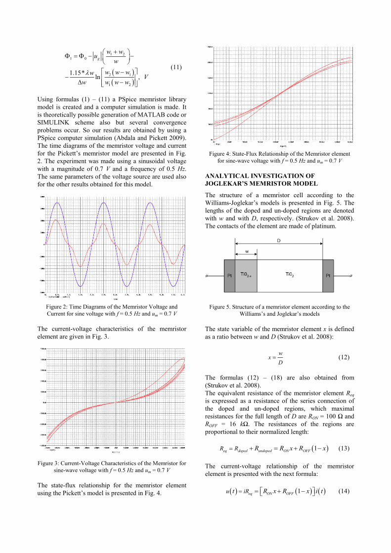
The time diagrams of the memristor voltage and current

for the Pickett’s memristor model are presented in Fig.

2. The experiment was made using a sinusoidal voltage

with a magnitude of 0.7 V and a frequency of 0.5 Hz.

The same parameters of the voltage source are used also

for the other results obtained for this model.

Figure 2: Time Diagrams of the Memristor Voltage and

Current for sine voltage with f = 0.5 Hz and um = 0.7 V

The current-voltage characteristics of the memristor

element are given in Fig. 3.

Figure 3: Current-Voltage Characteristics of the Memristor for

sine-wave voltage with f = 0.5 Hz and um = 0.7 V

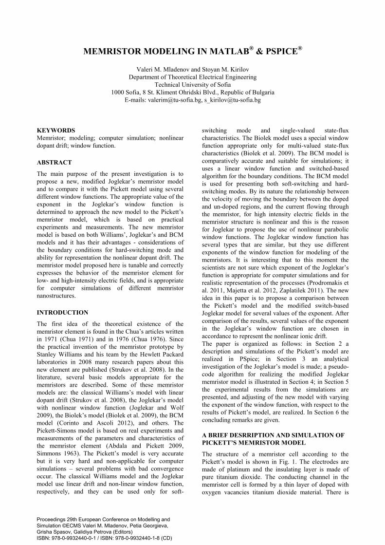
The state-flux relationship for the memristor element

using the Pickett’s model is presented in Fig. 4.

Figure 4: State-Flux Relationship of the Memristor element

for sine-wave voltage with f = 0.5 Hz and um = 0.7 V

ANALYTICAL INVESTIGATION OF

JOGLEKAR’S MEMRISTOR MODEL

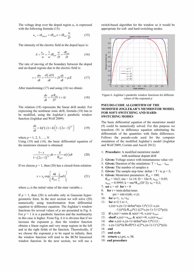
The structure of a memristor cell according to the

Williams-Joglekar’s models is presented in Fig. 5. The

lengths of the doped and un-doped regions are denoted

with w and with D, respectively. (Strukov et al. 2008).

The contacts of the element are made of platinum.

Figure 5. Structure of a memristor element according to the

Williams’s and Joglekar’s models

The state variable of the memristor element x is defined

as a ratio between w and D (Strukov et al. 2008):

w

xD

(12)

The formulas (12) – (18) are also obtained from

(Strukov et al. 2008).

The equivalent resistance of the memristor element Req

is expressed as a resistance of the series connection of

the doped and un-doped regions, which maximal

resistances for the full length of D are RON = 100 Ω and

ROFF = 16 kΩ. The resistances of the regions are

proportional to their normalized length:

1eq doped undoped ON OFFR R R R x R x (13)

The current-voltage relationship of the memristor

element is presented with the next formula:

1eq ON OFFu iRt R x R x i t (14)

The voltage drop over the doped region uw is expressed

with the following formula (15):

w doped ON ONu iRw

iR x iRD

(15)

The intensity of the electric field in the doped layer is:

1w ON

ON

uE

iRwiR

w w D D (16)

The rate of moving of the boundary between the doped

and un-doped regions due to the electric field is:

vd xDdw dx

D Edt dt dt

(17)

After transforming (17) and using (16) we obtain:

2

ONRdxi ki

dt D

(18)

The relation (18) represents the linear drift model. For

expressing the nonlinear ionic drift, formula (18) has to

be modified, using the Joglekar’s parabolic window

function (Joglekar and Wolf 2009):

2

1 2 1pdx

kif x ki xdt

(19)

where p = 1, 2, 3, …, N.

Using (19) and (14), the basic differential equation of

the memristor element is obtained:

2

1

1 2 1p

OFF

x kdx u t dt

Rx

(20)

If we choose p = 1, then (20) has a closed-form solution:

0

0

4exp

t

OFF t

kx x ud

R

(21)

where x0 is the initial value of the state variable x.

If p > 1, then (20) is solvable only in Gaussian hyper-

geometric form. In the next section we will solve (20)

numerically using transformation from differential

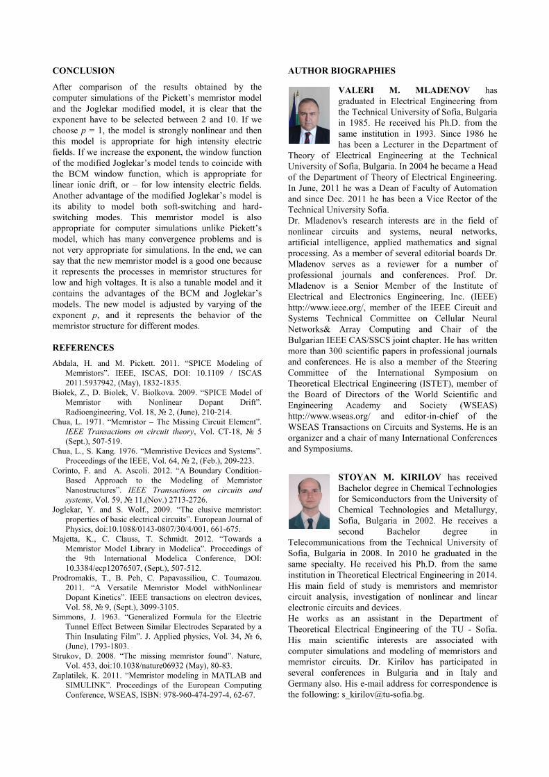
equation to difference equation. The Joglekar’s window

functions for several values of p are presented in Fig. 6.

For p = 1 it is a parabolic function and the nonlinearity

in this case is higher. From Fig. 6 it is obvious that if we

increase the exponent p, then the window function

obtains a linear region and very steep regions in the left

and in the right fields of the function. Theoretically, if

we choose the exponent p to be equal to infinity, then

the window function will tend to the BCM linearized

window function. In the next section, we will use a

switch-based algorithm for the window so it would be

appropriate for soft- and hard-switching modes.

0 0.1 0.2 0.3 0.4 0.5 0.6 0.7 0.8 0.9 10

0.1

0.2

0.3

0.4

0.5

0.6

0.7

0.8

0.9

1

State variable x

Win

dow

function f

(x)

Joglekar window functions

p = 1

p = 2

p = 10

p = 20

p = 50

Figure 6. Joglekar’s parabolic window functions for different

values of the exponent p

PSEUDO-CODE ALGORITHM OF THE

MODIFIED JOGLEKAR’S MEMRISTOR MODEL

FOR SOFT-SWITCHING AND HARD-

SWITCHING MODES

The basic differential equation of the memristor model

(9) could be numerically solved. For this purpose we

transform (9) in difference equation substituting the

differentials of the quantities with finite differences.

Follows the pseudo-code used for the computer

simulation of the modified Joglekar’s model (Joglekar

and Wolf 2009, Corinto and Ascoli 2012).

1: Procedure: A modified memristor model

with nonlinear dopant drift

2: Given: Voltage source with instantaneous value v(t)

3: Given: Duration of the simulation: T = tmax – tmin

4: Given: The number of samples n

5: Given: The sample step time: deltat = T / n; p = 5;

6: Given: Memristor parameters: Ron = 100;

Roff = 16e3; mu = 1e-14; D = 10e-9; xmin = 0.05;

xmax = 0.9999; k = mu*Ron/(D^2); x0 = 0.2;

7: set x = x0 for t = 0

8: for t = tmin:deltat:tmax

9: psi = int(v(t)dt,-∞,t);

10: for n=1, x1=x0;

11: for n=2:1:n+1,

x1(n)=x1(n-1)+deltat*u(n-1)*(1/(1-x1(n-

-1)))*(k/Roff)*(1-((2*x1(n-1)-1)^(2*p)));

12: if x1(n)<=xmin & u(n)<=0, x1(n)=xmin;

13: elseif x1(n)>=xmax & u(n)>=0, x1(n)=xmax;

14: else x1(n)=x1(n-1)+deltat*u(n-1)*(1/(1-

15: x1(n-1)))*(k/Roff)*(1-((2*x1(n-1)-1)^(2*p)));

16 end

17: end cycle

18: return u,i,psi, x, M;

19: end procedure

EXPERIMENTAL RESULTS FROM THE

COMPUTER SIMULATION REALIZED IN

MATLAB FOR SOFT-SWITCHING AND HARD-

SWITCHING MODES

The state-flux relationships of the modified Joglekar’s

memristor model for several different values of the

exponent p are given in Fig. 7. It is evident that when

the exponent p is from 1 to 10, the characteristics really

differ from one to another. When p has higher values,

then the state-flux relations almost coincide to each

other. This phenomenon is also valid for the current-

voltage relationships which are obtained for the same

conditions. The current-voltage relationships of the

memristor are illustrated in Fig. 8. Both the state-flux

and the current-voltage relationships are obtained for the

so called soft-switching mode. For this mode the values

of magnitude and frequency of voltage are the same as

these used for simulation of Pickett’s model.

-0.15 -0.1 -0.05 0 0.05 0.1 0.15 0.2 0.25 0.3 0.350.1

0.15

0.2

0.25

0.3

0.35

0.4

0.45

0.5

0.55

0.6

Flux linkage, [Wb]

Sta

te v

ariable

x

State-flux relationships for modified Joglekar model for different "p"

p = 1

p = 2

p = 10

p = 20

p = 50

Figure 7. State-flux relationships for the modified Joglekar

memristor model for different exponents p and soft-switching

operation

-0.8 -0.6 -0.4 -0.2 0 0.2 0.4 0.6 0.8-8

-6

-4

-2

0

2

4

6

8x 10

-5

Memristor voltage, [V]

Mem

risto

r curr

ent,

[A

]

Current-voltage relations for modified J. model and different p

p = 1

p = 2

p = 10

p = 20

p = 50

Figure 8. Current-voltage characteristics of the Joglekar

modified memristor model for different exponents p and soft-

switching operation

It is interesting to compare the results obtained for the

Pickett’s memristor model and the Joglekar’s modified

model – Fig. 3, Fig. 4 and Fig. 7, Fig. 8. Obviously,

these characteristics are similar to each other.

One of the advantages of the new modified Joglekar

memristor model is the possibility for adjusting the

window function so that the model is able to represent

the processes in the memristor structure for low and high

intensities of the internal electric field. The next

paragraph illustrates the results obtained for high

magnitude voltage, for example 3 V. The state-flux

characteristics are given in Fig. 9. The current-voltage

characteristics are presented in Fig. 10, respectively.

They are both obtained for the hard-switching mode,

using high voltage and low frequency signal.

-0.5 0 0.5 1 1.50

0.2

0.4

0.6

0.8

1

1.2

1.4

Flux linkage, [Wb]

Sta

te v

ariable

x

State-flux relations for different values of p

p = 1

p = 2

p = 10

p = 20

p = 50

Figure 9. State-flux relationships for the modified Joglekar

memristor model for different exponents p and hard-switching

mode

-3 -2 -1 0 1 2 3-0.005

0

0.005

0.01

0.015

0.02

0.025

0.03

Memristor Voltage, [V]

Mem

risto

r curr

ent,

[A

]

Current-voltage relations for different p and hard-switching

p = 1

p = 2

p = 10

p = 20

p = 50

Figure 10. Current-voltage characteristics of the Joglekar

modified model for different exponents p and hard-switching

After a careful consideration we can conclude that the

new memristor model is a good-quality one because it

characterizes the processes in memristor structures for

low and high intensities of the electric field. The new

algorithm is also a tunable model – it is adjusted with

varying the exponent p. The new model correctly

reproduces the boundary conditions for soft-switching

and hard-switching modes. In other words, the new

pseudo-code presented above illustrates successfully the

behavior of memristors based on titanium dioxide. It

includes the advantages both of the BCM and Joglekar’s

memristor models.

CONCLUSION

After comparison of the results obtained by the

computer simulations of the Pickett’s memristor model

and the Joglekar modified model, it is clear that the

exponent have to be selected between 2 and 10. If we

choose p = 1, the model is strongly nonlinear and then

this model is appropriate for high intensity electric

fields. If we increase the exponent, the window function

of the modified Joglekar’s model tends to coincide with

the BCM window function, which is appropriate for

linear ionic drift, or – for low intensity electric fields.

Another advantage of the modified Joglekar’s model is

its ability to model both soft-switching and hard-

switching modes. This memristor model is also

appropriate for computer simulations unlike Pickett’s

model, which has many convergence problems and is

not very appropriate for simulations. In the end, we can

say that the new memristor model is a good one because

it represents the processes in memristor structures for

low and high voltages. It is also a tunable model and it

contains the advantages of the BCM and Joglekar’s

models. The new model is adjusted by varying of the

exponent p, and it represents the behavior of the

memristor structure for different modes.

REFERENCES

Abdala, H. and M. Pickett. 2011. “SPICE Modeling of

Memristors”. IEEE, ISCAS, DOI: 10.1109 / ISCAS

2011.5937942, (May), 1832-1835.

Biolek, Z., D. Biolek, V. Biolkova. 2009. “SPICE Model of

Memristor with Nonlinear Dopant Drift”.

Radioengineering, Vol. 18, 2, (June), 210-214.

Chua, L. 1971. “Memristor – The Missing Circuit Element”.

IEEE Transactions on circuit theory, Vol. CT-18, 5

(Sept.), 507-519.

Chua, L., S. Kang. 1976. “Memristive Devices and Systems”.

Proceedings of the IEEE, Vol. 64, 2, (Feb.), 209-223.

Corinto, F. and A. Ascoli. 2012. “A Boundary Condition-

Based Approach to the Modeling of Memristor

Nanostructures”. IEEE Transactions on circuits and

systems, Vol. 59, 11,(Nov.) 2713-2726.

Joglekar, Y. and S. Wolf., 2009. “The elusive memristor:

properties of basic electrical circuits”. European Journal of

Physics, doi:10.1088/0143-0807/30/4/001, 661-675.

Majetta, K., C. Clauss, T. Schmidt. 2012. “Towards a

Memristor Model Library in Modelica”. Proceedings of

the 9th International Modelica Conference, DOI:

10.3384/ecp12076507, (Sept.), 507-512.

Prodromakis, T., B. Peh, C. Papavassiliou, C. Toumazou.

2011. “A Versatile Memristor Model withNonlinear

Dopant Kinetics”. IEEE transactions on electron devices,

Vol. 58, 9, (Sept.), 3099-3105.

Simmons, J. 1963. “Generalized Formula for the Electric

Tunnel Effect Between Similar Electrodes Separated by a

Thin Insulating Film”. J. Applied physics, Vol. 34, 6,

(June), 1793-1803.

Strukov, D. 2008. “The missing memristor found”. Nature,

Vol. 453, doi:10.1038/nature06932 (May), 80-83.

Zaplatilek, K. 2011. “Memristor modeling in MATLAB and

SIMULINK”. Proceedings of the European Computing

Conference, WSEAS, ISBN: 978-960-474-297-4, 62-67.

AUTHOR BIOGRAPHIES

VALERI M. MLADENOV has

graduated in Electrical Engineering from

the Technical University of Sofia, Bulgaria

in 1985. He received his Ph.D. from the

same institution in 1993. Since 1986 he

has been a Lecturer in the Department of

Theory of Electrical Engineering at the Technical

University of Sofia, Bulgaria. In 2004 he became a Head

of the Department of Theory of Electrical Engineering.

In June, 2011 he was a Dean of Faculty of Automation

and since Dec. 2011 he has been a Vice Rector of the

Technical University Sofia.

Dr. Mladenov's research interests are in the field of

nonlinear circuits and systems, neural networks,

artificial intelligence, applied mathematics and signal

processing. As a member of several editorial boards Dr.

Mladenov serves as a reviewer for a number of

professional journals and conferences. Prof. Dr.

Mladenov is a Senior Member of the Institute of

Electrical and Electronics Engineering, Inc. (IEEE)

http://www.ieee.org/, member of the IEEE Circuit and

Systems Technical Committee on Cellular Neural

Networks& Array Computing and Chair of the

Bulgarian IEEE CAS/SSCS joint chapter. He has written

more than 300 scientific papers in professional journals

and conferences. He is also a member of the Steering

Committee of the International Symposium on

Theoretical Electrical Engineering (ISTET), member of

the Board of Directors of the World Scientific and

Engineering Academy and Society (WSEAS)

http://www.wseas.org/ and editor-in-chief of the

WSEAS Transactions on Circuits and Systems. He is an

organizer and a chair of many International Conferences

and Symposiums.

STOYAN M. KIRILOV has received

Bachelor degree in Chemical Technologies

for Semiconductors from the University of

Chemical Technologies and Metallurgy,

Sofia, Bulgaria in 2002. He receives a

second Bachelor degree in

Telecommunications from the Technical University of

Sofia, Bulgaria in 2008. In 2010 he graduated in the

same specialty. He received his Ph.D. from the same

institution in Theoretical Electrical Engineering in 2014.

His main field of study is memristors and memristor

circuit analysis, investigation of nonlinear and linear

electronic circuits and devices.

He works as an assistant in the Department of

Theoretical Electrical Engineering of the TU - Sofia.

His main scientific interests are associated with

computer simulations and modeling of memristors and

memristor circuits. Dr. Kirilov has participated in

several conferences in Bulgaria and in Italy and

Germany also. His e-mail address for correspondence is

the following: s_kirilov@tu-sofia.bg.