matlab programming - ntnufolk.ntnu.no/thz/matlab/recktenwald/matlab week 2.pdf · matlab...
TRANSCRIPT
Matlab Programming
Gerald W. Recktenwald
Department of Mechanical Engineering
Portland State University
These slides are a supplement to the book Numerical Methods withMatlab: Implementations and Applications, by Gerald W. Recktenwald,c© 2000, Prentice-Hall, Upper Saddle River, NJ. These slides are c©2000 Gerald W. Recktenwald. The PDF version of these slides maybe downloaded or stored or printed only for noncommercial, educationaluse. The repackaging or sale of these slides in any form, without writtenconsent of the author, is prohibited.
The latest version of this PDF file, along with other supplemental materialfor the book, can be found at www.prenhall.com/recktenwald.
Version 0.96 October 5, 2000
Overview
• Script m-files
� Creating
� Side effects
• Function m-files
� Syntax of I/O parameters
� Text output
� Primary and secondary functions
• Flow control
� Relational operators
� Conditional execution of blocks
� Loops
• Vectorization
� Using vector operations instead of loops
� Preallocation of vectors and matrices
� Logical and array indexing
• Programming tricks
� Variable number of I/O parameters
� Indirect function evaluation
� Inline function objects
� Global variables
NMM: Matlab Programming page 1
Preliminaries
• Programs are contained in m-files
� Plain text files – not binary files produced by word
processors
� File must have “.m” extension
• m-file must be in the path
� Matlab maintains its own internal path
� The path is the list of directories that Matlab will search
when looking for an m-file to execute.
� A program can exist, and be free of errors, but it will not
run if Matlab cannot find it.
� Manually modify the path with the path, addpath, andrmpath built-in functions, or with addpwd NMM toolbox
function
� . . . or use interactive Path Browser
NMM: Matlab Programming page 2
Script Files
• Not really programs
� No input/output parameters
� Script variables are part of workspace
• Useful for tasks that never change
• Useful as a tool for documenting homework:
� Write a function that solves the problem for arbitrary
parameters
� Use a script to run function for specific parameters
required by the assignment
Free Advice: Scripts offer no advantage over functions.
Functions have many advantages over scripts.
Always use functions instead of scripts.
NMM: Matlab Programming page 3
Script to Plot tan(θ) (1)
Enter statements in file called tanplot.m
1. Choose New. . . from File menu
2. Enter lines listed below
Contents of tanplot.m:
theta = linspace(1.6,4.6);tandata = tan(theta);plot(theta,tandata);xlabel(’\theta (radians)’);ylabel(’tan(\theta)’);grid on;axis([min(theta) max(theta) -5 5]);
3. Choose Save. . . from File menu
Save as tanplot.m
4. Run it
>> tanplot
NMM: Matlab Programming page 4
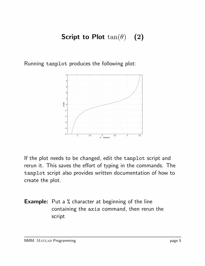
Script to Plot tan(θ) (2)
Running tanplot produces the following plot:
2 2.5 3 3.5 4 4.5-5
-4
-3
-2
-1
0
1
2
3
4
5
θ (radians)
tan(
θ)
If the plot needs to be changed, edit the tanplot script and
rerun it. This saves the effort of typing in the commands. The
tanplot script also provides written documentation of how to
create the plot.
Example: Put a % character at beginning of the line
containing the axis command, then rerun the
script
NMM: Matlab Programming page 5
Script Side-Effects (1)
All variables created in a script file are added to the workplace.
This may have undesirable effects because
• Variables already existing in the workspace may be
overwritten
• The execution of the script can be affected by the state
variables in the workspace.
Example: The easyplot script
% easyplot: Script to plot data in file xy.dat
% Load the dataD = load(’xy.dat’); % D is a matrix with two columnsx = D(:,1); y = D(:,2); % x in 1st column, y in 2nd column
plot(x,y) % Generate the plot and label itxlabel(’x axis, unknown units’)ylabel(’y axis, unknown units’)title(’Plot of generic x-y data set’)
NMM: Matlab Programming page 6
Script Side-Effects (2)
The easyplot script affects the workspace by creating three
variables:
>> clear>> who
(no variables show)>> easyplot>> who
Your variables are:
D x y
The D, x, and y variables are left in the workspace. These generic
variable names might be used in another sequence of calculations
in the same Matlab session. See Exercise 10 in Chapter 4.
NMM: Matlab Programming page 7
Script Side-Effects (3)
Side Effects, in general:
• Occur when a module changes variables other than its input
and output parameters
• Can cause bugs that are hard to track down
• Cannot always be avoided
Side Effects, from scripts
• Create and change variables in the workspace
• Give no warning that workspace variables have changed
Because scripts have side effects, it is better to encapsulate any
mildly complicated numerical in a function m-file
NMM: Matlab Programming page 8
Function m-files (1)
• Functions are subprograms:
� Functions use input and output parameters to
communicate with other functions and the command
window
� Functions use local variables that exist only while the
function is executing. Local variables are distinct from
variables of the same name in the workspace or in other
functions.
• Input parameters allow the same calculation procedure (same
algorithm) to be applied to different data. Thus, function
m-files are reusable.
• Functions can call other functions.
• Specific tasks can be encapsulated into functions. This
modular approach enables development of structured
solutions to complex problems.
NMM: Matlab Programming page 9
Function m-files (2)
Syntax:
The first line of a function m-file has the form:
function [outArgs] = funName(inArgs)
outArgs are enclosed in [ ]
• outArgs is a comma-separated list of variable names
• [ ] is optional if there is only one parameter
• functions with no outArgs are legal
inArgs are enclosed in ( )
• inArgs is a comma-separated list of variable names
• functions with no inArgs are legal
NMM: Matlab Programming page 10
Function Input and Output (1)
Examples: Demonstrate use of I/O arguments
• twosum.m — two inputs, no output
• threesum.m — three inputs, one output
• addmult.m — two inputs, two outputs
NMM: Matlab Programming page 11
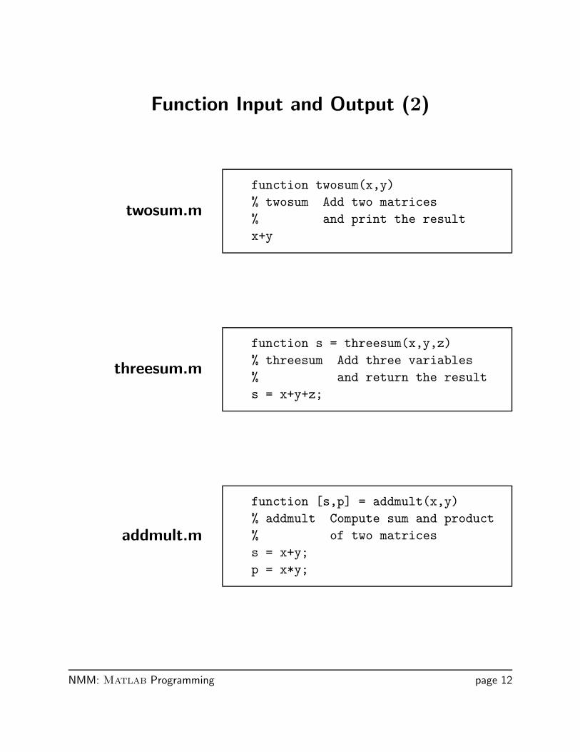
Function Input and Output (2)
twosum.m
function twosum(x,y)% twosum Add two matrices% and print the resultx+y
threesum.m
function s = threesum(x,y,z)% threesum Add three variables% and return the results = x+y+z;
addmult.m
function [s,p] = addmult(x,y)% addmult Compute sum and product% of two matricess = x+y;p = x*y;
NMM: Matlab Programming page 12
Function Input and Output Examples (3)
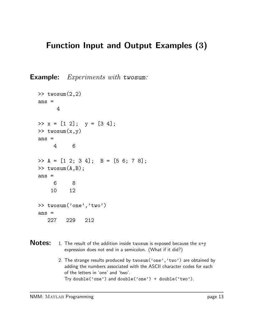
Example: Experiments with twosum:
>> twosum(2,2)ans =
4
>> x = [1 2]; y = [3 4];>> twosum(x,y)ans =
4 6
>> A = [1 2; 3 4]; B = [5 6; 7 8];>> twosum(A,B);ans =
6 810 12
>> twosum(’one’,’two’)ans =
227 229 212
Notes: 1. The result of the addition inside twosum is exposed because the x+yexpression does not end in a semicolon. (What if it did?)
2. The strange results produced by twosum(’one’,’two’) are obtained byadding the numbers associated with the ASCII character codes for eachof the letters in ‘one’ and ‘two’.Try double(’one’) and double(’one’) + double(’two’).
NMM: Matlab Programming page 13
Function Input and Output Examples (4)
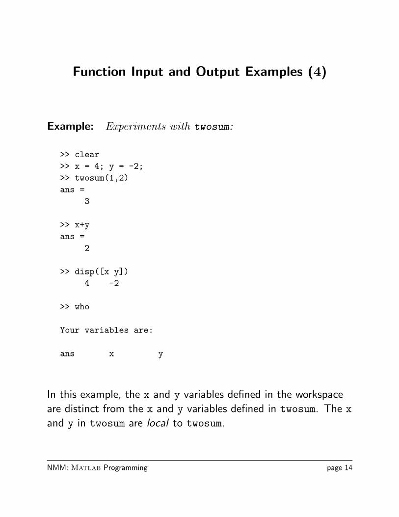
Example: Experiments with twosum:
>> clear>> x = 4; y = -2;>> twosum(1,2)ans =
3
>> x+yans =
2
>> disp([x y])4 -2
>> who
Your variables are:
ans x y
In this example, the x and y variables defined in the workspace
are distinct from the x and y variables defined in twosum. The xand y in twosum are local to twosum.
NMM: Matlab Programming page 14
Function Input and Output Examples (5)
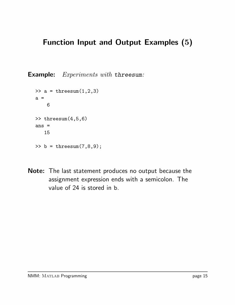
Example: Experiments with threesum:
>> a = threesum(1,2,3)a =
6
>> threesum(4,5,6)ans =
15
>> b = threesum(7,8,9);
Note: The last statement produces no output because the
assignment expression ends with a semicolon. The
value of 24 is stored in b.
NMM: Matlab Programming page 15
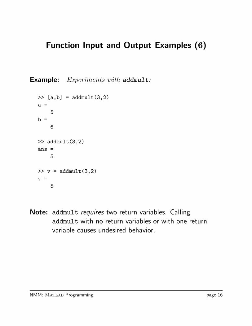
Function Input and Output Examples (6)
Example: Experiments with addmult:
>> [a,b] = addmult(3,2)a =
5b =
6
>> addmult(3,2)ans =
5
>> v = addmult(3,2)v =
5
Note: addmult requires two return variables. Calling
addmult with no return variables or with one return
variable causes undesired behavior.
NMM: Matlab Programming page 16
Summary of Input and Output Parameters
• Values are communicated through input arguments and
output arguments.
• Variables defined inside a function are local to that function.
Local variables are invisible to other functions and to the
command environment.
• The number of return variables should match the number of
output variables provided by the function. This can be
relaxed by testing for the number of return variables with
nargout (See § 3.6.1.).
NMM: Matlab Programming page 17
Text Input and Output
It is usually desirable to print results to the screen or to a file.
On rare occasions it may be helpful to prompt the user for
information not already provided by the input parameters to a
function.
Inputs to functions:
• input function can be used (and abused!).
• Input parameters to functions are preferred.
Text output from functions:
• disp function for simple output
• fprintf function for formatted output.
NMM: Matlab Programming page 18
Prompting for User Input
The input function can be used to prompt the user for numeric
or string input.
>> x = input(’Enter a value for x’);
>> yourName = input(’Enter your name’,’s’);
Prompting for input betrays the Matlab novice. It is a
nuisance to competent users, and makes automation of
computing tasks impossible.
Free Advice: Avoid using the input function. Rarely is it
necessary. All inputs to a function should be
provided via the input parameter list. Refer to
the demonstration of the inputAbuse function
in § 3.3.1.
NMM: Matlab Programming page 19
Text Output with disp and fprintf
Output to the command window is achieved with either the dispfunction or the fprintf function. Output to a file requires the
fprintf function.
disp Simple to use. Provides limited control
over appearance of output.
fprintf Slightly more complicated than disp.Provides total control over appearance
of output.
NMM: Matlab Programming page 20
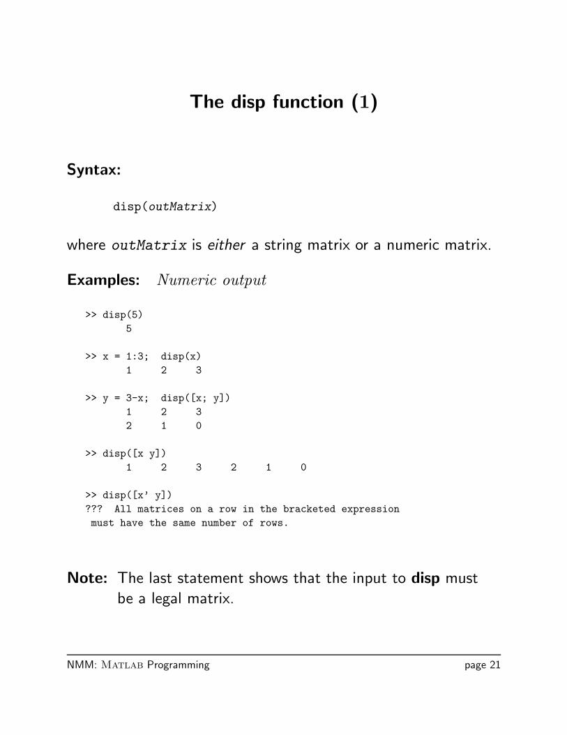
The disp function (1)
Syntax:
disp(outMatrix)
where outMatrix is either a string matrix or a numeric matrix.
Examples: Numeric output
>> disp(5)5
>> x = 1:3; disp(x)1 2 3
>> y = 3-x; disp([x; y])1 2 32 1 0
>> disp([x y])1 2 3 2 1 0
>> disp([x’ y])??? All matrices on a row in the bracketed expressionmust have the same number of rows.
Note: The last statement shows that the input to disp must
be a legal matrix.
NMM: Matlab Programming page 21
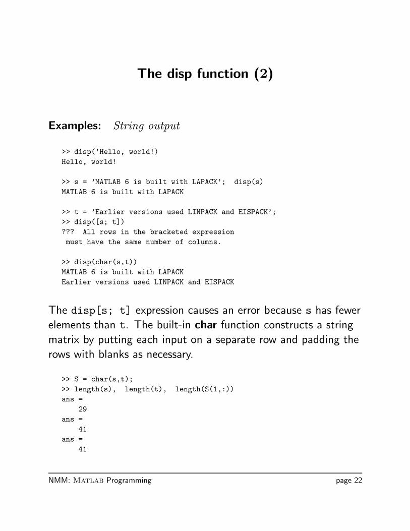
The disp function (2)
Examples: String output
>> disp(’Hello, world!)Hello, world!
>> s = ’MATLAB 6 is built with LAPACK’; disp(s)MATLAB 6 is built with LAPACK
>> t = ’Earlier versions used LINPACK and EISPACK’;>> disp([s; t])??? All rows in the bracketed expressionmust have the same number of columns.
>> disp(char(s,t))MATLAB 6 is built with LAPACKEarlier versions used LINPACK and EISPACK
The disp[s; t] expression causes an error because s has fewer
elements than t. The built-in char function constructs a string
matrix by putting each input on a separate row and padding the
rows with blanks as necessary.
>> S = char(s,t);>> length(s), length(t), length(S(1,:))ans =
29ans =
41ans =
41
NMM: Matlab Programming page 22
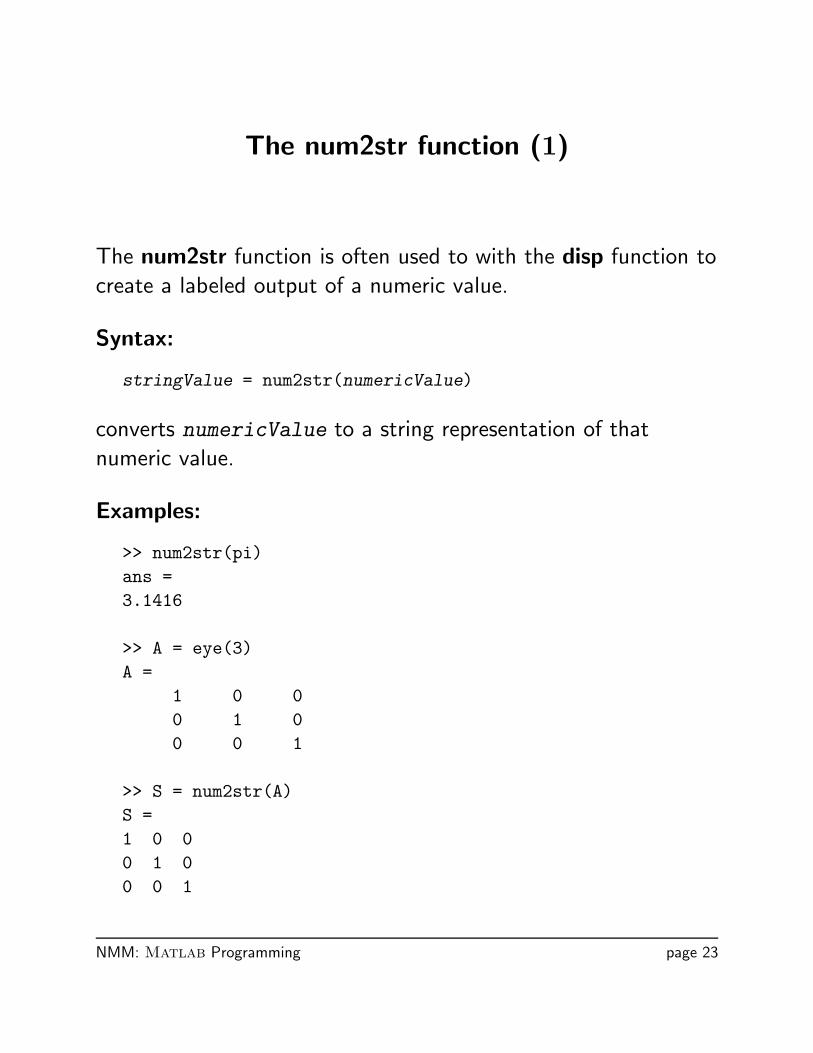
The num2str function (1)
The num2str function is often used to with the disp function to
create a labeled output of a numeric value.
Syntax:
stringValue = num2str(numericValue)
converts numericValue to a string representation of that
numeric value.
Examples:
>> num2str(pi)ans =3.1416
>> A = eye(3)A =
1 0 00 1 00 0 1
>> S = num2str(A)S =1 0 00 1 00 0 1
NMM: Matlab Programming page 23
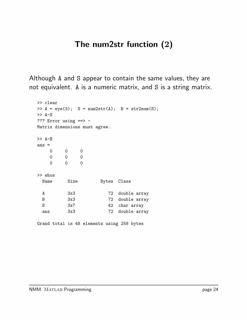
The num2str function (2)
Although A and S appear to contain the same values, they are
not equivalent. A is a numeric matrix, and S is a string matrix.
>> clear>> A = eye(3); S = num2str(A); B = str2num(S);>> A-S??? Error using ==> -Matrix dimensions must agree.
>> A-Bans =
0 0 00 0 00 0 0
>> whosName Size Bytes Class
A 3x3 72 double arrayB 3x3 72 double arrayS 3x7 42 char arrayans 3x3 72 double array
Grand total is 48 elements using 258 bytes
NMM: Matlab Programming page 24
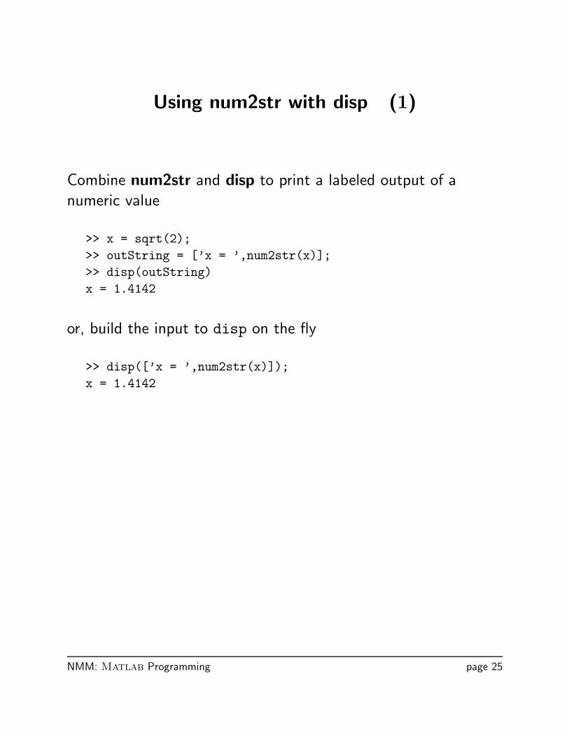
Using num2str with disp (1)
Combine num2str and disp to print a labeled output of a
numeric value
>> x = sqrt(2);>> outString = [’x = ’,num2str(x)];>> disp(outString)x = 1.4142
or, build the input to disp on the fly
>> disp([’x = ’,num2str(x)]);x = 1.4142
NMM: Matlab Programming page 25
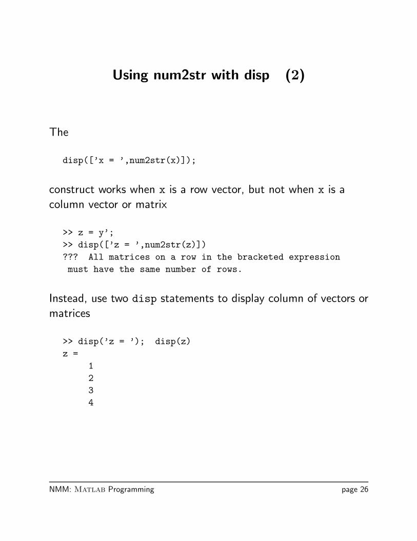
Using num2str with disp (2)
The
disp([’x = ’,num2str(x)]);
construct works when x is a row vector, but not when x is a
column vector or matrix
>> z = y’;>> disp([’z = ’,num2str(z)])??? All matrices on a row in the bracketed expressionmust have the same number of rows.
Instead, use two disp statements to display column of vectors or
matrices
>> disp(’z = ’); disp(z)z =
1234
NMM: Matlab Programming page 26
Using num2str with disp (3)
The same effect is obtained by simply entering the name of the
variable with no semicolon at the end of the line.
>> z (enter z and press return)z =
1234
NMM: Matlab Programming page 27
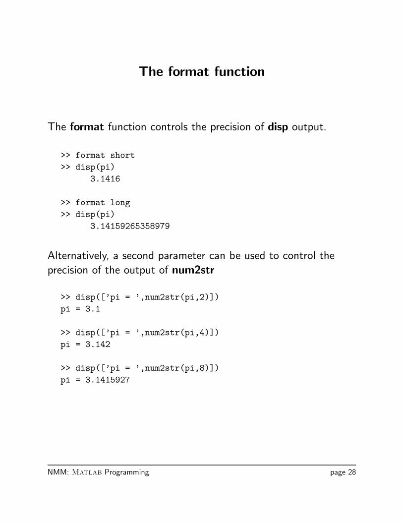
The format function
The format function controls the precision of disp output.
>> format short>> disp(pi)
3.1416
>> format long>> disp(pi)
3.14159265358979
Alternatively, a second parameter can be used to control the
precision of the output of num2str
>> disp([’pi = ’,num2str(pi,2)])pi = 3.1
>> disp([’pi = ’,num2str(pi,4)])pi = 3.142
>> disp([’pi = ’,num2str(pi,8)])pi = 3.1415927
NMM: Matlab Programming page 28
The fprintf function (1)
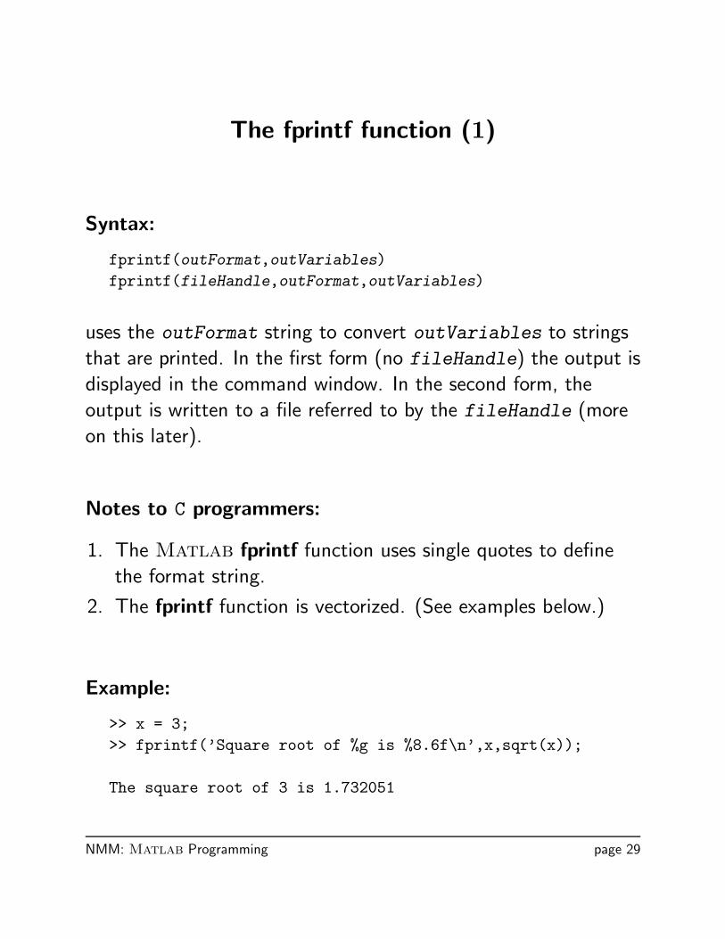
Syntax:
fprintf(outFormat,outVariables)fprintf(fileHandle,outFormat,outVariables)
uses the outFormat string to convert outVariables to strings
that are printed. In the first form (no fileHandle) the output is
displayed in the command window. In the second form, the
output is written to a file referred to by the fileHandle (more
on this later).
Notes to C programmers:
1. The Matlab fprintf function uses single quotes to define
the format string.
2. The fprintf function is vectorized. (See examples below.)
Example:
>> x = 3;>> fprintf(’Square root of %g is %8.6f\n’,x,sqrt(x));
The square root of 3 is 1.732051
NMM: Matlab Programming page 29
The fprintf function (2)
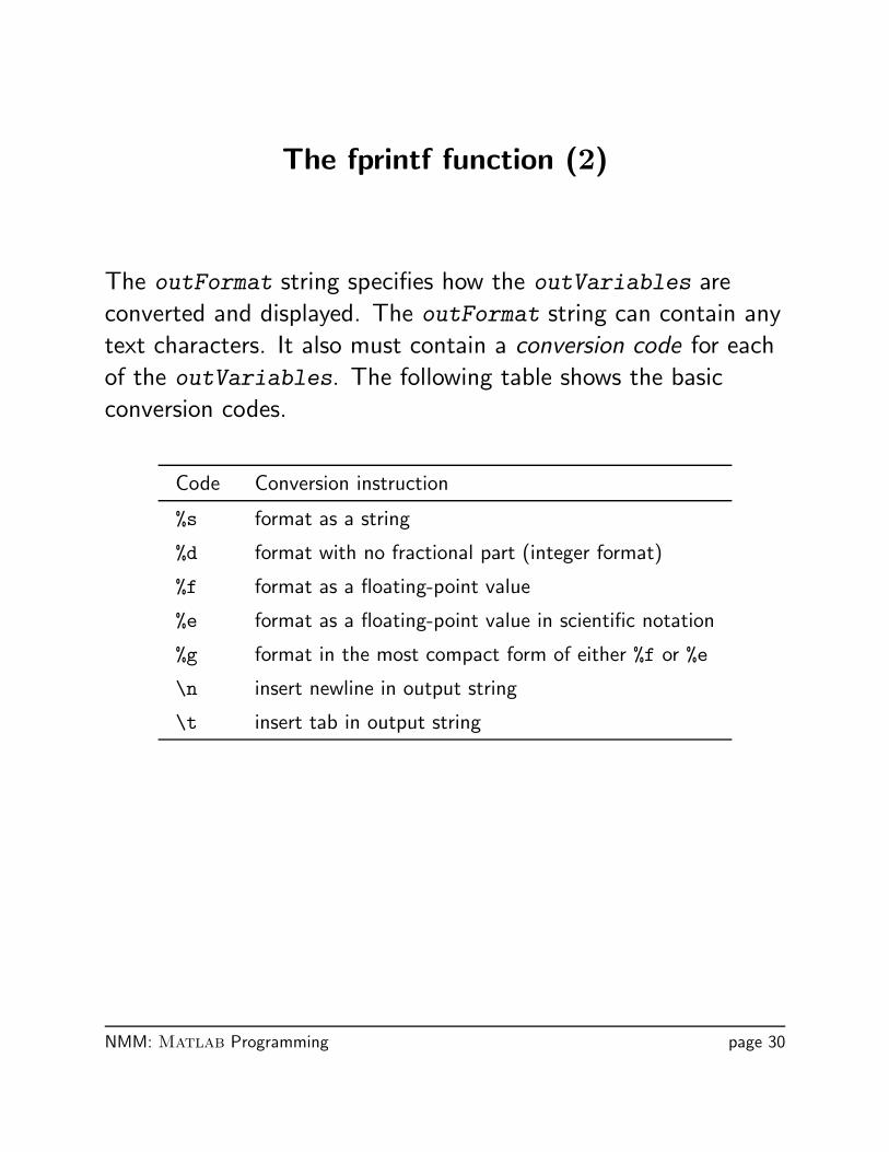
The outFormat string specifies how the outVariables are
converted and displayed. The outFormat string can contain any
text characters. It also must contain a conversion code for each
of the outVariables. The following table shows the basic
conversion codes.
Code Conversion instruction
%s format as a string
%d format with no fractional part (integer format)
%f format as a floating-point value
%e format as a floating-point value in scientific notation
%g format in the most compact form of either %f or %e
\n insert newline in output string
\t insert tab in output string
NMM: Matlab Programming page 30
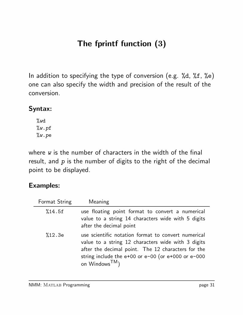
The fprintf function (3)
In addition to specifying the type of conversion (e.g. %d, %f, %e)one can also specify the width and precision of the result of the
conversion.
Syntax:
%wd%w.pf%w.pe
where w is the number of characters in the width of the final
result, and p is the number of digits to the right of the decimal
point to be displayed.
Examples:
Format String Meaning
%14.5f use floating point format to convert a numericalvalue to a string 14 characters wide with 5 digitsafter the decimal point
%12.3e use scientific notation format to convert numericalvalue to a string 12 characters wide with 3 digitsafter the decimal point. The 12 characters for thestring include the e+00 or e-00 (or e+000 or e-000
on WindowsTM)
NMM: Matlab Programming page 31
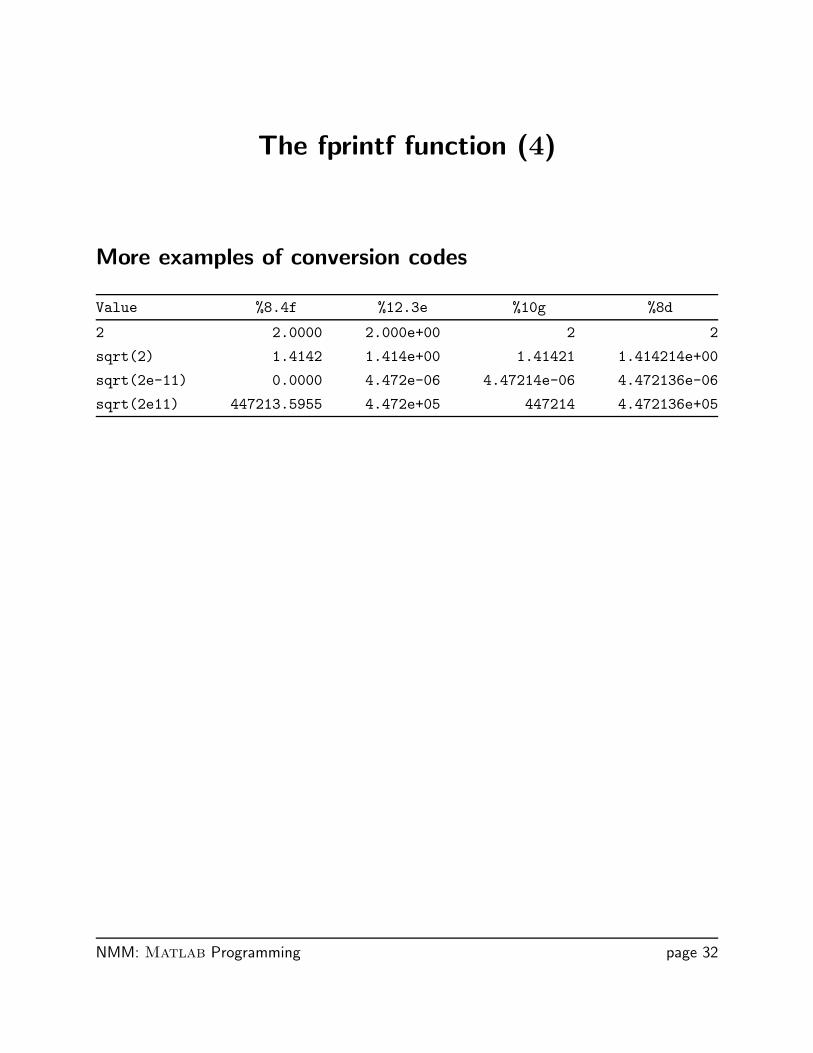
The fprintf function (4)
More examples of conversion codes
Value %8.4f %12.3e %10g %8d
2 2.0000 2.000e+00 2 2
sqrt(2) 1.4142 1.414e+00 1.41421 1.414214e+00
sqrt(2e-11) 0.0000 4.472e-06 4.47214e-06 4.472136e-06
sqrt(2e11) 447213.5955 4.472e+05 447214 4.472136e+05
NMM: Matlab Programming page 32
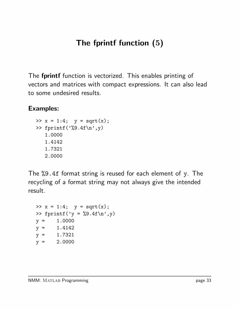
The fprintf function (5)
The fprintf function is vectorized. This enables printing of
vectors and matrices with compact expressions. It can also lead
to some undesired results.
Examples:
>> x = 1:4; y = sqrt(x);>> fprintf(’%9.4f\n’,y)
1.00001.41421.73212.0000
The %9.4f format string is reused for each element of y. Therecycling of a format string may not always give the intended
result.
>> x = 1:4; y = sqrt(x);>> fprintf(’y = %9.4f\n’,y)y = 1.0000y = 1.4142y = 1.7321y = 2.0000
NMM: Matlab Programming page 33
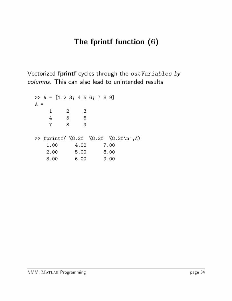
The fprintf function (6)
Vectorized fprintf cycles through the outVariables by
columns. This can also lead to unintended results
>> A = [1 2 3; 4 5 6; 7 8 9]A =
1 2 34 5 67 8 9
>> fprintf(’%8.2f %8.2f %8.2f\n’,A)1.00 4.00 7.002.00 5.00 8.003.00 6.00 9.00
NMM: Matlab Programming page 34
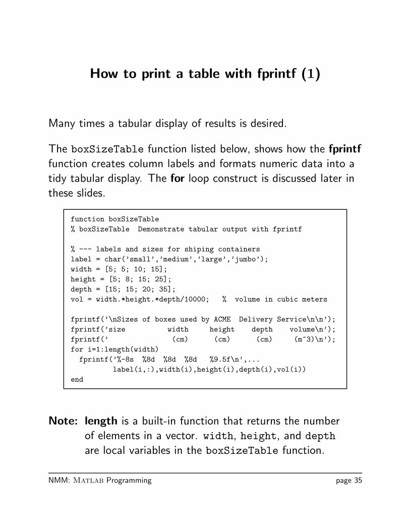
How to print a table with fprintf (1)
Many times a tabular display of results is desired.
The boxSizeTable function listed below, shows how the fprintffunction creates column labels and formats numeric data into a
tidy tabular display. The for loop construct is discussed later in
these slides.
function boxSizeTable% boxSizeTable Demonstrate tabular output with fprintf
% --- labels and sizes for shiping containerslabel = char(’small’,’medium’,’large’,’jumbo’);width = [5; 5; 10; 15];height = [5; 8; 15; 25];depth = [15; 15; 20; 35];vol = width.*height.*depth/10000; % volume in cubic meters
fprintf(’\nSizes of boxes used by ACME Delivery Service\n\n’);fprintf(’size width height depth volume\n’);fprintf(’ (cm) (cm) (cm) (m^3)\n’);for i=1:length(width)fprintf(’%-8s %8d %8d %8d %9.5f\n’,...
label(i,:),width(i),height(i),depth(i),vol(i))end
Note: length is a built-in function that returns the number
of elements in a vector. width, height, and depthare local variables in the boxSizeTable function.
NMM: Matlab Programming page 35
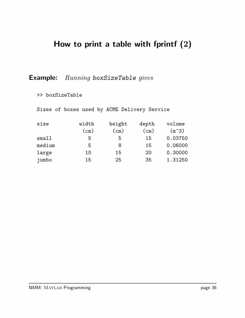
How to print a table with fprintf (2)
Example: Running boxSizeTable gives
>> boxSizeTable
Sizes of boxes used by ACME Delivery Service
size width height depth volume(cm) (cm) (cm) (m^3)
small 5 5 15 0.03750medium 5 8 15 0.06000large 10 15 20 0.30000jumbo 15 25 35 1.31250
NMM: Matlab Programming page 36
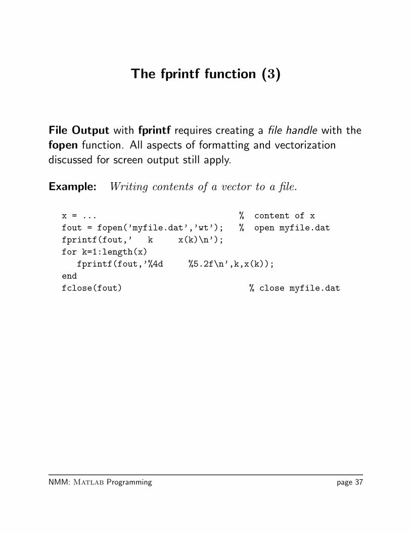
The fprintf function (3)
File Output with fprintf requires creating a file handle with the
fopen function. All aspects of formatting and vectorization
discussed for screen output still apply.
Example: Writing contents of a vector to a file.
x = ... % content of xfout = fopen(’myfile.dat’,’wt’); % open myfile.datfprintf(fout,’ k x(k)\n’);for k=1:length(x)
fprintf(fout,’%4d %5.2f\n’,k,x(k));endfclose(fout) % close myfile.dat
NMM: Matlab Programming page 37
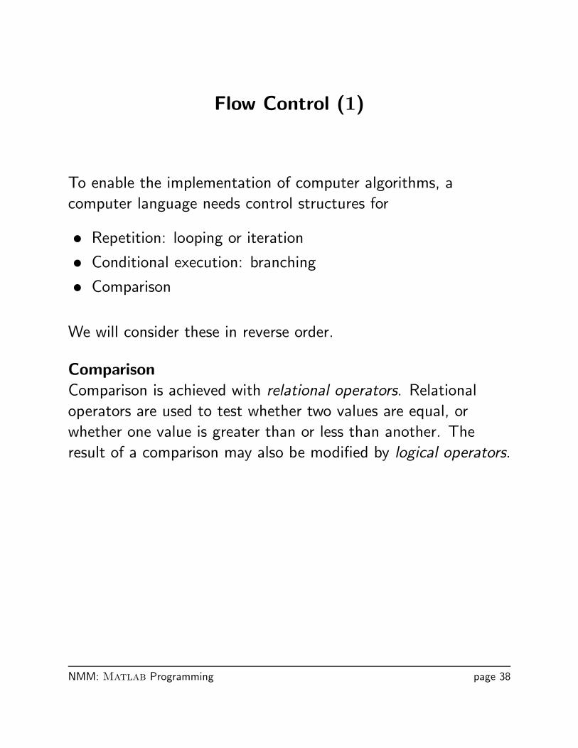
Flow Control (1)
To enable the implementation of computer algorithms, a
computer language needs control structures for
• Repetition: looping or iteration
• Conditional execution: branching
• Comparison
We will consider these in reverse order.
ComparisonComparison is achieved with relational operators. Relational
operators are used to test whether two values are equal, or
whether one value is greater than or less than another. The
result of a comparison may also be modified by logical operators.
NMM: Matlab Programming page 38
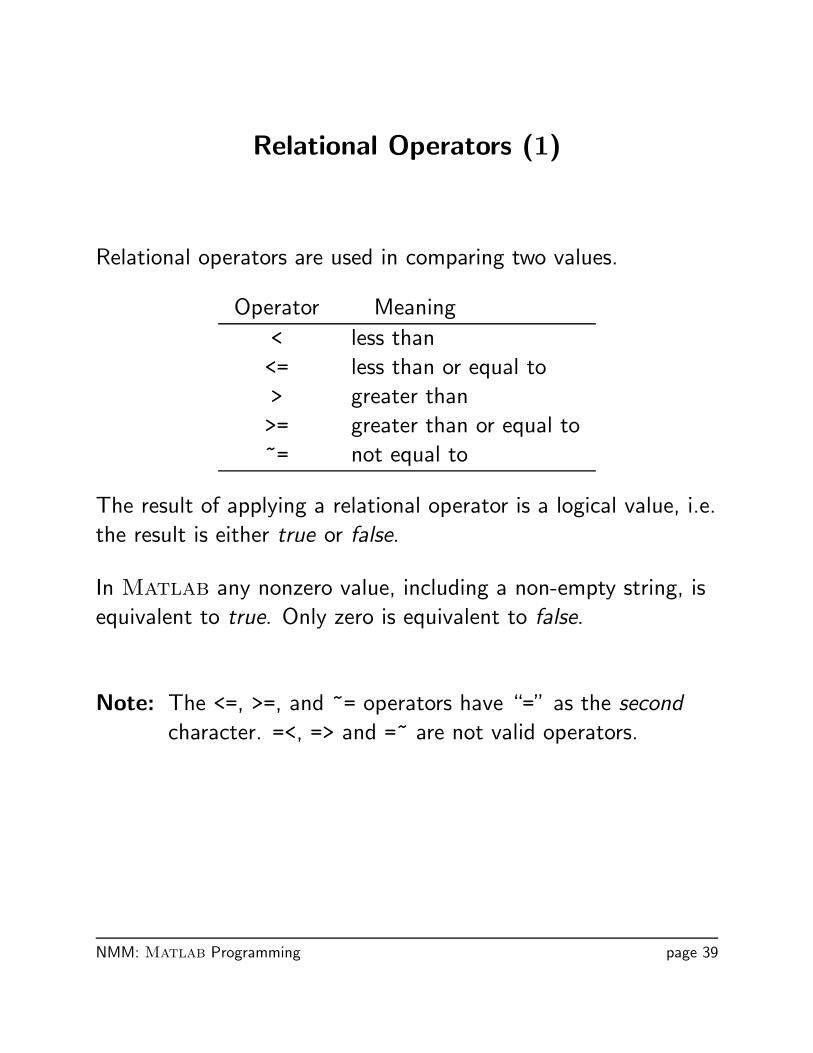
Relational Operators (1)
Relational operators are used in comparing two values.
Operator Meaning
< less than
<= less than or equal to
> greater than
>= greater than or equal to
~= not equal to
The result of applying a relational operator is a logical value, i.e.
the result is either true or false.
In Matlab any nonzero value, including a non-empty string, is
equivalent to true. Only zero is equivalent to false.
Note: The <=, >=, and ~= operators have “=” as the second
character. =<, => and =~ are not valid operators.
NMM: Matlab Programming page 39
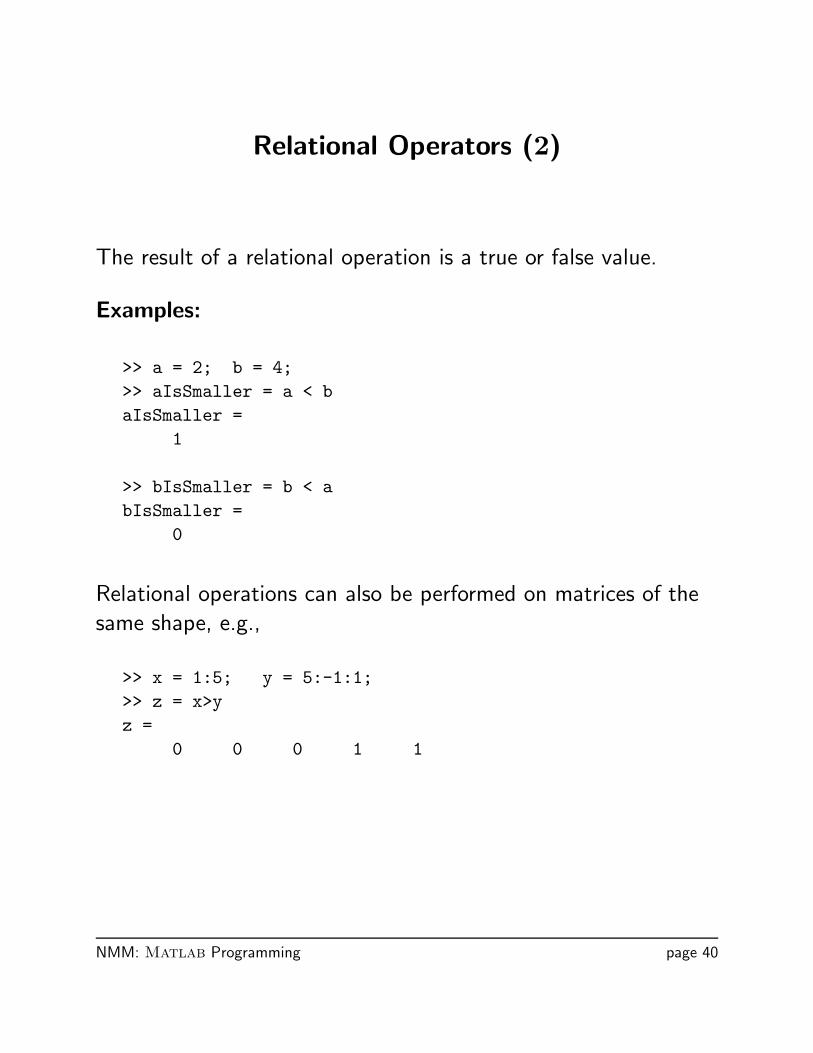
Relational Operators (2)
The result of a relational operation is a true or false value.
Examples:
>> a = 2; b = 4;>> aIsSmaller = a < baIsSmaller =
1
>> bIsSmaller = b < abIsSmaller =
0
Relational operations can also be performed on matrices of the
same shape, e.g.,
>> x = 1:5; y = 5:-1:1;>> z = x>yz =
0 0 0 1 1
NMM: Matlab Programming page 40
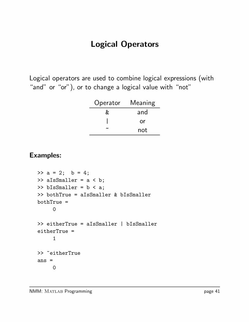
Logical Operators
Logical operators are used to combine logical expressions (with
“and” or “or”), or to change a logical value with “not”
Operator Meaning
& and
| or
~ not
Examples:
>> a = 2; b = 4;>> aIsSmaller = a < b;>> bIsSmaller = b < a;>> bothTrue = aIsSmaller & bIsSmallerbothTrue =
0
>> eitherTrue = aIsSmaller | bIsSmallereitherTrue =
1
>> ~eitherTrueans =
0
NMM: Matlab Programming page 41
Logical and Relational Operators
Summary:
• Relational operators involve comparison of two values.
• The result of a relational operation is a logical (True/False)
value.
• Logical operators combine (or negate) logical values to
produce another logical value.
• There is always more than one way to express the same
comparison
Free Advice:
• To get started, focus on simple comparison. Do not be afraid
to spread the logic over multiple lines (multiple comparisons)
if necessary.
• Try reading the test out loud.
NMM: Matlab Programming page 42
Conditional Execution
Conditional Execution or Branching:As the result of a comparison, or another logical (true/false)
test, selected blocks of program code are executed or skipped.
Conditional execution is implemented with if, if...else, andif...elseif constructs, or with a switch construct.
There are three types of if constructs
1. Plain if
2. if...else
3. if...elseif
NMM: Matlab Programming page 43
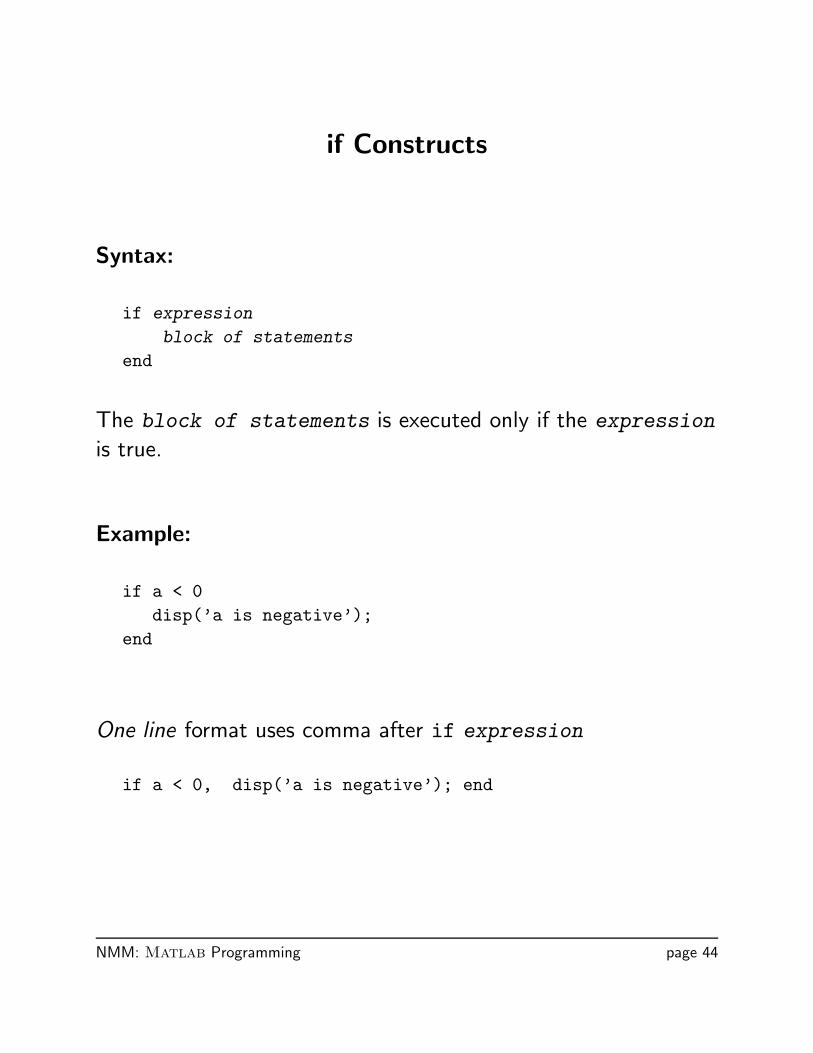
if Constructs
Syntax:
if expression
block of statements
end
The block of statements is executed only if the expression
is true.
Example:
if a < 0disp(’a is negative’);
end
One line format uses comma after if expression
if a < 0, disp(’a is negative’); end
NMM: Matlab Programming page 44
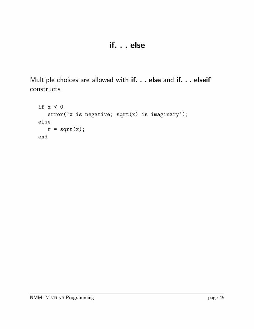
if. . . else
Multiple choices are allowed with if. . . else and if. . . elseifconstructs
if x < 0error(’x is negative; sqrt(x) is imaginary’);
elser = sqrt(x);
end
NMM: Matlab Programming page 45
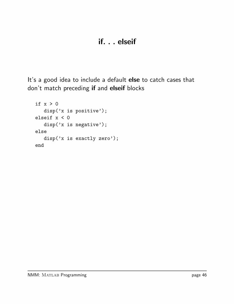
if. . . elseif
It’s a good idea to include a default else to catch cases that
don’t match preceding if and elseif blocks
if x > 0disp(’x is positive’);
elseif x < 0disp(’x is negative’);
elsedisp(’x is exactly zero’);
end
NMM: Matlab Programming page 46
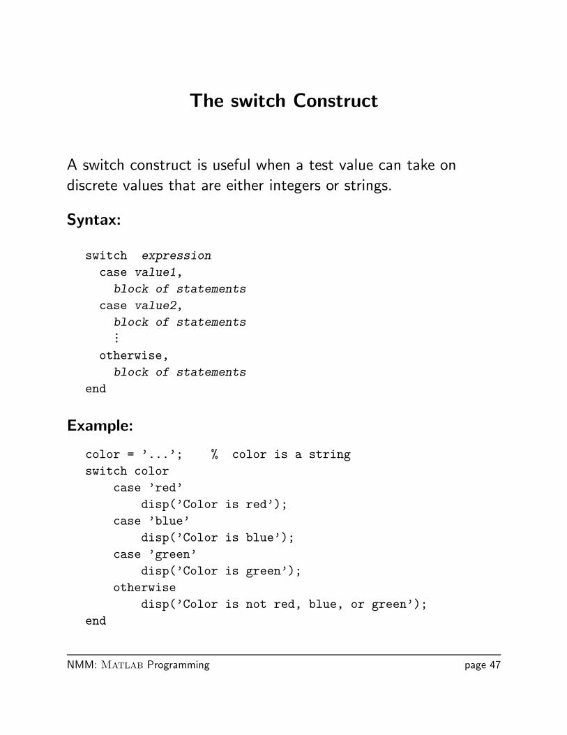
The switch Construct
A switch construct is useful when a test value can take on
discrete values that are either integers or strings.
Syntax:
switch expression
case value1,block of statements
case value2,block of statements...
otherwise,block of statements
end
Example:
color = ’...’; % color is a stringswitch color
case ’red’disp(’Color is red’);
case ’blue’disp(’Color is blue’);
case ’green’disp(’Color is green’);
otherwisedisp(’Color is not red, blue, or green’);
end
NMM: Matlab Programming page 47
Flow Control (3)
Repetition or LoopingA sequence of calculations is repeated until either
1. All elements in a vector or matrix have been processed
or
2. The calculations have produced a result that meets a
predetermined termination criterion
Looping is achieved with for loops and while loops.
NMM: Matlab Programming page 48
for loops
for loops are most often used when each element in a vector or
matrix is to be processed.
Syntax:
for index = expression
block of statements
end
Example: Sum of elements in a vector
x = 1:5; % create a row vectorsumx = 0; % initialize the sumfor k = 1:length(x)
sumx = sumx + x(k);end
NMM: Matlab Programming page 49
for loop variations
Example: A loop with an index incremented by two
for k = 1:2:n...
end
Example: A loop with an index that counts down
for k = n:-1:1...
end
Example: A loop with non-integer increments
for x = 0:pi/15:pifprintf(’%8.2f %8.5f\n’,x,sin(x));
end
Note: In the last example, x is a scalar inside the loop. Each
time through the loop, x is set equal to one of the
columns of 0:pi/15:pi.
NMM: Matlab Programming page 50
while loops (1)
while loops are most often used when an iteration is repeated
until some termination criterion is met.
Syntax:
while expression
block of statements
end
The block of statements is executed as long as expression
is true.
Example: Newton’s method for evaluating√
x
rk =1
2
(rk−1 +
x
rk−1
)
r = ... % initializerold = ...while abs(rold-r) > delta
rold = r;r = 0.5*(rold + x/rold);
end
NMM: Matlab Programming page 51
while loops (2)
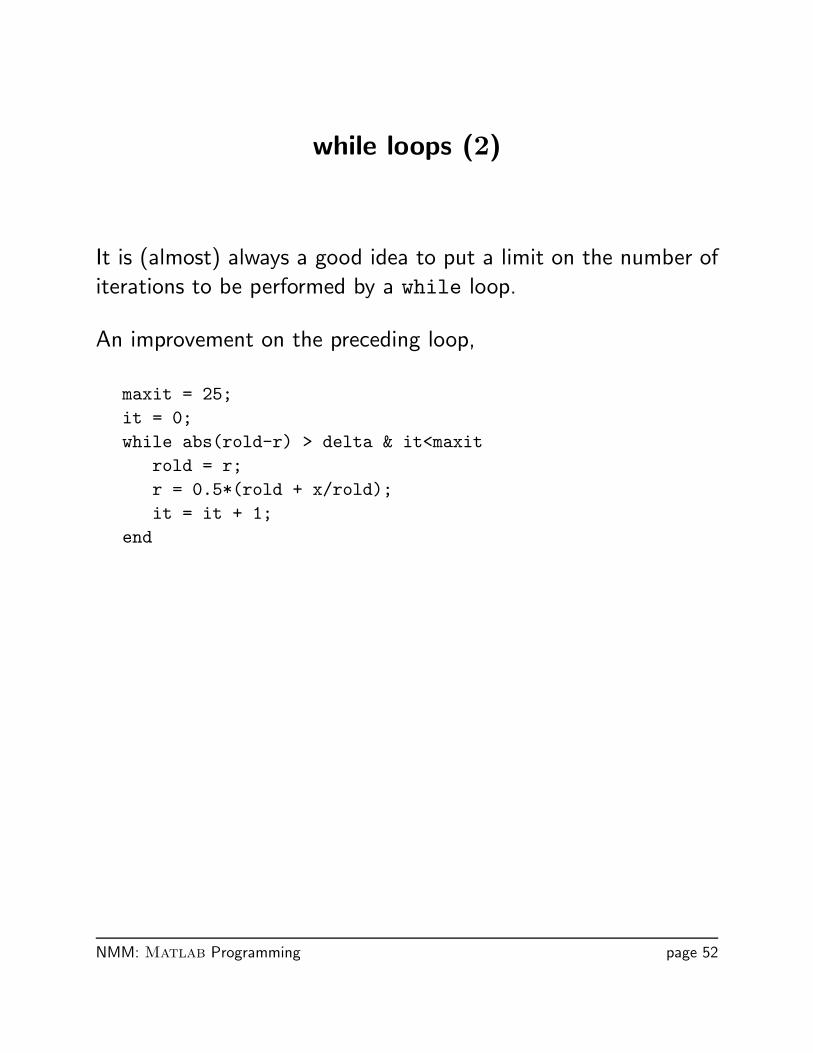
It is (almost) always a good idea to put a limit on the number of
iterations to be performed by a while loop.
An improvement on the preceding loop,
maxit = 25;it = 0;while abs(rold-r) > delta & it<maxit
rold = r;r = 0.5*(rold + x/rold);it = it + 1;
end
NMM: Matlab Programming page 52
while loops (3)
The break and return statements provide an alternative way to
exit from a loop construct. break and return may be applied to
for loops or while loops.
break is used to escape from an enclosing while or for loop.
Execution continues at the end of the enclosing loop construct.
return is used to force an exit from a function. This can have
the effect of escaping from a loop. Any statements following the
loop that are in the function body are skipped.
NMM: Matlab Programming page 53
The break command
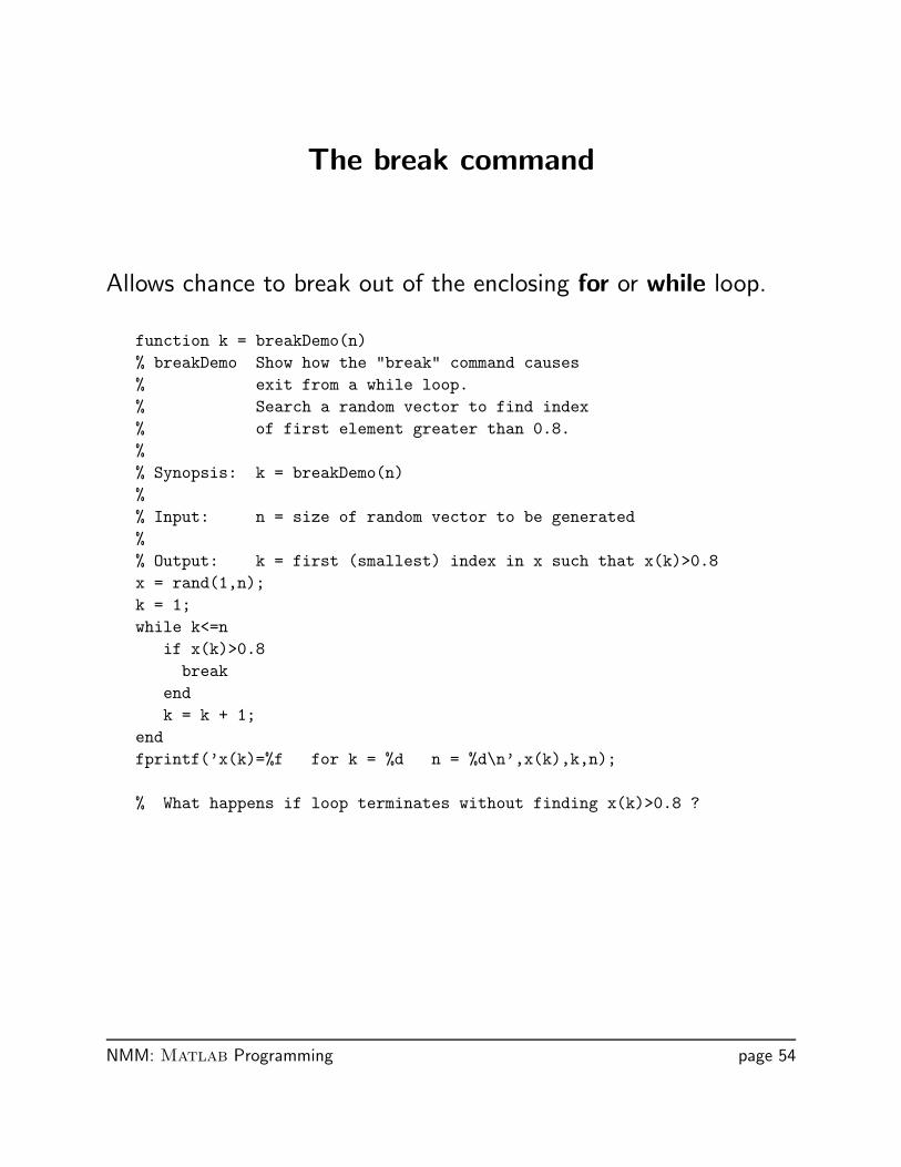
Allows chance to break out of the enclosing for or while loop.
function k = breakDemo(n)% breakDemo Show how the "break" command causes% exit from a while loop.% Search a random vector to find index% of first element greater than 0.8.%% Synopsis: k = breakDemo(n)%% Input: n = size of random vector to be generated%% Output: k = first (smallest) index in x such that x(k)>0.8x = rand(1,n);k = 1;while k<=n
if x(k)>0.8break
endk = k + 1;
endfprintf(’x(k)=%f for k = %d n = %d\n’,x(k),k,n);
% What happens if loop terminates without finding x(k)>0.8 ?
NMM: Matlab Programming page 54
The return command
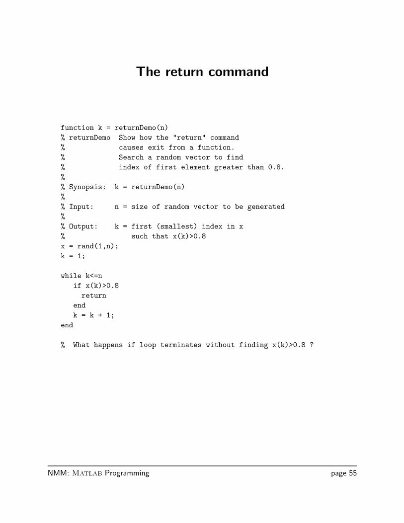
function k = returnDemo(n)% returnDemo Show how the "return" command% causes exit from a function.% Search a random vector to find% index of first element greater than 0.8.%% Synopsis: k = returnDemo(n)%% Input: n = size of random vector to be generated%% Output: k = first (smallest) index in x% such that x(k)>0.8x = rand(1,n);k = 1;
while k<=nif x(k)>0.8
returnendk = k + 1;
end
% What happens if loop terminates without finding x(k)>0.8 ?
NMM: Matlab Programming page 55
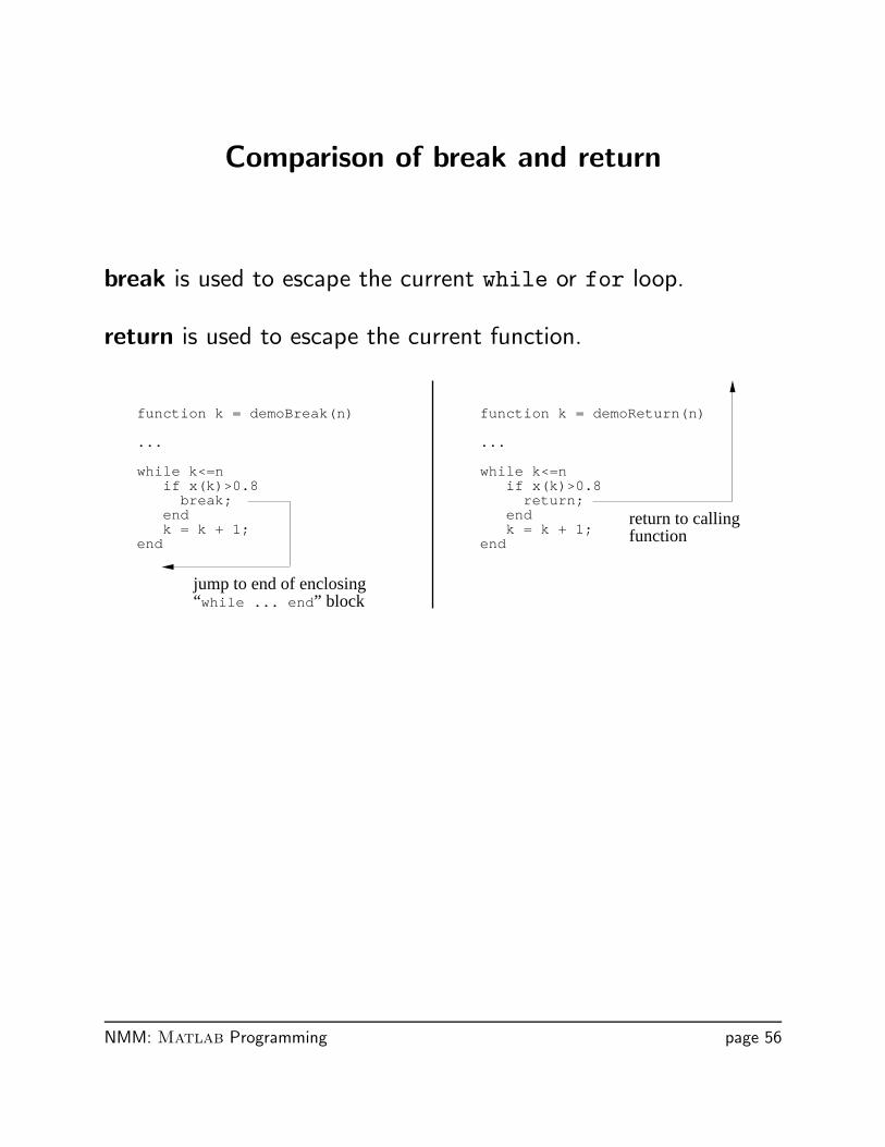
Comparison of break and return
break is used to escape the current while or for loop.
return is used to escape the current function.
function k = demoBreak(n)
...
while k<=n if x(k)>0.8 break; end k = k + 1;end
function k = demoReturn(n)
...
while k<=n if x(k)>0.8 return; end k = k + 1;end
jump to end of enclosing“while ... end” block
return to callingfunction
NMM: Matlab Programming page 56
Vectorization
Vectorization is the use of vector operations (Matlab
expressions) to process all elements of a vector or matrix.
Properly vectorized expressions are equivalent to looping over
the elements of the vectors or matrices being operated upon. A
vectorized expression is more compact and results in code that
executes faster than a non-vectorized expression.
To write vectorized code:
• Use vector operations instead of loops, where applicable
• Pre-allocate memory for vectors and matrices
• Use vectorized indexing and logical functions
Non-vectorized code is sometimes called “scalar code” because
the operations are performed on scalar elements of a vector or
matrix instead of the vector as a whole.
Free Advice: Code that is slow and correct is always better
than code that is fast and incorrect. Startwith scalar code, then vectorize as needed.
NMM: Matlab Programming page 57
Replace Loops with Vector Operations
Scalar Code
for k=1:length(x)y(k) = sin(x(k))
end
Vectorized equivalent
y = sin(x)
NMM: Matlab Programming page 58
Preallocate Memory
The following loop increases the size of s on each pass.
y = ... % some computation to define yfor j=1:length(y)
if y(j)>0s(j) = sqrt(y(j));
elses(j) = 0;
endend
Preallocate s before assigning values to elements.
y = ... % some computation to define ys = zeros(size(y));for j=1:length(y)
if y(j)>0s(j) = sqrt(y(j));
endend
NMM: Matlab Programming page 59
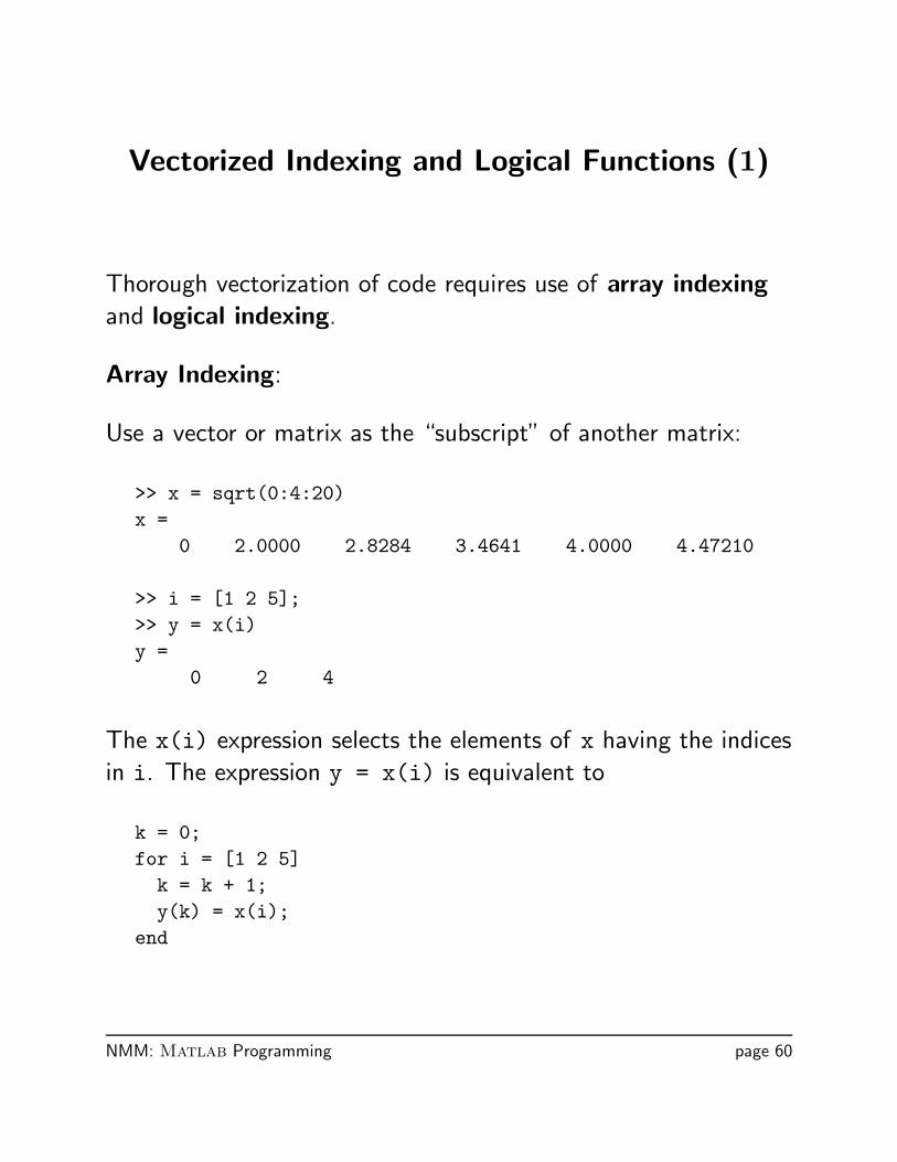
Vectorized Indexing and Logical Functions (1)
Thorough vectorization of code requires use of array indexingand logical indexing.
Array Indexing:
Use a vector or matrix as the “subscript” of another matrix:
>> x = sqrt(0:4:20)x =
0 2.0000 2.8284 3.4641 4.0000 4.47210
>> i = [1 2 5];>> y = x(i)y =
0 2 4
The x(i) expression selects the elements of x having the indices
in i. The expression y = x(i) is equivalent to
k = 0;for i = [1 2 5]
k = k + 1;y(k) = x(i);
end
NMM: Matlab Programming page 60
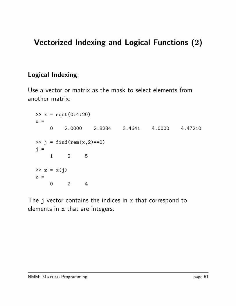
Vectorized Indexing and Logical Functions (2)
Logical Indexing:
Use a vector or matrix as the mask to select elements from
another matrix:
>> x = sqrt(0:4:20)x =
0 2.0000 2.8284 3.4641 4.0000 4.47210
>> j = find(rem(x,2)==0)j =
1 2 5
>> z = x(j)z =
0 2 4
The j vector contains the indices in x that correspond to
elements in x that are integers.
NMM: Matlab Programming page 61
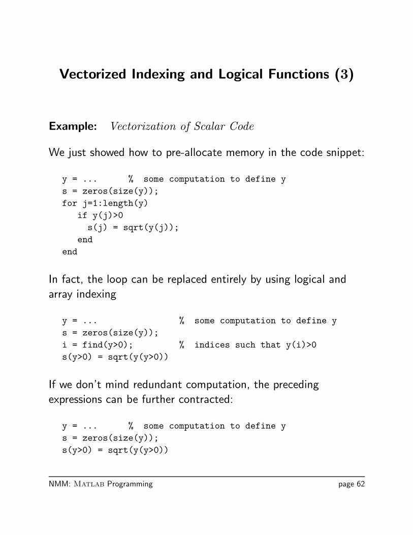
Vectorized Indexing and Logical Functions (3)
Example: Vectorization of Scalar Code
We just showed how to pre-allocate memory in the code snippet:
y = ... % some computation to define ys = zeros(size(y));for j=1:length(y)
if y(j)>0s(j) = sqrt(y(j));
endend
In fact, the loop can be replaced entirely by using logical and
array indexing
y = ... % some computation to define ys = zeros(size(y));i = find(y>0); % indices such that y(i)>0s(y>0) = sqrt(y(y>0))
If we don’t mind redundant computation, the preceding
expressions can be further contracted:
y = ... % some computation to define ys = zeros(size(y));s(y>0) = sqrt(y(y>0))
NMM: Matlab Programming page 62
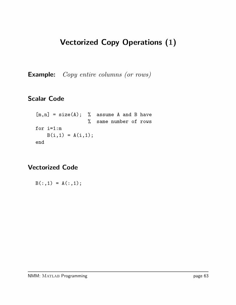
Vectorized Copy Operations (1)
Example: Copy entire columns (or rows)
Scalar Code
[m,n] = size(A); % assume A and B have% same number of rows
for i=1:mB(i,1) = A(i,1);
end
Vectorized Code
B(:,1) = A(:,1);
NMM: Matlab Programming page 63
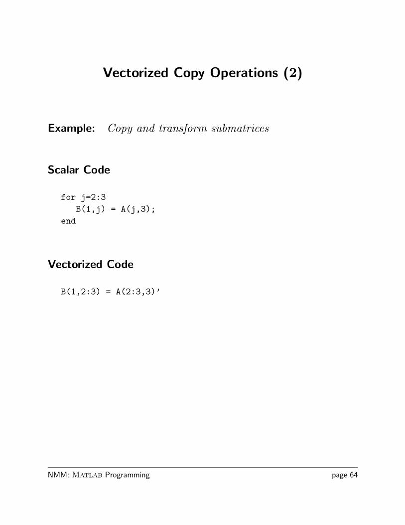
Vectorized Copy Operations (2)
Example: Copy and transform submatrices
Scalar Code
for j=2:3B(1,j) = A(j,3);
end
Vectorized Code
B(1,2:3) = A(2:3,3)’
NMM: Matlab Programming page 64
Deus ex Machina
Matlab has features to solve some recurring programming
problems:
• Variable number of I/O parameters
• Indirect function evaluation with feval
• In-line function objects (Matlab version 5.x)
• Global Variables
NMM: Matlab Programming page 65
Variable Input and Output Arguments (1)
Each function has internal variables, nargin and nargout.
Use the value of nargin at the beginning of a function to find
out how many input arguments were supplied.
Use the value of nargout at the end of a function to find out
how many input arguments are expected.
Usefulness:
• Allows a single function to perform multiple related tasks.
• Allows functions to assume default values for some inputs,
thereby simplifying the use of the function for some tasks.
NMM: Matlab Programming page 66
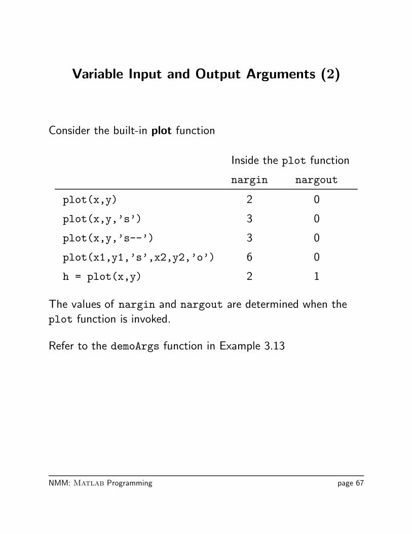
Variable Input and Output Arguments (2)
Consider the built-in plot function
Inside the plot function
nargin nargout
plot(x,y) 2 0
plot(x,y,’s’) 3 0
plot(x,y,’s--’) 3 0
plot(x1,y1,’s’,x2,y2,’o’) 6 0
h = plot(x,y) 2 1
The values of nargin and nargout are determined when the
plot function is invoked.
Refer to the demoArgs function in Example 3.13
NMM: Matlab Programming page 67
Indirect Function Evaluation (1)
The feval function allows a function to be evaluated indirectly.
Usefulness:
• Allows routines to be written to process an arbitrary f(x).
• Separates the reusable algorithm from the problem-specific
code.
feval is used extensively for root-finding (Chapter 6),
curve-fitting (Chapter 9), numerical quadrature (Chapter 11)
and numerical solution of initial value problems (Chapter 12).
NMM: Matlab Programming page 68
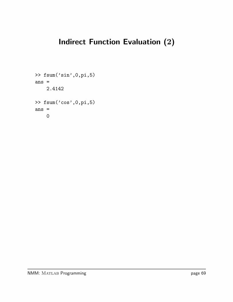
Indirect Function Evaluation (2)
>> fsum(’sin’,0,pi,5)ans =
2.4142
>> fsum(’cos’,0,pi,5)ans =
0
NMM: Matlab Programming page 69
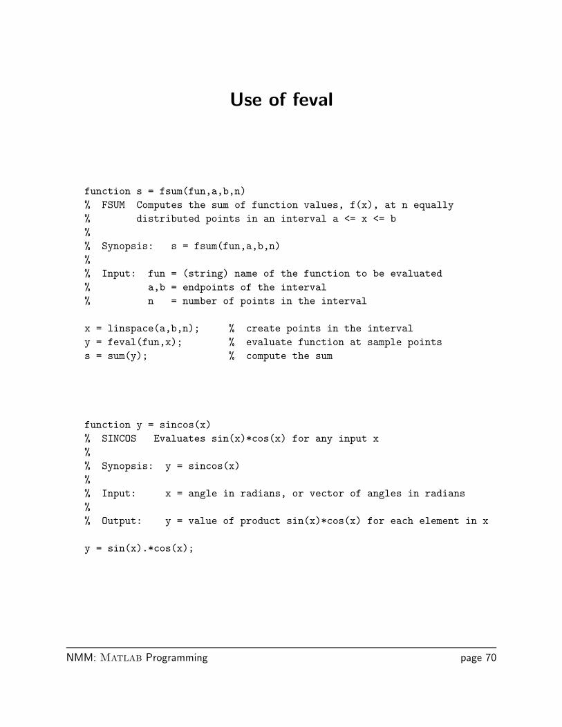
Use of feval
function s = fsum(fun,a,b,n)% FSUM Computes the sum of function values, f(x), at n equally% distributed points in an interval a <= x <= b%% Synopsis: s = fsum(fun,a,b,n)%% Input: fun = (string) name of the function to be evaluated% a,b = endpoints of the interval% n = number of points in the interval
x = linspace(a,b,n); % create points in the intervaly = feval(fun,x); % evaluate function at sample pointss = sum(y); % compute the sum
function y = sincos(x)% SINCOS Evaluates sin(x)*cos(x) for any input x%% Synopsis: y = sincos(x)%% Input: x = angle in radians, or vector of angles in radians%% Output: y = value of product sin(x)*cos(x) for each element in x
y = sin(x).*cos(x);
NMM: Matlab Programming page 70
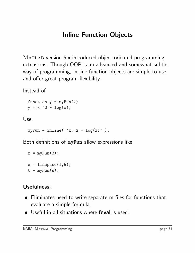
Inline Function Objects
Matlab version 5.x introduced object-oriented programming
extensions. Though OOP is an advanced and somewhat subtle
way of programming, in-line function objects are simple to use
and offer great program flexibility.
Instead of
function y = myFun(x)y = x.^2 - log(x);
Use
myFun = inline( ’x.^2 - log(x)’ );
Both definitions of myFun allow expressions like
z = myFun(3);
s = linspace(1,5);t = myFun(s);
Usefulness:
• Eliminates need to write separate m-files for functions that
evaluate a simple formula.
• Useful in all situations where feval is used.
NMM: Matlab Programming page 71
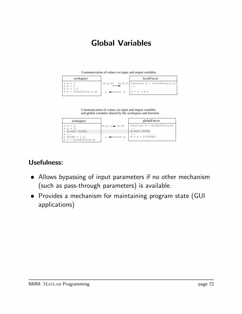
Global Variables
workspace» x = 1» y = 2» s = 1.2» z = localFun(x,y,s)
function d = localFun(a,b,c)...
d = a + b^c
localFun.m(x,y,s) (a,b,c)
z d
Communication of values via input and output variables
workspace» x = 1;» y = 2;» global ALPHA;» ...» ALPHA = 1.2;» z = globalFun(x,y)
function d = globalFun(a,b)...global ALPHA...d = a + b^ALPHA;
globalFun.m
(x,y) (a,b)
z d
Communication of values via input and output variablesand global variables shared by the workspace and function
Usefulness:
• Allows bypassing of input parameters if no other mechanism
(such as pass-through parameters) is available.
• Provides a mechanism for maintaining program state (GUI
applications)
NMM: Matlab Programming page 72