memo of freefem++ - upmc+/2016-fields/ff-memo.pdf · importantplugins qf11to25...

Memo of FreeFem++

Version 1, March 2016

F. Hecht,Laboratoire Jacques-Louis LionsUniversité Pierre et Marie Curie

Paris, France

with I. Danaila, O. Pironneau

http://www.freefem.org mailto:[email protected]

Memo, March 2016. F. Hecht et al. FreeFem++ 1 / 31

http://www.freefem.org

mailto:[email protected]

Elements of syntax: the scripts look alike C/C++ programs

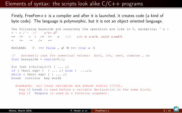
Firstly, FreeFem++ is a compiler and after it is launched, it creates code (a kind ofbyte code). The language is polymorphic, but it is not an object oriented language.

The following keywords are reserved; the operators are like in C, excepting: ^ & |+ - * / ^ // a^b= ab

== != < > <= >= & |// a|b ≡ a or b, a&b≡ a and b= += -= /= *=

BOOLEAN: 0 <=> false , 6= 0 <=> true = 1

// Automatic cast for numerical values: bool, int, reel, complex , sofunc heavyside = real(x>0.);

for (int i=0;i<n;i++) ... ;if ( <bool exp> ) ... ; else ...;;while ( <bool exp> ) ... ;break continue key words

drawback: all local variables are almost static (????),bug if break is used before a variable declaration in the same block,bug if fespace is used as a function argument.


Elements of syntax: special keywords for finite elements (FE)

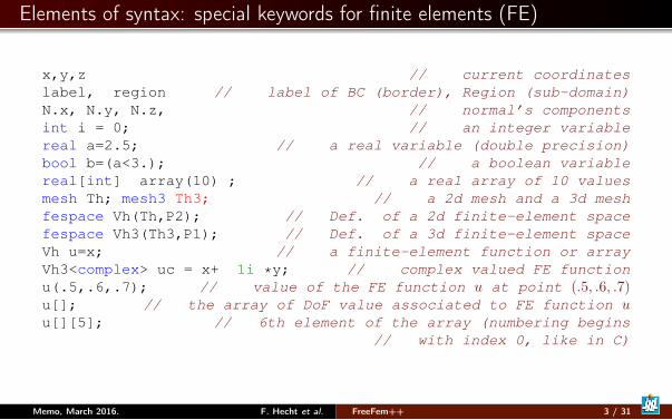
x,y,z // current coordinateslabel, region // label of BC (border), Region (sub-domain)N.x, N.y, N.z, // normal’s componentsint i = 0; // an integer variablereal a=2.5; // a real variable (double precision)bool b=(a<3.); // a boolean variablereal[int] array(10) ; // a real array of 10 valuesmesh Th; mesh3 Th3; // a 2d mesh and a 3d meshfespace Vh(Th,P2); // Def. of a 2d finite-element spacefespace Vh3(Th3,P1); // Def. of a 3d finite-element spaceVh u=x; // a finite-element function or arrayVh3<complex> uc = x+ 1i *y; // complex valued FE functionu(.5,.6,.7); // value of the FE function u at point (.5, .6, .7)u[]; // the array of DoF value associated to FE function uu[][5]; // 6th element of the array (numbering begins

// with index 0, like in C)


Elements of syntax: weak form, matrix and vector 2/4

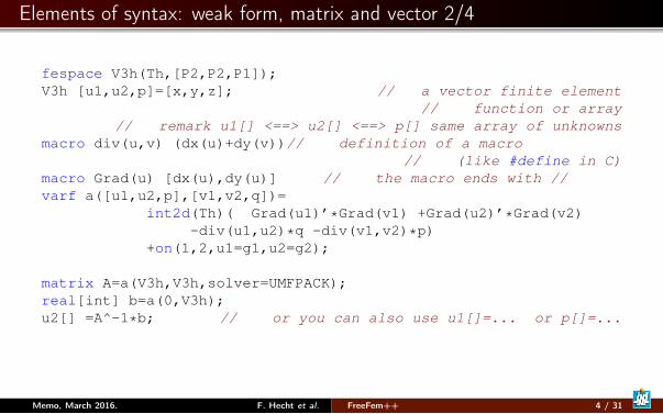
fespace V3h(Th,[P2,P2,P1]);V3h [u1,u2,p]=[x,y,z]; // a vector finite element

// function or array// remark u1[] <==> u2[] <==> p[] same array of unknowns

macro div(u,v) (dx(u)+dy(v))// definition of a macro// (like #define in C)

macro Grad(u) [dx(u),dy(u)] // the macro ends with //varf a([u1,u2,p],[v1,v2,q])=

int2d(Th)( Grad(u1)’*Grad(v1) +Grad(u2)’*Grad(v2)-div(u1,u2)*q -div(v1,v2)*p)

+on(1,2,u1=g1,u2=g2);

matrix A=a(V3h,V3h,solver=UMFPACK);real[int] b=a(0,V3h);u2[] =A^-1*b; // or you can also use u1[]=... or p[]=...


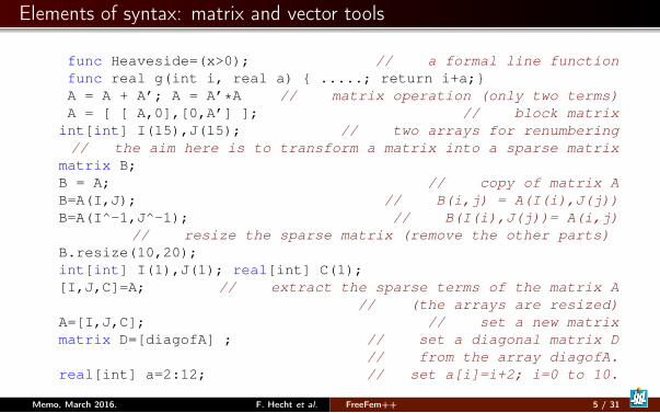
Elements of syntax: matrix and vector tools

func Heaveside=(x>0); // a formal line functionfunc real g(int i, real a) .....; return i+a;A = A + A’; A = A’*A // matrix operation (only two terms)A = [ [ A,0],[0,A’] ]; // block matrixint[int] I(15),J(15); // two arrays for renumbering// the aim here is to transform a matrix into a sparse matrix

matrix B;B = A; // copy of matrix AB=A(I,J); // B(i,j) = A(I(i),J(j))B=A(I^-1,J^-1); // B(I(i),J(j))= A(i,j)

// resize the sparse matrix (remove the other parts)B.resize(10,20);int[int] I(1),J(1); real[int] C(1);[I,J,C]=A; // extract the sparse terms of the matrix A

// (the arrays are resized)A=[I,J,C]; // set a new matrixmatrix D=[diagofA] ; // set a diagonal matrix D

// from the array diagofA.real[int] a=2:12; // set a[i]=i+2; i=0 to 10.


Elements of syntax: formal computations using arrays

a formal array is [ exp1, exp1, ..., expn]the Hermitian transposition is [ exp1, exp1, ..., expn]’

complex a=1,b=2,c=3i;func va=[ a,b,c]; // is a formal array in [ ]a =[ 1,2,3i]’*va ; cout « a « endl; // Hermitian productmatrix<complex> A=va*[ 1,2,3i]’; cout « A « endl;a =[ 1,2,3i]’*va*2.;a =(va+[ 1,2,3i])’*va*2.;va./va; // term to term /va.*va; // term to term *trace(va*[ 1,2,3i]’) ; //(va*[ 1,2,3i]’)[1][2] ; // get coefficientsdet([[1,2],[-2,1]]); // just for matrices 1x1 et 2x2

useful macros to define operators for your PDE.macro grad(u) [dx(u),dy(u)] //macro div(u1,u2) (dx(u1)+dy(u2)) // do not forget ()


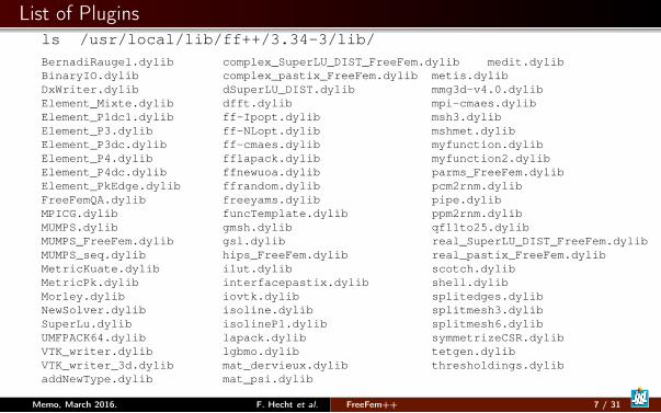
List of Pluginsls /usr/local/lib/ff++/3.34-3/lib/

BernadiRaugel.dylib complex_SuperLU_DIST_FreeFem.dylib medit.dylibBinaryIO.dylib complex_pastix_FreeFem.dylib metis.dylibDxWriter.dylib dSuperLU_DIST.dylib mmg3d-v4.0.dylibElement_Mixte.dylib dfft.dylib mpi-cmaes.dylibElement_P1dc1.dylib ff-Ipopt.dylib msh3.dylibElement_P3.dylib ff-NLopt.dylib mshmet.dylibElement_P3dc.dylib ff-cmaes.dylib myfunction.dylibElement_P4.dylib fflapack.dylib myfunction2.dylibElement_P4dc.dylib ffnewuoa.dylib parms_FreeFem.dylibElement_PkEdge.dylib ffrandom.dylib pcm2rnm.dylibFreeFemQA.dylib freeyams.dylib pipe.dylibMPICG.dylib funcTemplate.dylib ppm2rnm.dylibMUMPS.dylib gmsh.dylib qf11to25.dylibMUMPS_FreeFem.dylib gsl.dylib real_SuperLU_DIST_FreeFem.dylibMUMPS_seq.dylib hips_FreeFem.dylib real_pastix_FreeFem.dylibMetricKuate.dylib ilut.dylib scotch.dylibMetricPk.dylib interfacepastix.dylib shell.dylibMorley.dylib iovtk.dylib splitedges.dylibNewSolver.dylib isoline.dylib splitmesh3.dylibSuperLu.dylib isolineP1.dylib splitmesh6.dylibUMFPACK64.dylib lapack.dylib symmetrizeCSR.dylibVTK_writer.dylib lgbmo.dylib tetgen.dylibVTK_writer_3d.dylib mat_dervieux.dylib thresholdings.dylibaddNewType.dylib mat_psi.dylib


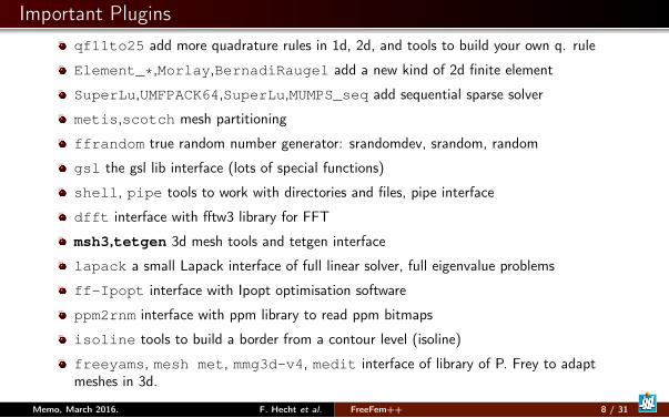
Important Pluginsqf11to25 add more quadrature rules in 1d, 2d, and tools to build your own q. rule

Element_*,Morlay,BernadiRaugel add a new kind of 2d finite element

SuperLu,UMFPACK64,SuperLu,MUMPS_seq add sequential sparse solver

metis,scotch mesh partitioning

ffrandom true random number generator: srandomdev, srandom, random

gsl the gsl lib interface (lots of special functions)

shell, pipe tools to work with directories and files, pipe interface

dfft interface with fftw3 library for FFT

msh3,tetgen 3d mesh tools and tetgen interface

lapack a small Lapack interface of full linear solver, full eigenvalue problems

ff-Ipopt interface with Ipopt optimisation software

ppm2rnm interface with ppm library to read ppm bitmaps

isoline tools to build a border from a contour level (isoline)

freeyams, mesh met, mmg3d-v4, medit interface of library of P. Frey to adaptmeshes in 3d.


Important Plugin with MPI

scharwz a new parallel linear solver (see schwarz.edp in Examples)

MUMPS a new version of MUMPS interface

MPICG parallel version of CG and GMRES

mpi-cmaes parallel version of stochastic optimization algorithm.

hips_FreeFem,parms_FreeFem,MUMPS_FreeFem old parallel linear solver iterface.


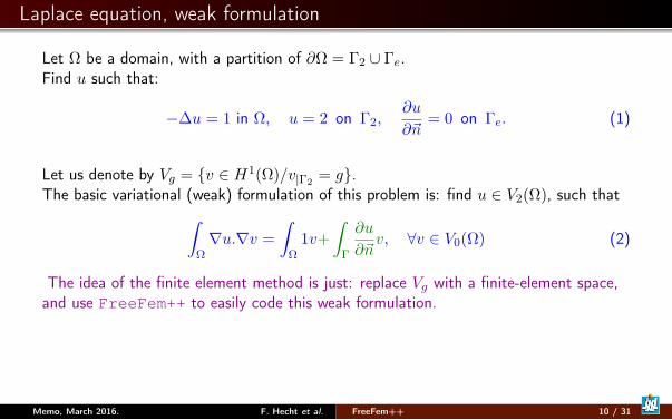
Laplace equation, weak formulation

Let Ω be a domain, with a partition of ∂Ω = Γ2 ∪ Γe.Find u such that:

−∆u = 1 in Ω, u = 2 on Γ2,∂u

∂~n= 0 on Γe. (1)

Let us denote by Vg = v ∈ H1(Ω)/v|Γ2= g.

The basic variational (weak) formulation of this problem is: find u ∈ V2(Ω), such that∫Ω∇u.∇v =

∫Ω

1v+

∫Γ

∂u

∂~nv, ∀v ∈ V0(Ω) (2)

The idea of the finite element method is just: replace Vg with a finite-element space,and use FreeFem++ to easily code this weak formulation.


Poisson equation in a fish (domain) with FreeFem++

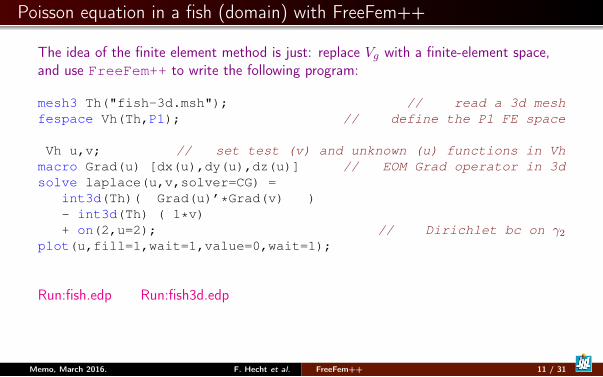
The idea of the finite element method is just: replace Vg with a finite-element space,and use FreeFem++ to write the following program:

mesh3 Th("fish-3d.msh"); // read a 3d meshfespace Vh(Th,P1); // define the P1 FE space

Vh u,v; // set test (v) and unknown (u) functions in Vhmacro Grad(u) [dx(u),dy(u),dz(u)] // EOM Grad operator in 3dsolve laplace(u,v,solver=CG) =

int3d(Th)( Grad(u)’*Grad(v) )- int3d(Th) ( 1*v)+ on(2,u=2); // Dirichlet bc on γ2

plot(u,fill=1,wait=1,value=0,wait=1);

Run:fish.edp Run:fish3d.edp


Important remarks on geometrical items: label and region instructions

All boundaries (internal or not) were defined through a label number: this numberis defined in the mesh data structure. This label number is assigned to an edge in2d and a face in 3d: FreeFem++ never uses label numbers on vertices.To define and compute an integral over a sub-domain or a boundary, you can usethe region, respectively label numbers. It is not possible to compute 1d integrals in3d domains.Presently, there are no available Finite Elements defined on a surface inFreeFem++.You can store a list of label or region numbers into an integer array (int[int]).


Remark on varf instruction

The functions appearing in the variational form are formal and local to the varf definition;the only important thing is the order in the parameter list, like in the example:varf vb1([u1,u2],[q]) = int2d(Th)( (dy(u1)+dy(u2)) *q)

+int2d(Th)(1*q) + on(1,u1=2);varf vb2([v1,v2],[p]) = int2d(Th)( (dy(v1)+dy(v2)) *p)

+int2d(Th)(1*p) ;To build the matrix from the bilinear part of the variational of type varf write simply

matrix B1 = vb1(Vh,Wh, ...);matrix<complex> C1 = vb1(Vh,Wh, ... );

// where the fespace has the correct number of components// Vh is "fespace" for the unknown fields with 2 components// ex fespace Vh(Th,[P2,P2]); or fespace Vh(Th,RT);// Wh is "fespace" for the test fields with 1 componentTo build a vector, use u1 = u2 = 0 by setting to 0 the unknown part.real[int] b = vb2(0,Wh);complex[int] c = vb2(0,Wh);

Remark: in this case the mesh used to define∫, u, v can be different.


Imposing boundary conditions

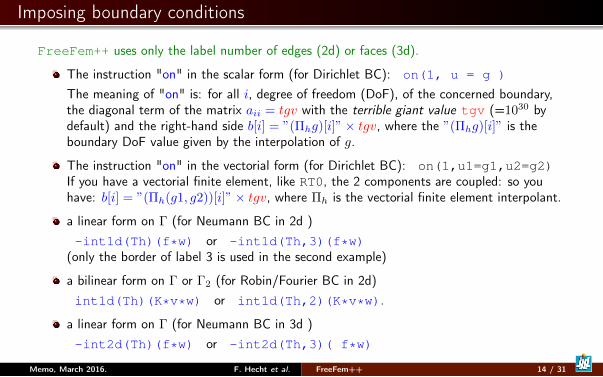
FreeFem++ uses only the label number of edges (2d) or faces (3d).

The instruction "on" in the scalar form (for Dirichlet BC): on(1, u = g )

The meaning of "on" is: for all i, degree of freedom (DoF), of the concerned boundary,the diagonal term of the matrix aii = tgv with the terrible giant value tgv (=1030 bydefault) and the right-hand side b[i] = ”(Πhg)[i]”× tgv, where the ”(Πhg)[i]” is theboundary DoF value given by the interpolation of g.

The instruction "on" in the vectorial form (for Dirichlet BC): on(1,u1=g1,u2=g2)If you have a vectorial finite element, like RT0, the 2 components are coupled: so youhave: b[i] = ”(Πh(g1, g2))[i]”× tgv, where Πh is the vectorial finite element interpolant.

a linear form on Γ (for Neumann BC in 2d )-int1d(Th)(f*w) or -int1d(Th,3)(f*w)

(only the border of label 3 is used in the second example)

a bilinear form on Γ or Γ2 (for Robin/Fourier BC in 2d)int1d(Th)(K*v*w) or int1d(Th,2)(K*v*w).

a linear form on Γ (for Neumann BC in 3d )-int2d(Th)(f*w) or -int2d(Th,3)( f*w)


Build a simple 2d Mesh

First example: generate a 10× 10 grid mesh of the unit square ]0, 1[2

int[int] labs=[10,20,30,40]; // bottom, right, top, leftmesh Th1 = square(10,10,label=labs,region=0,[x,y]); //plot(Th1,wait=1);int[int] old2newlabs=[10,11, 30,31]; // 10 -> 11, 30 -> 31Th1=change(Th1,label=old2newlabs) ; //// possible changes in 2d or 3d: region=a, fregion=f,// flabel=f

a L shape domain ]0, 1[2\[ 12 , 1[2

mesh Th = trunc(Th1,(x<0.5) | (y < 0.5),label=1);plot(Th,cmm="Th");mesh Thh = movemesh(Th,[-x,y]);mesh Th3 = Th+movemesh(Th,[-x,y]); // glue two meshesplot(Th3,cmm="Th3");

Run:mesh1.edp


Build a 2d Mesh from borders

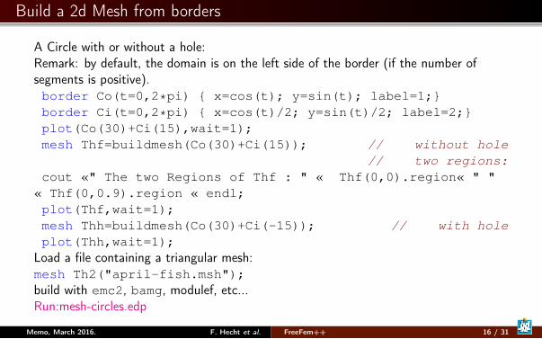
A Circle with or without a hole:Remark: by default, the domain is on the left side of the border (if the number ofsegments is positive).border Co(t=0,2*pi) x=cos(t); y=sin(t); label=1;border Ci(t=0,2*pi) x=cos(t)/2; y=sin(t)/2; label=2;plot(Co(30)+Ci(15),wait=1);mesh Thf=buildmesh(Co(30)+Ci(15)); // without hole

// two regions:cout «" The two Regions of Thf : " « Thf(0,0).region« " "

« Thf(0,0.9).region « endl;plot(Thf,wait=1);mesh Thh=buildmesh(Co(30)+Ci(-15)); // with holeplot(Thh,wait=1);

Load a file containing a triangular mesh:mesh Th2("april-fish.msh");build with emc2, bamg, modulef, etc...Run:mesh-circles.edp


Build a more complicated 2d Mesh using implicit loops

A L-shaped domain ]0, 1[2\[12 , 1[2 with 6 multi-borders.

int nn=30; real dd=0.5;real[int,int] XX=[[0,0],[1,0],[1,dd],[dd,dd],[dd,1],[0,1]];int[int] NN=[nn,nn*dd,nn*(1-dd),nn*(1-dd),nn*dd,nn];border bb(t=0,1;i) // i is the the index of the multi-border loop

int ii = (i+1)%XX.n; real t1 = 1-t;x = XX(i,0)*t1 + XX(ii,0)*t;y = XX(i,1)*t1 + XX(ii,1)*t;label = 1; ;

plot(bb(NN),wait=1);mesh Th=buildmesh(bb(NN));plot(Th,wait=1);Run:mesh-multi.edp


Build a 2d Mesh from an image 1/2

load "ppm2rnm" load "isoline" load "shell"string lac="lac-oxford", lacjpg =lac+".jpg", lacpgm =lac+".pgm";if(stat(lacpgm)<0) exec("convert "+lacjpg+" "+lacpgm);real[int,int] Curves(3,1); int[int] be(1); int nc;

real[int,int] ff1(lacpgm); // read the imageint nx = ff1.n, ny=ff1.m; // grey value in 0 to 1 (dark)mesh Th=square(nx-1,ny-1,[(nx-1)*(x),(ny-1)*(1-y)]);fespace Vh(Th,P1); Vh f1; f1[]=ff1; // array to fe function.real iso =0.3; // try some values for the level-setreal[int] viso=[iso];nc=isoline(Th,f1,iso=iso,close=0,Curves,beginend=be,

smoothing=.1,ratio=0.5);for(int i=0; i<min(3,nc);++i) int i1=be(2*i),i2=be(2*i+1)-1;

plot(f1,viso=viso,[Curves(0,i1:i2),Curves(1,i1:i2)],wait=1,cmm=i);


Build a 2d Mesh from an image 2/2

int[int] iii=[1,2]; // chose two components ...int[int] NC=[-300,-300]; // 2 componentsborder G(t=0,1;i) P=Curve(Curves,be(2*iii[i]),be(2*iii[i]+1)-1,t);

label= iii[i];plot(G(NC),wait=1);mesh Th=buildmesh(G(NC));plot(Th,wait=1);real scale = sqrt(AreaLac/Th.area);Th=movemesh(Th,[x*scale,y*scale]);Run:lac.edp (Lake Saint Jean in Quebec, Canada.)


Build a simple 3d Mesh: a cube with buildlayer

load "msh3" buildlayerint nn=10;int[int]

rup=[0,2], // label: upper face 0-> 2 (region -> label)rdown=[0,1], // label: lower face 0-> 1 (region -> label)rmid=[1,1 ,2,1 ,3,1 ,4,1 ], // 4 Vert. 2d label -> 3drtet= [0,0]; //

real zmin=0,zmax=1;mesh3 Th=buildlayers(square(nn,nn,),nn,

zbound=[zmin,zmax],region=rtet,labelmid=rmid,labelup = rup,labeldown = rdown);

Th= trunc(Th,((x<0.5) |(y< 0.5)| (z<0.5)),label=3);// remove 1/2 cube

plot("cube",Th);Run:Cube.edp


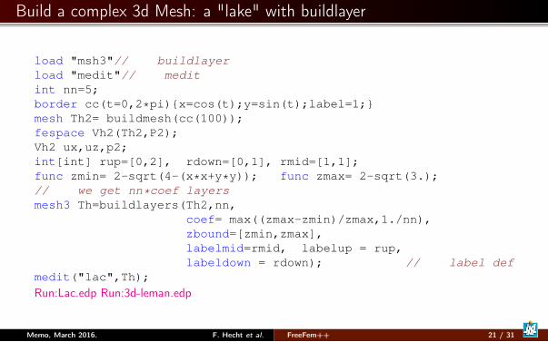
Build a complex 3d Mesh: a "lake" with buildlayer

load "msh3"// buildlayerload "medit"// meditint nn=5;border cc(t=0,2*pi)x=cos(t);y=sin(t);label=1;mesh Th2= buildmesh(cc(100));fespace Vh2(Th2,P2);Vh2 ux,uz,p2;int[int] rup=[0,2], rdown=[0,1], rmid=[1,1];func zmin= 2-sqrt(4-(x*x+y*y)); func zmax= 2-sqrt(3.);// we get nn*coef layersmesh3 Th=buildlayers(Th2,nn,

coef= max((zmax-zmin)/zmax,1./nn),zbound=[zmin,zmax],labelmid=rmid, labelup = rup,labeldown = rdown); // label def

medit("lac",Th);

Run:Lac.edp Run:3d-leman.edp


Build an axisymmetric 3d Mesh with buildlayer

func f=2*((.1+(((x/3))*(x-1)*(x-1)/1+x/100))^(1/3.)-(.1)^(1/3.));real yf=f(1.2,0);border up(t=1.2,0.) x=t;y=f;label=0;border axe2(t=0.2,1.15) x=t;y=0;label=0;border hole(t=pi,0) x= 0.15 + 0.05*cos(t);y= 0.05*sin(t);

label=1;border axe1(t=0,0.1) x=t;y=0;label=0;border queue(t=0,1) x= 1.15 + 0.05*t; y = yf*t; label =0;int np= 100;func bord= up(np)+axe1(np/10)+hole(np/10)+axe2(8*np/10)

+ queue(np/10);plot( bord); // plot the border ...mesh Th2=buildmesh(bord); // the axisymmetric 2d meshplot(Th2,wait=1);int[int] l23=[0,0,1,1];Th=buildlayers(Th2,coef= max(.15,y/max(f,0.05)), 50

,zbound=[0,2*pi],transfo=[x,y*cos(z),y*sin(z)],facemerge=1,labelmid=l23);

Run:3daximesh.edp


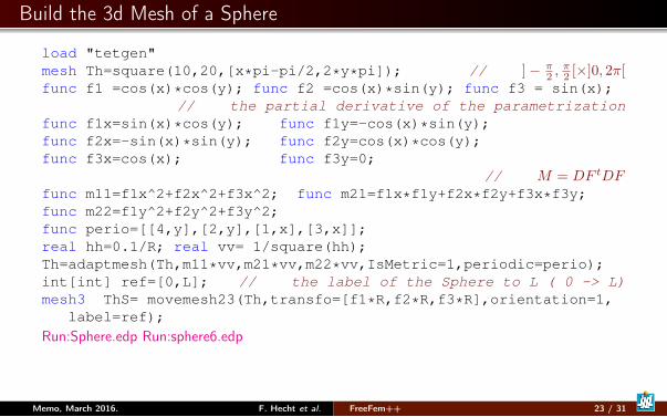
Build the 3d Mesh of a Sphere

load "tetgen"mesh Th=square(10,20,[x*pi-pi/2,2*y*pi]); // ]− π

2 ,π2 [×]0, 2π[

func f1 =cos(x)*cos(y); func f2 =cos(x)*sin(y); func f3 = sin(x);// the partial derivative of the parametrization

func f1x=sin(x)*cos(y); func f1y=-cos(x)*sin(y);func f2x=-sin(x)*sin(y); func f2y=cos(x)*cos(y);func f3x=cos(x); func f3y=0;

// M = DF tDFfunc m11=f1x^2+f2x^2+f3x^2; func m21=f1x*f1y+f2x*f2y+f3x*f3y;func m22=f1y^2+f2y^2+f3y^2;func perio=[[4,y],[2,y],[1,x],[3,x]];real hh=0.1/R; real vv= 1/square(hh);Th=adaptmesh(Th,m11*vv,m21*vv,m22*vv,IsMetric=1,periodic=perio);int[int] ref=[0,L]; // the label of the Sphere to L ( 0 -> L)mesh3 ThS= movemesh23(Th,transfo=[f1*R,f2*R,f3*R],orientation=1,

label=ref);

Run:Sphere.edp Run:sphere6.edp


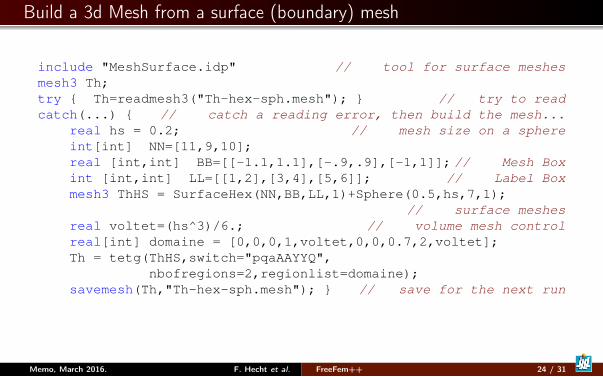
Build a 3d Mesh from a surface (boundary) mesh

include "MeshSurface.idp" // tool for surface meshesmesh3 Th;try Th=readmesh3("Th-hex-sph.mesh"); // try to readcatch(...) // catch a reading error, then build the mesh...

real hs = 0.2; // mesh size on a sphereint[int] NN=[11,9,10];real [int,int] BB=[[-1.1,1.1],[-.9,.9],[-1,1]]; // Mesh Boxint [int,int] LL=[[1,2],[3,4],[5,6]]; // Label Boxmesh3 ThHS = SurfaceHex(NN,BB,LL,1)+Sphere(0.5,hs,7,1);

// surface meshesreal voltet=(hs^3)/6.; // volume mesh controlreal[int] domaine = [0,0,0,1,voltet,0,0,0.7,2,voltet];Th = tetg(ThHS,switch="pqaAAYYQ",

nbofregions=2,regionlist=domaine);savemesh(Th,"Th-hex-sph.mesh"); // save for the next run


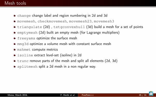
Mesh tools

change change label and region numbering in 2d and 3dmovemesh, checkmovemesh, movemesh23, movemesh3triangulate (2d) , tetgconvexhull (3d) build a mesh for a set of pointsemptymesh (2d) built an empty mesh (for Lagrange multipliers)freeyams optimize the surface meshmmg3d optimize a volume mesh with constant surface meshmshmet compute metricsisoline extract level-set (isoline) in 2dtrunc remove parts of the mesh and split all elements (2d, 3d)splitmesh split a 2d mesh in a non regular way.


Mesh adaptivity: Metrics and Unit Mesh

In Euclidean geometry the length |γ| of a curve γ of Rd parametrized by γ(t)t=0..1 is

|γ| =∫ 1

0

√< γ′(t), γ′(t) > dt

We introduce the metricM(x) as a field of d× d symmetric positive definite matrices,and the length ` of Γ w.r.tM is:

` =

∫ 1

0

√< γ′(t),M(γ(t))γ′(t) >dt

The key-idea is to construct a mesh for which the lengths of the edges are close to 1,accordingly toM.


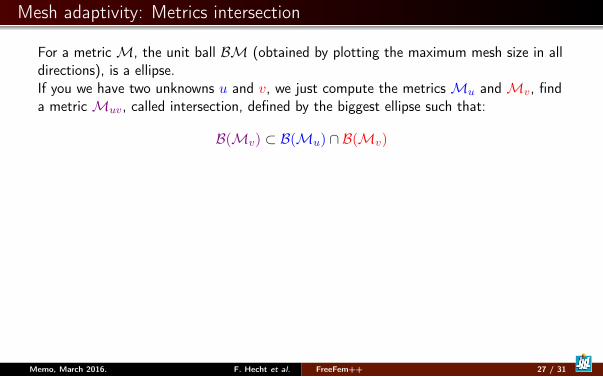
Mesh adaptivity: Metrics intersection

For a metricM, the unit ball BM (obtained by plotting the maximum mesh size in alldirections), is a ellipse.If you we have two unknowns u and v, we just compute the metricsMu andMv, finda metricMuv, called intersection, defined by the biggest ellipse such that:

B(Mv) ⊂ B(Mu) ∩ B(Mv)


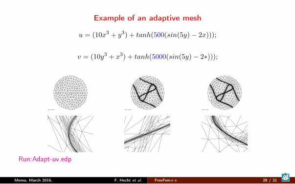
Example of an adaptive mesh

u = (10x3 + y3) + tanh(500(sin(5y)− 2x)));

v = (10y3 + x3) + tanh(5000(sin(5y)− 2∗)));

Enter ? for help Enter ? for help Enter ? for help

Run:Adapt-uv.edp


Mesh adaptivity: A corner singularity (adaptivity with metrics)

The domain is a L-shaped polygon Ω =]0, 1[2\[12 , 1]2 and the PDE is

find u ∈ H10 (Ω) such that −∆u = 1 in Ω.

The solution has a singularity at the re-entrant angle and we wish to capture itnumerically.

example of Mesh adaptation


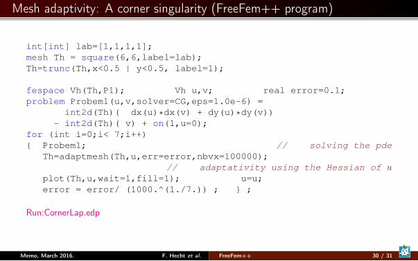
Mesh adaptivity: A corner singularity (FreeFem++ program)

int[int] lab=[1,1,1,1];mesh Th = square(6,6,label=lab);Th=trunc(Th,x<0.5 | y<0.5, label=1);

fespace Vh(Th,P1); Vh u,v; real error=0.1;problem Probem1(u,v,solver=CG,eps=1.0e-6) =

int2d(Th)( dx(u)*dx(v) + dy(u)*dy(v))- int2d(Th)( v) + on(1,u=0);

for (int i=0;i< 7;i++) Probem1; // solving the pde

Th=adaptmesh(Th,u,err=error,nbvx=100000);// adaptativity using the Hessian of u

plot(Th,u,wait=1,fill=1); u=u;error = error/ (1000.^(1./7.)) ; ;

Run:CornerLap.edp


Mesh adaptivity: building the metrics from the solution u

For P1 continuous Lagrange finite elements, the optimal metric norms for the interpolationerror (used in the function adaptmesh in FreeFem++) are:

L∞ : M =1

ε|∇∇u| = 1

ε|H|, where H = ∇∇u

Lp : M = 1ε |det(H)|

12p+2 |H|, (result by F. Alauzet, A. Dervieux)

For the norm W 1,p, the optimal metricM` for the P` Lagrange finite element is given by (withonly acute triangles) (thanks to J-M. Mirebeau)

M`,p =1

ε(detM`)

1`p+2 M`

and (see MetricPk plugin and function )

for P1: M1 = H2 (sub-optimal: for acute triangles, take H)

for P2: M2 = 3

√(a bb c

)2

+

(b cc a

)2

with

D(3)u(x, y) = (ax3 + 3bx2y + 3cxy2 + dy3)/3!,

Run:adapt.edp Run:AdaptP3.edp


memo of freefem++ - upmc+/2016-fields/ff-memo.pdf · importantplugins qf11to25...

Documents