measuring performance of exchange traded funds performance of exchange traded funds 2 measuring the...

Measuring Performanceof Exchange Traded Funds∗

Marlène HassineETF Strategy

Lyxor Asset Management, [email protected]

Thierry RoncalliResearch & Development

Lyxor Asset Management, [email protected]

February 2013

Abstract

Fund selection is an important issue for investors. This topic has spawned abundantacademic literature. Nonetheless, most of the time, these works concern only activemanagement, whereas many investors, such as institutional investors, prefer to invest inindex funds. The tools developed in the case of active management are also not suitablefor evaluating the performance of these index funds. This explains why informationratios are usually used to compare the performance of passive funds. However, weshow that this measure is not pertinent, especially when the tracking error volatility ofthe index fund is small. The objective of an exchange traded fund (ETF) is preciselyto offer an investment vehicle that presents a very low tracking error compared to itsbenchmark. In this paper, we propose a performance measure based on the value-at-riskframework, which is perfectly adapted to passive management and ETFs. Dependingon three parameters (performance difference, tracking error volatility and liquidityspread), this efficiency measure is easy to compute and may help investors in theirfund selection process. We provide some examples, and show how liquidity is more ofan issue for institutional investors than retail investors.

Keywords: Passive management, index fund, ETF, information ratio, tracking error, liq-uidity, spread, value-at-risk.

JEL classification: G11.

1 IntroductionThe market portfolio concept has a long history and dates back to the seminal work ofMarkowitz (1952). In that paper, Markowitz defines precisely what portfolio selection means:“the investor does (or should) consider expected return a desirable thing and variance of re-turn an undesirable thing”. Indeed, Markowitz shows that an efficient portfolio is a portfoliothat maximizes the expected return for a given level of risk (corresponding to the varianceof return). Markowitz concludes that there is not only one optimal portfolio, but a set ofoptimal portfolios called the efficient frontier (represented by the solid blue curve in Figure1). By studying liquidity preference, Tobin (1958) shows that the efficient frontier becomes a

∗We are profoundly grateful to Bou Ly Wu for his support with data management and the computationof liquidity spreads on limit order books. We would also like to thank Arnaud Llinas, Raphaël Dieterlen,Valérie Lalonde, François Millet and Matthieu Mouly for their helpful comments.

1

Measuring Performance of Exchange Traded Funds

straight line in the presence of a risk-free asset. If we consider a combination of an optimizedportfolio and the risk-free asset, we obtain a straight line (represented by the dashed blackline in Figure 1). But one straight line dominates all the other straight line and the efficientfrontier. It is called the Capital Market Line (CML), which corresponds to the green dashedline in Figure 1. In this case, optimal portfolios correspond to a combination of the risk-free asset and one particular efficient portfolio named the tangency portfolio. Sharpe (1964)summarizes the results of Markowitz and Tobin as follows: “the process of investment choicecan be broken down into two phases: first, the choice of a unique optimum combination ofrisky assets; and second, a separate choice concerning the allocation of funds between sucha combination and a single riskless asset”. This two-step procedure is today known as theSeparation Theorem.

One of the difficulties faced when computing the tangency portfolio is that of preciselydefining the vector of expected returns of the risky assets and the corresponding covari-ance matrix of returns. In 1964, Sharpe developed the CAPM theory and highlighted therelationship between the risk premium of the asset (the difference between the expectedreturn and the risk-free rate) and its beta (the systematic risk with respect to the tangencyportfolio). Assuming that the market is at equilibrium, he showed that the prices of assetsare such that the tangency portfolio is the market portfolio, which is composed of all riskyassets in proportion to their market capitalization. That is why we use the terms, tangencyportfolio and market portfolio indiscriminately nowadays.

Figure 1: Efficient frontier and the tangency portfolio

Another step forward was made by Jensen (1968), who measured the performance of 115(equity) mutual funds using the alpha measure and concluded that:

“The evidence on mutual fund performance indicates not only that these 115mutual funds were on average not able to predict security prices well enough to

2


outperform a buy-the-market-and-hold policy, but also that there is very littleevidence that any individual fund was able to do significantly better than thatwhich we expected from mere random chance”.

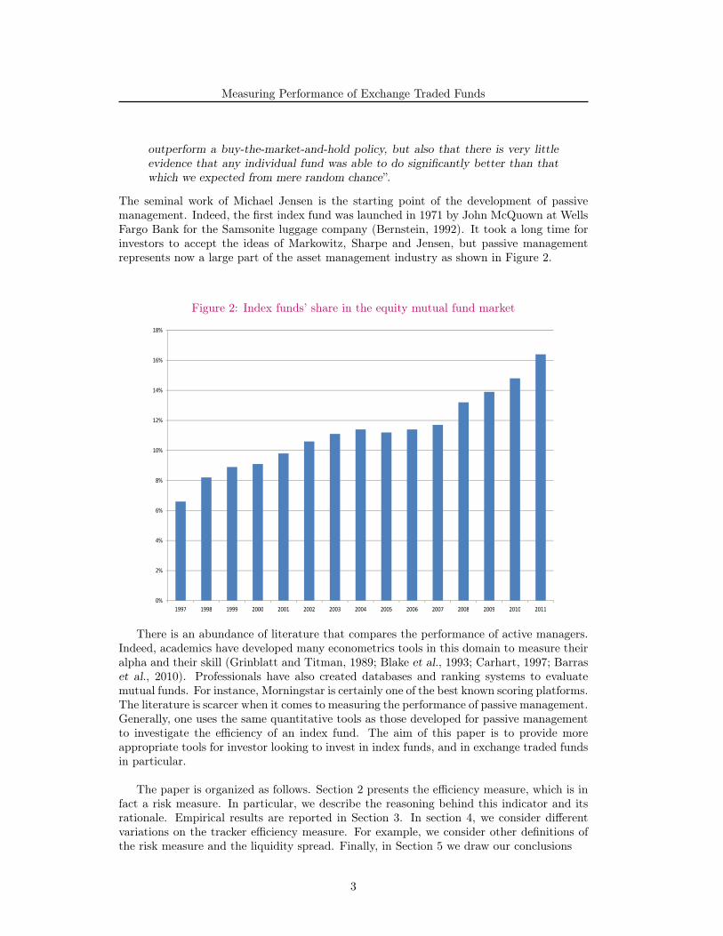
The seminal work of Michael Jensen is the starting point of the development of passivemanagement. Indeed, the first index fund was launched in 1971 by John McQuown at WellsFargo Bank for the Samsonite luggage company (Bernstein, 1992). It took a long time forinvestors to accept the ideas of Markowitz, Sharpe and Jensen, but passive managementrepresents now a large part of the asset management industry as shown in Figure 2.

Figure 2: Index funds’ share in the equity mutual fund market

16%

18%

14%

10%

12%

8%

4%

6%

2%

4%

0%

1997 1998 1999 2000 2001 2002 2003 2004 2005 2006 2007 2008 2009 2010 2011

There is an abundance of literature that compares the performance of active managers.Indeed, academics have developed many econometrics tools in this domain to measure theiralpha and their skill (Grinblatt and Titman, 1989; Blake et al., 1993; Carhart, 1997; Barraset al., 2010). Professionals have also created databases and ranking systems to evaluatemutual funds. For instance, Morningstar is certainly one of the best known scoring platforms.The literature is scarcer when it comes to measuring the performance of passive management.Generally, one uses the same quantitative tools as those developed for passive managementto investigate the efficiency of an index fund. The aim of this paper is to provide moreappropriate tools for investor looking to invest in index funds, and in exchange traded fundsin particular.

The paper is organized as follows. Section 2 presents the efficiency measure, which is infact a risk measure. In particular, we describe the reasoning behind this indicator and itsrationale. Empirical results are reported in Section 3. In section 4, we consider differentvariations on the tracker efficiency measure. For example, we consider other definitions ofthe risk measure and the liquidity spread. Finally, in Section 5 we draw our conclusions

3


2 Measuring the efficiency of exchange traded funds

2.1 Performance or efficiency measurement?

2.1.1 Understanding fund picking in active management

Fund picking could be summarized as a two-step procedures:

• Defining a universe of funds, that are sensitive to certain risk factors;

• Picking one or more elements of this universe by combining quantitative and qualitativecriteria.

The first step is crucial in order to define a universe of mutual funds, that are sufficientlyhomogeneous in terms of risk analysis. For instance, if we want to invest in equities, itcould be useful to describe the universe more accurately. Does the investment concernglobal equities, regional equities or country equities? Does the investment definition relate tospecific sectors, by focusing on or excluding some of them? What is the bias of the investmentuniverse in terms of style analysis? The capacity of the investor to clearly define the bordersof the universe is the most important part of the fund picking process, because the secondstep is relatively straightforward once the first step has been accurately completed. Forexample, investing in large capitalization equities located in the Eurozone that do not belongto the banking system, and are recognized as socially responsible, effectively reduces theuniverse to a small number of mutual funds.

Nevertheless, defining the investment universe is not always straightforward, for manyreasons. First, the category may be very large with numerous mutual funds. Suppose wewanted to invest in sovereign bonds in the Eurozone. According to the Morningstar databasethere are more than 200 such funds available. Second, a category may not necessarily existif the criteria are too specific1. Third, investment styles are heterogeneous, because theycannot be defined in a precise way. Take value and growth styles, for example. Everybodyknows what they mean, but if we ask two people to classify the components of the S&P 500index according to growth/value risk factors, we will get two different answers. This showsthat investing in active management may have a significant cost, because thorough researchis necessary to find accurate information. That is why, in the end, many investments arebased on past performance.

2.1.2 Why is fund picking different with passive management?

With passive management, fund picking is more straightforward. Indeed, the fund universeis clearly defined once the benchmark has been chosen and the problem of performanceattribution between alpha and beta components is not relevant. The investor’s goal is alsoto identify the investment vehicle that tracks the chosen index most accurately. Ratingsystems such as Morningstar and Europerformance (see Box 1) are thus not suited to thisselection challenge, because they are more concerned by absolute performance. For passivemanagers, absolute performance is meaningless. In an ideal world, they would like to buyand sell the investment at any moment and have exactly the same return as the index.Passive managers thus focus on factors other than absolute return:

1For example, an investor seeking exposure to investment grade sovereign bonds in the Eurozone, exclud-ing German bonds (because the yield is too low) and Spanish bonds (because they are too risky), wouldstruggle to find mutual funds that satisfy these criteria.

4

Measuring Performance of Exchange Traded Funds'

&

$

%

Box 1: The Europerformance/Edhec rating methodology

The ratings are constructed by combining three criteria. First, one measures extremerisks using a Cornish-Fisher value-at-risk at a 99% confidence level. If the VaR of thefund is too high, the fund is not rated. Second, the alpha of the fund is estimated. It isdone in two steps. In a first step, the style analysis of Sharpe is considered to build thecomposite benchmark of the fund. When this benchmark is selected, one deduces alphaby a regression analysis:

Rt − r = α+n∑

j=1

βj

(R

(j)t − r

)+ εt

where Rt is the return of the fund, R(j)t is the return of the ith selected benchmark and

r is the risk-free rate. The alpha criterion allows us to distinguish funds rated below andabove 3 stars. For example, the 4 and 5 stars correspond to funds which have a strictlypositive alpha. The distinction between 4 and 5 stars is done using a gain frequencymeasure. It corresponds to the number of times in percent that the fund has deliveredperformance that was better than that of its benchmark. If the gain frequency measureis less than 50%, the fund is rated 4 stars, otherwise it is rated 5 stars. Finally, a superrating is attributed to funds rated 5 stars and which have a Hurst exponent H largerthan 1/2.

1. Management fees, other costs and additional revenues;

2. Tracking error volatility;

3. Liquidity;

4. Structuration risks.

The first factor is important because it impacts on the net performance of the invest-ment vehicle. For instance, high management fees generally have a negative impact on theperformance of mutual funds. Indeed, Elton et al. (1993) investigated the informationalefficiency of mutual fund performance for the period 1964-1984 and concluded:

“There is statistically significant relationship between alpha and expenses anda relationship that can clearly be seen by examining the quintiles. Higher ex-penses are associated with poorer performance. Management does not increaseperformance by an amount sufficient that justify higher fees”.

The results are the same for index funds (Elton et al., 2004). Nevertheless, managementfees are not the only factor that impact directly on the return of an index fund. We can citefor example brokerage costs, dividend taxes, etc. A fund may also benefit from revenuesderived from securities lending, fiscal optimization or index arbitrage2.

The second factor measures the relative risk of the fund with respect to the index. Itcorresponds in general to the volatility of the tracking error, which is defined as the difference

2Index arbitrage concerns addition/deletion mechanisms of the index and corporate actions as subscrip-tion rights or optional dividend management (Dieterlen and Hereil, 2012).

5


between fund and index returns. It indicates how the tracker performance may deviate fromthe index performance. In the words of Harry Markowitz, it is ‘an undesirable thing’ forthe investor. This performance difference comes from the fact that replication strategiescannot be perfect, because the invested portfolio can not track the index weights exactlyall the time. We generally distinguish between three replication methods: full replication,optimized sampling and synthetic replication. In full replication, the fund manager invests inall index securities in the same proportion as the underlying index. But the portfolio weightscan never be identical to the theoretical index weights, unless the fund manager buys thewhole market3. Moreover, the portfolio weights are not static, as a result of subscriptionsand redemptions, dividends, cash drag, etc.

The third factor is a key element for passive funds. The liquidity of the fund is inherentlyconnected to the liquidity of the index. A S&P 500 index fund is certainly more liquid thanan MSCI emerging markets index fund. But the investment universe is not the only factorin fund liquidity. These funds are mainly bought by institutional investors, especially inEurope. Liquidity is then crucial when they carry out subscriptions or redemptions. Thesedecisions may have a big impact on the market. Moreover, the fund manager has littlemargin for discretionary decisions, because he has to follow the systematic index strategy.The index ignores more and less liquidity, but the index fund does not. Some recent events,like the March 2011 Tohoku earthquake in Japan or the Greek debt crisis, have shownhow difficult it can be to manage the liquidity of an index fund in the face of such stressscenarios. Redemptions from Japanese equity index funds were difficult to execute in thedays after the catastrophe in northern Japan on Friday March 11, 2011. In the same way,the decision of EuroMTS to keep Greek bonds in the EuroMTS Eurozone Govies index (exCNO) after Greece was downgraded from investment grade in April 2010 caused problems inmanaging index funds that were benchmarked to this index. The problem is more complexwith trackers, because they offer intra-day liquidity. And this liquidity has a cost, whichcan be measured by bid-ask spreads.

Another element that is important for investors is the operational structure of an ETF.We generally distinguish two main structures (physical and synthetic) used in the Europeanmarkets. Even if the operational structure may be sometimes an important criteria forinvestors, it is more a go/no go check test than a statistic that can be taken into account inthe design of an efficiency measure.

2.1.3 Portfolio optimization when there is a benchmark

We may think that the Markowitz approach is less relevant when there is a benchmark.However, it could easily be adapted by replacing the volatility of the portfolio by the volatilityof the tracking error. Let b (or x) be the vector of weights of the benchmark (or the activeportfolio). We note n the number of assets in the investment universe and Ri the return of

3Let us assume that the index is composed of two stocks. Let Ni,t and Pi,t be the number of outstandingshares and the price of the ith stock at time t. The index weights are given by:

wi,t =Ni,tPi,t∑2i=1 Ni,tPi,t

For example, if N1,t = 136017, N2,t = 87123, P1,t = 110.54, N2,t = 125.23, we have w1,t = 57.95% andw2,t = 42.05%. If the value of the fund is $1000, full replication involves buying respectively 5 and 3 sharesof the first and second stocks, whereas the cash represents $71.61. The portfolio weights of the two stocksare then w1,t = 55.27% and w2,t = 37.57%. At time t+ 1, we assume that there is a subscription of $60. Ifthe prices remain the same, we could buy another share of either the first stock or the second stock. In thetwo cases, we obtain portfolio weights that are different from the index weights.

6


the asset i. The tracking error of the active portfolio x with respect to the benchmark is thedifference between the return of the portfolio R (x) and the return of the benchmark R (b):

e = R (x)−R (b)

=

n∑i=1

xiRi −n∑

i=1

biRi

= x⊤R− b⊤R

= (x− b)⊤R

The expected tracking error is defined as follows:

µ (x | b) = E [e]

= (x− b)⊤µ

whereas tracking error volatility is equal to4:

σ2 (x | b) = σ2 (e)

= (x− b)⊤Σ (x− b)

The objective of the investor is to maximize the expected tracking error with a constrainton the tracking error volatility:

x⋆ = argmax (x− b)⊤µ

u.c. 1⊤x = 1 and σ (e) ≤ σ⋆

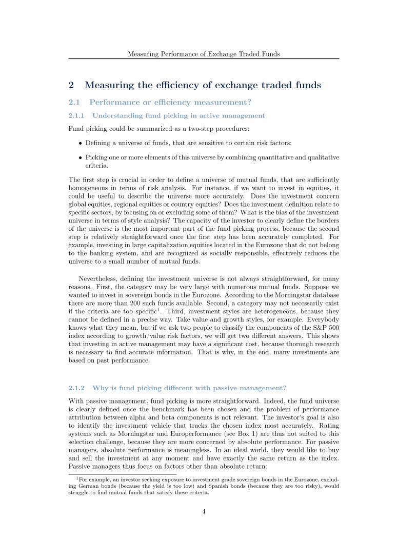
We gave an example of the tracking-error efficient frontier in Figure 3. It is a straight linewhen there is no restriction (Roll, 1992). If we impose some constraints, the efficient frontieris moved to the left and is no longer a straight line.

To compare the performance of different portfolios, a better measure than the Sharperatio is the information ratio, which is defined as follows (Grinold and Kahn, 2000):

IR (x | b) =µ (x | b)σ (x | b)

=(x− b)

⊤µ√

(x− b)⊤Σ(x− b)

If we consider a combination of the benchmark b and the active portfolio x, the compositionof the portfolio is:

y = (1− α) b+ αx

with α ≥ 0 the proportion of wealth invested in the portfolio x. We get:

µ (y | b) = (y − b)⊤µ = αµ (x | b)

and:σ2 (y | b) = (y − b)

⊤Σ(y − b) = α2σ2 (x | b)

We deduce that:µ (y | b) = IR (x | b) · σ (y | b)

It is the equation of a linear function between the expected tracking error and the trackingerror volatility of the portfolio y. It implies that the efficient frontier is a straight line:

4In IOSCO terminology, µ (x | b) corresponds to Tracking Difference (TD) whereas σ (x | b) is calledTracking Error (TE).

7


Figure 3: Tracking-error efficient frontier

“If the manager is measured solely in terms of excess-return performance, he orshe should pick a point on the upper part of this efficient frontier. For instance,the manager may have a utility function that balances expected value addedagainst tracking-error volatility. Note that because the efficient set consists ofa straight line, the maximal Sharpe ratio is not a usable criterion for portfolioallocation” (Jorion, 2003, page 172).

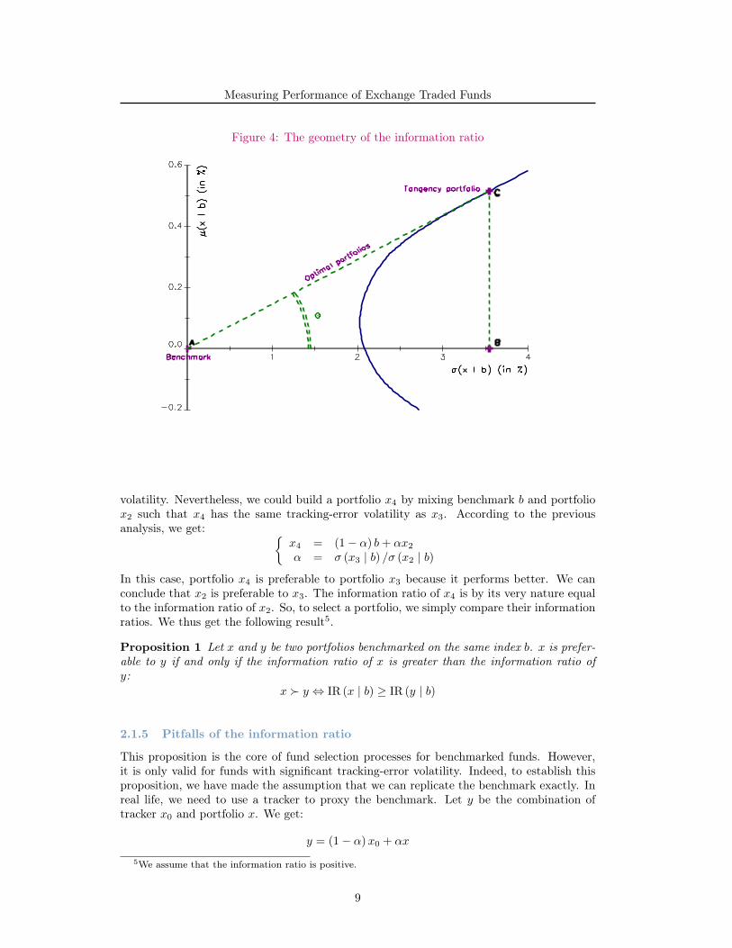
If we add some other constraints to the portfolio optimization problem, the efficient frontieris no more a straight line. In this case, one optimized portfolio dominates all the otherportfolios. It is the portfolio that belongs to the efficient frontier and the straight line thatis tangent to the efficient frontier. It is also the portfolio that maximizes the informationratio. An illustration is provided in Figure 4. In this case, we check that the tangencyportfolio is the one that maximizes the tangent θ, which is the information ratio:

tan θ =BC

AB

=µ (x | b)σ (x | b)

= IR (x | b)

2.1.4 The information ratio as a selection criteria for benchmarked funds

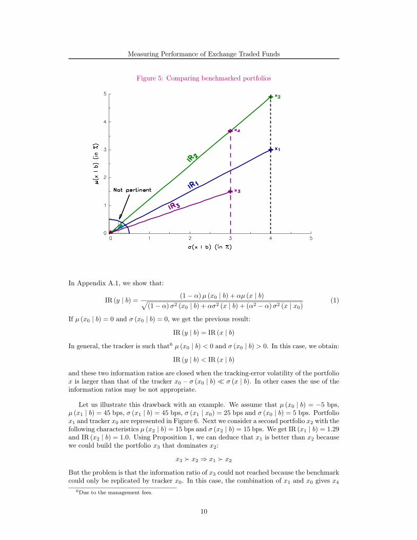
To understand why the information ratio is suitable for comparing benchmarked funds, weconsider the example given in Figure 5. It is obvious that portfolio x2 is preferable toportfolio x1 because it has a better excess-return performance for the same tracking-errorvolatility. If we compare portfolios x3 and x2, they don’t have the same tracking-error

8


Figure 4: The geometry of the information ratio

volatility. Nevertheless, we could build a portfolio x4 by mixing benchmark b and portfoliox2 such that x4 has the same tracking-error volatility as x3. According to the previousanalysis, we get:

x4 = (1− α) b+ αx2

α = σ (x3 | b) /σ (x2 | b)

In this case, portfolio x4 is preferable to portfolio x3 because it performs better. We canconclude that x2 is preferable to x3. The information ratio of x4 is by its very nature equalto the information ratio of x2. So, to select a portfolio, we simply compare their informationratios. We thus get the following result5.

Proposition 1 Let x and y be two portfolios benchmarked on the same index b. x is prefer-able to y if and only if the information ratio of x is greater than the information ratio ofy:

x ≻ y ⇔ IR (x | b) ≥ IR (y | b)

2.1.5 Pitfalls of the information ratio

This proposition is the core of fund selection processes for benchmarked funds. However,it is only valid for funds with significant tracking-error volatility. Indeed, to establish thisproposition, we have made the assumption that we can replicate the benchmark exactly. Inreal life, we need to use a tracker to proxy the benchmark. Let y be the combination oftracker x0 and portfolio x. We get:

y = (1− α)x0 + αx

5We assume that the information ratio is positive.

9


Figure 5: Comparing benchmarked portfolios

In Appendix A.1, we show that:

IR (y | b) = (1− α)µ (x0 | b) + αµ (x | b)√(1− α)σ2 (x0 | b) + ασ2 (x | b) + (α2 − α)σ2 (x | x0)

(1)

If µ (x0 | b) = 0 and σ (x0 | b) = 0, we get the previous result:

IR (y | b) = IR (x | b)

In general, the tracker is such that6 µ (x0 | b) < 0 and σ (x0 | b) > 0. In this case, we obtain:

IR (y | b) < IR (x | b)

and these two information ratios are closed when the tracking-error volatility of the portfoliox is larger than that of the tracker x0 – σ (x0 | b) ≪ σ (x | b). In other cases the use of theinformation ratios may be not appropriate.

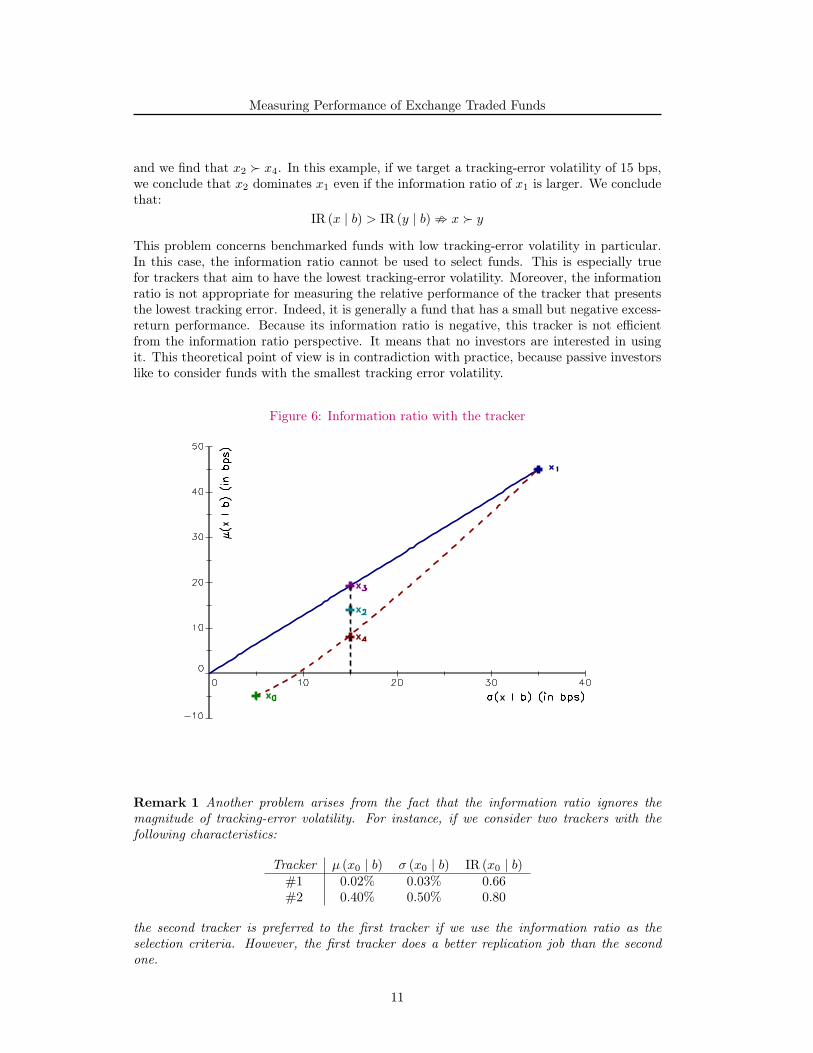
Let us illustrate this drawback with an example. We assume that µ (x0 | b) = −5 bps,µ (x1 | b) = 45 bps, σ (x1 | b) = 45 bps, σ (x1 | x0) = 25 bps and σ (x0 | b) = 5 bps. Portfoliox1 and tracker x0 are represented in Figure 6. Next we consider a second portfolio x2 with thefollowing characteristics µ (x2 | b) = 15 bps and σ (x2 | b) = 15 bps. We get IR (x1 | b) = 1.29and IR (x2 | b) = 1.0. Using Proposition 1, we can deduce that x1 is better than x2 becausewe could build the portfolio x3 that dominates x2:

x3 ≻ x2 ⇒ x1 ≻ x2

But the problem is that the information ratio of x3 could not reached because the benchmarkcould only be replicated by tracker x0. In this case, the combination of x1 and x0 gives x4

6Due to the management fees.

10


and we find that x2 ≻ x4. In this example, if we target a tracking-error volatility of 15 bps,we conclude that x2 dominates x1 even if the information ratio of x1 is larger. We concludethat:

IR (x | b) > IR (y | b) ; x ≻ y

This problem concerns benchmarked funds with low tracking-error volatility in particular.In this case, the information ratio cannot be used to select funds. This is especially truefor trackers that aim to have the lowest tracking-error volatility. Moreover, the informationratio is not appropriate for measuring the relative performance of the tracker that presentsthe lowest tracking error. Indeed, it is generally a fund that has a small but negative excess-return performance. Because its information ratio is negative, this tracker is not efficientfrom the information ratio perspective. It means that no investors are interested in usingit. This theoretical point of view is in contradiction with practice, because passive investorslike to consider funds with the smallest tracking error volatility.

Figure 6: Information ratio with the tracker

Remark 1 Another problem arises from the fact that the information ratio ignores themagnitude of tracking-error volatility. For instance, if we consider two trackers with thefollowing characteristics:

Tracker µ (x0 | b) σ (x0 | b) IR (x0 | b)#1 0.02% 0.03% 0.66#2 0.40% 0.50% 0.80

the second tracker is preferred to the first tracker if we use the information ratio as theselection criteria. However, the first tracker does a better replication job than the secondone.

11


2.2 A comprehensive efficiency indicator for trackersLet us consider a simple model with two periods. The investor buy the tracker x at timet = 0 and sells it at time t = 1. Note the corresponding tracking error e. The relative PnLof the investor with respect to the benchmark b is:

Π(x | b) = e− s (x | b)

where s (x | b) is the bid-ask spread of the tracker. We define the loss L (x | b) of the investoras follows:

L (x | b) = −Π(x | b)The tracker efficiency measure is a risk measure applied to the loss function L (x | b) of theinvestor. We propose to use value-at-risk, which is today commonly accepted as a standardrisk measure. In this case, the efficiency measure ζα (x | b) is defined as follows7:

ζα (x | b) = −inf ζ : Pr L (x | b) ≤ ζ ≥ α

This means that the investor has a probability of 1 − α of losing an amount greater than−ζα (x | b). Let F be the probability distribution function of L (x | b). We get:

ζα (x | b) = −F−1 (α)

If we consider the tracking error model of the previous section and if we assume that assetreturns are Gaussian, we obtain the closed-form formula shown in Appendix A.2. We canthen derive the following definition:

Definition 1 The efficiency measure ζα (x | b) of the tracker x with respect to the benchmarkb corresponds to:

ζα (x | b) = µ (x | b)− s (x | b)− Φ−1 (α)σ (x | b) (2)

where µ (x | b) is the expected value of the tracking error, s (x | b) is the bid-ask spread andσ (x | b) is the volatility of the tracking error.

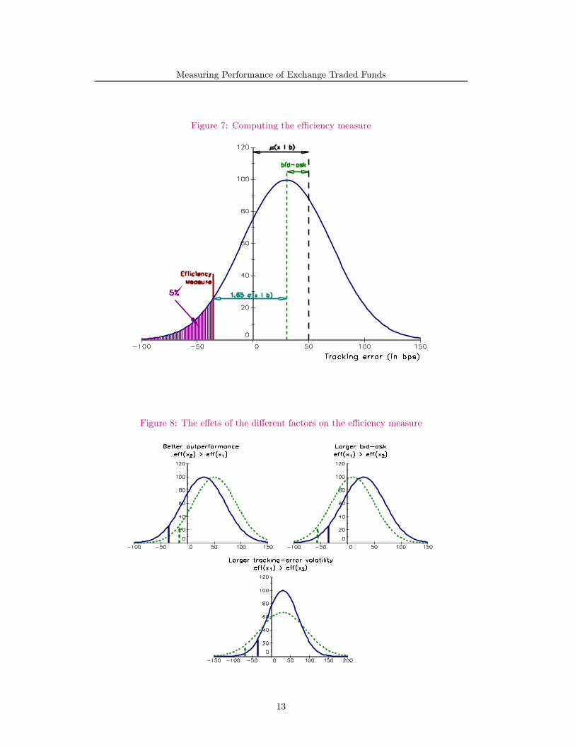
We illustrate the computation of the efficiency measure in Figure 7 when the confidencelevel α is set to 95%. We assume that µ (x | b) = 50 bps, σ (x | b) = 40 bps and s (x | b) = 20bps. The curve corresponds to the density function of the PnL of the investor. It is notcentered on µ (x | b) because of the cost of selling the tracker. It explains that the mean ofthe P&L is 30 bps. According to the Gaussian hypothesis, there is a 50% probability thatthe investor’s gain is greater than 30 bps, but there is also a 50% probability that investor’sgain will be less than 30 bps. The probability of the investor making a loss is therefore equalto 22.66%. To compute the efficiency measure of the tracker, we take the quantile at 5%.We finally obtain ζα (x | b) = −35.79 bps.

In Figure 8, we show the impact of the different factors on the efficiency measure. Thesolid line corresponds to the previous parameter values whereby we modify one parametervalue for each dashed line. For instance, in the first panel, we consider that µ (x | b) isequal to 70 bps. This tracker is preferred as the original tracker because it has a betterexcess-return performance, the same tracking error volatility and the same bid-ask spread.In the second panel, the second tracker has a wider spread8. In this case, we prefer thefirst tracker. For the third panel, we obtain the same conclusion if the second tracker has agreater tracking error volatility. We can then deduce the following result:

7We consider the opposite of the loss in order to obtain an ascending order: the bigger the efficiencymeasure, the better the tracker.

8It is equal to 40 bps.

12


Figure 7: Computing the efficiency measure

Figure 8: The effets of the different factors on the efficiency measure

13


Proposition 2 Let x and y be two trackers benchmarked to the same index b. x is preferableto y if and only if the efficiency measure of x is larger than the efficiency measure of y:

x ≻ y ⇔ ζα (x | b) ≥ ζα (y | b)

Example 1 We consider two trackers x and y with the following characteristics: µ (x | b) =40 bps, s (x | b) = 20 bps, σ (x | b) = 30 bps, µ (x | b) = 30 bps, s (x | b) = 15 bps, σ (x | b) =20 bps. We have Φ−1 (α) = 1.65 at the confidence level 95%. It follows that:

ζα (x | b) = 40− 20− 1.65× 30

= −29.5

and:

ζα (y | b) = 30− 15− 1.65× 20

= −18.0

Because ζα (y | b) > ζα (x | b), we can deduce that tracker y is more efficient than tracker x.A loss of more than 29.5 bps has a 5% probability of occurring for tracker x. In the case oftracker y, this loss is only 18 bps for the same level of probability.

3 Empirical resultsIn this paragraph, we apply the efficiency measure ζα (x | b) to the European ETF market.The confidence level is set at 95%. Let [t0, T ] be the study period with n trading dates. Wecompute ζα (x | b) as follows:

ζα (x | b) = µ (x | b)− s (x | b)− 1.65 · σ (x | b)

where µ (x | b), s (x | b) and σ (x | b) are the estimated statistics for the given study period.We have:

µ (x | b) =

(VT (x)

Vt0 (x)

)1/(T−t0)

−(VT (b)

Vt0 (b)

)1/(T−t0)

s (x | b) =1

n

T∑t=t0

st (x | b)

µ (x | b) =1

n− 1

T∑t=t0+1

Rt (x)−1

n− 1

T∑t=t0+1

Rt (b)

σ (x | b) =

√√√√ 260

n− 1

T∑t=t0+1

(Rt (x)−Rt (b)− µ (x | b))2

where Vt (x) (or Vt (b)) is the net asset value of the tracker (or benchmark) at time t, st (x | b)is the bid-ask spread9 at time t and Rt (x) (or Rt (b)) is the daily return of the tracker (orthe benchmark) defined as follows:

Rt (x) =Vt (x)

Vt−1 (x)− 1

9More precisely, we compute the best spread of the first limit order for each listing place and each tradingday t. st (x | b) is then the weighted average by considering the daily volume of the different listing places.

14


3.1 An application to European ETFsThe study period begins in November, 30th 2011 and ends in November, 30th 2012. Weconsider three benchmarks: the Eurostoxx 50 index, the S&P 500 index and the MSCIWorld index. To compute the statistic ζα (x | b) properly, we need to make some statisticaladjustments:

• Some ETFs distribute dividends. In this case, we have to rebuild the net asset value byincorporating these dividends in order to compute performance that can be comparedto the performance of the benchmark.

• Dividends also influence the tracking-error volatility. That is why we correct the dailyperformance of the tracker every time a dividend is paid.

• Some ETFs have poor liquidity meaning, that we cannot observe a spread for eachtrading date. To compute s (x | b), we decide to exclude dates with zero tradingvolume.

• ETFs may be listed in different currencies. We therefore adopt the point of view of aEuropean investor and consider the Euro as the default currency.

Table 1: Computation of the efficiency measure (Eurostoxx 50)

Tracker µ (x) µ (x | b) s (x | b) σ (x) σ (x | b) ζα (x | b)Amundi 15.29 62.56 9.84 22.33 11.97 32.98db X-trackers 15.33 65.97 12.27 22.86 7.31 41.64iShares (DE) 15.05 37.88 7.96 21.62 56.54 −63.38iShares 15.25 58.46 10.39 21.92 19.62 15.70Lyxor 15.30 63.51 8.48 22.01 14.89 30.47Source 14.90 23.51 15.38 22.23 7.25 −3.83Index 14.67 22.09

Table 2: Computation of the efficiency measure (S&P 500)

Tracker µ (x) µ (x | b) s (x | b) σ (x) σ (x | b) ζα (x | b)Amundi 19.49 9.19 16.97 12.59 3.14 −12.97Credit Suisse 19.57 16.99 18.23 12.50 4.63 −8.88db X-trackers 19.56 16.04 18.26 12.79 4.65 −9.90HSBC 19.68 28.20 20.58 12.68 3.45 1.92iShares 19.34 −6.10 7.45 12.56 4.90 −21.63Lyxor 19.60 19.87 13.56 12.59 0.98 4.69Source 19.34 −5.30 17.81 12.87 1.78 −26.04UBS 19.40 0.02 41.13 12.85 0.59 −42.09Index 19.40 12.76

Results10 are reported in Tables 1, 2 and 3. According to the efficiency measure ζα (x | b),the best tracker for the Eurostoxx 50 index is db X-trackers, followed by Amundi and Lyxor.We notice that ζα (x | b) assigns a positive value to most of the trackers, due probably to

10All the statistics are expressed in bps except µ (x) and σ (x) which are measured in %.

15


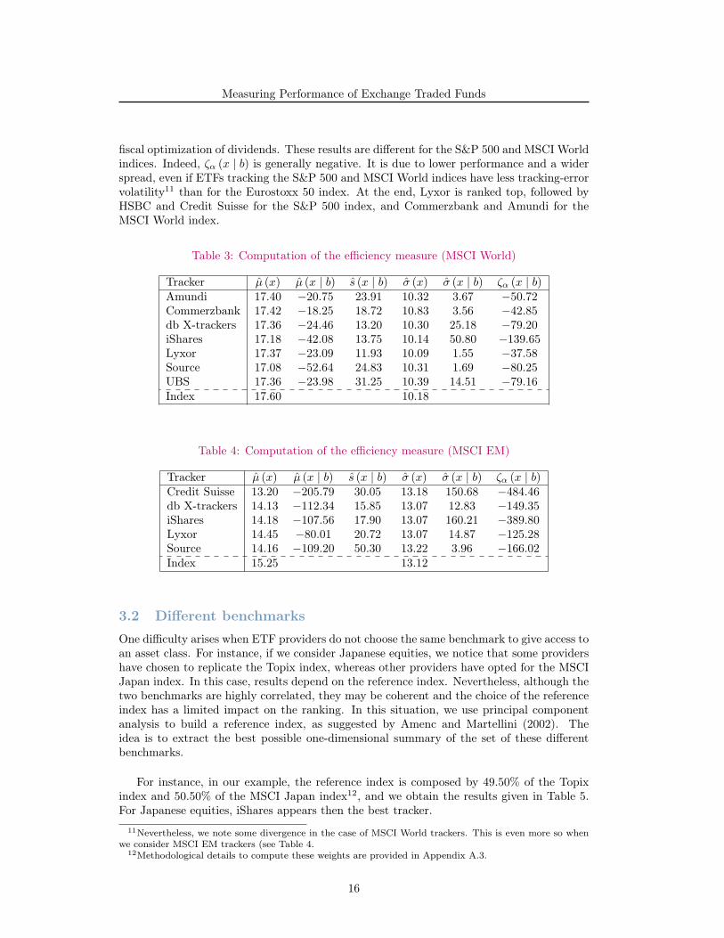
fiscal optimization of dividends. These results are different for the S&P 500 and MSCI Worldindices. Indeed, ζα (x | b) is generally negative. It is due to lower performance and a widerspread, even if ETFs tracking the S&P 500 and MSCI World indices have less tracking-errorvolatility11 than for the Eurostoxx 50 index. At the end, Lyxor is ranked top, followed byHSBC and Credit Suisse for the S&P 500 index, and Commerzbank and Amundi for theMSCI World index.

Table 3: Computation of the efficiency measure (MSCI World)

Tracker µ (x) µ (x | b) s (x | b) σ (x) σ (x | b) ζα (x | b)Amundi 17.40 −20.75 23.91 10.32 3.67 −50.72Commerzbank 17.42 −18.25 18.72 10.83 3.56 −42.85db X-trackers 17.36 −24.46 13.20 10.30 25.18 −79.20iShares 17.18 −42.08 13.75 10.14 50.80 −139.65Lyxor 17.37 −23.09 11.93 10.09 1.55 −37.58Source 17.08 −52.64 24.83 10.31 1.69 −80.25UBS 17.36 −23.98 31.25 10.39 14.51 −79.16Index 17.60 10.18

Table 4: Computation of the efficiency measure (MSCI EM)

Tracker µ (x) µ (x | b) s (x | b) σ (x) σ (x | b) ζα (x | b)Credit Suisse 13.20 −205.79 30.05 13.18 150.68 −484.46db X-trackers 14.13 −112.34 15.85 13.07 12.83 −149.35iShares 14.18 −107.56 17.90 13.07 160.21 −389.80Lyxor 14.45 −80.01 20.72 13.07 14.87 −125.28Source 14.16 −109.20 50.30 13.22 3.96 −166.02Index 15.25 13.12

3.2 Different benchmarks

One difficulty arises when ETF providers do not choose the same benchmark to give access toan asset class. For instance, if we consider Japanese equities, we notice that some providershave chosen to replicate the Topix index, whereas other providers have opted for the MSCIJapan index. In this case, results depend on the reference index. Nevertheless, although thetwo benchmarks are highly correlated, they may be coherent and the choice of the referenceindex has a limited impact on the ranking. In this situation, we use principal componentanalysis to build a reference index, as suggested by Amenc and Martellini (2002). Theidea is to extract the best possible one-dimensional summary of the set of these differentbenchmarks.

For instance, in our example, the reference index is composed by 49.50% of the Topixindex and 50.50% of the MSCI Japan index12, and we obtain the results given in Table 5.For Japanese equities, iShares appears then the best tracker.

11Nevertheless, we note some divergence in the case of MSCI World trackers. This is even more so whenwe consider MSCI EM trackers (see Table 4.

12Methodological details to compute these weights are provided in Appendix A.3.

16


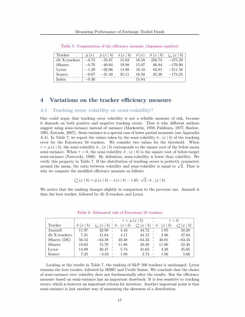
Table 5: Computation of the efficiency measure (Japanese equities)

Tracker µ (x) µ (x | b) s (x | b) σ (x) σ (x | b) ζα (x | b)db X-trackers −0.72 −35.87 15.82 16.58 256.73 −475.29iShares −0.76 −40.64 19.98 15.97 66.84 −170.90Lyxor −1.29 −92.96 14.98 16.10 62.81 −211.58Source −0.67 −31.40 35.11 16.58 65.30 −174.25Index −0.36 15.84

4 Variations on the tracker efficiency measure

4.1 Tracking error volatility or semi-volatility?

One could argue that tracking error volatility is not a reliable measure of risk, becauseit depends on both positive and negative tracking errors. That is why different authorssuggest using semi-variance instead of variance (Markowitz, 1959; Fishburn, 1977; Harlow,1991; Estrada, 2007). Semi-variance is a special case of lower partial moments (see AppendixA.4). In Table 7, we report the values taken by the semi-volatility σ− (x | b) of the trackingerror for the Eurostoxx 50 trackers. We consider two values for the threshold. Whenτ = µ (x | b), the semi-volatility σ− (x | b) corresponds to the square root of the below-meansemi-variance. When τ = 0, the semi-volatility σ− (x | b) is the square root of below-targetsemi-variance (Nawrocki, 1999). By definition, semi-volatility is lower than volatility. Weverify this property in Table 7. If the distribution of tracking errors is perfectly symmetricaround the mean, the ratio between volatility and semi-volatility is equal to

√2. That is

why we compute the modified efficiency measure as follows:

ζ⋆α (x | b) = µ (x | b)− s (x | b)− 1.65 ·√2 · σ− (x | b)

We notice that the ranking changes slightly in comparison to the previous one. Amundi isthus the best tracker, followed by db X-trackers and Lyxor.

Table 6: Estimated risk of Eurostoxx 50 trackers

τ = µ (x | b) τ = 0Tracker σ (x | b) ζα (x | b) σ− (x | b) ζ⋆α (x | b) σ− (x | b) ζ⋆α (x | b)Amundi 11.97 32.98 3.43 44.72 1.05 50.28db X-trackers 7.31 41.64 4.11 44.12 2.86 47.04iShares (DE) 56.54 −63.38 40.38 −64.32 40.01 −63.45iShares 19.62 15.70 11.86 20.38 11.00 22.40Lyxor 14.89 30.47 5.74 41.63 4.28 45.05Source 7.25 −3.83 1.88 3.74 1.06 5.66

Looking at the results in Table 7, the ranking of S&P 500 trackers is unchanged: Lyxorremains the best tracker, followed by HSBC and Credit Suisse. We conclude that the choiceof semi-variance over volatility does not fundamentally alter the results. But the efficiencymeasure based on semi-variance has an important drawback. It is less sensitive to trackingerrors, which is however an important criteria for investors. Another important point is thatsemi-variance is just another way of measuring the skewness of a distribution:

17


Table 7: Estimated risk of S&P 500 trackers

τ = µ (x | b) τ = 0Tracker σ (x | b) ζα (x | b) σ− (x | b) ζ⋆α (x | b) σ− (x | b) ζ⋆α (x | b)Amundi 3.14 −12.97 1.22 −10.64 0.84 −9.74Credit Suisse 4.63 −8.88 3.01 −8.26 2.53 −7.13db X-trackers 4.65 −9.90 3.39 −10.13 2.91 −9.01HSBC 3.45 1.92 2.01 2.92 1.25 4.71iShares 4.90 −21.63 3.26 −21.15 3.34 −21.34Lyxor 0.98 4.69 0.68 4.73 0.28 5.67Source 1.78 −26.04 1.10 −25.67 1.23 −25.97UBS 0.59 −42.09 0.37 −41.98 0.35 −41.93

“By taking the variance and dividing it by the below-mean semi-variance, ameasure of skewness resulted. If the distribution is normally distributed thenthe semi-variance should be one-half of the variance [...] If the ratio is notequal to 2, then there is evidence that the distribution is skewed or asymmetric”(Nawrocki, 1999, page 11).

If we compute this ratio for the previous trackers, we get a range between 1.9 and 14.8for the Eurostoxx 50 index and between 1.9 and 6.6 for the S&P 500 index. This clearlydemonstrates that tracking errors exhibit high skewness. This result is confirmed by theKernel analysis of empirical density (see Figures 9, 10 and 11). In this context, we thinkthat replacing volatility by semi-volatility is not a good method. It would be better to adoptanother risk measure that takes the skewness of tracking errors into account.

Figure 9: Estimated density of daily tracking errors (Eurostoxx 50)

18


Figure 10: Estimated density of daily tracking errors (S&P 500)

Figure 11: Estimated density of daily tracking errors (S&P 500)

19


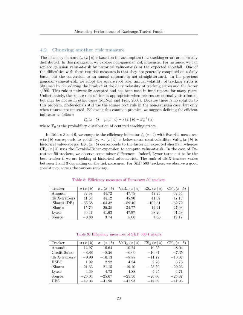
4.2 Choosing another risk measureThe efficiency measure ζα (x | b) is based on the assumption that tracking errors are normallydistributed. In this paragraph, we explore non-gaussian risk measures. For instance, we canreplace gaussian value-at-risk by historical value-at-risk or the expected shortfall. One ofthe difficulties with these two risk measures is that they are generally computed on a dailybasis, but the conversion to an annual measure is not straightforward. In the previousgaussian value-at-risk, we adopt the square root rule: annual volatility of tracking errors isobtained by considering the product of the daily volatility of tracking errors and the factor√260. This rule is universally accepted and has been used in fund reports for many years.

Unfortunately, the square root of time is appropriate when returns are normally distributed,but may be not so in other cases (McNeil and Frey, 2000). Because there is no solution tothis problem, professionals still use the square root rule in the non-gaussian case, but onlywhen returns are centered. Following this common practice, we suggest defining the efficientindicator as follows:

ζ⋆α (x | b) = µ (x | b)− s (x | b)− F−10 (α)

where F0 is the probability distribution of centered tracking errors.

In Tables 8 and 9, we compute the efficiency indicator ζα (x | b) with five risk measures:σ (x | b) corresponds to volatility, σ− (x | b) is below-mean semi-volatility, VaRα (x | b) ishistorical value-at-risk, ESα (x | b) corresponds to the historical expected shortfall, whereasCFα (x | b) uses the Cornish-Fisher expansion to compute value-at-risk. In the case of Eu-rostoxx 50 trackers, we observe some minor differences. Indeed, Lyxor turns out to be thebest tracker if we are looking at historical value-at-risk. The rank of db X-trackers variesbetween 1 and 3 depending on the risk measures. For S&P 500 trackers, we observe a goodconsistency across the various rankings.

Table 8: Efficiency measures of Eurostoxx 50 trackers

Tracker σ (x | b) σ− (x | b) VaRα (x | b) ESα (x | b) CFα (x | b)Amundi 32.98 44.72 47.75 47.25 62.54db X-trackers 41.64 44.12 45.90 41.02 47.15iShares (DE) −63.38 −64.32 −59.40 −102.51 −62.72iShares 15.70 20.38 34.77 12.21 27.93Lyxor 30.47 41.63 47.97 38.26 61.48Source −3.83 3.74 5.00 4.63 19.17

Table 9: Efficiency measures of S&P 500 trackers

Tracker σ (x | b) σ− (x | b) VaRα (x | b) ESα (x | b) CFα (x | b)Amundi −12.97 −10.64 −10.24 −10.55 −8.04Credit Suisse −8.88 −8.26 −6.60 −10.37 −7.35db X-trackers −9.90 −10.13 −8.88 −11.77 −10.02HSBC 1.92 2.92 4.24 2.23 3.73iShares −21.63 −21.15 −19.10 −23.59 −20.23Lyxor 4.69 4.73 4.88 4.25 4.71Source −26.04 −25.67 −25.50 −26.00 −25.37UBS −42.09 −41.98 −41.93 −42.09 −41.95

20


4.3 Taking the liquidity risk into accountThe spread measure s (x | b) used previously corresponds to the daily average of the firstlimit order spreads. This measure may be pertinent for a retail investor, but is not for aninstitutional investor. Institutional investors buy or sell a notional N , that can not generallybe executed via the best first limit orders. That is why we consider another spread measuresN (x | b) corresponding to intraday spreads weighted by the duration between two ticks fora given notional13. To illustrate the use of this spread, we are going to look at the Eurostoxx50 trackers.

Figure 12: Evolution of the spread of the Amundi tracker

In Figure 12, we shown the change in the spread sN (x | b) for the Amundi Eurostoxx50 tracker and different values of the notional N . We notice that this spread changes withrespect to market liquidity. For each tracker and each notional value, we have shown thecorresponding boxplot in Figure 13. The boxplot indicates the minimum value, the quartilerange, the median and the last decile. We check that:

N1 ≥ N2 ⇒ sN1 (x | b) ≥ sN2 (x | b)

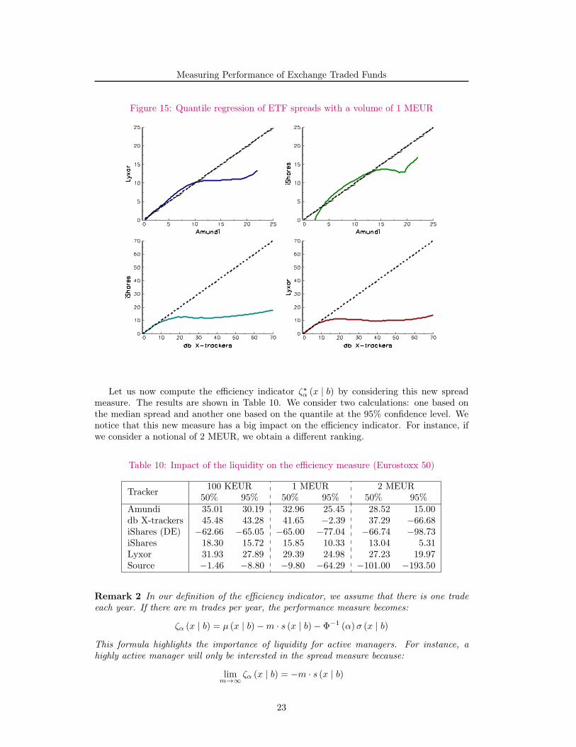
We notice also that for some trackers, the spread increases greatly in line with volume.In Figure 14, we have drawn some scatterplots. It is interesting to note that when liquidityis not an issue, the trackers are more or less equivalent in terms of spread14. This is not thecase when there are some liquidity problems (see Figure 15).

13Computational details are provided in Appendix A.5.14If we consider two trackers x and y, we have:

sN (x | b) ≃ sN (y | b)

if sN (x | b) ≃ 0 and sN (x | b) ≃ 0.

21


Figure 13: Boxplot of ETF spreads

Figure 14: Scatterplot of ETF spreads with a volume of 1 MEUR

22


Figure 15: Quantile regression of ETF spreads with a volume of 1 MEUR

Let us now compute the efficiency indicator ζ⋆α (x | b) by considering this new spreadmeasure. The results are shown in Table 10. We consider two calculations: one based onthe median spread and another one based on the quantile at the 95% confidence level. Wenotice that this new measure has a big impact on the efficiency indicator. For instance, ifwe consider a notional of 2 MEUR, we obtain a different ranking.

Table 10: Impact of the liquidity on the efficiency measure (Eurostoxx 50)

Tracker 100 KEUR 1 MEUR 2 MEUR50% 95% 50% 95% 50% 95%

Amundi 35.01 30.19 32.96 25.45 28.52 15.00db X-trackers 45.48 43.28 41.65 −2.39 37.29 −66.68iShares (DE) −62.66 −65.05 −65.00 −77.04 −66.74 −98.73iShares 18.30 15.72 15.85 10.33 13.04 5.31Lyxor 31.93 27.89 29.39 24.98 27.23 19.97Source −1.46 −8.80 −9.80 −64.29 −101.00 −193.50

Remark 2 In our definition of the efficiency indicator, we assume that there is one tradeeach year. If there are m trades per year, the performance measure becomes:

ζα (x | b) = µ (x | b)−m · s (x | b)− Φ−1 (α)σ (x | b)

This formula highlights the importance of liquidity for active managers. For instance, ahighly active manager will only be interested in the spread measure because:

limm→∞

ζα (x | b) = −m · s (x | b)

23


5 ConclusionIn this paper, we have developed a performance measure to compare passive management,in particular tracker investment vehicles such as exchange traded funds. This measure isvery different from the ones used to assess the performance of active management. It is avalue-at-risk measure based on three parameters: the performance difference between thefund and the index, the volatility of the tracking error and the liquidity spread. This simplemeasure may be easily implemented by investors or rating agencies in relation to the fundpicking process.

This paper also highlights the role of liquidity spread in measuring the efficiency of anETF. It is particular true for institutional investors, who may subscribe or redeem largeinvestment amounts. The liquidity spread is also the most important parameter for activemanagers who use ETFs to implement their convictions in line with their tactical assetallocation.

24


References

[1] Amenc N. and Martellini L. (2002), The Brave New World of Hedge Fund Indices,EDHEC-Risk Working paper.

[2] Barras L., Scaillet O. and Wermers R. (2010), False Discoveries in Mutual FundPerformance: Measuring Luck in Estimated Alphas, Journal of Finance, 65(1), pp.179-216.

[3] Bawa V.S. (1975), Optimal Rules for Ordering Uncertain Prospects, Journal of Finan-cial Economics, 2(1), pp. 95-121.

[4] Beasley J.E., Meade N. and Chang T.-J. (2003), An Evolutionary Heuristic forthe Index Tracking Problem, European Journal of Operational Research, 148(3), pp.621-643.

[5] Blake C.R., Elton E.J. and Gruber M.J. (1993), The Performance of Bond MutualFunds, Journal of Business, 66(3), pp. 371-403.

[6] Bernstein P.L. (1992), Capital Ideas: The Improbable Origins of Modern Wall Street,Free Press.

[7] Bernstein P.L. (2007), Capital Ideas Evolving, John Wiley & Sons.

[8] Carhart M.M. (1997), On Persistence in Mutual Fund Performance, Journal of Fi-nance, 52(1), pp. 57-82.

[9] Dieterlen R. and Hereil P. (2012), Index Arbitrage Explained, Journal of IndexesEurope, 2(6), pp. 18-23.

[10] Elton E.J., Gruber M.J., Das S. and Hlavka M. (1993), Efficiency with CostlyInformation: A Reinterpretation of Evidence from Managed Portfolios, Review of Fi-nancial Studies, 6(1), pp. 1-22.

[11] Elton E.J., Gruber M.J. and Busse J.A. (2004), Are Investors Rational? Choicesamong Index Funds, Journal of Finance, 59(1), pp. 261-288.

[12] Estrada J. (2007), Mean-semivariance Behavior: Downside Risk and Capital AssetPricing, International Review of Economics and Finance, 16(2), pp. 169-185.

[13] Fishburn P.C. (1977), Mean-Risk Analysis with Risk Associated with Below-TargetReturns, American Economic Review, 67(1), pp. 116-126.

[14] Gastineau G.L. (2002), Equity Index Funds Have Lost Their Way, Journal of PortfolioManagement, 28(2), pp. 55-64.

[15] Gastineau G.L. (2004), The Benchmark Index ETF Performance Problem, Journalof Portfolio Management, 30(2), pp. 96-103.

[16] Grinblatt M. and Titman S. (1989), Portfolio Performance Evaluation: Old Issuesand New Insights, Review of Financial Studies, 2(3), pp. 393-421.

[17] Grinold R.C. and Kahn R.N. (2000), Active Portfolio Management: A Quantita-tive Approach for Providing Superior Returns and Controlling Risk, Second edition,McGraw-Hill.

25


[18] Harlow W.V. (1991), Asset Allocation in a Downside-Risk Framework, FinancialAnalysts Journal, 47(5), pp. 28-40.

[19] Jensen M.C. (1968), The Performance of Mutual Funds in the Period 1945-1964, Jour-nal of Finance, 23(2), pp. 389-416.

[20] Jorion P. (2003), Portfolio Optimization with Tracking-Error Constraints, FinancialAnalysts Journal, 59(5), pp. 70-82.

[21] Markowitz H. (1952), Portfolio Selection, Journal of Finance, 7(1), pp. 77-91.

[22] Markowitz H. (1959), Portfolio Selection: Efficient Diversification of Investments,John Wiley & Sons.

[23] McNeil A.J. and Frey R. (2000), Estimation of Tail-related Risk Measures for Het-eroscedastic Financial Time Series: An Extreme Value Approach, Journal of EmpiricalFinance, 7(3-4), pp. 271-300.

[24] Nawrocki D.N. (1999), A Brief History of Downside Risk Measures, Journal of In-vesting, 8(3), pp. 9-25.

[25] Pope P.F. and Yadav P.K. (1994), Discovering Errors in Tracking Error, Journal ofPortfolio Management, 20(2), pp. 27-32.

[26] Prigent J.-L. (2007), Portfolio Optimization and Performance Analysis, Chapman &Hall.

[27] Roll R. (1992), A Mean/Variance Analysis of Tracking Error, Journal of PortfolioManagement, 18(4), pp. 13-22.

[28] Sharpe W.F. (1964), Capital Asset Prices: A Theory of Market Equilibrium underConditions of Risk, Journal of Finance, 19(3), pp. 425-442.

[29] Tobin J. (1958), Liquidity Preference as Behavior Towards Risk, Review of EconomicStudies, 25(2), pp. 65-86.

26


A.2 Derivation of the efficiency measure ζα (x | b)The probability distribution function of the tracking error e is Gaussian with:

e ∼ N(µ (x | b) , σ2 (x | b)

)We have:

Pr L (x | b) ≤ ζ = α

⇔ Pr e− s ≤ ζ = α

⇔ Pr e ≤ s+ ζ = α

⇔ Pr

e− µ (x | b)σ (x | b)

≤ s+ ζ − µ (x | b)σ (x | b)

= α

⇔ Φ

(s+ ζ − µ (x | b)

σ (x | b)

)= α

It follows that:s+ ζ − µ (x | b)

σ (x | b)= Φ−1 (α)

or:ζ = s− µ (x | b) + Φ−1 (α)σ (x | b)

We deduce that:

ζα (x | b) = −ζ

= µ (x | b)− s− Φ−1 (α)σ (x | b)

A.3 Building a benchmark from a set of competing indicesLet b1, . . . , bm be a set of competing indices. The underlying idea is to compute a bench-mark b representative of these indices. Let Ω be the m×m covariance matrix of the returnsRt (bj). By computing the eigendecomposition of Ω, we get:

Ω = V ΛV ⊤ (3)

where V is the matrix of the eigenvectors and Λ = diag (λ1, . . . , λm) is a diagonal matrixof eigenvalues15. Because the decomposition (3) corresponds to the principal componentanalysis (PCA), we may extract the main representative factor defined by:

Ft =

m∑j=1

Vj,1Rt (bj)

As noticed by Amenc and Martellini (2002), this first component of the PCA maximizes therepresentativeness of the set of competing indices. The reference index is then a weightedportfolio of the competing indices:

b =m∑j=1

wjbj

where the weights are proportional to the loading coefficients:

wj =Vj,1∑m

k=1 Vk,1

15We assume that λ1 ≥ . . . ≥ λm.

28


A.4 Lower partial moments

Let X be a random variable with distribution F. The mathematical expectation of X is16:

µ = E [X]

=

∫ ∞

−∞xdF (x)

=

∫ ∞

−∞xf (x) dx

whereas the centered moment of order n is:

µn (X) = E [(X − µ)n]

=

∫ ∞

−∞(x− µ)

nf (x) dx

The variance of X corresponds to the second moment: σ2 (X) = µ2 (X). σ (X) is calledstandard deviation, but it is well known as volatility in finance, where X represents thereturn on an asset.

The lower partial moment (LPM) is obtained by (Bawa, 1975):

LPMn (X; τ) = E [max (0, τ −X)n]

=

∫ τ

−∞(τ − x)

nf (x) dx

where τ is a threshold. If τ is equal to the mean µ, we get:

LPMn (X;µ) = E [max (0, µ−X)n]

=

∫ µ

−∞(µ− x)

nf (x) dx

Semi-variance is then defined as the second lower partial moment:

SV (x) = LPM2 (X;µ)

= E[max (0, µ−X)

2]

=

∫ µ

−∞(µ− x)

2f (x) dx

If the distribution of X is symmetric around the mean, we get:∫ ∞

−∞(µ− x)

2f (x) dx =

∫ µ

−∞(µ− x)

2f (x) dx+

∫ ∞

µ

(µ− x)2f (x) dx

= 2

∫ µ

−∞(µ− x)

2f (x) dx

We deduce that semi-variance is half of the variance.

16We note f (x) the associated density function.

29


A.5 Computation of the spread sN (x | b)A.5.1 Analytical expression

We define the daily spread sN (x | b) as a weighted average of intraday spreads:

sN (x | b) =∑close

j=open sj (tj+1 − tj)∑closej=open (tj+1 − tj)

where sj is the spread of the jth tick and tj+1− tj the elapsed time between two consecutiveticks:

sj = cj

(P+j − P−

j

)P 0j

We have also:

P •j =

∑Kk=1 Q

•j,kP

•j,k∑K

k=1 Q•j,k

where P+j,k (resp. P−

j,k) is the ask (or bid) price at tj for the kth limit order. The averagemid price P 0

j corresponds to:

P 0j =

P+j + P−

j

2

The quantity Q+j,k and Q−

j,k are defined as follows:

Q•j,k = max

(0,min

(Q•

j,k, Q⋆j −

k−1∑l=1

Q•j,l

))

Here, Q+j,k and Q−

j,k are the ask and bid volumes of the kth limit order. The referencequantity Q⋆

j is the ratio between the trading notional N and the mid price:

Q⋆j =

N

P 0j

Sometimes it may appear that the trading volume on the order book is lower than thenotional N . That is why the factor cj may be greater than one:

cj = max

1,Q⋆

j

min(∑K

k=1 Q+j,k,∑K

k=1 Q−j,k

)

For instance, if we wish to execute an order of 2 MEUR and there is only a trading volumeof 1 MEUR, we multiply the spread by two.

Remark 3 For each trading day, we compute the daily spread for the different listing placesusing the previous formulas and we take the best spread.

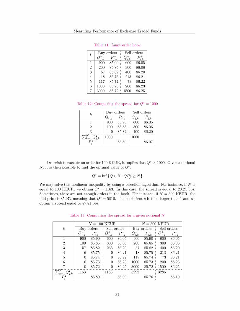
A.5.2 Example

Let us illustrate the spread calculation with the order book given in Table 11. For Q⋆ = 1000,we get the results shown in Table 12. We deduce that the mid price P 0

j is 85.98 whereas thespread sj is equal to 20.12 bps. It corresponds to a notional N = Q⋆ × P 0

j of 85 981 e.

30


Table 11: Limit order book

kBuy orders Sell ordersQ−

j,k P−j,k Q+

j,k P+j,k

1 900 85.90 600 86.052 200 85.85 300 86.063 57 85.82 400 86.204 18 85.75 213 86.215 117 85.74 73 86.226 1000 85.73 200 86.237 3000 85.72 1500 86.25

Table 12: Computing the spread for Q⋆ = 1000

kBuy orders Sell ordersQ−

j,k P−j,k Q+

j,k P+j,k

1 900 85.90 600 86.052 100 85.85 300 86.063 0 85.82 100 86.20∑K

k=1 Q•j,k 1000 1000

P •j 85.89 86.07

If we wish to execute an order for 100 KEUR, it implies that Q⋆ > 1000. Given a notionalN , it is then possible to find the optimal value of Q⋆:

Q⋆ = infQ ∈ N : QP 0

j ≥ N

We may solve this nonlinear inequality by using a bisection algorithm. For instance, if N isequal to 100 KEUR, we obtain Q⋆ = 1163. In this case, the spread is equal to 23.24 bps.Sometimes, there are not enough orders in the book. For instance, if N = 500 KEUR, themid price is 85.972 meaning that Q⋆ = 5816. The coefficient c is then larger than 1 and weobtain a spread equal to 87.81 bps.

Table 13: Computing the spread for a given notional N

kN = 100 KEUR N = 500 KEUR

Buy orders Sell orders Buy orders Sell ordersQ−

j,k P−j,k Q+

j,k P+j,k Q−

j,k P−j,k Q+

j,k P+j,k

1 900 85.90 600 86.05 900 85.90 600 86.052 100 85.85 300 86.06 200 85.85 300 86.063 57 85.82 263 86.20 57 85.82 400 86.204 6 85.75 0 86.21 18 85.75 213 86.215 0 85.74 0 86.22 117 85.74 73 86.216 0 85.73 0 86.23 1000 85.73 200 86.237 0 85.72 0 86.25 3000 85.72 1500 86.25∑K

k=1 Q•j,k 1163 1163 5292 3286

P •j 85.89 86.09 85.76 86.19

31


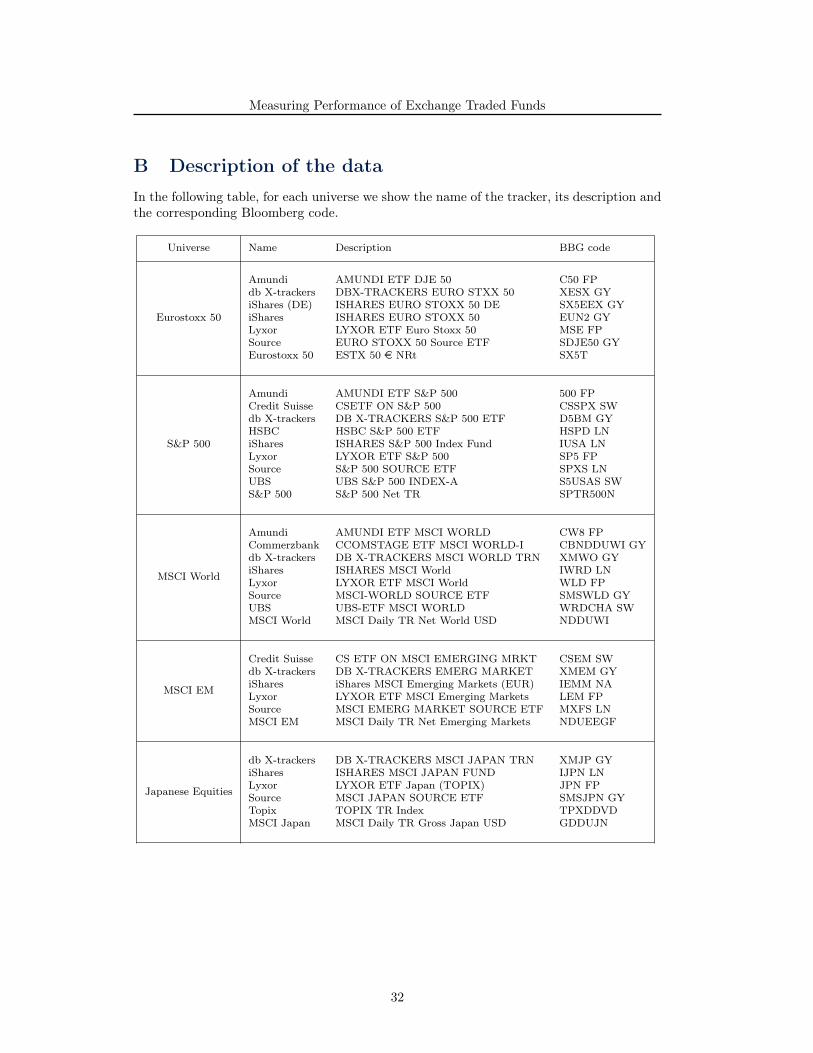
B Description of the dataIn the following table, for each universe we show the name of the tracker, its description andthe corresponding Bloomberg code.

Universe Name Description BBG code

Eurostoxx 50

Amundi AMUNDI ETF DJE 50 C50 FPdb X-trackers DBX-TRACKERS EURO STXX 50 XESX GYiShares (DE) ISHARES EURO STOXX 50 DE SX5EEX GYiShares ISHARES EURO STOXX 50 EUN2 GYLyxor LYXOR ETF Euro Stoxx 50 MSE FPSource EURO STOXX 50 Source ETF SDJE50 GYEurostoxx 50 ESTX 50 e NRt SX5T

S&P 500

Amundi AMUNDI ETF S&P 500 500 FPCredit Suisse CSETF ON S&P 500 CSSPX SWdb X-trackers DB X-TRACKERS S&P 500 ETF D5BM GYHSBC HSBC S&P 500 ETF HSPD LNiShares ISHARES S&P 500 Index Fund IUSA LNLyxor LYXOR ETF S&P 500 SP5 FPSource S&P 500 SOURCE ETF SPXS LNUBS UBS S&P 500 INDEX-A S5USAS SWS&P 500 S&P 500 Net TR SPTR500N

MSCI World

Amundi AMUNDI ETF MSCI WORLD CW8 FPCommerzbank CCOMSTAGE ETF MSCI WORLD-I CBNDDUWI GYdb X-trackers DB X-TRACKERS MSCI WORLD TRN XMWO GYiShares ISHARES MSCI World IWRD LNLyxor LYXOR ETF MSCI World WLD FPSource MSCI-WORLD SOURCE ETF SMSWLD GYUBS UBS-ETF MSCI WORLD WRDCHA SWMSCI World MSCI Daily TR Net World USD NDDUWI

MSCI EM

Credit Suisse CS ETF ON MSCI EMERGING MRKT CSEM SWdb X-trackers DB X-TRACKERS EMERG MARKET XMEM GYiShares iShares MSCI Emerging Markets (EUR) IEMM NALyxor LYXOR ETF MSCI Emerging Markets LEM FPSource MSCI EMERG MARKET SOURCE ETF MXFS LNMSCI EM MSCI Daily TR Net Emerging Markets NDUEEGF

Japanese Equities

db X-trackers DB X-TRACKERS MSCI JAPAN TRN XMJP GYiShares ISHARES MSCI JAPAN FUND IJPN LNLyxor LYXOR ETF Japan (TOPIX) JPN FPSource MSCI JAPAN SOURCE ETF SMSJPN GYTopix TOPIX TR Index TPXDDVDMSCI Japan MSCI Daily TR Gross Japan USD GDDUJN

32

measuring performance of exchange traded funds performance of exchange traded funds 2 measuring the...

Documents