exchange-traded funds and information asymmetry · journal of finance and accountancy...

Journal of Finance and Accountancy

Exchange-traded funds,

Exchange-traded funds and information asymmetry

Dan Zhou California State University at Bakersfield

ABSTRACT

The exchange-traded funds (ETFs) are traded just like shares of common stocks, but they are unit investment trusts and their share prices are directly linked to their respective stock indexes. Theoretical models have predicted that the ETFs markets would attract trading volume from liquidity traders because their losses due to adverse trades with informed traders would usually be lower in ETFs markets than in individual securities markets. This study uses SPDRs and DIAMONDS as examples of ETFs to empirically investigate the hypotheses specified in the theoretical models. Consistent with the hypotheses, we find that the information asymmetry is lower in the ETFs markets than in the market of their underlying individual securities. ETFs markets are more liquid and have lower adverse selection costs and lower trade informativeness compared with their underlying individual securities. Keywords: exchange-traded funds, information asymmetry, liquidity, adverse selection cost, trade informativeness.



1. INTRODUCTION

In the last two decades, one of the most exciting financial innovations is the introduction of exchange-traded funds (ETFs). ETFs are traded just like shares of common stocks, but they are unit investment trusts and their share prices are directly linked to their respective stock

indexes. The first ETF, Standard & Poor’s Depository Receipts (SPDRs) or Spiders, was introduced by the American Stock Exchange (AMEX) on January 29, 1993. It is designed to track the performance of the Standard & Poor’s 500 index. Immediately after the launching, SPDRs have attracted significant trading volume, and have been deemed a great success of product innovation by the AMEX. SPDRs are now one of the most actively traded securities on the New York Stock Exchange (NYSE)1.

The creation of ETFs gives investors an alternative trading vehicle. An investor can choose to buy or sell either the ETFs or the underlying individual securities that compose the indexes. Ackert and Tian (2000) and Elton et al. (2002) examine the characteristics and performance of SPDRs. They show that SPDRs track the S&P 500 index quite precisely.

Given that SPDRs show excellent tracking record, Subrahmanyam (1991), Gorton and Pennacchi (1993) argue that composite securities, such as SPDRs, are not redundant because the return on these securities cannot be replicated by holding the individual underlying stocks when prices are not fully revealing or the market is not completely transparent.

Subrahmanyam (1991) develops a model that characterizes the trading strategy of discretionary uninformed traders. These uninformed traders can choose to trade either in the market for the composite security or in the underlying securities markets. Because of a “diversification” or “information offset” effect of the independent trades of informed traders (who have firm-specific and/or systematic information) in the composite security, the total effect of informed trading is less damaging to the discretionary uninformed traders in the market for the composite security than in the underlying individual securities markets.

Gorton and Pennacchi (1993) concentrate on characterizing the optimal trading strategy of liquidity (uninformed) traders. They illustrate that the composite security can reduce informed traders’ information advantages over uninformed traders. Assuming that investors’ utility function depends only on the mean and variance of return from investing in securities, they show that the presence of a composite security can minimize uninformed traders’ loss to informed traders. The mere operation of informed traders in the markets can reduce uninformed traders’ expected rate of return on any security and increase the return variance, thus reduce their expected utility. Because of the diversification effect, a composite security can always be created to increase the expected utility of the uninformed traders.

Because the introduction of ETFs reduces informed traders’ information advantages, we predict that there is less information asymmetry in the ETFs markets than in the markets for the underlying individual securities. To estimate the information asymmetry, we adopt three proxies: market liquidity, adverse selection cost and trade informativeness. The research indicates market makers usually use the bid-ask spread and depth to manage information asymmetry risk, and market liquidity is a noisy indicator of information asymmetry. Given the relationship between information asymmetry and market liquidity, we predict that ETFs are more liquid, that is, have narrower bid-ask spreads and greater quoted depth.

With lower information asymmetry, the market maker will face less adverse selection risk and narrow the adverse selection component of the bid-ask spread. We thus would predict

1 AMEX was acquired by the NYSE in 2008 and the SPDRs are currently traded on the NYSE.



that ETFs have a lower adverse selection cost than the underlying securities. Researchers find that the extent of information asymmetry is not only positively related to the adverse selection cost, but also positively related to the price impact of the trade. Hasbrouck (1991b) develops two measures of trade informativeness based on the price impact of a trade. We would expect ETFs to have less price impact than trades in the underlying individual securities, i.e., they have a lower extent of trade informativeness than the underlying individual securities.

In this paper, we use the SPDRs and DIAMONDS2 to test the hypothesis of information asymmetry and we find that ETFs are more liquid, i.e., have narrower bid-ask spread and greater quoted depth. Then we use the Glosten and Harris (1988) and Lin, Sanger, and Booth (1995) models to decompose the bid-ask spreads, and find that ETFs have lower adverse selection costs than the underlying individual securities. By using the Hasbrouck (1991a, 1991b) vector autoregressive and vector moving average models, we find that less information is conveyed by trades in the ETFs markets than in the markets for the individual securities, both in absolute and relative terms. 2. METHODOLOGY 2.1. Market Liquidity

Researchers find that market makers usually use the bid-ask spread and depth to manage information asymmetry risk. The relationship between the level of information asymmetry and market liquidity should be negative. That is, higher information asymmetry is associated with wider spreads and less depth and vice versa. The bid-ask spread and depth variables are as follows. Denote At, Bt, and Pt as the ask, bid, and trade prices at time t, and Qt = (At + Bt)/2 as quote midpoint. We examine both bid-ask spread and depth as follows:

• Quoted Dollar Spread = At − Bt.

• Relative Quoted spread = (At − Bt)/ Qt.

• Effective Dollar Spread = 2|Pt − Qt|.

• Effective Relative Spread = 2|log(Pt / Qt)|.

• Depth (number of shares) = Sum of share depth at ask and bid price per quotation.

• Dollar Depth = Sum of dollar depth at ask and bid price per quotation.

• Half-Hour Depth = Sum of all share depth at ask and bid price over the half-hour period.

• Half-Hour Dollar Depth = Sum of all dollar depth at ask and bid price over the half-hour period.

2.2. Adverse selection cost

A large part of the market maker’s profit comes from the bid-ask spread, typically divided into three components: order processing, inventory holding, and adverse selection elements. Because the market makers may trade with unidentified informed traders, they need to widen the bid-ask spread to recover from uninformed traders what they lose to informed traders. We call this the adverse selection component. If market makers face less information asymmetry in a certain market, they should narrow the adverse selection component of the spread in this market.

2 DIAMONDs are designed to track the performance of the Dow Jones Industrial 30 Average.



The adverse selection component of the bid-ask spread is not directly observable, but it has been the subject of extensive study in recent years. To decompose the spread for measuring adverse selection costs, we use Glosten and Harris’s (1988) and Lin, Sanger and Booth’s (1995) models. Van Ness, Van Ness, and Warr (2001) examine the performance of five commonly used spread decomposition models in the finance literature. We conclude that the two models we choose operationally better than others when measuring adverse selection components.

2.2.1. Glosten and Harris (1988) Model

In Glosten and Harris (1988), the bid-ask spread is divided into two components: a transitory component (order processing fee and inventory costs) and a permanent component (adverse selection cost). The transitory component is not related to the underlying value of the securities, which causes the transaction price changes to be negatively serially correlated (Roll, 1984). The permanent component reflects the market maker’s expected value of the security, which does not cause serial correlation in the transaction price changes.

The Glosten and Harris model is represented as follows:

tttt CImP += (1)

ttttt eZImm ++= −1 (2)

tt VccC 10 += (3)

tt VzzZ 10 += (4)

where tP is the transaction price at time t; tm is the unobserved ‘true’ price; tV is the shares

volume traded at time t; tI is a trade indicator that takes a value of +1 if the transaction is buyer-

initiated and a value of –1 for seller-initiated; and te captures public information innovations and

rounding errors. Based on the model, the adverse selection component is )(2 10 tVzz + , the

transitory component is )(2 10 tVcc + , and the quoted bid-ask spread is the sum of these two

components. To obtain the value of tI , we followed the Lee and Ready (1991) procedure for

trade classification.3 The parameters 0c , 1c , 0z and 1z are estimated by OLS regression the

following equation, which derived from the above model.

tttttttttt

ttt

eVIzIzVIVIcIIcPPP

+++−+−=−=∆

−−−

−

1011110

1)()(

(5)

Using the average transaction volume for stock i, iV , an estimate of the percentage adverse

selection component ( iZ ) can be obtained:

)(2)(2

)(2

,1,0,1,0

,1,0

iiiiii

iii

iVzzVcc

VzzZ

+++

+= (6)

2.2.2. Lin, Sanger and Booth (1995) Model

3Classify the trades that occur in the middle of the spread using the tick test and other trades as buys (sells) is they are closer to the ask (bids). We compare the trades with their most recent quotes. The most recent quotes are defined as the quotes that were time stamped at least five second before the trades. This procedure is developed by Lee and Ready (1991) and is widely adopted.



Following Stoll (1989), Lin, Sanger and Booth (1995) define the market maker’s gross profit, which can be mathematically related to the effective bid-ask spread. They also define the

signed effective half-spread, ttt QPX −= , following Huang and Stoll (1994). tP is the

transaction price at time t, and tQ , is the quote midpoint at time t. This signed effective half

spread is negative for sell orders and positive for buy orders. The bid and ask quotes are adjusted

by the quote revisions (such as ttt XBB λ+=+1 and ttt XAA λ+=+1 , where 10 << λ ), to

reflect possible adverse information revealed by the trade at time t. Then the proportion of the

spread due to adverse information, λ , can be estimated by using the following regressions:

11 ++ +=− tttt eXQQ λ (7)

11 ++ += ttt XX ηφ (8)

where the disturbance terms 1+te and 1+tη are assumed to be uncorrelated.

In the OLS regression to estimate the adverse selection component, we follow Lin, Sanger and Booth (1995)’s procedure to use the logarithms of the transaction price and the quote midpoint when we create the dependent and independent variables.

2.3. The trade informativeness Hasbrouck (1991b)

Research concerning the informed trading finds that information asymmetry can be captured not only by the adverse selection cost of bid-ask spread, but also by the price impact of the trade because trades convey the private information. In Hasbrouck (1991b), he assumes that trades are motivated by private information and/or exogenous liquidity needs. The trade impact on the security price reflects two types of effect, transient and permanent. The permanent impact is due to market maker’s beliefs about the private information content of the trade. So the Hasbrouck’s (1991b) measure of trade informativeness is actually a measure of permanent price impact of the trades.

The trade informativeness is derived as follows. Assuming tq is the transaction price or

the midpoint of the prevailing bid and ask quotes, ttt smq += , where tm is the efficient price

(the expected end-of-trading security value conditional on all time-t public information) and ts

is a disturbance that impacts all the transient microstructure imperfections causing tq to deviate

from the efficient price. The efficient price is assumed to evolve as a random walk,

ttt wmm += −1 , where 0=tEw , 22wt

Ew σ= and tτwEwt ≠= for 0τ .

Assuming tx is the signed trade volume, then the current trade innovation is

]|[ 1−Φ− ttt xEx , which reflects the private information possessed by informed traders, where

1−Φ t is the public information set prior to the trade. The impact of the current trade innovation

on the efficient price innovation, i.e. the trade related efficient price innovation,

is ]]|[|[ 1−Φ− tttt xExwE . If the absolute measure of trade informativeness is defined as the

variance of trade related efficient price innovation, it should be represented by

( ) 2,1]]|[|[ xwtttt xExwEVar σ=Φ− − . And the relative measure is

( ) 2

2

2,1

)(

]]|[|[w

w

xw

t

tttt RwVar

xExwEVar==

Φ− −

σ

σ.



Because the variables, such as efficient price innovations, are unobservable, the

estimation adopts Hasbrouck’s (1991a) vector autoregressive (VAR) model, which is:

tttttt

tttttt

xdxdrcrcx

xbxbrarar

,222112211

,11102211

υ

υ

++++++=

++++++=

−−−−

−−−

LL

LL

(9)

where 1−−= ttt qqr . The innovations t,1υ and t,2υ are zero-mean, serially uncorrelated

disturbances with 21,1 )( συ =tVar , Ω=)( ,2 tVar υ , and 0)( ,2,1 =ttE υυ . Under the assumption of

invertibility, the trades and quote revisions may be expressed as a linear function of current and past innovations, i.e. the vector moving average (VMA) corresponding to the above VAR model:

LL

LL

++++++=

++++++=

−∗

−∗

−∗

−∗

−∗∗

−∗

−∗

2,21,2,22,11,1

1,2,22,11,1,1

2121

1021

tttttt

tttttt

ddccx

bbaar

υυυυυ

υυυυυ (10)

Then, the variance of efficient price innovation 2wσ and the absolute (relative) measure of

trade informativeness 2,xwσ ( 2

wR ) can be estimated by:

21

2

100

2 1 σσ ⋅

∑++

∑

′Ω

∑=

∞

=

∗∞

=

∗∞

=

∗

ti

ti

tiw abb

∑

′Ω

∑=

∞

=

∗∞

=

∗

00

2,

ti

tixw bbσ

2

2,2

w

xw

wRσ

σ=

In our estimation, we adopt a four-variable VAR model, i.e. the trade variable becomes a

column vector of [ ]210ttt xxx in this model. Assuming tx is the signed trading volume we

have k

ttkt xxsignx )(= . For the quote revision, we use )/log( 1−= ttt qqr instead of

1−−= ttt qqr , where tq is the quote midpoint. We followed the Lee and Ready (1991) procedure

to classify the trade as a purchase or a sale. Then the signed trade volume can be obtained by multiplying the trade volume with –1 (or +1) if the trade is a sale (or purchase). Following Hasbrouck (1991b), VAR is truncated at lag 5 and VMA is truncated at lag 10.

3. DATA AND SAMPLE SELECTION 3.1. Sample Selection

We compare the information asymmetry between SPDRs and its 90 underlying sample stocks. To estimate the proxies of information asymmetry, we select the sample period over the three-month period of February, March and April in 1993, 1995, 1997 and 2000. The reason we choose the month of February, March and April is because SPDRs began to trade on the AMEX on January 29th, 1993. And also there is no stock split for SPDRs and its 90 sample underlying individual securities, and there is no tick size change either over these periods.



The S&P 500 index consists of 500 stocks chosen for market size, liquidity, and industry group representation. We excluded the stocks that added or deleted from the S&P 500 index composition during the sample period. Our initial sample size is 266 common stocks, which last at least 8 years in the S&P 500 index. Due to the time-consuming estimation process, we further decrease our sample size to 90 common stocks. They were selected by using the following procedure: First, we rank the 266 stocks based on their average market capitalization, then we divide them into three groups4. In each group, we pick the median 30 stocks. Of these 90 stocks, 87 are traded on the NYSE and three are traded on the NASDAQ. To exclude the effect of different trading mechanism we substitute the NASDAQ listed stocks with NYSE listed stocks of similar size.

We also compare the information asymmetry between DIAMONDS and its underlying individual securities and we choose its sample period from February 1, 1998 through December 20005. We obtained the Dow Jones Industry Average 30 component stocks list and change history over the sample period from Dow Jones & Company, Inc.6 We estimate the asymmetric information cost for each component stock in the index every month. Then a price-weighted cost is computed for a synthetic portfolio of the underlying stocks and it is used to compare with the estimated cost of DIAMONDS. 3.2. Data

The transaction and quotation data used in estimating market liquidity, adverse selection cost and trading informativeness are retrieved from TAQ Database. All the transaction and quotation data series are fully examined and the outliers are excluded. The excluded trade data included: 1) trades with price or volume equal to or less than zero; 2) trades if TAQ database indicated that they were out of time sequence; 3) trades are initiated on regional exchanges; 4) trades time stamped before 9:30AM and after 4:00PM; 5) the first trades of a day (after 9:30AM) if it is not preceded by an available quotation; 6) trades with correction indicator CORR (Defined in TAQ Database) not equal to zero or one; 7) trades with size equal to or greater than 500,000

shares per trade; 8) trades with trade price tP if ( ) 10.011 >− −− ttt PPP . The excluded quote data

included: 1) quotes with ask or bid price equal to or less than zero; 2) quotes with ask or bid size equal to or less than zero; 3) quotes with its quoted bid-ask spread greater than $4 or less than zero; 4) quotes with the ratio of quoted bid-ask spread over bid-ask midpoint greater than 0.5; 5) quotes with the ratio of quoted bid-ask spread over bid price greater than 0.5; 6) the quote with

the ratio of quoted bid-ask spread over ask price greater than 0.5; 7) quotes with ask price tA if

( ) 10.011 >− −− ttt AAA ; 8) quotes with bid price tB if ( ) 10.011 >− −− ttt BBB .

4. EMPRICIAL RESULTS 4.1. Market Liquidity

4For each common stock, we calculate its market capitalization at the end of each year (from 1992 to 2000) and average them over this time period. The market capitalization is measured as the product of the stock price and the number of shares outstanding at the end of each year. The stock price and the number of shares outstanding at the end of each year are retrieved from the CRSP Daily Database. 5 DIAMNONS was introduced on January 20, 1998. 6 We adjust the underlying 30 stocks every month based on the component list at the end of each month.



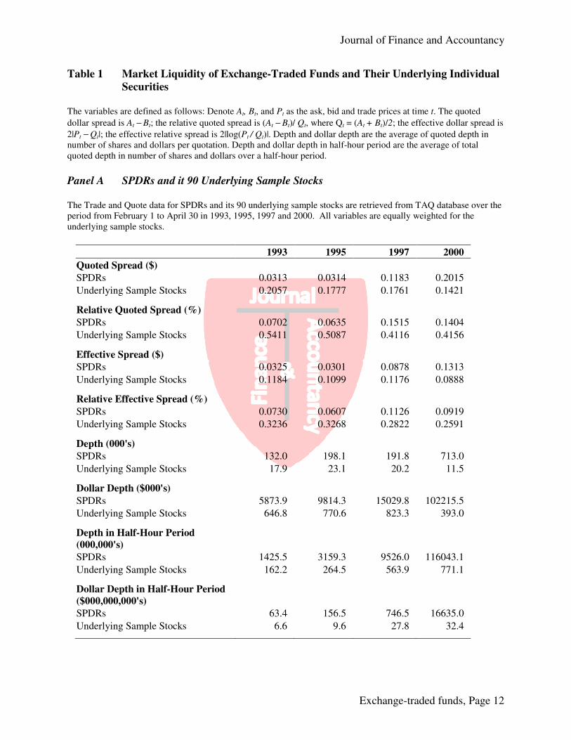
Table 1 Panel A reports the market liquidity for SPDRs and its 90 underlying sample stocks over the period of February 1 to April 30 in 1993, 1995, 1997 and 2000. During the time period of February 1 to April 30 in 1993, the three months right after the SPDRs was launched, the average quoted dollar spread, relative quoted spread, effective dollar spread and relative effective spread for SPDRs are $0.0313, 0.0702%, $0.0325, and 0.0730% respectively. For its underlying sample stocks, these variables are $0.2057, 0.5411%, $0.1184, and 0.3236% respectively. Apparently, the quoted and effective bid-ask spreads of SPDRs are much lower than its underlying .

During the period of February 1 to April 30 in 2000, the average quoted dollar spread and effective spread for SPDRs are $0.2015 and $0.1313, respectively. Unlike the three-month period in 1993, they are significantly higher than its underlying sample stocks’ average, which are equal to $0.1421 and $0.0888. But the SPDRs still has the much lower relative quoted spread and relative effective spread, which are 0.1404% and 0.0919%, than the sample average of 0.4200% and 0.255%. The reason is because the SPDRs’ trading price has increased remarkably from $44.56 to $142.92 from 1993 to 2000 and the average prices for its underlying sample stocks are almost same in 1993 and 2000.

In May and June of 1997, the AMEX and NYSE changed their minimum price increment from eighth to sixteenth. From the Table 1 Panel A, we can observe that the average spread for the sample stocks are lower in 2000 than in other periods, i.e. 1993, 1995 and 1997.

Besides the bid-ask spread, we also consider depth as another measurement of the market liquidity. There are four variables in calculating depth and they are average quoted depth in number of shares and dollars per quotation and the average of total quoted depth in number of shares and dollars over a half-hour period. The lower half part of Table 1 Panel A reports the results about quoted depth in these four variables for SPDRs and its underlying sample stocks. From the table, we can learn that the quoted depth of SPDRs is much higher than the underlying sample stocks’ average for all the periods, both in number of shares and dollars, and both for per quotation and half-hour period. And also, the quoted depth of SPDRs increases remarkably from 1993 to 2000 for all four variables, but underlying sample stocks only increases in half-hour quoted depth and there is no significant increase in quoted depth per quotation.

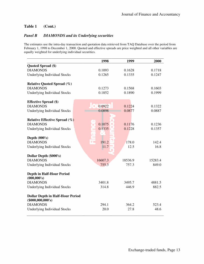
Table 1 Panel B reports the market liquidity for DIAMONDS and its underlying 30 stocks. Quite similar as SPDRs, DIAMONDS have a higher quoted and effective spread than the average of its underlying stocks when DIAMONDS have a higher price in year 1999 and 2000. And also quite similar as SPDRs, DIAMONDS have lower relative quoted and effective bid-ask price and have a much higher quoted depth, both in number of shares and dollars, and both for per quotation and half-hour period, when compare with its underlying stock average.

In summary, Table 1 indicates that there is a strong tendency for the market for ETFs to be more liquid than the market for its underlying individual stocks.

4.2. Adverse Selection Cost

Because there is less information asymmetry in markets for ETFs than in markets of their underlying individual securities, we predict that the adverse selection component of the bid-ask spread is lower for ETFs than their underlying individual securities. We choose Glosten and Harris (1988), and Lin, Sanger and Booth (1995)’s models to decompose the bid-ask spread for SPDRs, DIAMONDS and their underlying stocks. The estimation results are presented in Table 2 and Table 3.



Table 2 reports the estimation results by using Lin, Sanger and Booth (1995)’s model. This model measures the percentage adverse selection component of effective spread. The estimates for SPDRs and its underlying sample stocks are listed in Table 2 Panel A. Over the four three-month periods from 1993 to 2000, SPDRs has the adverse selection cost of 23.93%, 13.38%, 8.91%, 10.29% and the sample stocks have the average of 28.74%, 29.30%, 36.36%, 39.51%, respectively. SPDRs have lower adverse selection component than the average of the underlying sample stocks over all the periods. Compare the adverse selection cost between SPDRs and the summary statistics of 90 sample stocks, we also find the SPDRs’ adverse selection costs are even lower than the minimum of sample stocks in 1997 and 2000. In 1995, its adverse selection costs are located between the minimum and the first quartile of the sample stocks7.

Lin, Sanger and Booth (1995)’s model measures the percentage adverse selection component of effective spread. Multiplying this relative measurement by effective spread for each stock, we can get the absolute adverse selection cost in cents. The last two column of Table 2 Panel A reports this estimates and it shows that investors pay much lower adverse selection cost in trading SPDRs than in trading its underlying stocks, i.e. investor only pay 0.83¢ as adverse selection cost if they trade in SPDRs and they need to pay 3.69¢ on average if they trade in regular stocks.

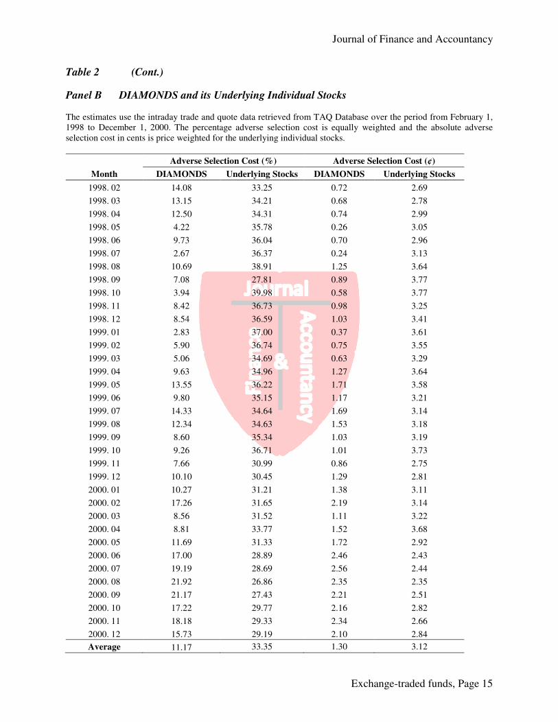
Table 2 Panel B lists the adverse selection cost for DIAMONDS and its underlying 30 stocks each month over the sample period from February 1998 through December 2000. On average, DIAMONDS have a relative adverse cost of 11.17%, which is much lower than the average of its underlying stocks, 33.35%. We also calculate the adverse selection cost in cents on portfolio level, i.e. the price weighted adverse selection cost for portfolio based on each stock’s adverse selection cost in cents and its price weight at the end of each month. The results are reported in the last two columns of Table 2 Panel B. Investors pay 1.30 ¢ adverse selection cost to trade in DIAMONDS and pay 3.12 ¢ for it underlying individual stocks.

Glosten and Harris (1988)’s model estimates the percentage adverse selection of the bid-

ask spread, )(2)(2)(2 ,1,0,1,0,1,0 iiiiiiiiii VzzVccVzzZ ++++= and the results are reported in

Table 3. In periods of 1993, 1997 and 2000, SPDRs have the adverse selection cost of 15.56%,

15.41% and 16.52%, which are significantly lower than sample average of 20.44%, 26.43% and 26.82%. In 1995, SPDRs have an adverse selection cost of 18.64%, which is little higher than the sample stocks’ average of 18.52%. Comparing the absolute adverse selection cost in cents, SPDRs cost investors much lower than its underlying sample stocks in all sample periods.

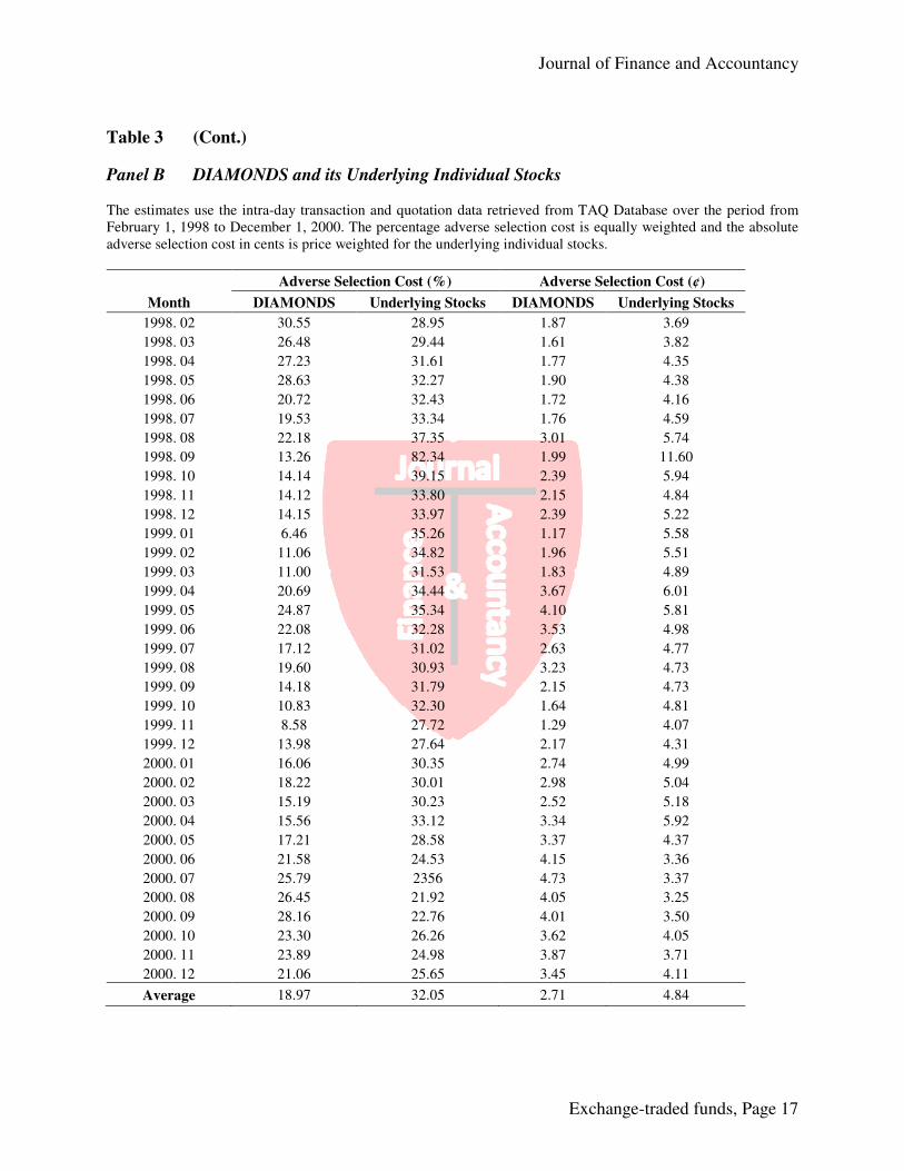
We also calculate the adverse selection costs for DIAMONDS and its underlying securities on portfolio level each month over the sample period from February 1998 through December 2000. Table 3 Panel B reports the results and shows that DIAMONDS have a lower adverse selection cost than its underlying stocks, both in relative and absolute measures.

In summary, all the empirical results of the bid-ask spread decomposition are consistent with our conjecture, i.e. ETFs have a lower adverse selection component compare with their underlying individual securities.

4.3. Trade Informativeness

7 The summary statistics of adverse selection component for SPDRs’ 90 sample stocks are available upon request, both for LSB and GH model.



Hasbrouck (1991b) develops two measures of trade informativeness. One is the trade-

correlated component of the variance of efficient price change, which has a natural interpretation as an absolute measure of trade informativeness. The other is the relative measure, which computed as the trade-correlate component of efficient price change variance divided by the total efficient price change variance.

We adopt a four-variable VAR and VMA model to estimate the trade informativeness, i.e. we use trade indicator, signed trading volume and signed squared trading volume as trade variables. The results are reported in Table 4. Panel A compares the estimates of SPDRs and its underlying sample stocks. SPDRs have trade informativeness of 1.57%, 1.65%, 3.30% and 3.45% over the period from February 1 to April 30 in 1993, 1995, 1997 and 2000, while its underlying sample stocks have 29.00%, 35.43%, 43.56% and 36.70% on average. SPDRs have much lower relative trade informativeness than its underlying stocks. Overall, we find that there is little private information impact on the SPDRs quote revision compare with the regular stocks. Thus, information asymmetry is lower in the market of SPDRs than in the market of its underlying securities.

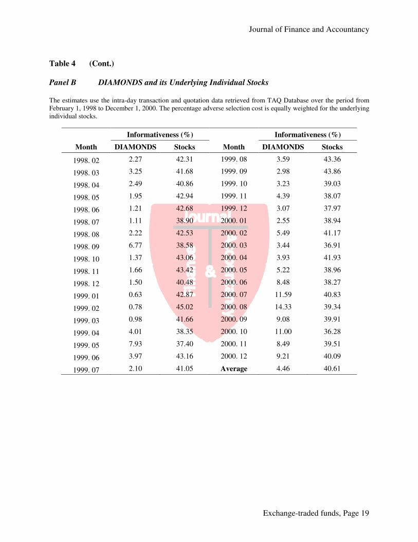
Panel B lists the results of DIAMONDS and its underlying securities each month over the sample period from February 1998 through December 2000. DIAMONDS have an average of 4.46% relative trade informativeness and its underlying stocks have the average of 40.61%.

In summary, the empirical results reported in Table 4 further confirm that the information asymmetry is lower in the market of ETFs because the trade informativeness is lower for ETFs than their underlying individual securities.

5. CONCLUSION

The popularity of ETFs in recent years raises the question that why this type of securities

attract so many investors, who obviously can choose buying and selling their underlying securities that compose the indexes in the same proportions to get the same cash flow. Subrahmanyam (1991) and Gorton and Pennacchi (1993) theoretically provide the reason why this type of securities exist and why they are popular. Due to the “diversification” or “information offset” effect, the introduction of the ETFs reduces the informed traders information advantage and the market maker would face less adverse selection problem in this market than in the market of individual securities. So the uninformed traders will lose less in their adverse trading with informed traders in this market and the discretionary uninformed traders tend to concentrate their trading in the market of ETFs. Based on Subrahmanyam (1991) and Gorton and Pennacchi (1993)’s model, we hypothesize that the information asymmetry is lower in the markets of ETFs than in the markets of individual securities. Use SPDRs and DIAMONDS as examples, we analyze the information asymmetry for ETFs and their underlying individual stocks.

We find that ETFs are more liquid, i.e. have narrower bid-ask spread and higher quoted depth. We then employ the Glosten and Harris (1988), and Lin, Sanger and Booth (1995)’s models to decompose the bid-ask spread and find that ETFs have lower adverse selection cost compare with individual securities. We further adopt Hasbrouck (1991a, 199b) Vector Autoregressive and Vector Moving Average model to estimate the informativeness of the trades and we find that the information content conveyed by the trades is less in the market of ETFs than in their individual securities both in absolute and relative measures.



References Ackert, L. F. & Tian, Y. S. (2000). Arbitrage and valuation in the market for Standard and Poor’s

Depository Receipts. Financial Management, 29, 71-88 Elton, E. J., Gruber, M. J., Comer, G., & Li, K. (2002). Spiders: where are the bugs? Journal of

Business, 75, 453-472. Glosten, L. R. & Harris, L. E. (1988). Estimating the components of the bid/ask spread. Journal

of Financial Economics, 21, 123-142 Gorton, G. B. & Pennacchi, G. G. (1993). Security baskets and index-linked securities. Journal

of Business, 66, 1-27 Hasbrouck, J. (1991). Measuring the information content of stock trades. The Journal of

Finance, 46, 179-207 Hasbrouck, J. (1991). The summary informativeness of stock trades: an econometric analysis.

The Review of Financial Studies, 4, 571-595 Huang, R. D. & Stoll, H. R. (1994). Market microstructure and stock return predictions. Review

of Financial Studies, 7, 179-213 Lee, C. M. C. & Ready, M. J. (1991). Inferring trade direction from intraday data. The Journal of

Finance, 46, 733-746 Lin, J., Sanger, G. C. & Booth, G. G. (1995). Trade size and components of the bid-ask spread.

Review of Financial Studies, 8, 1153-1183 Roll, R. (1984). A simple implicit measure of the effective bid-ask spread in an efficient market.

The Journal of Finance, 39, 1127-1139 Stoll, H. R. (1989). Inferring the components of the bid-ask spread: theory and empirical tests,

The Journal of Finance, 44, 115-134 Subrahmanyam, A. (1991). A theory of trading in stock index futures. Review of Financial

Studies, 4, 17-51 Van Ness, B., Van Ness, R. & Warr, R. S. (2001). How well do adverse selection components

measure adverse selection? Financial Management, 30, 5-30



Table 1 Market Liquidity of Exchange-Traded Funds and Their Underlying Individual Securities

The variables are defined as follows: Denote At, Bt, and Pt as the ask, bid and trade prices at time t. The quoted

dollar spread is At − Bt; the relative quoted spread is (At − Bt)/ Qt, where Qt = (At + Bt)/2; the effective dollar spread is

2|Pt − Qt|; the effective relative spread is 2|log(Pt / Qt)|. Depth and dollar depth are the average of quoted depth in number of shares and dollars per quotation. Depth and dollar depth in half-hour period are the average of total quoted depth in number of shares and dollars over a half-hour period.

Panel A SPDRs and it 90 Underlying Sample Stocks

The Trade and Quote data for SPDRs and its 90 underlying sample stocks are retrieved from TAQ database over the period from February 1 to April 30 in 1993, 1995, 1997 and 2000. All variables are equally weighted for the underlying sample stocks.

1993 1995 1997 2000

Quoted Spread ($)

SPDRs 0.0313 0.0314 0.1183 0.2015

Underlying Sample Stocks 0.2057 0.1777 0.1761 0.1421

Relative Quoted Spread (%)

SPDRs 0.0702 0.0635 0.1515 0.1404


Effective Spread ($)

SPDRs 0.0325 0.0301 0.0878 0.1313


Relative Effective Spread (%)

SPDRs 0.0730 0.0607 0.1126 0.0919


Depth (000's)

SPDRs 132.0 198.1 191.8 713.0


Dollar Depth ($000's)

SPDRs 5873.9 9814.3 15029.8 102215.5


Depth in Half-Hour Period (000,000's)

SPDRs 1425.5 3159.3 9526.0 116043.1


Dollar Depth in Half-Hour Period ($000,000,000's)

SPDRs 63.4 156.5 746.5 16635.0




Table 1 (Cont.) Panel B DIAMONDS and its Underlying securities The estimates use the intra-day transaction and quotation data retrieved from TAQ Database over the period from February 1, 1998 to December 1, 2000. Quoted and effective spreads are price weighted and all other variables are equally weighted for underlying individual securities.

1998 1999 2000

Quoted Spread ($)

DIAMONDS 0.1093 0.1628 0.1718

Underlying Individual Stocks 0.1265 0.1335 0.1247

Relative Quoted Spread (%)

DIAMONDS 0.1273 0.1568 0.1603


Effective Spread ($)

DIAMONDS 0.0922 0.1224 0.1322


Relative Effective Spread (%)

DIAMONDS 0.1075 0.1176 0.1236


Depth (000's)

DIAMONDS 191.2 178.0 142.4


Dollar Depth ($000's)

DIAMONDS 16607.3 18536.9 15283.4


Depth in Half-Hour Period (000,000's)

DIAMONDS 3401.8 3495.7 4881.5


Dollar Depth in Half-Hour Period ($000,000,000's)

DIAMONDS 294.1 364.2 523.4




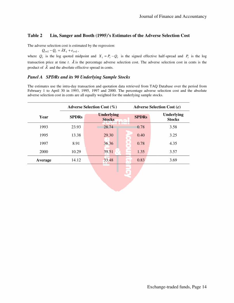
Table 2 Lin, Sanger and Booth (1995)’s Estimates of the Adverse Selection Cost The adverse selection cost is estimated by the regression:

11 ++ +=− tttt eXQQ λ ,

where tQ is the log quoted midpoint and ttt QPX −= is the signed effective half-spread and tP is the log

transaction price at time t. λ is the percentage adverse selection cost. The adverse selection cost in cents is the

product of λ and the absolute effective spread in cents.

Panel A SPDRs and its 90 Underlying Sample Stocks The estimates use the intra-day transaction and quotation data retrieved from TAQ Database over the period from February 1 to April 30 in 1993, 1995, 1997 and 2000. The percentage adverse selection cost and the absolute adverse selection cost in cents are all equally weighted for the underlying sample stocks.

Adverse Selection Cost (%) Adverse Selection Cost (¢)

Year SPDRs Underlying

Stocks SPDRs

Underlying Stocks

1993 23.93 28.74 0.78 3.58

1995 13.38 29.30 0.40 3.25

1997 8.91 36.36 0.78 4.35

2000 10.29 39.51 1.35 3.57

Average 14.12 33.48 0.83 3.69



Table 2 (Cont.)

Panel B DIAMONDS and its Underlying Individual Stocks The estimates use the intraday trade and quote data retrieved from TAQ Database over the period from February 1, 1998 to December 1, 2000. The percentage adverse selection cost is equally weighted and the absolute adverse selection cost in cents is price weighted for the underlying individual stocks.


Month DIAMONDS Underlying Stocks DIAMONDS Underlying Stocks

1998. 02 14.08 33.25 0.72 2.69

1998. 03 13.15 34.21 0.68 2.78

1998. 04 12.50 34.31 0.74 2.99

1998. 05 4.22 35.78 0.26 3.05

1998. 06 9.73 36.04 0.70 2.96

1998. 07 2.67 36.37 0.24 3.13

1998. 08 10.69 38.91 1.25 3.64

1998. 09 7.08 27.81 0.89 3.77

1998. 10 3.94 39.98 0.58 3.77

1998. 11 8.42 36.73 0.98 3.25

1998. 12 8.54 36.59 1.03 3.41

1999. 01 2.83 37.00 0.37 3.61

1999. 02 5.90 36.74 0.75 3.55

1999. 03 5.06 34.69 0.63 3.29

1999. 04 9.63 34.96 1.27 3.64

1999. 05 13.55 36.22 1.71 3.58

1999. 06 9.80 35.15 1.17 3.21

1999. 07 14.33 34.64 1.69 3.14

1999. 08 12.34 34.63 1.53 3.18

1999. 09 8.60 35.34 1.03 3.19

1999. 10 9.26 36.71 1.01 3.73

1999. 11 7.66 30.99 0.86 2.75

1999. 12 10.10 30.45 1.29 2.81

2000. 01 10.27 31.21 1.38 3.11

2000. 02 17.26 31.65 2.19 3.14

2000. 03 8.56 31.52 1.11 3.22

2000. 04 8.81 33.77 1.52 3.68

2000. 05 11.69 31.33 1.72 2.92

2000. 06 17.00 28.89 2.46 2.43

2000. 07 19.19 28.69 2.56 2.44

2000. 08 21.92 26.86 2.35 2.35

2000. 09 21.17 27.43 2.21 2.51

2000. 10 17.22 29.77 2.16 2.82

2000. 11 18.18 29.33 2.34 2.66

2000. 12 15.73 29.19 2.10 2.84

Average 11.17 33.35 1.30 3.12



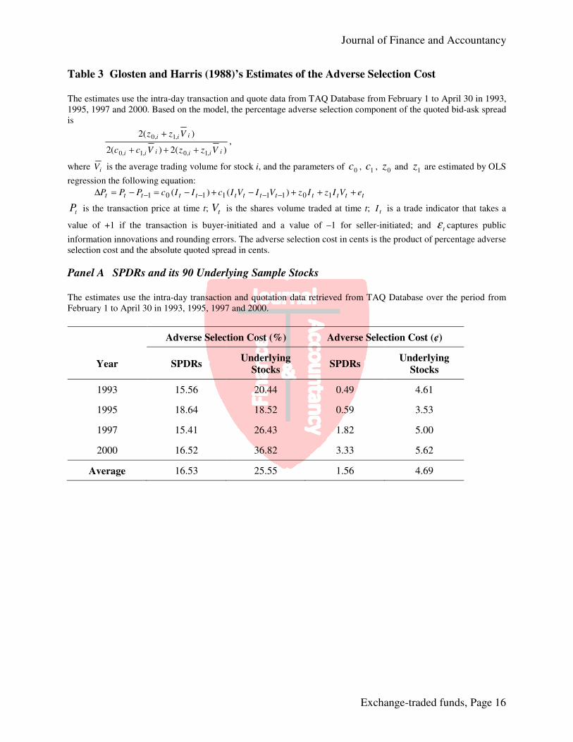
Table 3 Glosten and Harris (1988)’s Estimates of the Adverse Selection Cost The estimates use the intra-day transaction and quote data from TAQ Database from February 1 to April 30 in 1993, 1995, 1997 and 2000. Based on the model, the percentage adverse selection component of the quoted bid-ask spread is

)(2)(2

)(2

,1,0,1,0

,1,0

iiiiii

iii

VzzVcc

Vzz

+++

+,

where iV is the average trading volume for stock i, and the parameters of 0c , 1c , 0z and 1z are estimated by OLS

regression the following equation:

ttttttttttttt eVIzIzVIVIcIIcPPP +++−+−=−=∆ −−−− 10111101 )()(

tP is the transaction price at time t; tV is the shares volume traded at time t; tI is a trade indicator that takes a

value of +1 if the transaction is buyer-initiated and a value of –1 for seller-initiated; and tε captures public

information innovations and rounding errors. The adverse selection cost in cents is the product of percentage adverse selection cost and the absolute quoted spread in cents.

Panel A SPDRs and its 90 Underlying Sample Stocks

The estimates use the intra-day transaction and quotation data retrieved from TAQ Database over the period from February 1 to April 30 in 1993, 1995, 1997 and 2000.


Year SPDRs Underlying

Stocks SPDRs

Underlying Stocks

1993 15.56 20.44 0.49 4.61

1995 18.64 18.52 0.59 3.53

1997 15.41 26.43 1.82 5.00

2000 16.52 36.82 3.33 5.62

Average 16.53 25.55 1.56 4.69



Table 3 (Cont.)

Panel B DIAMONDS and its Underlying Individual Stocks The estimates use the intra-day transaction and quotation data retrieved from TAQ Database over the period from February 1, 1998 to December 1, 2000. The percentage adverse selection cost is equally weighted and the absolute adverse selection cost in cents is price weighted for the underlying individual stocks.


Month DIAMONDS Underlying Stocks DIAMONDS Underlying Stocks

1998. 02 30.55 28.95 1.87 3.69

1998. 03 26.48 29.44 1.61 3.82

1998. 04 27.23 31.61 1.77 4.35

1998. 05 28.63 32.27 1.90 4.38

1998. 06 20.72 32.43 1.72 4.16

1998. 07 19.53 33.34 1.76 4.59

1998. 08 22.18 37.35 3.01 5.74

1998. 09 13.26 82.34 1.99 11.60

1998. 10 14.14 39.15 2.39 5.94

1998. 11 14.12 33.80 2.15 4.84

1998. 12 14.15 33.97 2.39 5.22

1999. 01 6.46 35.26 1.17 5.58

1999. 02 11.06 34.82 1.96 5.51

1999. 03 11.00 31.53 1.83 4.89

1999. 04 20.69 34.44 3.67 6.01

1999. 05 24.87 35.34 4.10 5.81

1999. 06 22.08 32.28 3.53 4.98

1999. 07 17.12 31.02 2.63 4.77

1999. 08 19.60 30.93 3.23 4.73

1999. 09 14.18 31.79 2.15 4.73

1999. 10 10.83 32.30 1.64 4.81

1999. 11 8.58 27.72 1.29 4.07

1999. 12 13.98 27.64 2.17 4.31

2000. 01 16.06 30.35 2.74 4.99

2000. 02 18.22 30.01 2.98 5.04

2000. 03 15.19 30.23 2.52 5.18

2000. 04 15.56 33.12 3.34 5.92

2000. 05 17.21 28.58 3.37 4.37

2000. 06 21.58 24.53 4.15 3.36

2000. 07 25.79 2356 4.73 3.37

2000. 08 26.45 21.92 4.05 3.25

2000. 09 28.16 22.76 4.01 3.50

2000. 10 23.30 26.26 3.62 4.05

2000. 11 23.89 24.98 3.87 3.71

2000. 12 21.06 25.65 3.45 4.11

Average 18.97 32.05 2.71 4.84



Table 4 Trade Informativeness of Exchange-Traded Funds and Their Underlying

Individual Stocks

Trade informativeness is computed as 22, wxw σσ , where 2

wσ is the variance of efficient price change and 2,xwσ is

trade-correlated component of 2wσ . They are defined as

21

210

1

10

0

10

0

2 )1()()( σσ ⋅∑++∑′

Ω∑==

∗

=

∗

=

∗

ti

ti

tiw abb and )()(

10

0

10

0

2, ∑

′Ω∑=

=

∗

=

∗

ti

tixw bbσ

where ∗∗ii ba , and 2

1 ,σΩ are come from the Hasbrouck (1991a, 1991b)’s VAR and VMA model:

tttttt

tttttt

xdxdrcrcx

xbxbrarar

,222112211

,11102211

υυ++++++=

++++++=

−−−−

−−−

LL

LL

LL

LL

++++++=

++++++=

−∗

−∗

−∗

−∗

−∗∗

−∗

−∗

2,221,21,22,121,11

1,21,202,121,11,1

tttttt

tttttt

ddccx

bbaar

υυυυυ

υυυυυ

where )/log(100 1−×= ttt qqr , tq is the quote midpoints; tx is the trade variable column vector [ ]210ttt xxx ,

where 0tx is trade indicator (+1 if the market order is a purchase and -1 if a sale), 1

tx is signed trading volume in 100

shares (positive if the market order is a purchase and negative if a sale), and 2tx is signed square of 1

tx . VAR is

truncated at lag 5 and VMA is truncated at lag 10.

Panel A SPDRs and its 90 Underlying Sample Stocks The estimates use the intra-day transaction and quotation data retrieved from TAQ Database over the period from February 1 to April 30 in 1993, 1995, 1997 and 2000.

Trade informativeness (%)

Year SPDRs Underlying stocks

Mean Minimum 1st Quartile Median 3rd Quartile

Maximum

1993 1.57 29.00 0.61 20.26 28.76 36.62 64.99

1995 1.65 35.43 2.31 29.67 36.46 41.46 53.39

1997 3.30 43.56 1.46 38.79 43.43 48.70 73.46

2000 3.45 36.70 13.00 32.35 37.27 41.88 56.76



Table 4 (Cont.) Panel B DIAMONDS and its Underlying Individual Stocks The estimates use the intra-day transaction and quotation data retrieved from TAQ Database over the period from February 1, 1998 to December 1, 2000. The percentage adverse selection cost is equally weighted for the underlying individual stocks.

Informativeness (%) Informativeness (%)

Month DIAMONDS Stocks Month DIAMONDS Stocks

1998. 02 2.27 42.31 1999. 08 3.59 43.36

1998. 03 3.25 41.68 1999. 09 2.98 43.86

1998. 04 2.49 40.86 1999. 10 3.23 39.03

1998. 05 1.95 42.94 1999. 11 4.39 38.07

1998. 06 1.21 42.68 1999. 12 3.07 37.97

1998. 07 1.11 38.90 2000. 01 2.55 38.94

1998. 08 2.22 42.53 2000. 02 5.49 41.17

1998. 09 6.77 38.58 2000. 03 3.44 36.91

1998. 10 1.37 43.06 2000. 04 3.93 41.93

1998. 11 1.66 43.42 2000. 05 5.22 38.96

1998. 12 1.50 40.48 2000. 06 8.48 38.27

1999. 01 0.63 42.87 2000. 07 11.59 40.83

1999. 02 0.78 45.02 2000. 08 14.33 39.34

1999. 03 0.98 41.66 2000. 09 9.08 39.91

1999. 04 4.01 38.35 2000. 10 11.00 36.28

1999. 05 7.93 37.40 2000. 11 8.49 39.51

1999. 06 3.97 43.16 2000. 12 9.21 40.09

1999. 07 2.10 41.05 Average 4.46 40.61

exchange-traded funds and information asymmetry · journal of finance and accountancy...

Documents