measuring financial advice: aligning client elicited and
TRANSCRIPT

Measuring Financial Advice: aligning clientelicited and revealed risk
John R.J. Thompson, Longlong Feng, R. Mark Reesor,Chuck Grace, and Adam Metzler
Department of MathematicsWilfrid Laurier University
Waterloo, Ontario, Canada N2L 3C5
May 26, 2021
Abstract
Financial advisors use questionnaires and discussions with clients to determine a suitable port-folio of assets that will allow clients to reach their investment objectives. Financial institutionsassign risk ratings to each security they offer, and those ratings are used to guide clients andadvisors to choose an investment portfolio risk that suits their stated risk tolerance. This papercompares client Know Your Client (KYC) profile risk allocations to their investment portfoliorisk selections using a value-at-risk discrepancy methodology. Value-at-risk is used to measureelicited and revealed risk to show whether clients are over-risked or under-risked, changes inKYC risk lead to changes in portfolio configuration, and cash flow affects a client’s portfoliorisk. We demonstrate the effectiveness of value-at-risk at measuring clients’ elicited and re-vealed risk on a dataset provided by a private Canadian financial dealership of over 50, 000accounts for over 27, 000 clients and 300 advisors. By measuring both elicited and revealed riskusing the same measure, we can determine how well a client’s portfolio aligns with their statedgoals. We believe that using value-at-risk to measure client risk provides valuable insight toadvisors to ensure that their practice is KYC compliant, to better tailor their client portfoliosto stated goals, communicate advice to clients to either align their portfolios to stated goals orrefresh their goals, and to monitor changes to the clients’ risk positions across their practice.
Keywords: Risk measures, Value-at-risk, Portfolio management, Financial advice, Client-advisor relationship
1
arX
iv:2
105.
1189
2v1
[ec
on.E
M]
25
May
202
1

John R.J. ThompsonDepartment of MathematicsWilfrid Laurier UniversityWaterloo, Ontario N2L [email protected]
Longlong FengDepartment of MathematicsWilfrid Laurier UniversityWaterloo, Ontario N2L [email protected]
R. Mark ReesorDepartment of MathematicsWilfrid Laurier UniversityWaterloo, Ontario N2L [email protected]
Chuck GraceDepartment of FinanceIvey Business SchoolLondon, Ontario N6G [email protected]
Adam MetzlerDepartment of MathematicsWilfrid Laurier UniversityWaterloo, Ontario N2L [email protected]
2

1 Introduction
In previous research, we find that that Know Your Client (KYC) information–such as gender,
residence region, and marital status–does not explain client investment behaviours, whereas
eight variables for trade and transaction frequency and volume are more informative (Thompson
et al., 2021). With these findings that trading behaviour (recency and volume patterns) is
linked to actual client risk preference and capacity, our recommendation to financial regulators
and advisors is to use metrics more advanced than those gleaned from KYC information to
understand clients better. The dataset used in that paper spanned from January 1st 2019
to August 12th 2019, and consisted of daily KYC information (age, gender, annual income,
risk tolerance) and financial information (account type, total value of that account, proportion
of total value invested into different securities) for 50, 980 accounts of 27, 644 clients and 311
advisors.
This paper demonstrates how value-at-risk (VaR) can be used as an advanced metric by
financial advisors to manage their clients’ portfolio risks. We show that VaR provides unique
real-time empirical insights that can help stakeholders visualize gaps between the elicited KYC-
derived profile risk and the actual portfolio risk revealed by trading behaviours. We examine
how clients’ trading behaviour and cash flow impact their portfolios and use VaR to quantify
how much of each client’s portfolio is genuinely “at risk” and how far clients are from their
stated risk preferences. While part of our contribution to the literature is a methodology to
estimate clients’ risk preferences, our primary contribution is a methodology to measure the
difference in elicited and revealed risk tolerance.
In Canada, financial advisors and dealers are required by provincial securities commissions
and self-regulatory organizations to collect and maintain KYC information for investor ac-
counts. With this information, investors, under their advisor’s guidance, decide on investments
that are presumed to be beneficial to their investment goals and therefore suitable. Suitabil-
ity is described by regulators in Canada as a “meaningful dialogue with the client to obtain
a solid understanding of the client’s investment needs and objectives . . .” (Ontario Securities
Commission, 2014), and has been updated to better serve client needs (Ontario Securities Com-
3

mission, 2019). The assumption is that any investment purchases or sales (trading behaviour)
will conform to the KYC attributes and therefore be suitable.
It should be noted that suitability must be informed by both Know Your Product (KYP) and
KYC attributes. Part of the KYP information on securities made available by the dealership is a
risk rating (Ontario Securities Commission, 2009). These risk ratings are used to place products
into risk buckets (for example, low, medium, or high risk). The KYC attributes give a portfolio
selection across risk buckets, followed by a selection of products within each risk bucket. Our
analysis evaluates a client’s portfolio based on their KYP attributes–at least in terms of their
risk and return characteristics. Our measures do not delve deeper to complete comprehensive
due diligence of the investment products as would be prescribed by the regulators.
Our analysis shows that advisors and clients use the KYC prescribed risk as a ”guard rail”
against which they define–and do not generally exceed–upper and lower boundaries. However,
between the ”guard rails”, they tailor and customize portfolios in a manner that is consistent
with their clients’ elicited KYC risks. Do our findings suggest negative consequences for in-
vestors? We find that advisors are systemically safe and conservative and thus do not appear
to expose clients to undue risk. For clients seeking to preserve capital, that is good news, but
clients seeking to maximize growth may not be exposed to enough risk to achieve their expressed
goals. Under-risked accounts are just as problematic as over-risked, but easier for advisors to
defend to regulators and lawyers given there is no significant loss of funds. An example might
be older clients who can preserve their capital but are unable to achieve investment incomes
that allow them to maintain their lifestyles. An accurate answer to the question of client impact
can only be answered through the lens of the advisor/client interactions–which are by necessity
private and confidential.
Every client has a unique story, and we present methods that can digitize their story to
improve personalization, transparency, timeliness and visualization. Our methodology falls into
the interest realms of advisors, regulators, and robo-advisors; (1) advisors can implement these
mathematical methods into their practice1, (2) regulators will be able to identify inconsisten-
1We have included an example Excel spreadsheet as part of this article, and this sheet is available uponrequest from the corresponding author.
4

cies in practitioners’ portfolios, and (3) robo-advisors can use these methods to help advisors
monitor their clients’ portfolios.
The paper from here unfolds as such: Section 2 provides the academic context for our
methodology in the broad area of measuring risk tolerance. Section 3 is an overview of the
dataset provided by a private Canadian financial dealership. Section 4 is a study of financial
methodologies, including VaR, to measure the discrepancy between profile and portfolio risk.
Section 5 shows the results of using the VaR methodology for measuring and comparing risk
for clients, advisors, and dealerships. Lastly, Section 6 summarizes our results and provides a
broader discussion for the impacts of the methodology presented herein.
2 Context
One goal of this paper is to bridge the gap between the ivory tower of academic computational
behavioural finance and the real work of the financial agent–a client, advisor, dealership, regu-
lator, or otherwise. This section provides the academic context of how behavioural finance has
been applied to understand risk tolerance from questionnaires and trading behaviour, point
to real applications of behavioural concepts that have directly benefited practitioners, and
elaborate on how our work is helpful to both academics and practitioners.
2.1 Behavioural finance: elicited and revealed risk
In behavioural economics, there is a large body of research dedicated to measuring and under-
standing the difference between elicited and revealed preferences of consumers, originated by
Samuelson (1948). In essence, elicited preferences are what people say they prefer, whereas re-
vealed preferences are what they actually prefer, as shown through their behaviours. To apply
this concept in finance, elicited and revealed preferences for financial risk were developed, with
focuses on estimating the utility of wealth of consumers based on their investing behaviour
(Dybvig and Rogers, 1997), applications of prospect theory (Kahneman and Tversky, 2013),
understanding the perceptions of risk (Diacon and Ennew, 2001), the effect of cognitive abil-
ity on risk preferences (Guillemette et al., 2015), and–the focus of this paper–measuring risk
5
preferences.
Elicited risk in investment dealerships is typically collected via questionnaires adminis-
tered in-person yearly by financial advisors to clients. In conjunction with the conversations
surrounding the questionnaire, the responses to the questionnaire are used to calculate risk
preferences. Finke and Guillemette (2016) provides a modern review of eliciting risk tolerance
from questionnaires; their summative findings include measuring choices surrounding income
risk and volatility to assess risk tolerance (Guillemette et al., 2012), financial literacy effects
on risk assessment (Linciano and Soccorso, 2012), and emotional responses to risk and loss
aversion (Loewenstein et al., 2001; Grable and Lytton, 2001; Michael et al., 2015). Wahl and
Kirchler (2020) employed a modern questionnaire methodology that measures risk propensity,
attitude, capacity, and knowledge to elicit risk tolerance from clients. Our dataset described in
Section 3 contains the risk elicited using a questionnaire under the KYC obligation guidelines.
A risk score is determined from the questionnaire’s responses by calculating a weighted sum
based on their answers. That risk score is then transformed by the advisor administering the
questionnaire into a profile risk allocation (percentage of assets allocated across risk buckets).
Detailed questionnaire response data is hitherto unavailable, with future plans to exchange and
analyze that information with our industry partner to better evaluate a client’s elicited risk
with guidance from revealed risk.
Revealed risk is typically measured by a client’s recovered utility of wealth from their trade
and transaction behaviours. Utility of wealth is the idea that income and total wealth affect
how a loss is perceived; for example, a $10, 000 loss is significant if your total wealth is $50, 000
and insignificant if your total wealth is $50 million. This concept is not new; income and total
wealth have been shown to affect risk tolerance based on the utility of wealth(Samuelson, 1975).
A client’s utility of wealth can be recovered from realizations of how they are investing their
wealth (Dybvig and Polemarchakis, 1981; Dybvig and Rogers, 1997).
We apply the financial measure of VaR to evaluate both elicited and revealed risk individ-
ually. VaR is a quantile of the profit-and-loss distribution–for example, fixing a time horizon
of one year, the 99% VaR is the minimum loss you should expect on your worst day out of one
6
hundred. This concept is well-known in financial management, where it is explained in depth in
Jorion (2007) with many different strategies for implementation (Kuester et al., 2006). In this
paper, VaR is used to accomplish three tasks: (1) quantify elicited risk, (2) quantify revealed
risk, and (3) quantify the discrepancy between elicited and revealed risk.
Previous research bridging the gap between elicited and revealed has been conducted to
understand risk preferences for crop producers (Sharma and Schoengold, 2016). Corter and
Chen (2006) used a weighted sum score methodology to measure revealed risk and compared
it with elicited risk measured with scores from a risk tolerance questionnaire. They found that
higher risk preferences in the questionnaire were positively correlated with higher risk sum
scores. However, our interest is not in reaffirming the correlation between elicited and revealed
risk but in quantifying the difference between the elicited and revealed preferences. In our
approach, VaR is a risk comparison methodology that allows the user to calculate elicited and
revealed risk using the same criteria for comparison. While part of our contribution to the
literature is using VaR to estimate clients’ risk preferences, our main contribution is measuring
the difference in elicited and revealed risk tolerance.
3 Data description
The dataset used in this paper is drawn from the same database provided by a private invest-
ment dealership discussed in Thompson et al. (2021). The dataset in this paper spans from
March 29th 2019 to August 12th 2019, and consists of daily KYC information (age, gender,
annual income, risk tolerance) and financial information (account type, total value of that ac-
count, proportion of total value invested into different securities) for 50, 980 accounts of 27, 644
clients and 311 advisors. The KYC information is collected via a questionnaire when the ac-
count is opened and is updated at least yearly, and the financial information is updated each
business day. All identifying data has been anonymized, and individuals will not be identified
or referenced in this paper. Also, any subset of the data cannot be publicly shared. Table 1
shows the variables of the data from Thompson et al. (2021) that are considered in this paper.
7

Table 1: Dataset details on clients’ KYC information.
Variable Summary Data type Example valuesAccounttype
Canadian account classifications that havedifferent benefits
Categorical Cash, LIRA, RDSP,RESP, RIF, RSP,TFSA, Margin2
Advisorytype
Where the advisor has the discretion to tradefor the client
Categorical Discretionary, non-discretionary, orunknown
Age Ages range from 18 to 98 years old, with av-erage at 57.4 years
Continuous 31 years old
Annual in-come
Gross annual income in CAD Continuous Multiples of $100between $0 and$15, 000, 000 inclusive
Gender 50.5% male and 49.5% female Indicator M,FInvestmentknowledge
The self-reported investment knowledge of2.5% sophisticated, 44.7% good, 35.2% fair,or 17.6% poor
Ordinal 1, 2, 3, or 4
Maritalstatus
67% married, 18% single, 11% unknown and4% divorced
Categorical M,D,S, or *
Number ofaccounts
Clients can have more than one account Ordinal 1,2,3,. . . 8
Residency Province or Country or Region, with approx-imately 65% from Ontario
Categorical ON, MB, AB, . . .
Retirementindicator
The client’s retirement status with 73.9% notretired, 18.2% retired, and 7.9% unknown
Indicator Yes, No
8

The new data in this paper that was previously unavailable is the discretionary information
of the client-advisor relationship. Advisors associated with the investment dealership have
direct control over the securities owned in each account. Clients cannot make direct changes
to the accounts without going through their financial advisor. There are two types of advisory
relationships: (i) advisors have full discretion on trading for the client’s accounts, or (ii) advisors
must have trades approved by the client. In our dataset, there are 4, 423 discretionary accounts,
44, 712 non-discretionary accounts, and 1, 845 unknown. Additionally, there exist accounts in
the dataset that the advisor personally owns, but that information is currently unavailable due
to anonymization. Henceforth, we will treat advisor accounts as client accounts since we are
informed that the dealership expects advisors to trade on their accounts, similar to how they
would trade for their clients. In fact, internal auditors at the dealership monitor advisor trades
to ensure that they are offering trades to or conducting trades for clients before trading the
same securities in the advisor’s personal accounts, where regulators mandate this behaviour.
The distribution of account residency is shown in Table 2, with the majority of accounts
owned by clients in the province of Ontario. Figure 1 shows a graph of the annual incomes
where we can see that 25% of all clients earn $37, 000 or less, 50% earn $64, 000 or less, and
75% earn $100, 000 or less. There are income spikes at multiples of $50k, and there were also
286 clients that earned $500, 000 or more. Figure 2 shows the total market values of client
portfolios, where 25% of all clients own assets valued at $44, 041 or less, 50% earn $113, 147 or
less, and 75% earn $262, 099 or less.
Table 2: Distribution of residency for client accounts. Locations are Ontario (ON), BritishColumbia (BC), Alberta (AB), Manitoba (MB) and Nova Scotia (NS).
Location ON BC AB MB NS OtherPercentage 65.36 13.85 12.80 4.07 2.17 1.75
Figure 3 shows clients’ ages, where the distribution is unimodal, centred at 57.5 years, has
a standard deviation of 14.8 years, and is very slightly left-skewed. The minimum age is 18
years–the legal age to open an account in Canada–and the maximum is 104. Table 3 shows
2Account types are cash, locked-in retirement account (LIRA), registered disability savings plan (RDSP),registered education savings plan (RESP), retirement income fund (RIF), retirement savings plan (RSP), tax-free savings account (TFSA), and margin accounts.
9

Figure 1: The distribution of annual incomes for clients on August 12th 2019, with a binwidth of$10, 000. The three vertical dashed lines represent the 25th, 50th, and 75th percentiles. Thereare 286 clients not pictured with annual incomes greater than $500, 000, with a maximumannual income of $15, 000, 000.
Figure 2: The distribution of the total market value for client portfolios on August 12th 2019,with a binwidth of $10, 000. There are 74 clients not pictured with portfolio market valuesgreater than $3, 000, 000, with a maximum of $62, 684, 999.
10

Figure 3: The distribution of client ages, where each bin contains one year.
the number of accounts for clients, where 77.3% of clients have two or fewer accounts. Table
4 shows the account types, where most own RSP and TFSA accounts. In addition, we also
Table 3: The number of accounts owned by clients.
Unique accounts 1 2 3 4 5 6 7 8Number of clients 13112 8246 4380 1457 330 87 20 12
Table 4: Distribution of account types.
Account type Cash LIRA RDSP RESP RIF RSP TFSA MarginNumber of accounts 7843 129 204 2975 6169 19, 979 11, 080 944
have data on the elicited and reveal risk distributions. This data is either collected during the
KYC questionnaire (elicited) or observed from trading behaviours (revealed), and is discussed
in the next section.
3.1 Profile risk allocation and portfolio risk selection
The dealer’s method to satisfy the KYC risk tolerance obligation results in their clients’ risk
tolerance represented as a set of five percentages, with each percentage associated with the
following categories: low, low-medium, medium, medium-high, and high risk. The percentages
11

sum to 100, so all risk tolerance is allocated. From here on, we will refer to these percentages,
elicited from a client, as the profile risk allocation, or simply profile risk. Each security available
for purchase from the dealer is evaluated to have a KYP risk rating classified into one of the
five risk categories. An investor’s familiarity with a security’s brand plays a key role in the
optimism of the financial return of an investment in that security (Aspara, 2013), and unfamiliar
securities have a higher perception of risk with lower return (Ganzach, 2000). Security risk
ratings provide numerical guidance to investors on the realistic risk of an investment. Our
dataset’s risk ratings are based on a weighting of the standard deviation of the security price,
maximum drawdown, downside deviation, and correlations with other securities. In this paper,
the revealed risk distribution on any given day is the percentage of total market value held in
each of the five risk categories. Henceforth, it will be referred to as the portfolio risk selection,
or simply portfolio risk.
3.2 Clusters
Our previous work grouped client behaviours–measured by a recency, frequency, monetary and
profile (RFMP) model–though a k-prototypes machine learning clustering algorithm (Thomp-
son et al., 2021). In that work, we found the optimal number of clusters to be five using
the silhouette coefficient and the Davies–Bouldin (DB) score. The cluster attributes yield five
personas:
• Cluster 1 – active investors who trade frequently, in large amounts and appear sensitive
to market influences,
• Cluster 2 – younger savers who make regular, smaller deposits using automated platforms
such as preauthorized chequing (PACs) and dollar cost averaging,
• Cluster 3 – “just in time” traders who make infrequent trades at seemingly random
intervals,
• Cluster 4 – older investors who make regular withdrawals and cash out dividends and
interest payments, and
12
• Cluster 5 – systematic savers who make larger trades but make use of automation for
predictable deposits and re-balancing.
In this paper, we further analyze those clusters to investigate whether the methodologies pre-
sented herein agree with our previous work. We note that risk tolerance was not an input
into the clustering algorithm, and previous analysis on the profile risk allocation of the clusters
showed little difference between clusters.
4 Methodology
Advisors allocate their clients’ wealth to different recommended proportions of risk categories,
and they select particular assets within these categories. Once set up, advisors continuously
aid clients in modifying their portfolio as markets evolve, based on their stated financial goals.
Advisors strive to construct portfolios that are consistent with stated goals, and thus one should
be able to quantify how close an advisor is coming to the stated goal. Otherwise, stated goals
are inconsequential. Advisors pick assets that are classified into risk categories–mandatory for
all financial institutions. In our dataset, each asset is classified into one of five risk categories.
It is natural to assume that when an advisor sets up a clients’ proportional risk allocation, the
advisor will ensure that their assets line up with that risk allocation.
A main issue is quantifying the difference between (i) a client’s prescribed KYC profile
risk and (ii) their actual portfolio risk. A risk allocation or selection is represented by an
ordered collection of five percentages associated with each risk category (Low, Low-medium,
Medium, Medium-high, High), where the percentages sum to one. An example portfolio risk
selection is (0.2, 0.1, 0.7, 0, 0) with 20% of wealth allocated to the low risk bucket, 10%
to low-medium, and 70% to medium. Readers familiar with linear algebra might (correctly)
recognize that we can view an allocation or selection as a point in five-dimensional Euclidean
space. In this case, quantifying discrepancy is as simple as computing the Euclidean distance
between two points. Readers familiar with probability theory might (correctly) recognize that
we can view an allocation or selection as a probability distribution, in which case quantifying
discrepancy would be possible using well-known measures such as Kullback-Liebler Divergence.
13

Unfortunately, neither of these approaches leads to meaningful comparisons to advisors or their
clients. See Appendix A for a detailed investigation of metrics and divergences used for risk
category comparisons. In other words, measuring the discrepancy in a mathematically valid way
is straightforward, but doing so in a manner that is both mathematically valid and financially
meaningful, is surprisingly non-trivial.
The well-known financial risk measure Value-at-Risk (VaR) allows us to evaluate and com-
pare risk allocations and selections in a valid and financially informative way. VaR captures
the risk tolerance relative to actual market indices, while also incorporating the relative and
correlated risk between risk categories. Typically, VaR is quoted in basis points (bps) so that
VaR across clients with different total market values can be compared. VaR can provide an
actual dollar value estimate of the minimum a client should expect to lose on their worst day
out of one hundred, which is an excellent communication tool between advisors and clients.
To compare profile and portfolio risk, the first step is to estimate the VaR and the second
step is to compute the difference in VaRs to compare them. Estimating VaR requires an
understanding of the assumptions on how the investor and advisor interpret each risk category,
and the statistical properties of the returns of those risk categories. Our analysis makes specific
choices to calculate VaR, but it is essential to highlight that the VaR framework is highly
customizable by the user.
4.1 Value-at-risk
Using the assets in a portfolio is necessary for the exact calculation of portfolio VaR. How-
ever, this approach fails for assigning a profile risk VaR–perceptions and securities held across
advisors can be very different. Our solution to calculating profile VaR similarly across clients
and advisors is to use an exchange-traded fund (ETF) as a representative investment for each
risk category. This methodology is customizable to any set of ETFs or any assets of the
user’s choosing. The risk representative iShares ETFs3 from a given class that had the longest
publicly-available data4 are shown in Figure 4 with their expected annualized returns, volatility,
3https://www.blackrock.com/ca/investors/en/products/product-list4https://ca.finance.yahoo.com
14

and correlations5.
The expected annualized return of each ETF and the correlations between them are used
to calculate VaR. The VaR calculation gives the minimum expected loss in basis points (bps)
on the worst trading day out of one hundred. Figure 4 shows an example VaR calculation for a
single client that is considering two possible portfolio selections. The client has a profile risk of
100% low-medium, and their risk is a loss of at least 10.91% of their total market value. They
are considering a portfolio VaR of 100% low, which yields a VaR of -0.23%–negative means
that on your worst day out of one hundred, you expect to gain 0.23% or less–and a 100% high
account, which yields 31.18% VaR. The discrepancy between the low and low-medium accounts
is -11.14%, and between low and high accounts is 20.27%. A negative VaR discrepancy means
the portfolio is relatively under-risked and a positive VaR discrepancy means it is relatively
over-risked.
5 Results
In this section, we apply our risk comparison methodology to a real trade and transaction
dataset. We show the benefits and drawbacks of using VaR to evaluate and compare profile
and portfolio risk. We start by investigating a single client’s performance over time, followed by
an advisor’s portfolio with a large clientele, and conclude with results at the financial dealership
level.
5.1 Client level
First, we look at how the two methodologies can evaluate the difference between the client’s
profile and portfolio risk. This investigation will show not only the usefulness of the VaR
methodology, but also show possible analyses and visualizations that could appear on a client
dashboard. The example client is a 62-year-old investor with five accounts with five types:
Cash, retirement savings plan (RSP), retirement income fund (RIF), tax-free savings account
5We have included an Excel spreadsheet (Microsoft Corporation, 2021) that reproduces the VaR calculation,and Appendix B that provides mathematical details of the calculation.
15

Figure 4: VaR calculation using Excel spreadsheet software. The spreadsheet is available toreaders.
16

Figure 5: The portfolio market value of each account of the example client over time.
(TFSA), registered education savings plan (RESP). The holdings of each account over time is
shown in Figure 5, where the account starts with approximately $300, 000 in their RIF accounts,
$75, 000 in each of their TFSA and RESP accounts, and change in each of their RIF, RSP, and
Cash accounts. A large addition of approximately $600, 000 is made in the fourth week of July
to their Cash account. Table 5 shows the market value, profile VaR, portfolio VaR, and VaR
discrepancy for each account on on August 12th 2019, where we can see they have the same
KYC profile risk (100% medium) across accounts. The accounts are all under-risked to their
stated goal, shown by the negative differences in VaR.
Table 5: The example client market values, profile VaR, portfolio VaR, and VaR discrepancyon August 12th 2019 by account type. The averages in the last row are weighted by the marketvalue of each account’s holdings.
Account Market Value (CAD) Profile VaR (bps) Portfolio VaR (bps) VaR discrepancy (bps)A1: Cash 595152 1216 971 -244A2: RSP 9883 1216 1089 -126A3: RIF 288552 1216 882 -333A4: TFSA 82302 1216 1089 -126A5: RESP 67028 1216 1089 -126Average 208583 1216 965 -251
Figure 6 shows the client’s profile VaR, individual account portfolio VaRs, and an overall
17

Figure 6: The example client’s account portfolio VaRs over time, with constant profile VaR of1216 bps for all accounts. The unseen TFSA account line is same as the RESP line.
portfolio VaR (weighted by market value) over time. Similar to their account holdings in Figure
5, we see there is a re-balancing of asset risks in their cash and RIF accounts, which affects
their overall portfolio average.
5.2 Advisor level
From the individual client view perspective, our methodology allows advisors to gain insight
into their clients’ risk positions and easily compare to their preferences. In addition, advisors
can gain insights on all clients across their firms by looking at the average metrics across clients
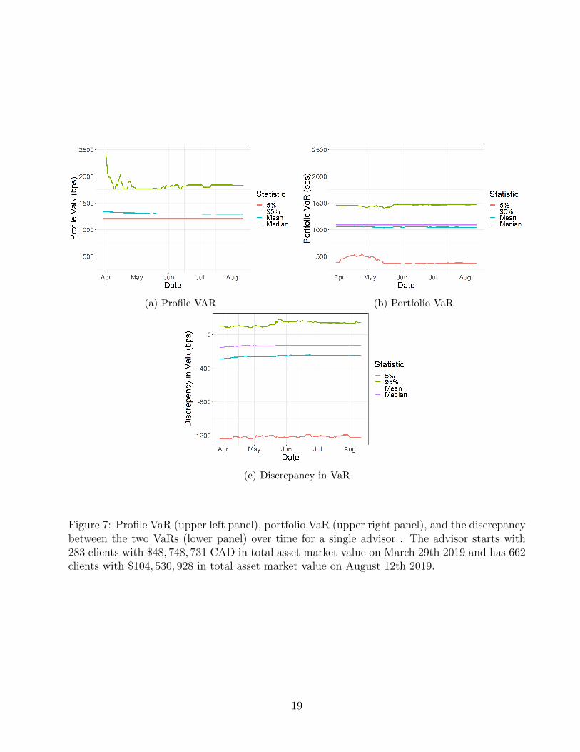
and the variation of each metric. Figure 7 shows the advisor with the fifth-most number of
clients (670) with 1131 accounts over the time period of the dataset. Figure 7a shows the mean
and median of all the advisor’s client’s profile VaR over time, where the majority of clients are
prescribed less than 1250 bps at risk on any given day. Figure 7b shows that the majority of
clients have less than 1150 bps at risk in the portfolio VaR, and Figure 7c shows that most
clients are under-risked with a discrepancy less than 0. A closer look into VaR distributions for
clients is shown using heatmap plots in Figure 8. The distribution of profile VaR is shown in
18
(a) Profile VAR (b) Portfolio VaR
(c) Discrepancy in VaR
Figure 7: Profile VaR (upper left panel), portfolio VaR (upper right panel), and the discrepancybetween the two VaRs (lower panel) over time for a single advisor . The advisor starts with283 clients with $48, 748, 731 CAD in total asset market value on March 29th 2019 and has 662clients with $104, 530, 928 in total asset market value on August 12th 2019.
19

(a) Profile VaR (b) Portfolio VaR
(c) Discrepancy in VaR
Figure 8: Heatmaps showing the distributions of profile VaR (upper left panel), portfolioVaR(upper right panel), and the discrepancy between them (lower panel) over time for a singleadvisor.
Figure 8a which shows that over time, most clients are being put into a 100% medium account
shown by the bright yellow strip around 1, 110 bps. The distribution of the portfolio VaR in
Figure 8b shows that the advisor appears to place each client into two swim lanes–one group
is at essentially 100% medium risk, and the other group is slightly below it. This is reflected
in the discrepancy in Figure 8c where there is a spread of clients below zero discrepancy.
Figure 9 shows the two-dimensional distribution of portfolio and profile VaR, where a large
proportion of clients are close to the VaR equivalency line. However, there exist a significant
number of clients who have the same profile risk (100% as mentioned before), which have a
portfolio VaR at (approximately 120 clients) and lower (approximately 180 clients) than the
profile VaR. Figure 10 shows the distribution of VaR on August 12th 2019, where we can
specifically see the clear increase in the standard deviation from the profile VaR in Figure 10a
20

Figure 9: Heatmap of the two-dimensional distribution of portfolio VaR versus profile VaR onAugust 12th 2019. The diagonal black line represents the points at which a client has equalprofile and portfolio VaR.
to the portfolio VaR in Figure 10b. The bias to being under-risked for the advisor’s clientele is
shown by the vast majority of the distribution of discrepancies below zero in Figure 10c.
5.3 Dealership level
The dealership cross-section of all client account VaRs and discrepancies on August 12th 2019
are shown in Figure 11. Across all accounts, we can see the dominant profile VaR in Figure
11a is a 100% medium profile (approximately 1200 bps), with lesser spikes at 100% low (ap-
proximately 0 bps), 100% medium-high (approximately 2000 bps), 50% medium and 50% high
(approximately 1750 bps) and 100% high (approximately 3200 bps). Figure 11b shows that
clients are typically set up around 1000 bps, but spikes exist again at 100% medium, low, med-
high, and high. Figure 11c shows that the majority of clients are under-risked, where 86.7%
have a discrepancy at or below zero. The VaR cross-section of a single day is indicative of a
global pattern over the time period of the dataset shown in Figure 12. Figure 12a shows that
the median profile VaR is consistently at 1216 bps or, on the worst day out of one hundred,
21

(a) Profile VaR (b) Portfolio VaR
(c) Discrepancy
Figure 10: The single day distributions of profile VaR (upper left panel), portfolio VaR (upperright panel), and the discrepancy between them (lower panel) for a single advisor’s clientele onAugust 12th 2019.
22

(a) Profile VaR (b) Portfolio VaR
(c) Discrepancy
Figure 11: The distribution of the profile VaR (upper left panel), portfolio VaR (upper rightpanel), and the discrepancy between them (lower panel) for all clients on August 12th 2019.
23

(a) Profile VAR (b) Portfolio VaR
(c) Discrepancy
Figure 12: The 5%, 50%, and 95% quantiles of the profile VaR (upper left panel), portfolioVaR (upper right panel), and the discrepancy between them (lower panel) over time.
the minimum loss that is prescribed is 12.16% of the total portfolio market value. We found
that the portfolio risk median in Figure 12b is consistently smaller at 10.90% than the profile
risk median. When the VaR are viewed together in Figure 12c, we see that profile VaR forms
an upper boundary that the portfolio VaR stays well below. The gap is considerable at 150.2
to 160.2 bps. In our dataset, the median portfolio market value was $113, 147, and therefore
10 bps represents $113.15 of potential capital impairment.
We further investigated VaR for each of the variables described in Table 1 using the box
plots found in Appendix C. We found significant evidence of advisors tailoring of portfolios to
the specific needs or attributes of individual clients. We found that on average:
• As income increases, profile and portfolio VaR increase.
24

• As age increases, profile and portfolio VaR decreases.
• Margin accounts have the highest profile and portfolio VaR, while RIF had the lowest.
• As investment knowledge increases, profile and portfolio VaR decreases.
• People from British Columbia tend to have the lowest profile and portfolio VaR.
• Across all variables except account type, discrepancies had similar distributions.
• Retired individuals had lower profile and portfolio VaR.
• Men had slightly higher profile and portfolio VaR than women.
• Single people had the highest profile VaR, and divorced had the lowest.
• 40 to 50 year-old’s tended to have higher income, but lower portfolio market value.
• Investment knowledge is relatively similar across age.
Figures 13a and 13b show the distributions of profile and portfolio VaR after a large (50%)
injection of funds. Figure 13c shows the effect on the portfolio VaR, where most additions are
close to zero and fit into the portfolio risk selection of the client.
5.4 Cluster value-at-risk
For illustration purposes, we might consider the profile risk as the bumper rails in a bowling
alley. Once the bumper rails have been engaged, participants are protected from throwing a
gutter ball and scoring zero. However, obtaining a good score, or throwing consistent strikes,
still requires skill, and perhaps, a little luck. The question then becomes, in setting the risk
“guard rails”, do advisors and clients customize the two risks–prescribed and portfolio–to rec-
ognize unique trading behaviour preferences. We found that advisors and their clients actively
manage differing clients’ needs because the VaR differs for each cluster, as does the VaR dis-
crepancy (profile VaR minus portfolio VaR).
Cluster personas were determined in previous work, and the results of those clusters are
discussed in Section 3.2. In Figure 14a, we can see clear delineations between the profile VaR
for each cluster and that the profile VaR generally behaves as we would expect–the highest
25

(a) Profile VAR (b) Portfolio VaR
(c) Change caused by significant investment
Figure 13: The distribution of the profile VaR (upper left panel) and portfolio VaR (upperright panel) on days when clients added an investment of at least 50% of their portfolio marketvalue (3109 occurrences). The lower panel shows the effect that the large investment had onthe portfolio VaR.
26

(a) Profile VaR (b) Portfolio VaR
(c) Discrepancy in VaR
Figure 14: Mean of the daily VaR for clusters with 95% bootstrapped confidence intervals(B = 9999 re-samples). The distribution of the profile VaR is show in the upper left panel andportfolio VaR in the upper right panel, and the discrepancy of the VaRs are shown in the lowerpanel.
profile VaR is with the Early Savers (longer time horizons) and Systematic Savers (dollar-
cost averaging) while the lowest profile VaR is with the Older Investors. The most significant
increase in profile VaR is with the Active Traders–presumably consistent with their preferred
behaviour.
Figure 14b shows that customized portfolio construction carries through to the actual port-
folio VaR–but within the limits set by the guard rails (the profile risk). It should also be
noted that portfolio VaR remains relatively flat, indicating active management of the portfo-
lios against background beta. Figure 14c shows the gap between profile and portfolio risk.
We observed that the discrepancy is consistently negative (portfolio risk is safer than profile
27

(a) Profile VaR (b) Portfolio VaR
(c) Discrepancy in VaR
Figure 15: Profile VaR (top left panel), portfolio VaR (top right panel) and the discrepancy inVaR (lower panel) on August 12th 2019 by cluster membership.
risk) and small, but not unique to each cluster. Therefore, clusters are managed within their
guardrails, and portfolios are tailored to each cluster’s unique, presumably preferred, trading
behaviours.
Figure 15 demonstrates each cluster’s account VaRs on the last day of the dataset. Figure
15a shows that the majority of the data has a profile VaR between 1600 and 850 bps, where
systematic savers tend to have the highest profile risk, and older investors have the lowest
profile risk. Figure 15b shows that early savers have a higher overall portfolio risk while older
investors again have the lowest overall portfolio risk. Figure 15c shows that most investors,
regardless of cluster, are under-risked.
28

5.5 Discretionary advising
As further evidence of client customization, we examined the same value-at-risk metrics against
advisor licensing regimes. Within our dataset, there were two significant advisor licensing
regimes–discretionary and non-discretionary. In Canada, under the IIROC regime, some in-
vestment representatives can provide discretionary portfolio management services6 and can
make wholesale portfolio decisions on behalf of their clients, without the need for explicit client
permission before placing a trade. In our dataset, 8.7% of accounts listed investment represen-
tatives as licensed to be discretionary portfolio managers. Non-discretionary advisors, on the
other hand, must seek a client’s permission before every trade. Given these structural differ-
ences, our operating hypothesis was that discretionary managers would have the capacity to
accommodate client behaviour more than non-discretionary advisors with restricted licenses.
We found that both licensing regimes followed the same patterns noted above regarding
the behaviour of the profile VaR versus the portfolio VaR but that the discretionary advisors
(Figures 16a, 16c, 16e) appear to be more effective at maintaining consistent profile VaR and
discrepancy gap over time (except the active traders whom we would expect to look to take
advantage of market outlooks). Non-discretionary advisors, on the other hand, appeared to
allow client profile VaR to systematically drift upwards with the markets, but portfolios are
relatively consistent which results in a growing discrepancy (Figures 16b, 16d, 16f).
It appears that advisors and their clients are systemically safe and conservative, which can be
in the best interest of many, but not all, clients. For clients seeking to preserve capital, it is good
news–no gutter balls. However, for clients seeking to maximize growth, it may be inconsistent
with their objectives. An example might be older clients who can preserve their capital but
cannot achieve investment incomes that allow them to maintain their lifestyles. Maintaining
investment income has become a priority in an era of low interest rates and growing longevity
risk.
We also noted that there was little evidence that advisors and clients actively manage the
profile risk once it is set–presumably at the time the account was opened. We noted that it is
6Investment Industry Regulatory Authority of Canada, Rule 2900, Proficiency and Education https://www.
iiroc.ca/Rulebook/MemberRules/Rule02900_en.pdf
29

(a) Discretionary profile VaR (b) Non-discretionary profile VaR
(c) Discretionary portfolio VaR (d) Non-discretionary portfolio VaR
(e) Discretionary discrepancy (f) Non-discretionary discrepancy
Figure 16: The profile VaR, portfolio VaR, and discrepancy between VaRs for accounts withadvisors that have a discretionary licence (top-to-bottom of left panels) and that have a non-discretionary licence (top-to-bottom of right panels).
30

(a) Incidence of portfolio changes after a KYCchange
(b) Incidence of portfolio changes leading upto a significant KYC change
Figure 17: The left panel is the change in portfolio VaR preceded by a change in profile VaRtwo weeks before. The right panel are changes to the portfolio VaR over a two-week periodleading up to a change in the profile VaR.
relatively rare for advisors to change the portfolio risk after a change in the KYC (Figure 17a)
and vice versa, to change the KYC after a significant change in portfolio risk (Figure 17b).
It appears the gap between profile and portfolio VaR is large enough that subsequent changes
provide little incentive to nudge the two portfolios. In other words, as long as the gutter is
protected (”we are fine”) but this observation would appear to question the inherent utility of
the profile risk. If it is not used to inform or respond to changes in actual portfolio risk, why
bother maintaining it?
6 Summary of results and benefits to financial agents
This paper found that advisors at the dealership generally similarly under-risk their clients’
portfolios relative to their stated risk preferences across the board, regardless of the profile risk.
Advisors tend to put clients into medium or higher profile risks, but consistently medium or
lower portfolios. We found that the clustering methodology from our previous paper (Thompson
et al., 2021) showed that regardless of the cluster, profile VaRs increased over time, portfolio
VaRs remained consistent except for the active traders, and discrepancies were similarly under-
risked and decreasing over time. We found that VaR aligned well with our cluster personas–older
investors typically had the lowest portfolio VaR while early savers had the highest portfolio risk,
31

and active traders changed their portfolio risk often. Discretionary advisors set up their clients
in profile and portfolio VaR consistently over time, while non-discretionary profile risk increased
with time. Discretionary advisors tended to take lower portfolio risks with their older investors,
but higher risks with all other clusters when compared to non-discretionary advisors.
To compare to similar research, Corter and Chen (2006) took a weighted average of the
allocation to each bucket, with higher weights applied to riskier buckets. The weights were
determined via consultation with a panel of experts. Though well-founded and entirely reason-
able, this approach is designed to determine if risk questionnaires correlate with hypothetical
asset risk allocations, and is not directly customizable for application to our data. An alterna-
tive option that may meet these goals (design and customization) would be to consider portfolio
volatility. Drawbacks of using portfolio volatility include the fact that its units are not overly
meaningful to clients (what exactly does a 40% volatility mean, compared to a 20% volatility)
and that it does not reflect the ever-present tension between risk and return.
We assessed the risk of a particular allocation using the well-known VaR metric to address
those issues. Any VaR calculation requires assumptions about the statistical properties of the
underlying asset returns standard deviations and correlations. In the present context, a VaR
calculation requires assumptions about how investments are made within each risk bucket. We
assume that returns are multivariate normally distributed, an assumption that is very quickly
relaxed to include thicker tails (such as multivariate t-distribution) and asymmetries (such
as mixture models). We also assume that every dollar a client invests in a particular risk
bucket is invested in a representative ETF from that class. The representative asset for a
given class was selected from iShares ETFs. Given more detailed information on an individual
client’s holdings, and an adequate amount of historical data on those assets to get estimates
of expected returns, standard deviations, and correlations, our approach is even more directly
applicable and customizable for advisors.
We conclude this paper by discussing how we have shown that VaR benefits four financial
agents: clients, advisors, dealers, and regulators. Clients can monitor their risk using VaR to
understand better how their asset portfolios’ changes affect risk at the account level. VaR is
32

a particularly useful communication tool so that clients can understand risk in dollar amounts
relative to their total market value to conceptualize how well different asset portfolios match
up with stated profile risk preferences.
The advisors in this study appeared to manage risk actively on behalf of their clients. They
did so in the context of their clients’ explicit or derived risk tolerance or suitability as measured
by value at risk. Researchers have theorized, studied and written about the role of financial
advisors (Foerster et al., 2017; Linnainmaa et al., 2018). Much of that work has been grounded
in the assumption that advice should generate returns and, in particular, excess returns or
alpha. Our work would appear to suggest that advisors play an essential role in terms of the
perennial balance between return and its dependant variable risk, and that an advisor’s role is,
therefore, more complex than the simple pursuit of alpha.
By studying this behaviour empirically and using a relatively straightforward measure, our
work can be extended from the chalkboard to the floorboards through client-facing platforms
such as robo-advisors, financial planning software or client statements. Moreover, it can be
done while respecting existing regulatory frameworks and a client’s best-interest standard of
care. Using the same measure for both profile risk and revealed risk–particularly the difference
between the two–in real-time, we believe VaR could become an important tool in helping
clients, advisors, dealers, and regulators monitor a careful balance between all the variables
and stakeholders.
Advisors can use this methodology to understand each client’s current risk in terms of a
dollar amount or portfolio percentage, and understand how each client’s stated risk tolerance
aligns with any prefabricated investor portfolios. We believe this will improve communications
with the client and help clients understand better how much of their wealth is at risk and
what a “significant” loss looks like for their worst day out of one hundred. Additionally, an
advisor can quickly understand how a change in the overall assets across a firm will affect all of
their client’s risk positions and easily detect any clients that may be put into a risky position
that they are not comfortable with stated goals. Advisors can also use VaR to understand all
the assets under their entire firm’s ownership, similar to how VaR is used for larger financial
33

institutions.
Dealerships and regulators will benefit from VaR by having a methodology for either advi-
sors to report on how they manage suitability or real-time monitoring of advisor behaviours.
Dealers, and their advisors, can also demonstrate an additional measure of their value for
clients. Moreover, regulators can use VaR as a tool to monitor suitability or test for intrinsic
stress at the client, dealer and industry level.
Acknowledgements
The authors would like to thank Nathan Phelps (Wilfrid Laurier University), Andrew Sarta
(Ivey Business School), Poornima Vinoo (Ivey Business School), Matt Davison (Western Uni-
versity), Lori Weir (Four Eyes Financial), Kendall McMenamon (Four Eyes Financial), Philip
Patterson (Four Eyes Financial), Lucas Loughead (Four Eyes Financial), and the many mem-
bers of our data donor team for their valuable input and insights that improved the content
and writing of this document.
34
References
Jaakko Aspara. The role of product and brand perceptions in stock investing: effects on
investment considerations, optimism and confidence. Journal of Behavioral Finance, 14(3):
195–212, 2013.
James E Corter and Yuh-Jia Chen. Do investment risk tolerance attitudes predict portfolio
risk? Journal of business and psychology, 20(3):369, 2006.
Stephen Diacon and Christine Ennew. Consumer perceptions of financial risk. The Geneva
Papers on Risk and Insurance. Issues and Practice, 26(3):389–409, 2001.
Philip Dybvig and Heraklis Polemarchakis. Recovering cardinal utility. The Review of Economic
Studies, 48(1):159–166, 1981.
Philip H Dybvig and Leonard CG Rogers. Recovery of preferences from observed wealth in a
single realization. The Review of Financial Studies, 10(1):151–174, 1997.
Michael S Finke and Michael A Guillemette. Measuring risk tolerance: A review of literature.
Journal of Personal Finance, 15(1):63, 2016.
Stephen Foerster, Juhani T. Linnainmaa, Brian T. Melzer, and Alessandro Previtero. Retail
financial advice: does one size fit all? The Journal of Finance, 72(4):1441–1482, 2017.
Yoav Ganzach. Judging risk and return of financial assets. Organizational behavior and human
decision processes, 83(2):353–370, 2000.
John E Grable and Ruth H Lytton. Assessing the concurrent validity of the scf risk tolerance
question. Journal of Financial Counseling and Planning, 12(2):43, 2001.
Michael Guillemette, Michael S Finke, and John Gilliam. Risk tolerance questions to best
determine client portfolio allocation preferences. Journal of Financial Planning, 25(5):36–
44, 2012.
35
Michael Guillemette, Chris Browning, and Patrick Payne. Don’t like the picture? change
the frame: the impact of cognitive ability and framing on risky choice. Applied Economics
Letters, 22(18):1515–1518, 2015.
Philippe Jorion. Value at risk: the new benchmark for managing financial risk. The McGraw-
Hill Companies, Inc., 2007.
Daniel Kahneman and Amos Tversky. Prospect theory: An analysis of decision under risk.
In Handbook of the fundamentals of financial decision making: Part I, pages 99–127. World
Scientific, 2013.
Keith Kuester, Stefan Mittnik, and Marc S Paolella. Value-at-risk prediction: A comparison of
alternative strategies. Journal of Financial Econometrics, 4(1):53–89, 2006.
Solomon Kullback and Richard A Leibler. On information and sufficiency. The annals of
mathematical statistics, 22(1):79–86, 1951.
Rensis Likert. A technique for the measurement of attitudes. Archives of psychology, 1932.
Nadia Linciano and Paola Soccorso. Assessing investors’ risk tolerance through a questionnaire.
(4), 2012. URL https://ssrn.com/abstract=2207958.
Juhani T. Linnainmaa, Brian T. Melzer, and Alessandro Previtero. The misguided beliefs of
financial advisors. Kelley School of Business Research Paper, (18-9), 2018.
George F Loewenstein, Elke U Weber, Christopher K Hsee, and Ned Welch. Risk as feelings.
Psychological bulletin, 127(2):267, 2001.
A Michael, Rui Yao, and Russell N James III. An analysis of risk assessment questions based on
loss-averse preferences. Journal of Financial Counseling and Planning Volume, 26(1):17–29,
2015.
Microsoft Corporation. Microsoft excel, 2021. URL https://office.microsoft.com/excel.
Ontario Securities Commission. CSA staff notice: 33-315 - suitability obligation and know your
product. September 2009.
36

Ontario Securities Commission. CSA staff notice 31-336 – guidance for portfolio managers,
exempt market dealers and other registrants on the know-your-client, know-your-product
and suitablility obligations. Jan 2014.
Ontario Securities Commission. Reforms to enhance the client-registrant relationship (client
focused reforms). notice of amendments to national instruments 31-103 and companion policy
31-103CP. Oct 2019.
Paul A Samuelson. Consumption theory in terms of revealed preference. Economica, 15(60):
243–253, 1948.
Paul A Samuelson. Lifetime portfolio selection by dynamic stochastic programming. Stochastic
Optimization Models in Finance, pages 517–524, 1975.
Sankalp Sharma and Karina Schoengold. Comparison of stated and revealed risk preferences
using safety-first. In AgEcon 2016 Annual Meeting. Research in Agricultural Economics,
2016.
John R. J. Thompson, Longlong Feng, R. Mark Reesor, and Chuck Grace. Know your
clients’ behaviours: A cluster analysis of financial transactions. Journal of Risk and Fi-
nancial Management, 14(2), 2021. ISSN 1911-8074. doi: 10.3390/jrfm14020050. URL
https://www.mdpi.com/1911-8074/14/2/50.
Ingrid Wahl and Erich Kirchler. Risk screening on the financial market (risc-fm): A tool to
assess investors’ financial risk tolerance. Cogent Psychology, 7(1):1714108, 2020.
37
Appendix A – Generalized difference between profile and
portfolio risk
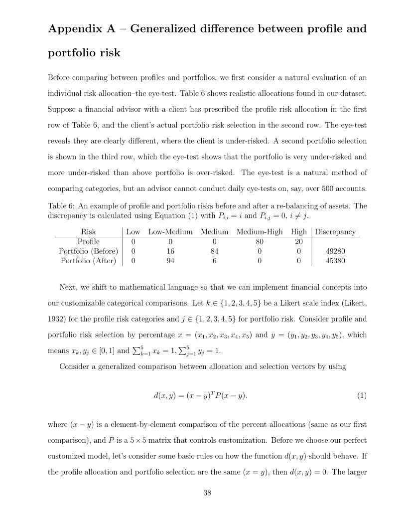
Before comparing between profiles and portfolios, we first consider a natural evaluation of an
individual risk allocation–the eye-test. Table 6 shows realistic allocations found in our dataset.
Suppose a financial advisor with a client has prescribed the profile risk allocation in the first
row of Table 6, and the client’s actual portfolio risk selection in the second row. The eye-test
reveals they are clearly different, where the client is under-risked. A second portfolio selection
is shown in the third row, which the eye-test shows that the portfolio is very under-risked and
more under-risked than above portfolio is over-risked. The eye-test is a natural method of
comparing categories, but an advisor cannot conduct daily eye-tests on, say, over 500 accounts.
Table 6: An example of profile and portfolio risks before and after a re-balancing of assets. Thediscrepancy is calculated using Equation (1) with Pi,i = i and Pi,j = 0, i 6= j.
Risk Low Low-Medium Medium Medium-High High DiscrepancyProfile 0 0 0 80 20
Portfolio (Before) 0 16 84 0 0 49280Portfolio (After) 0 94 6 0 0 45380
Next, we shift to mathematical language so that we can implement financial concepts into
our customizable categorical comparisons. Let k ∈ {1, 2, 3, 4, 5} be a Likert scale index (Likert,
1932) for the profile risk categories and j ∈ {1, 2, 3, 4, 5} for portfolio risk. Consider profile and
portfolio risk selection by percentage x = (x1, x2, x3, x4, x5) and y = (y1, y2, y3, y4, y5), which
means xk, yj ∈ [0, 1] and∑5
k=1 xk = 1,∑5
j=1 yj = 1.
Consider a generalized comparison between allocation and selection vectors by using
d(x, y) = (x− y)TP (x− y). (1)
where (x− y) is a element-by-element comparison of the percent allocations (same as our first
comparison), and P is a 5×5 matrix that controls customization. Before we choose our perfect
customized model, let’s consider some basic rules on how the function d(x, y) should behave. If
the profile allocation and portfolio selection are the same (x = y), then d(x, y) = 0. The larger
38

the comparison, the more different the allocation and selection of risk are.
If we view allocations and selections as points in Euclidean space, it most natural to compute
discrepancy via the now Euclidean metric in 1, where P is now a positive definite matrix. Some
of the issues of this approach are as follows:
• If P is the identity matrix given as
P :=
1 0 0 0 0
0 1 0 0 0
0 0 1 0 0
0 0 0 1 0
0 0 0 0 1
.
then d(x, y) is now a sum of the squared deviation between each risk category. The two
portfolio selections of 100% low and 100% low-medium, are equidistant from the profile
allocation in Table 6. This is clearly unreasonable from a financial perspective, as the
difference is much larger than for the 100% low allocation than the 100% low-medium
allocation.
• If P is a diagonal matrix we can alleviate the problem indicated above. For example,
setting Pi,i = i gives
P :=
1 0 0 0 0
0 2 0 0 0
0 0 3 0 0
0 0 0 4 0
0 0 0 0 5
.
where d(x, y) =∑5
i=1 i(xi − yi)2 heavily penalizes discrepancies in higher risk categories.
This ensures that the distance between 100% high and 100% low-medium is twice as
large as that between 100% low and 100% low-medium. Unfortunately, this approach
39

introduces new complexities that we discovered when applying it to our data. The client
in Table 6 made a trade on particular date, that clearly moved them further from their
profile allocation. According to the metric, however, the trade moved them closer, which
is clearly unreasonable.
• The previous two matrices have only zeros as off diagonal terms and therefore the dis-
crepancy that uses the those matrices only compare the same categories. Consider the
penalization matrix that penalizes off diagonal terms given by
P :=
1 0 0 0 1
0 1 0 0 0
0 0 1 0 0
0 0 0 1 0
0 0 0 0 1
.
which yields d(x, y) =∑5
i=1(xi − yi)2 + (x1 − y1) ∗ (x5 − y5) The new term in the sum–a
penalization of misallocations in the low category has been added, but only if there is
also a misallocation in the high category (and vice versa). As it turns out, off-diagonal
terms place a heavier penalty on not just if there is a misallocation, but how they are
misallocated. This comparison will show us that not all misallocations are equal. A
penalization matrix that penalizes how far the misallocations are from the stated goals is
P :=
0 1 2 3 4
1 0 1 2 3
2 1 0 1 2
3 2 1 0 1
4 3 2 1 0
.
Notice that the diagonal terms are zero, which works in this configuration since we are
considering all misallocations in the off-diagonal terms. We could also relax the as-
sumption that the penalization matrix is symmetric, and allow for higher penalties for
40

over-risked profiles. A penalization matrix where we penalize an over-risked profile more
than under-risked could be
P :=
0 1 2 3 4
1 0 1 2 3
1 1 0 1 2
1 1 1 0 1
1 1 1 1 0
.
Consider another perspective that views profile and portfolio risk allocations and selections
as discrete probability distributions. It is most natural to compute discrepancy via an infor-
mation theoretic divergence such as Kullback-Liebler (K-L) divergence (Kullback and Leibler,
1951). Unfortunately this approach also leads to non-useful results. For example, consider a
profile of 100% low-medium, and two portfolio selections of 100% low and 100% high give the
same K-L divergence with the same sign, where we lose magnitude of the difference and whether
the portfolio is under- or over-risked. Other divergences were explored, but these suffered from
the same problems as the K-L divergences.
These metrics and divergences are designed to directly compare risk categories to evaluate
profile and portfolio risk alignment. The advantage of the proposed metric is that they can be
customized to calculate profile and portfolio risk alignment. We introduced equal and unequal
successive weightings for each category to inject ordering of the categories, and allow for the
natural conceptualization of risk to be included in the calculation. However, there are ever-
present problems with each calculation method that ruin the overall interpretations of results
across a dealership. In conclusion, we suggest the financial concept of value-at-risk is a much
more feasible method to compare profile risk allocations and portfolio risk selections.
41

Appendix B - Value-at-Risk methodology
Consider x be the profile risk allocation. Let µ denote the mean return vector and Σ be the
covariance matrix of the representative risk category ETFs. The α-level VaR on a KYC risk
profile is given by
VaRα(x) = xTµ+√xTΣx · zα ,
where zα is an appropriate α-quantile from a standard normal distribution. In this report,
we let α = 0.01. We have chosen five iShares ETFs with µ = [0.52, 1.97, 2.21, 2.93, 4.23],
σ = [0.13, 5.53, 6.48, 9.68, 15.22], and
ρ =
1 −0.22 −0.16 −0.23 0.07
−0.22 1 0.79 0.59 0.12
−0.16 0.79 1 0.78 0.31
−0.23 0.59 0.78 1 0.06
0.07 0.12 0.31 0.06 1
which yield
Σ = σTρσ =
0.016900 −0.158158 −0.134784 −0.289432 0.138502
−0.158158 30.580900 28.309176 31.582936 10.099992
−0.134784 28.309176 41.990400 48.926592 30.573936
−0.289432 31.582936 48.926592 93.702400 8.839776
0.138502 10.099992 30.573936 8.839776 231.648400
Appendix C - Distribution of VaRs across KYC informa-
tion
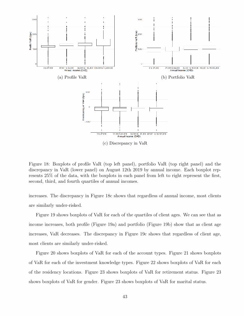
Next, we investigate a series of boxplots for the variables in Table 1. Figure 18 shows boxplots
of VaR at for each of the income levels quartiles. We can see that as income increases, both
profile (Figure 18a) and portfolio (Figure 18b) show that as annual income increases, VaR
42
(a) Profile VaR (b) Portfolio VaR
(c) Discrepancy in VaR
Figure 18: Boxplots of profile VaR (top left panel), portfolio VaR (top right panel) and thediscrepancy in VaR (lower panel) on August 12th 2019 by annual income. Each boxplot rep-resents 25% of the data, with the boxplots in each panel from left to right represent the first,second, third, and fourth quartiles of annual incomes.
increases. The discrepancy in Figure 18c shows that regardless of annual income, most clients
are similarly under-risked.
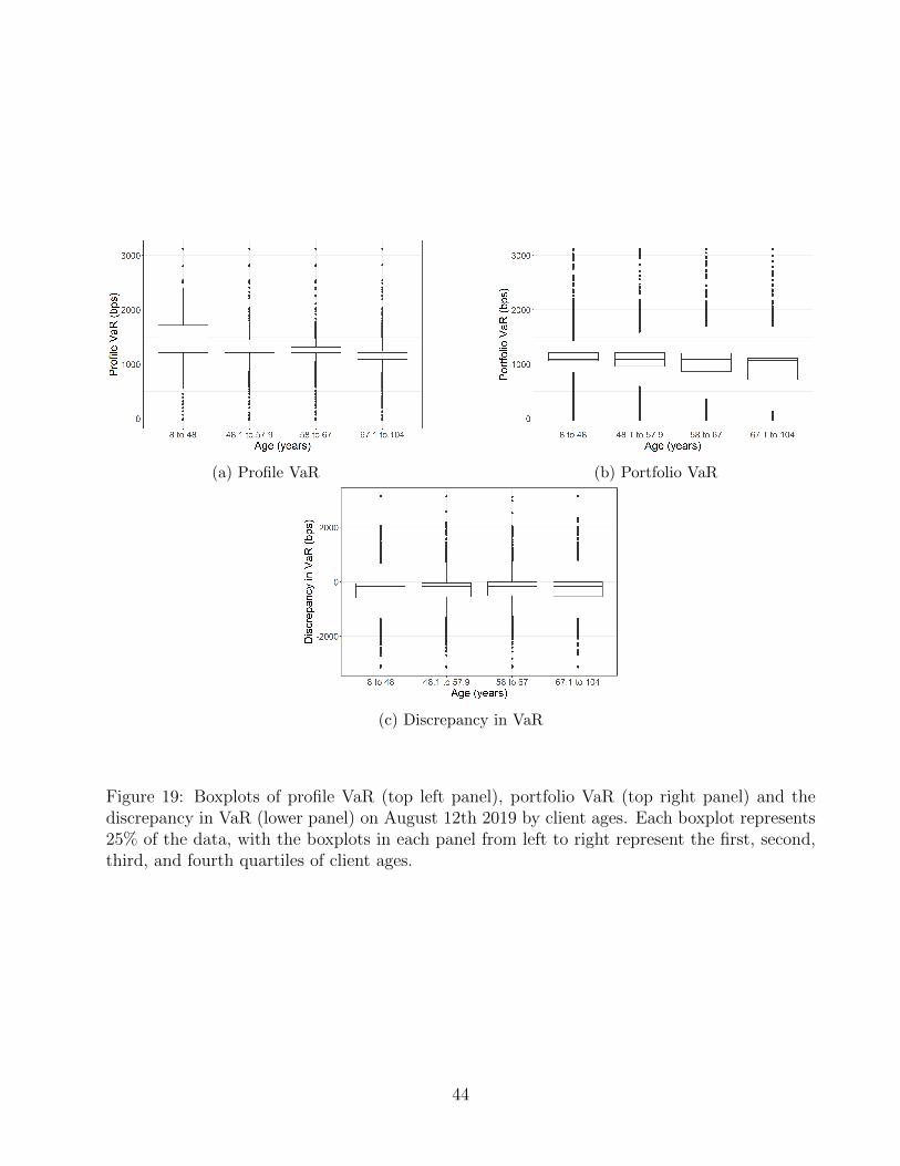
Figure 19 shows boxplots of VaR for each of the quartiles of client ages. We can see that as
income increases, both profile (Figure 19a) and portfolio (Figure 19b) show that as client age
increases, VaR decreases. The discrepancy in Figure 19c shows that regardless of client age,
most clients are similarly under-risked.
Figure 20 shows boxplots of VaR for each of the account types. Figure 21 shows boxplots
of VaR for each of the investment knowledge types. Figure 22 shows boxplots of VaR for each
of the residency locations. Figure 23 shows boxplots of VaR for retirement status. Figure 23
shows boxplots of VaR for gender. Figure 23 shows boxplots of VaR for marital status.
43
(a) Profile VaR (b) Portfolio VaR
(c) Discrepancy in VaR
Figure 19: Boxplots of profile VaR (top left panel), portfolio VaR (top right panel) and thediscrepancy in VaR (lower panel) on August 12th 2019 by client ages. Each boxplot represents25% of the data, with the boxplots in each panel from left to right represent the first, second,third, and fourth quartiles of client ages.
44

(a) Profile VaR (b) Portfolio VaR
(c) Discrepancy in VaR
Figure 20: Boxplots of profile VaR (top left panel), portfolio VaR (top right panel) and thediscrepancy in VaR (lower panel) on August 12th 2019 by account type.
45

(a) Profile VaR (b) Portfolio VaR
(c) Discrepancy in VaR
Figure 21: Boxplots of profile VaR (top left panel), portfolio VaR (top right panel) and thediscrepancy in VaR (lower panel) on August 12th 2019 by investment knowledge.
46

(a) Profile VaR (b) Portfolio VaR
(c) Discrepancy in VaR
Figure 22: Boxplots of profile VaR (top left panel), portfolio VaR (top right panel) and thediscrepancy in VaR (lower panel) on August 12th 2019 by residency location.
47

(a) Profile VaR (b) Portfolio VaR
(c) Discrepancy in VaR
Figure 23: Boxplots of profile VaR (top left panel), portfolio VaR (top right panel) and thediscrepancy in VaR (lower panel) on August 12th 2019 by retirement status.
48

(a) Profile VaR (b) Portfolio VaR
(c) Discrepancy in VaR
Figure 24: Boxplots of profile VaR (top left panel), portfolio VaR (top right panel) and thediscrepancy in VaR (lower panel) on August 12th 2019 by gender.
49

(a) Profile VaR (b) Portfolio VaR
(c) Discrepancy in VaR
Figure 25: Boxplots of profile VaR (top left panel), portfolio VaR (top right panel) and thediscrepancy in VaR (lower panel) on August 12th 2019 by marital status.
50

(a) Annual income (b) Total market value
(c) Investment knowledge
Figure 26: Boxplots of age against annual income (top left panel), total portfolio market value(top right panel), and investment knowledge (lower panel).
Since age is related to the accumulation of experience and wealth, we consider the distri-
bution of ages against annual income, market value, and investment knowledge in Figure 26.
Figure 26a show a comparison of age and income quartiles. Similarly, Figure 26b shows age and
total asset market value quartiles. Figure 26c shows age and investment knowledge quartiles.
51