measuring equity: a survey of indices for public...
TRANSCRIPT
MEASURING EQUITY 1
Measuring Equity: A Survey of Indices for Public Administration1
Shu Wang, PhD Student
University of Illinois at Chicago
Sharon H. Mastracci, Associate Professor
University of Illinois at Chicago
1 Prepared for presentation at the Public Values Research Consortium conference, June 3-5, 2012, Chicago, Illinois. DRAFT: Please do not cite—this is an early version of an ongoing project.
MEASURING EQUITY 2
Measuring Equity: A Survey of Indices for Public Administration
Abstract
As the third pillar of public administration, social equity has been relatively underexplored compared to efficiency and effectiveness, with the lack of measurement as a significant obstacle. Equity is fundamental to public administration as a public value toward which public administrators should direct their efforts. We rely on the definition of equity put forth by Rawls in A Theory of Justice and applied to public administration by Frederickson, and focus on equitable distribution of service delivery rather than equitable access to services. We then survey five widely-used equity measurement gauges, examine the strengths and weaknesses of each, and conclude that the Theil statistic and Blau index are very useful to public administration researchers to capture multiple-group comparisons of equity. An important contribution of this paper is to demonstrate the potential measurability of an inherently subjective construct like equity.
As the third pillar of public administration, social equity has been underexplored, with
the lack of measurement as a significant obstacle. Besides normative advocate for incorporating
social equity into public administration practice, little empirical studies have been conducted to
evaluate to what extent this value has been realized. As Chitwood (1974) points out, there is
ambiguity when public administrators are deciding the specified characteristics of a service
whose magnitude determines the amount of service to be delivered. There are also administrative
difficulties of assessing the extent to which potential recipients of service possess the specified
characteristic. Further, unequal treatment is often needed to bring the disadvantaged to the
average level in order to achieve an equitable outcome. Measurement of equity becomes critical
to determine the degree of inequality between groups, as well as how much an unequal treatment
is needed to bring the disadvantaged to a level ground.
This paper is intended to demonstrate the measurability of social equity as a public value
by introducing a few indicators that can be used to evaluate to what extent a policy realizes the
value of equity. Social equity is defined by Rawls’ theory of justice and Frederickson’s (1990)
compound theory in this paper. We propose a few measures to be applied to public
MEASURING EQUITY 3
administration, particularly for inequity of service delivery by reviewing key inequality measures
that have been used in social science research and discussing their strengths, weaknesses and
relevance to public administration research. Equality measures can be applied to capture
disproportionate distributions of services delivered by demographic category of recipients, or by
geographic location/political entity. Acknowledging the complexity of social equity issues in the
context of growing disparity between the haves and have-nots, we believe that any equity
measure should be applicable to more than just race/ethnicity categories. Race and ethnicity are
increasingly insufficient as proxies for socioeconomic status. The best gauge of equity identifies
the disadvantaged by unmet needs for resources and services, rather than race/ethnic categories.
Therefore, our recommendations for the measures are based on their flexibility for
accommodating multiple groups, reflecting our belief in the multidimensionality of the concept
of “the disadvantaged.” We also suggest spatial analysis as a useful tool for illustrating inequity
of geographical distribution. The section below contains the definitions of equity including
foundational definitions by John Rawls (1974), and the corresponding interpretation in public
administration by H. George Frederickson (1990). The following section includes a brief analysis
of five equity measures found in public administration and fields that inform public
administration, as well as an application of two indices to illustrate their use. We then briefly
discuss spatial analysis, and then conclude with a summary of our assessments of the five indices,
as well as thoughts on further research.
Defining Equity
We need to ground our examination of various equity measures in a specific definition of
equity, which is an inherently subjective construct. We begin with equity as defined by Rawls,
MEASURING EQUITY 4
who, according to Hart (1974), provides the theoretical framework for public administration.
Equity according to Frederickson (1990) is discussed next, followed by an analysis of affirmative
action as an example of remedial inequality.
Rawlsian Equity. It is important to construct a clear definition of equity for public
administration to advance the body of knowledge in the field and to provide clearer and more
coherent guidelines to practitioners. After decades of scholarship and practice that focused on
promoting the values of efficiency and effectiveness, Frederickson (1971) accurately pointed out
that public administration should not only be concerned about efficiency, but also about
efficiency for whom. Frederickson established equity as the “third pillar of public administration”
(1980, p. 37) in what he called The New Public Administration. John Rawls’ theory of justice
thus provides a solid philosophical foundation for the value of social equity in public
administration. Differing from Deutsch’s (1975) equity that states that the gain of each individual
in a society should be based upon their potential productivity, Rawlsian justice pays attention to
the welfare of the minority and the disadvantaged, and expresses the belief quoted below that
echoes the equity value that New Public Administration advocates hold (Rawls, 1974, p. 3-4):
Justice denies that the loss of freedom for some is made right by the greater good shared by others. It does not allow that the sacrifices imposed on a few are outweighed by the larger sum of advantages enjoyed by many.
In detail, there are three key components of Rawlsian justice theory. First, the original
position as a philosophical position ensures an arena of moral discourse where all individuals
make decisions behind “the veil of ignorance” without knowing their historical heritage and
social status. The veil of ignorance enables society to reach an agreement that is the most
beneficial for the least advantaged, because each individual may be in an unfavorable position.
MEASURING EQUITY 5
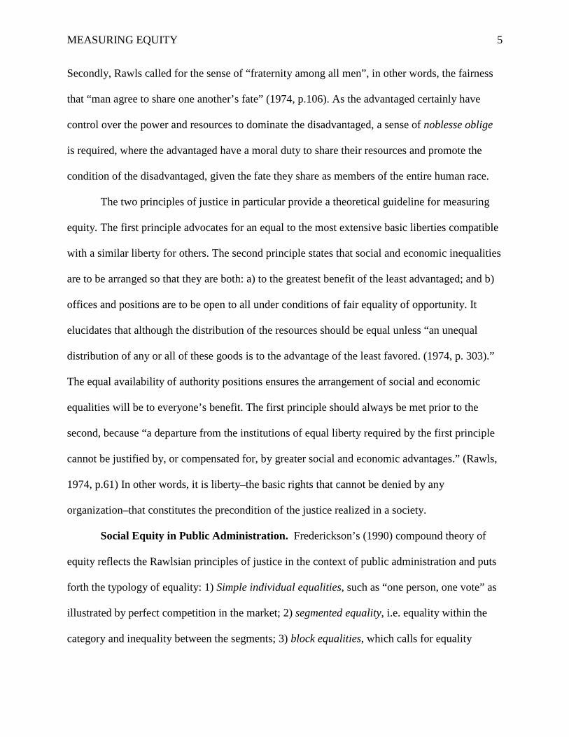
Secondly, Rawls called for the sense of “fraternity among all men”, in other words, the fairness
that “man agree to share one another’s fate” (1974, p.106). As the advantaged certainly have
control over the power and resources to dominate the disadvantaged, a sense of noblesse oblige
is required, where the advantaged have a moral duty to share their resources and promote the
condition of the disadvantaged, given the fate they share as members of the entire human race.
The two principles of justice in particular provide a theoretical guideline for measuring
equity. The first principle advocates for an equal to the most extensive basic liberties compatible
with a similar liberty for others. The second principle states that social and economic inequalities
are to be arranged so that they are both: a) to the greatest benefit of the least advantaged; and b)
offices and positions are to be open to all under conditions of fair equality of opportunity. It
elucidates that although the distribution of the resources should be equal unless “an unequal
distribution of any or all of these goods is to the advantage of the least favored. (1974, p. 303).”
The equal availability of authority positions ensures the arrangement of social and economic
equalities will be to everyone’s benefit. The first principle should always be met prior to the
second, because “a departure from the institutions of equal liberty required by the first principle
cannot be justified by, or compensated for, by greater social and economic advantages.” (Rawls,
1974, p.61) In other words, it is liberty–the basic rights that cannot be denied by any
organization–that constitutes the precondition of the justice realized in a society.
Social Equity in Public Administration. Frederickson’s (1990) compound theory of
equity reflects the Rawlsian principles of justice in the context of public administration and puts
forth the typology of equality: 1) Simple individual equalities, such as “one person, one vote” as
illustrated by perfect competition in the market; 2) segmented equality, i.e. equality within the
category and inequality between the segments; 3) block equalities, which calls for equality
MEASURING EQUITY 6
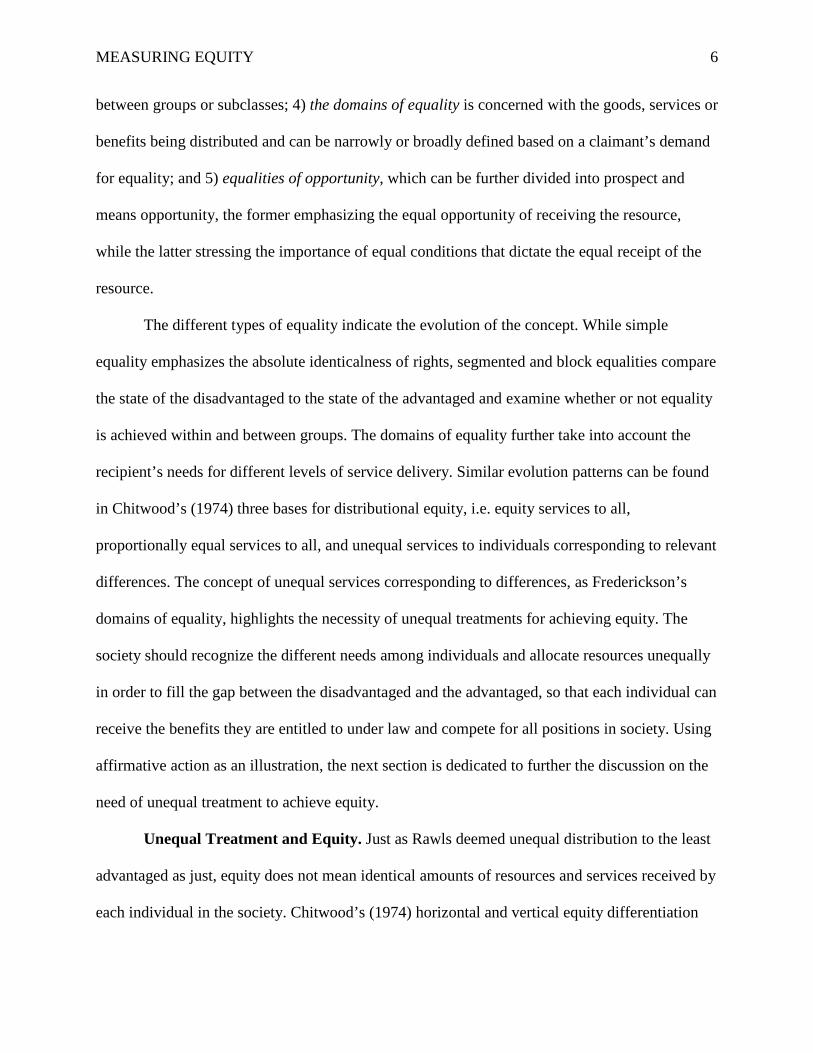
between groups or subclasses; 4) the domains of equality is concerned with the goods, services or
benefits being distributed and can be narrowly or broadly defined based on a claimant’s demand
for equality; and 5) equalities of opportunity, which can be further divided into prospect and
means opportunity, the former emphasizing the equal opportunity of receiving the resource,
while the latter stressing the importance of equal conditions that dictate the equal receipt of the
resource.
The different types of equality indicate the evolution of the concept. While simple
equality emphasizes the absolute identicalness of rights, segmented and block equalities compare
the state of the disadvantaged to the state of the advantaged and examine whether or not equality
is achieved within and between groups. The domains of equality further take into account the
recipient’s needs for different levels of service delivery. Similar evolution patterns can be found
in Chitwood’s (1974) three bases for distributional equity, i.e. equity services to all,
proportionally equal services to all, and unequal services to individuals corresponding to relevant
differences. The concept of unequal services corresponding to differences, as Frederickson’s
domains of equality, highlights the necessity of unequal treatments for achieving equity. The
society should recognize the different needs among individuals and allocate resources unequally
in order to fill the gap between the disadvantaged and the advantaged, so that each individual can
receive the benefits they are entitled to under law and compete for all positions in society. Using
affirmative action as an illustration, the next section is dedicated to further the discussion on the
need of unequal treatment to achieve equity.
Unequal Treatment and Equity. Just as Rawls deemed unequal distribution to the least
advantaged as just, equity does not mean identical amounts of resources and services received by
each individual in the society. Chitwood’s (1974) horizontal and vertical equity differentiation
MEASURING EQUITY 7
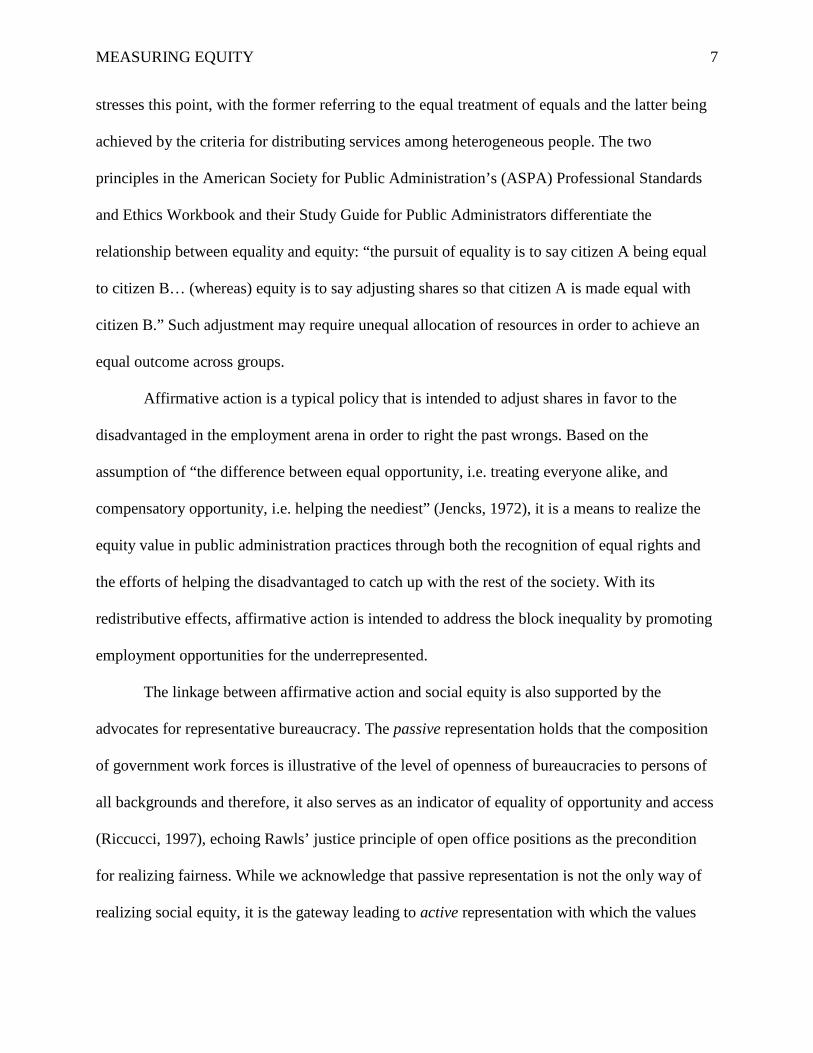
stresses this point, with the former referring to the equal treatment of equals and the latter being
achieved by the criteria for distributing services among heterogeneous people. The two
principles in the American Society for Public Administration’s (ASPA) Professional Standards
and Ethics Workbook and their Study Guide for Public Administrators differentiate the
relationship between equality and equity: “the pursuit of equality is to say citizen A being equal
to citizen B… (whereas) equity is to say adjusting shares so that citizen A is made equal with
citizen B.” Such adjustment may require unequal allocation of resources in order to achieve an
equal outcome across groups.
Affirmative action is a typical policy that is intended to adjust shares in favor to the
disadvantaged in the employment arena in order to right the past wrongs. Based on the
assumption of “the difference between equal opportunity, i.e. treating everyone alike, and
compensatory opportunity, i.e. helping the neediest” (Jencks, 1972), it is a means to realize the
equity value in public administration practices through both the recognition of equal rights and
the efforts of helping the disadvantaged to catch up with the rest of the society. With its
redistributive effects, affirmative action is intended to address the block inequality by promoting
employment opportunities for the underrepresented.
The linkage between affirmative action and social equity is also supported by the
advocates for representative bureaucracy. The passive representation holds that the composition
of government work forces is illustrative of the level of openness of bureaucracies to persons of
all backgrounds and therefore, it also serves as an indicator of equality of opportunity and access
(Riccucci, 1997), echoing Rawls’ justice principle of open office positions as the precondition
for realizing fairness. While we acknowledge that passive representation is not the only way of
realizing social equity, it is the gateway leading to active representation with which the values
MEASURING EQUITY 8
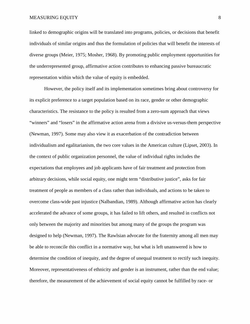
linked to demographic origins will be translated into programs, policies, or decisions that benefit
individuals of similar origins and thus the formulation of policies that will benefit the interests of
diverse groups (Meier, 1975; Mosher, 1968). By promoting public employment opportunities for
the underrepresented group, affirmative action contributes to enhancing passive bureaucratic
representation within which the value of equity is embedded.
However, the policy itself and its implementation sometimes bring about controversy for
its explicit preference to a target population based on its race, gender or other demographic
characteristics. The resistance to the policy is resulted from a zero-sum approach that views
“winners” and “losers” in the affirmative action arena from a divisive us-versus-them perspective
(Newman, 1997). Some may also view it as exacerbation of the contradiction between
individualism and egalitarianism, the two core values in the American culture (Lipset, 2003). In
the context of public organization personnel, the value of individual rights includes the
expectations that employees and job applicants have of fair treatment and protection from
arbitrary decisions, while social equity, one might term “distributive justice”, asks for fair
treatment of people as members of a class rather than individuals, and actions to be taken to
overcome class-wide past injustice (Nalbandian, 1989). Although affirmative action has clearly
accelerated the advance of some groups, it has failed to lift others, and resulted in conflicts not
only between the majority and minorities but among many of the groups the program was
designed to help (Newman, 1997). The Rawlsian advocate for the fraternity among all men may
be able to reconcile this conflict in a normative way, but what is left unanswered is how to
determine the condition of inequity, and the degree of unequal treatment to rectify such inequity.
Moreover, representativeness of ethnicity and gender is an instrument, rather than the end value;
therefore, the measurement of the achievement of social equity cannot be fulfilled by race- or
MEASURING EQUITY 9
gender-counting, but can only be done through the examination of resources, services and
opportunities across groups. In the next section, we reviewed several key inequality measures
used in social sciences and evaluated their strengths and limitations. We propose that these
measures can be applied to evaluating unequal distribution of resources and services and
quantifying how “far off” the resources received by the disadvantaged is from the average level.
As such, we can take a step further in social equity research from advocating what should be
done to gauging how much should be done.
Inequality Measures: Strengths and Limitations
This section includes a brief analysis of five equity measures found in public
administration, as well as an application of two indices to illustrate their use.
Multidimensionality of the disadvantaged. Before discussing how to measure
inequality between two groups (i.e. the advantaged and the disadvantaged), it is important to note
that the disadvantaged is a multidimensional concept that should not only be labeled by race or
gender, but also take into account the people’s social origin and life experience that lead up to
the less fortunate position, such as education, parents’ occupation, household income, etc. The
implementation of affirmative action sometimes becomes problematic when solely relying on
demographic characteristics as the indicator for potential beneficiaries. Affirmative action
captures the centrality and singularity of race or gender, and creates increasing polarization of
African American and White, and male and female at the same time (Newman, 1997). As
Frederickson notes (2005, p. 34):
The terrain of social equity has shifted from more-or-less exclusive concentration on the equity issues of minorities to broad consideration of how to achieve social equity in the context of growing disparity between the haves and have-nots, recognizing that minorities constitute a disproportionate percentage of the have-nots.
MEASURING EQUITY 10
Labeling a group as the disadvantaged simply by its race or gender fails to fully capture
their unmet need while overlooking the adversity faced by other races. Better measurement is
needed to better identify the people who truly suffer from a disadvantaged situation that needs
preferential policies to help them reach a level playing field. Therefore, the measures we discuss
below are focused on inequality between two groups; rather than dividing individuals by their
race or gender, many examples shown below are governments or countries with unequal
economic status. These examples illustrate a broader scope of recipient equity and the relevance
of inequality measures to public administration research.
Review of inequality measures. In this section, we discuss the strengths and limitations
of several commonly-used measures of inequality in public administration, and in fields that
inform public administration.2
2 Providing proofs of the mathematical properties of these indices is beyond the scope of this paper. See the appendices in Reardon and Firebaugh (2002) for such information.
One aspect of these indices that we characterize as a limitation
may not necessarily be a limitation, depending upon the object under study and the application of
the inequality measure. That aspect is the ability to measure inequality across more than two
groups. Many inequality measures gauge disparities dichotomously: Men compared to women,
urban versus rural, white versus non-white, and etcetera. In order to capture the
multidimensionality of the disadvantaged, we compared multichotomous measures favorably to
their dichotomous counterparts, due to the greater flexibility of the former over the latter, as
multigroup measures are still applicable in a two-group setting. Furthermore, multigroup
comparisons are often more applicable in social science research, as Reardon and Firebaugh
observe (2002, p. 34): “As U.S. society becomes more racially diverse, two-group measures of
segregation will become increasingly inadequate for describing complex patterns of racial
segregation and integration.” Other strengths and weaknesses are determined as such according
MEASURING EQUITY 11
to their appropriateness of use by social science researchers. Five indices are discussed, roughly
in order of their development chronologically, with growing degrees of complexity and
applicability: The Gini Coefficient, the Duncan Index of Dissimilarity, the Herfindahl-
Hirschman Index, the Blau Index, and the Theil Statistic.
The Gini Coefficient. First published in 1912, the Gini coefficient is perhaps the earliest
of the inequality measures found in the social science literature that have also found their way to
public administration. It captures the distance between equal income distribution across a
population and the actual income distribution across the population. It ranges from zero,
denoting income parity, to one, denoting complete income inequality across a population.
Among OECD countries, the United States’ current Gini coefficient before taxes and transfers is
0.486; indicating less inequality than Italy (0.534) and the UK (0.506), but more income
inequality than Japan (0.462), Canada (0.441), Norway (0.410), and Korea (0.344) (OECD,
2012). The Gini gauges income distribution by country (although other geographic
configurations are possible as well), which is illustrated by the area between the line of parity
and the Lorenz curve, as shown in the figure below.
MEASURING EQUITY 12
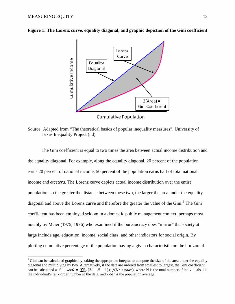
Figure 1: The Lorenz curve, equality diagonal, and graphic depiction of the Gini coefficient
Source: Adapted from “The theoretical basics of popular inequality measures”, University of Texas Inequality Project (nd)
The Gini coefficient is equal to two times the area between actual income distribution and
the equality diagonal. For example, along the equality diagonal, 20 percent of the population
earns 20 percent of national income, 50 percent of the population earns half of total national
income and etcetera. The Lorenz curve depicts actual income distribution over the entire
population, so the greater the distance between these two, the larger the area under the equality
diagonal and above the Lorenz curve and therefore the greater the value of the Gini.3
3 Gini can be calculated graphically, taking the appropriate integral to compute the size of the area under the equality diagonal and multiplying by two. Alternatively, if the data are ordered from smallest to largest, the Gini coefficient can be calculated as follows:𝐺 = ∑ (2𝑖 − 𝑁 − 1)𝑥𝑖 /(𝑁2 ∗ 𝑥𝑏𝑎𝑟)𝑁
𝑖=1 , where N is the total number of individuals, i is the individual’s rank order number in the data, and x-bar is the population average.
The Gini
coefficient has been employed seldom in a domestic public management context, perhaps most
notably by Meier (1975, 1976) who examined if the bureaucracy does “mirror” the society at
large include age, education, income, social class, and other indicators for social origin. By
plotting cumulative percentage of the population having a given characteristic on the horizontal
MEASURING EQUITY 13
axis and the cumulative percentage of civil servants with the same characteristic on the vertical
axis, Meier (1975, 1976) graphically showed inequality of bureaucrats’ representation with the
Gini coefficient indicating how a group with a given characteristic is (un)equally distributed
across bureaucracy in relation to its percentage in the population. Although Meier’s work does
not directly address social equity, it sheds light on the Gini coefficient can be applied to a
broader context beyond income distribution, but any resource or service distribution (e.g. civil
servants) across population.
One limitation of the Gini coefficient is that it only measures distributions of income; it
does not allow the researcher to conclude that equal distributions imply economic welfare. For
instance, over most of the 20th century, India and Sweden had similar Gini coefficients but while
the relatively equal income distribution in Sweden indicated overall welfare, but in India, the low
Gini coefficient simply captured the fact that people were all similarly poor. A second limitation
is that Gini focuses only on income, and does not capture wealth disparities. Income is defined as
wages and salaries from paid labor or proprietorship, whereas wealth includes relatively illiquid
assets like real property and investments. A disparity in wealth, for instance home ownership,
across race and ethnic groups would not be captured by the Gini coefficient. An implication of
this limitation is that Gini probably understates inequality where general welfare includes wage
and salary income as well as assets.
Duncan Dissimilarity Index. The dissimilarity index has been used for decades to
capture disparate outcomes between two groups in a wide range of policy areas, including
occupational segregation by race and gender (Albelda, 1985, 1986; Beller, 1985; Bertaux, 1991;
Bielby & Baron, 1986; Blau & Hendricks, 1979; Deutsch, Fluckinger & Silber, 1994; Fuchs,
1975; King, 1992; Madden, 1977; Watts, 1995), residential segregation and migration patterns
MEASURING EQUITY 14
(Duncan & Duncan, 1956; Fietosa, et al 2007; Holloway & Wright, 2012; Morello-Frosch, 2006;
White, Kim & Glick, 2005; Wong, 2002), school desegregation (Frankel, 2011), even health
disparities by race and residential location (Skinner et al, 2003). Its most common application,
however, has been to determine the presence of occupational segregation by race or gender,
which is how it has been applied in public administration (Pitts, 2005; Rocha & Hawkes, 2009;
Sneed, 2007). Occupational segregation by race or gender, sometimes referred to as glass walls
or barriers to moving across occupations in contrast to glass ceilings, which represent barriers to
advancement, occupational segregation is one type of inequality in employment, and
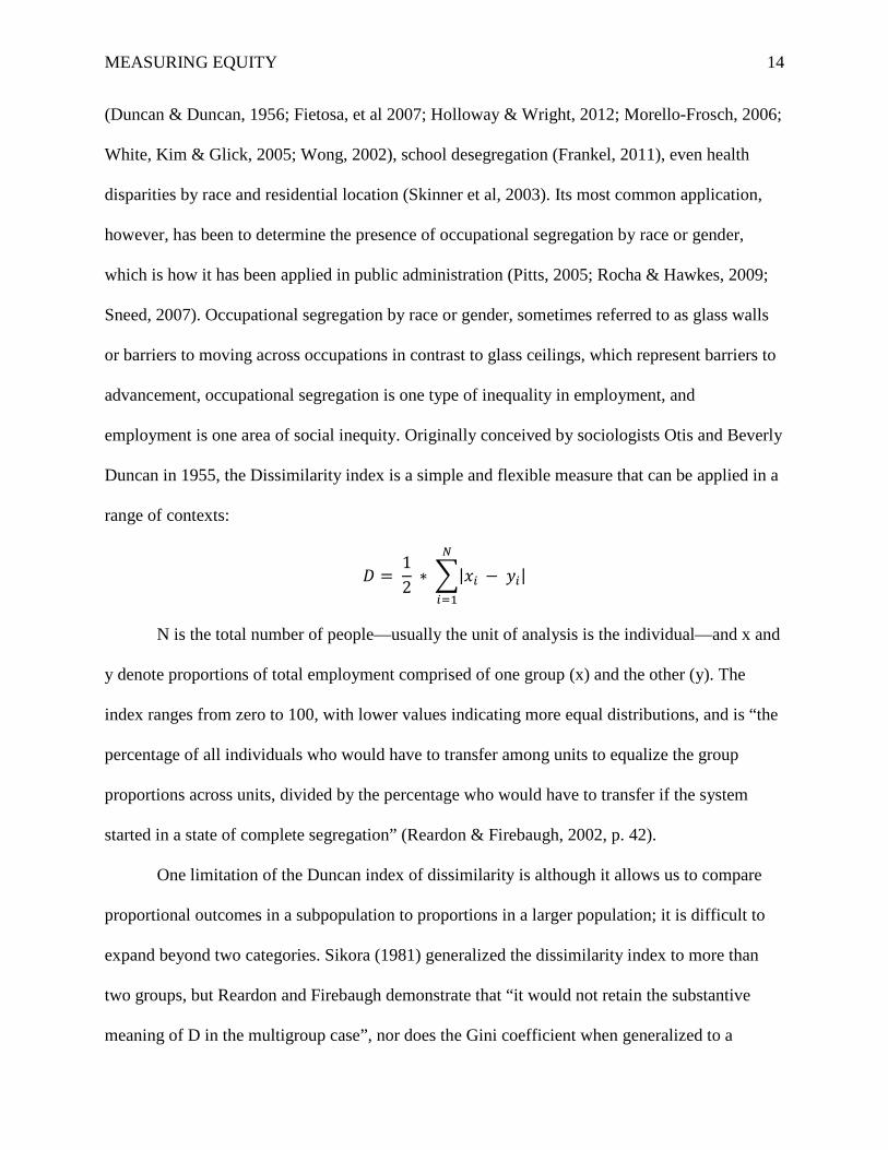
employment is one area of social inequity. Originally conceived by sociologists Otis and Beverly
Duncan in 1955, the Dissimilarity index is a simple and flexible measure that can be applied in a
range of contexts:
𝐷 = 12
∗ �|𝑥𝑖 − 𝑦𝑖|𝑁
𝑖=1
N is the total number of people—usually the unit of analysis is the individual—and x and
y denote proportions of total employment comprised of one group (x) and the other (y). The
index ranges from zero to 100, with lower values indicating more equal distributions, and is “the
percentage of all individuals who would have to transfer among units to equalize the group
proportions across units, divided by the percentage who would have to transfer if the system
started in a state of complete segregation” (Reardon & Firebaugh, 2002, p. 42).
One limitation of the Duncan index of dissimilarity is although it allows us to compare
proportional outcomes in a subpopulation to proportions in a larger population; it is difficult to
expand beyond two categories. Sikora (1981) generalized the dissimilarity index to more than
two groups, but Reardon and Firebaugh demonstrate that “it would not retain the substantive
meaning of D in the multigroup case”, nor does the Gini coefficient when generalized to a
MEASURING EQUITY 15
multigroup setting (2002, p. 49). What is more, in the multiple group case Duncan’s D “remains
constant in the case of exchanges that move individuals that move between units where the
groups are either over- or underrepresented in both” groups (Reardon & Firebaugh, 2002, p. 51).
When individuals are moved across groups, the index of dissimilarity should not remain constant.
This is a flaw in the Duncan Dissimilarity Index when attempting to apply it to a multiple-
category setting.
The Herfindahl Index. Like other inequality measures, The Herfindahl-Hirschman
Index (HHI) evolved from another discipline; in this case, from the Simpson index used in
ecology to gauge species diversity in a given ecosystem. HHI was developed in economics in the
1940s and 1950s to gauge concentration of market power across firms in an industry (Herfindahl,
1950; Hirschman, 1945). It has found a place in public administration by scholars studying the
distribution of resources, for instance, across school districts (Martin & Smith, 2005; Meier &
Bohte, 2003). Somewhat more commonly, HHI has been used in international contexts to study
budget allocations across political jurisdictions, including the United Kingdom (Andrews, Boyne,
Meier & O’Toole, 2005; Andrews & Boyne, 2006), Norway (Sorensen, 2007), The Netherlands
(Dijkgraaf & Gradus, 2007), and in OECD countries (Pina & Torres, 2003). HHI is used to
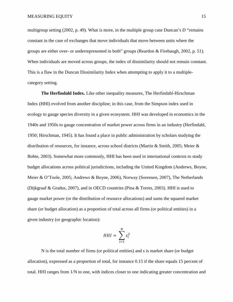
gauge market power (or the distribution of resource allocations) and sums the squared market
share (or budget allocation) as a proportion of total across all firms (or political entities) in a
given industry (or geographic location):
𝐻𝐻𝐼 = �𝑠𝑖2𝑁
𝑖=1
N is the total number of firms (or political entities) and s is market share (or budget
allocation), expressed as a proportion of total, for instance 0.15 if the share equals 15 percent of
total. HHI ranges from 1/N to one, with indices closer to one indicating greater concentration and
MEASURING EQUITY 16
more unequal distribution.
An important limitation to this measure is that it is highly sensitive to the definition of
boundaries. In market power studies for instance, HHI will vary greatly depending upon how the
market is defined. If a narrow definition is used—comparing firms in a very specific industry
and/or geography—one might find high concentrations of market power. If industry and
geography are defined such that a firm is said to compete with firms across a wide range of
industries all around the world, that single firm would be found to have less market power than if
it were assumed to compete in a narrowly-defined industry and/or geographic area or political
entity.
The Blau Index. The Blau index (1977) is fundamentally the same as HHI in that it
summarizes squared shares across groups, but the Blau is applied to groups by demographic
characteristics rather than by the economic construct of a market. In this way, the Blau index
avoids the limitation of HHI by not relying on subjective boundaries like the market within
which individual firms compete, in favor of “nominal parameters” (Blau, 1977, p. 8) such as sex,
race, national origin, ethnicity, and marital status. These parameters are not entirely equivocal, of
course, but are commonly understood in a consistent way in most cultural contexts such that the
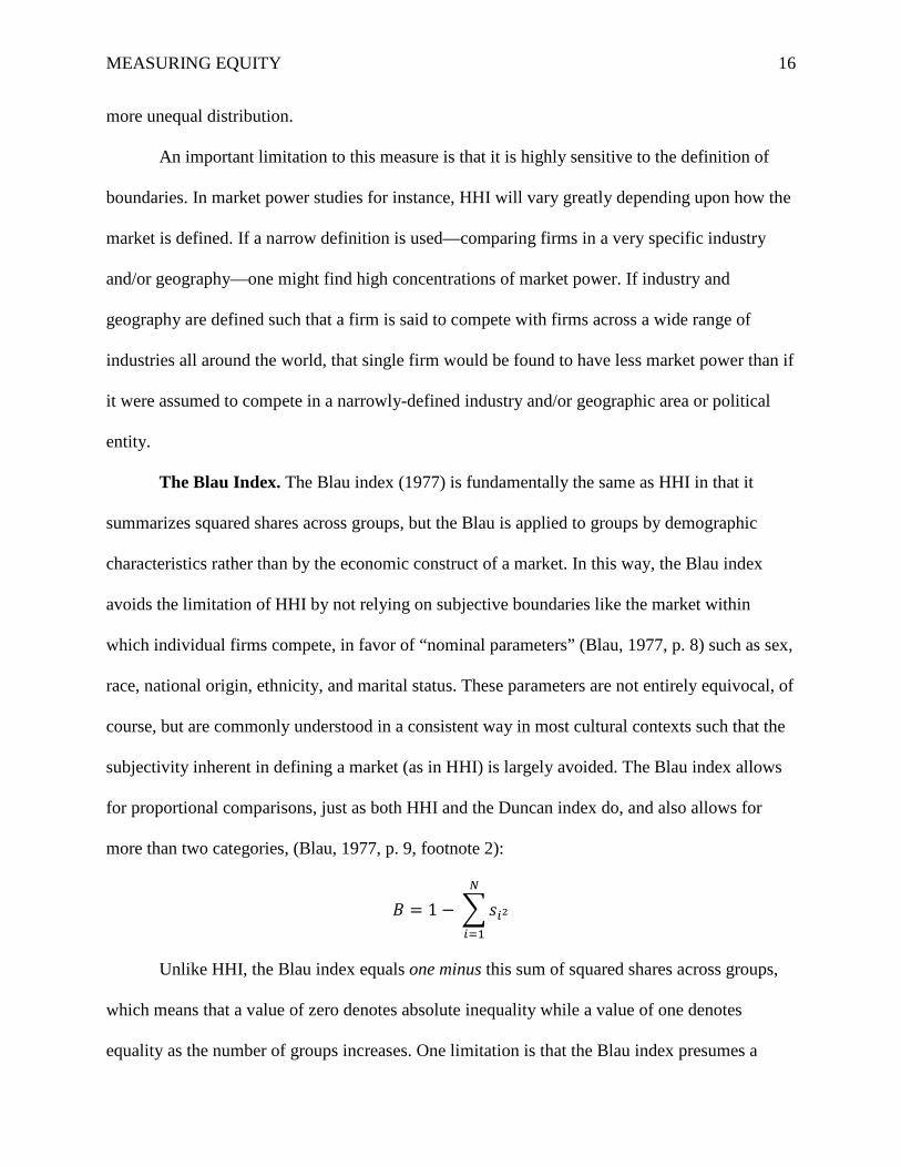
subjectivity inherent in defining a market (as in HHI) is largely avoided. The Blau index allows
for proportional comparisons, just as both HHI and the Duncan index do, and also allows for
more than two categories, (Blau, 1977, p. 9, footnote 2):
𝐵 = 1 − �𝑠𝑖2𝑁
𝑖=1
Unlike HHI, the Blau index equals one minus this sum of squared shares across groups,
which means that a value of zero denotes absolute inequality while a value of one denotes
equality as the number of groups increases. One limitation is that the Blau index presumes a

MEASURING EQUITY 17
particular definition of equity: Simple equal shares or unequal shares for unequal blocks or ranks.
That is, the Blau index suffers the same limitation as the Gini coefficient. Proper interpretation of
the Blau requires context: “When a few people are very rich and most are equally poor …
inequality is more pronounced than when wealth or power is more equally distributed … To say
that such extreme concentration of wealth or power means little inequality would be contrary to
common sense” (Blau, 1977, p. 9, emphasis supplied). In other words, the value resulting from
calculating a Blau index cannot be interpreted without knowledge of the distribution of income,
budget allocations, or whatever may be the outcome of interest.
The Theil Statistic. The Theil statistic evolved from an index in computer science to
measure information redundancy (Shannon & Weaver, 1949) to an income inequality measure in
economics (Theil, 1972). A standardized Theil statistic equal to zero indicates absolute parity of
income distribution, while one indicates absolute inequality:
𝑇 = 1𝑁
∗ � ∗𝑁
𝑖=1
�𝑥𝑖
𝑥𝑏𝑎𝑟 ∗ ln
𝑥𝑖𝑥𝑏𝑎𝑟
�
N is the total number of people (or groups), x-bar is average income, and xi is the income
of person “i” (or group “i”). The Theil statistic is the sum of the ratio of each person’s (or
group’s) income to average income multiplied by the natural log of that ratio. Multiplying this
sum by one over N standardizes it to the population (UTIP, nd). The maximum value of a non-
standardized Theil is equal to the natural log of N, so if the measure is not standardized, its
maximum value depends upon the size of the population.
A feature of this inequality measure, which is unique to the Theil statistic, is that not
only can it accommodate more than two groups; it can be decomposed to capture between-group
inequality, or Frederickson’s block inequality. In addition, the Theil statistic is not influenced by
otherwise innocuous transfers of units across groups, which is a problem with the Duncan index
MEASURING EQUITY 18
(Reardon & Firebaugh, 2002). Furthermore, its data requirements are less stringent than are the
data needs of other measures: Theil can be calculated using group averages, “For most practical
data, data that has some degree of aggregation or an underlying hierarchy (e.g. cities within
regions within nations), Theil’s T statistic is often a more appropriate and theoretically sound
tool” (UTIP, nd, para. 15).
Anything that can be divided into groups can be measured for inequality, and both overall
inequality can be captured as can comparisons between groups by decomposing Theil to a
between-group measure: “If members of a population can be classified into mutually exclusive
and completely exhaustive groups (e.g.: demographic categories like Blau’s “normative
parameters”, industries, occupations, or geographic regions) then Theil’s T statistic is made up of
two components, the between-group element and the within-group element” (UTIP, nd, para. 16).
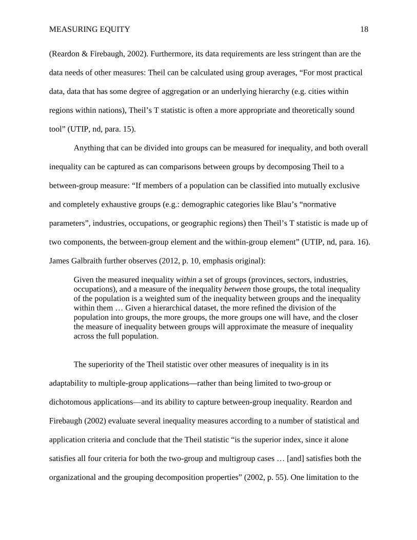
James Galbraith further observes (2012, p. 10, emphasis original):
Given the measured inequality within a set of groups (provinces, sectors, industries, occupations), and a measure of the inequality between those groups, the total inequality of the population is a weighted sum of the inequality between groups and the inequality within them … Given a hierarchical dataset, the more refined the division of the population into groups, the more groups, the more groups one will have, and the closer the measure of inequality between groups will approximate the measure of inequality across the full population.
The superiority of the Theil statistic over other measures of inequality is in its
adaptability to multiple-group applications—rather than being limited to two-group or
dichotomous applications—and its ability to capture between-group inequality. Reardon and
Firebaugh (2002) evaluate several inequality measures according to a number of statistical and
application criteria and conclude that the Theil statistic “is the superior index, since it alone
satisfies all four criteria for both the two-group and multigroup cases … [and] satisfies both the
organizational and the grouping decomposition properties” (2002, p. 55). One limitation to the
MEASURING EQUITY 19
use of the Theil statistic to gauge inequality arises not in its statistical properties, but in its
interpretation by researchers (UTIP, nd, para. 18):
A single Theil statistic is usually difficult to interpret, so whenever possible, it is advisable to have data over a number of time periods … Theil’s T statistic is very sensitive to the number of groups, so it is very difficult to compare measures across cross-sectional units. In other words, do not try to directly compare inequality across the 50 United States to inequality across the ten provinces of Canada. You can measure the inequality of many social and economic variables. Examples include the square footage of housing units, numbers of doctor visits, years of education and crop yields.
This cautionary note is similar to the one offered for the Gini coefficient. Just as low Gini
coefficients do not indicate high economic welfare across all contexts (recall the similarity of
Sweden and India discussed earlier), so must one take care not to compare Theil statistic across
incompatible groupings like U.S. states and Canadian provinces. Political boundary definitions
like municipalities, states, and provinces vary from country to country and are inherently
incomparable. Standardized categories, like per capita budget allocations or crop yields per acre,
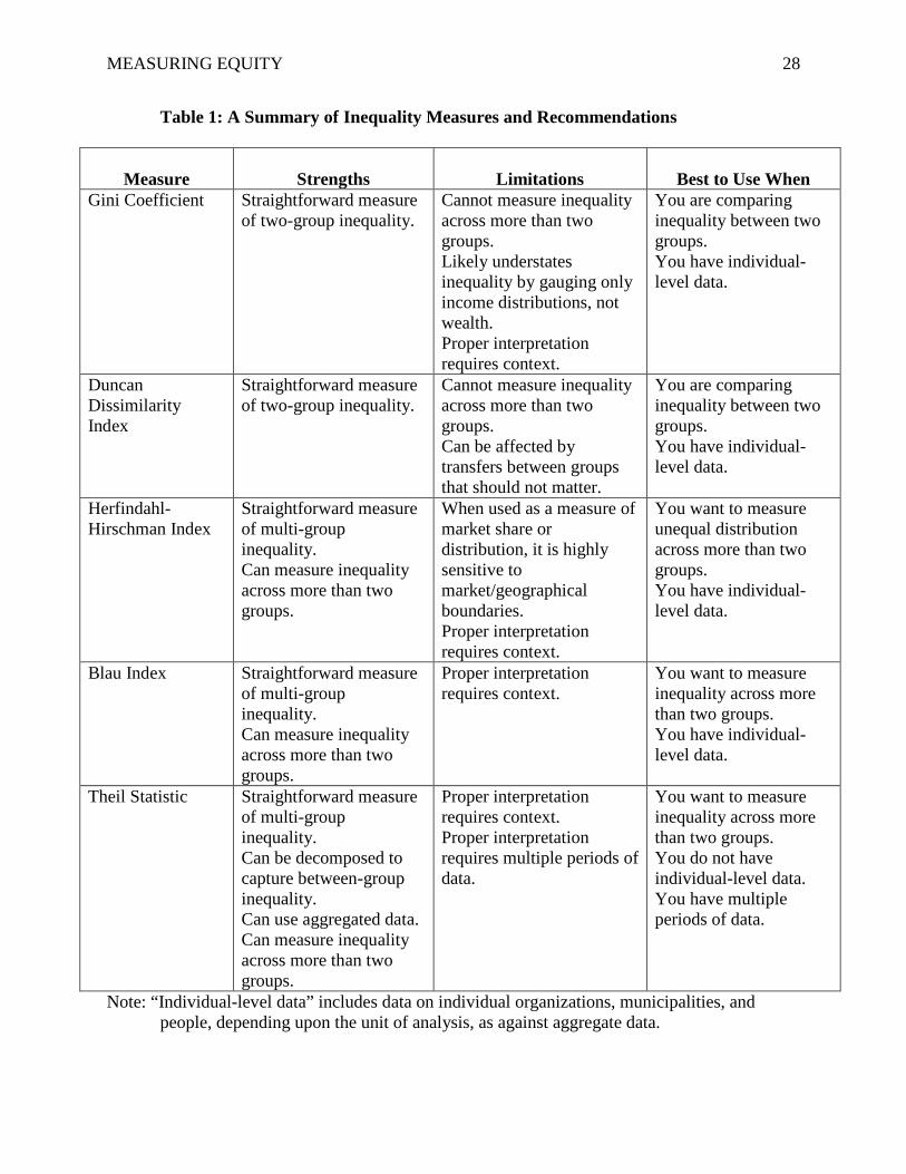
however, are comparable across contexts. Table 1 presents each measure’s strengths, limitations
and the scenarios in which they are of best use. In the next section we show the potential
contribution of these measures to public administration by discussing how to apply the Theil
statistic and Blau Index to analyzing equity of service delivery. These two indices are chosen as
examples for their flexibility to accommodate multiple groups and capture the
multidimensionality of the disadvantaged; as Table 1 presents, however, researchers are
encouraged to apply other indices to the scenarios that they deem fit.
Application of indices to gauge inequality by service delivery area. Efforts have been
made to measure equity in the service delivery area. For example, Lucy, Gilbert and Birkhead
(1977) categorized public services as routine, protective, developmental and social minimum
with respect to their functions. Routine services are the ones that are used on most days by most
MEASURING EQUITY 20
people, such as water supply, transit, and roads. Protective services help to maintain public order
by preventing the occurrence of undesirable events and providing a remedy when these events
occur, such as police, fire, courts, among others. Developmental services are aimed at the
physical, intellectual, and psychological potential of individual people; public education is a
good example for it. Social minimum services are the ones such as food stamps and public
housing that are targeted at the disadvantaged, an area commonly discussed of its redistribution
function. The authors then presented selected indicators of resources, activities, results and
opinions for each category. For example, expenditures for police patrol per 1,000 residents is an
indicator of resources, average police response time for activities, percent of crimes reported
cleared by neighborhood for output, and residents’ opinions about effectiveness and fairness for
impact. These indicators provide tools to quantify the input, process, output and impact of a type
of public service and evaluate equity of these measures.
Hird (1993) analyzed the equity implication of the nation’s hazardous waste cleanup
program, known as Superfund, by examining the geographic distribution of sites. Using a Tobit
regression model, the author predicted the likelihood of a site to be designated a Superfund site
with socioeconomic characteristics of the area in which the site located. Findings show that the
sites eligible for using Superfund and the likely beneficiaries of program expenditures live in
counties that are on average wealthier, better educated, and with lower rates of poverty. While
recognizing the symbolic appeal of the program for illustrating government’s responsibility for
negative externalities, the study concludes by pointing out the program’s failure to assign
sufficiently compensating liability or redistribute federal cleanup resources to the disadvantaged.
Rather, the tax revenue raised for Superfund is likely to be regressively redistributed to wealthier
communities.
MEASURING EQUITY 21
However, equal treatment at one stage often seems to mean unequal treatment at
subsequent stages, and that inequality of resources and activities are often required if equality of
impacts is the goal to be achieved (Lucy, et al, 1977). Although the indicators discussed provide
measures to compare input and output of service across populations, they do not answer the
question about how unequal the treatment should be in order to realize an equitable impact
distribution. Similarly, although Hird (1993) acknowledged the unequal exposure to
environmental risks across different groups and thus more resources may be needed for cleaning
up a site than others, he did not measure to what extent the risks and resources are inequitably
distributed.
To analyze such deviations from equality, a socioeconomic status index should be first
established to identify the basis on which the level of service distributed can be compared
between groups, whether they are defined by geographical areas, demographic characteristics or
income levels. Then, in addition to the proper measures for the service, it is important to develop
experiential measures (Lucy, et al, 1977) that are focused on the needs for public services that
vary by served population.
Both the Theil statistic and Blau index can be applied to analyze equity of service
delivery in public administration. Not only do the indices summarize how unequal is the
distribution between- and within-groups, but they also indicate to what extent remedial unequal
treatment is needed to fill in the gap. Related to service distribution, Lucy et al (1977) proposed a
three-test framework that mirrors the two Rawlsian principles: 1) equal treatment should be the
norm; 2) deviations from that norm should have specific justification, and 3) there should be a
minimum level (floor) for each service. With measures such as the Blau Index and Theil statistic,
MEASURING EQUITY 22
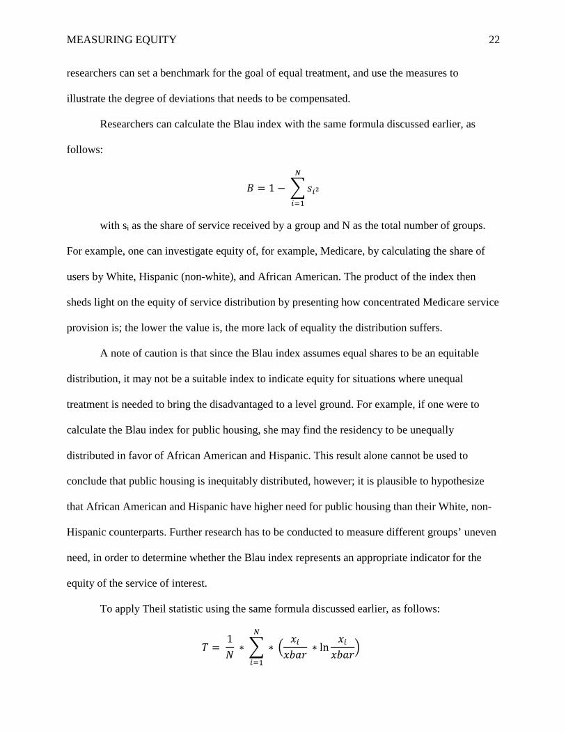
researchers can set a benchmark for the goal of equal treatment, and use the measures to
illustrate the degree of deviations that needs to be compensated.
Researchers can calculate the Blau index with the same formula discussed earlier, as
follows:
𝐵 = 1 − �𝑠𝑖2𝑁
𝑖=1
with si as the share of service received by a group and N as the total number of groups.
For example, one can investigate equity of, for example, Medicare, by calculating the share of
users by White, Hispanic (non-white), and African American. The product of the index then
sheds light on the equity of service distribution by presenting how concentrated Medicare service
provision is; the lower the value is, the more lack of equality the distribution suffers.
A note of caution is that since the Blau index assumes equal shares to be an equitable
distribution, it may not be a suitable index to indicate equity for situations where unequal
treatment is needed to bring the disadvantaged to a level ground. For example, if one were to
calculate the Blau index for public housing, she may find the residency to be unequally
distributed in favor of African American and Hispanic. This result alone cannot be used to
conclude that public housing is inequitably distributed, however; it is plausible to hypothesize
that African American and Hispanic have higher need for public housing than their White, non-
Hispanic counterparts. Further research has to be conducted to measure different groups’ uneven
need, in order to determine whether the Blau index represents an appropriate indicator for the
equity of the service of interest.
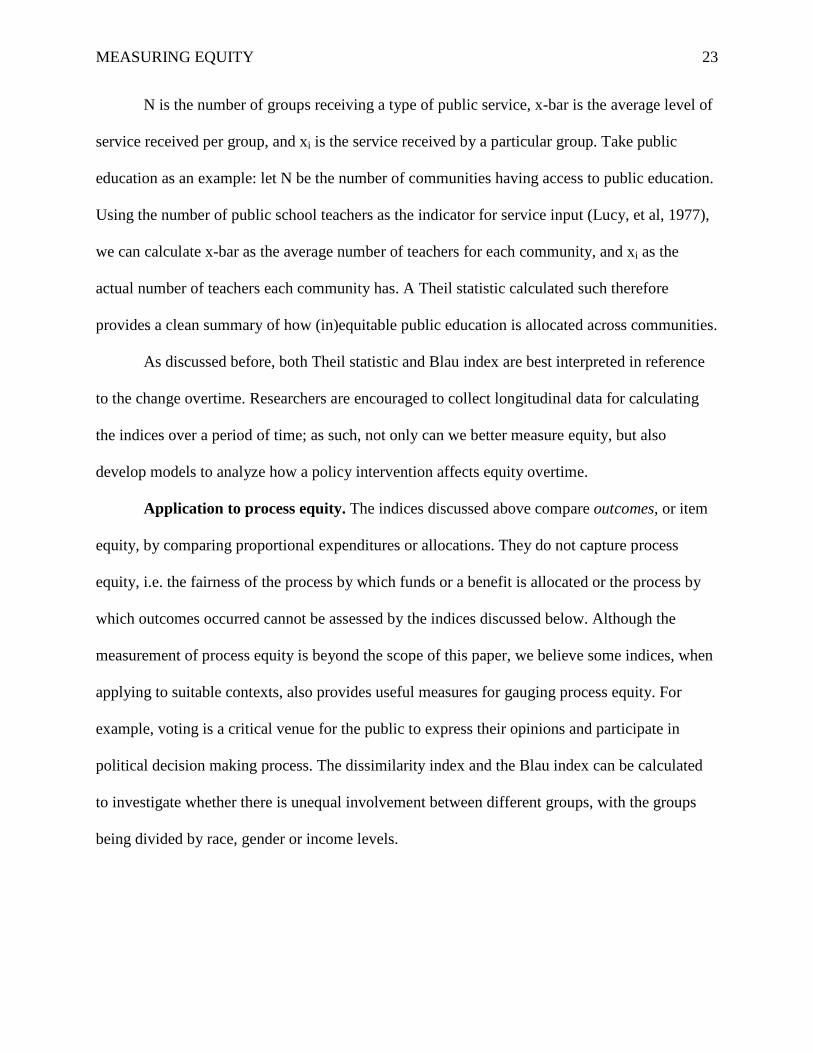
To apply Theil statistic using the same formula discussed earlier, as follows:
𝑇 = 1𝑁
∗ � ∗𝑁
𝑖=1
�𝑥𝑖
𝑥𝑏𝑎𝑟 ∗ ln
𝑥𝑖𝑥𝑏𝑎𝑟
�
MEASURING EQUITY 23
N is the number of groups receiving a type of public service, x-bar is the average level of
service received per group, and xi is the service received by a particular group. Take public
education as an example: let N be the number of communities having access to public education.
Using the number of public school teachers as the indicator for service input (Lucy, et al, 1977),
we can calculate x-bar as the average number of teachers for each community, and xi as the
actual number of teachers each community has. A Theil statistic calculated such therefore
provides a clean summary of how (in)equitable public education is allocated across communities.
As discussed before, both Theil statistic and Blau index are best interpreted in reference
to the change overtime. Researchers are encouraged to collect longitudinal data for calculating
the indices over a period of time; as such, not only can we better measure equity, but also
develop models to analyze how a policy intervention affects equity overtime.
Application to process equity. The indices discussed above compare outcomes, or item
equity, by comparing proportional expenditures or allocations. They do not capture process
equity, i.e. the fairness of the process by which funds or a benefit is allocated or the process by
which outcomes occurred cannot be assessed by the indices discussed below. Although the
measurement of process equity is beyond the scope of this paper, we believe some indices, when
applying to suitable contexts, also provides useful measures for gauging process equity. For
example, voting is a critical venue for the public to express their opinions and participate in
political decision making process. The dissimilarity index and the Blau index can be calculated
to investigate whether there is unequal involvement between different groups, with the groups
being divided by race, gender or income levels.
MEASURING EQUITY 24
Spatial Analysis
None of these measures account for spatial dimensions of inequality. Item inequity
between geographical areas by itself is an important topic in redistributive politics; examining
the geographical distribution of public services, particularly the ones whose physical locations
have great impacts on the service outcomes (e.g. bus stops, cleanup sites for environmental
hazards, public housing), sheds light on the measurement of social equity by mapping out the
uneven concentration between groups and illustrating the lack of resources for the areas that need
them the most. Spatial analysis tools developed by the planning discipline are of great value for
furthering our field that focuses on the behavior of the disadvantaged, and the mismatch between
their needs and the resources. The following uses public transit, a routine public service that is
particularly important for the people with limited mobility, as an example to illustrate how the
field of planning examines the equity of service delivery.
Compared to the studies that label the disadvantaged group with its demographic
characteristics, job accessibility as the key issue for a household’s welfare provides a more
accurate measure of the need of the disadvantaged and more directly addresses the equity issue.
Various studies have found the importance of travel modes for job access and employment
outcomes, particularly for minority and socially disadvantaged groups (Dawkins & Sanchez,
2005; Kain, 1968). Two main approaches are used to measure job accessibility: the potential-
based approach that calculates the number of job opportunities available depending on given
travel costs, distance and time, and excess commuting which represents the difference between
observed and theoretical minimal commuting given real distributions of jobs and housing
(Handy, 1997). Different approaches are used based on the research purposes and depending on
the measurement, but what the studies commonly agree upon is, there is inequality of job
MEASURING EQUITY 25
accessibility between car owners and public transit riders. For example, Sanchez (1999)
conducted a study to compare the connection between public transit and employment in Portland,
Oregon and Atlanta, Georgia, and found the access to public transit a significant factor in
determining average rates of labor participation.
With a number of studies focus on the spatial mismatch between job opportunities and
the residency of potential workforce, Kawabata and Shen (2007) add value to the body of
knowledge by taking into account the temporal changes in job accessibility and commuting time
between cars and public transit. The study shows that from 1990 to 2000, job accessibility was
enhanced by the shorter commuting time for the travelers of both travel modes, but the
relationship is stronger for public transit. In other words, the improvement of public transit has
greater potential to promote job accessibility than that of automobile. The authors thus proposed
the improvement of public transit systems as an approach not only to narrow disparities of
employment growth between car owners and captive riders but also to enhance social equity in
the labor market.
The application of spatial analysis on public transit can be extended to studying other
public services. Just as job access is the need for public transit, the researcher can identify an
indicator of the need for a type of service (e.g. crime rates), an indicator for the resources and
service (number of police officers in the area), and analyze the mismatch between the two by
area to gain understanding of equitable service distribution geographically.
Conclusion and Next Steps
In this study, we set out to establish the importance of measuring inequality in the spirit
of furthering research in social equity as the third pillar of public administration. Five indices

MEASURING EQUITY 26
that have appeared in the public administration literature are reviewed for their strengths and
weaknesses and we conclude that although no single measure is without its flaws, two measures
prove particularly appealing. First, the ability to decompose the Theil statistic into within-group
and between-group inequality allows researchers to capture multiple dimensions of inequality
and potentially provide more nuanced recommendations to address it. The ability to use
aggregated data and the capacity for multigroup comparisons are features of this measure, while
the need for multiple periods of data is a shortcoming. Second, the Blau index’s ease of use
makes it appealing to researchers. The central concern with this index is the warning that
researchers must interpret their findings in context rather than to use results on face value, but
this is a useful bit of advice for any gauge in social science research. Unlike the Theil statistic, it
does not require multiple periods of data for comparison, but nor does it decompose into within-
and between-group inequality measures. Furthermore, individual-level data is needed.
Depending upon the research question and availability of data, these shortcomings may not be so
after all.
We then propose to apply the measures such as the Theil statistic and the Blau index to
service delivery area and examine how unequal a type of service is allocated across different
groups. The next step is to choose a suitable service delivery area and calculate the Theil statistic
for it as a demonstration for the equity measurement proposed here. A longitudinal dataset would
be most desirable for interpreting equity overtime and analyzing the impacts of the policies that
are intended to enhance social equity.
This paper contributes to social equity research by introducing inequality measures to
public administration to demonstrate the measurability of social equity. We do not, however,
suggest that the indices are the only measures for social equity. Rather, it is our hope that this
MEASURING EQUITY 27
paper will intrigue further discussion of measuring social equity and move forward the research
on this value. The fact that these measures are borrowed from other social science fields also
highlights the potential of interdisciplinary collaboration.
MEASURING EQUITY 28
Table 1: A Summary of Inequality Measures and Recommendations
Measure
Strengths
Limitations
Best to Use When
Gini Coefficient Straightforward measure of two-group inequality.
Cannot measure inequality across more than two groups. Likely understates inequality by gauging only income distributions, not wealth. Proper interpretation requires context.
You are comparing inequality between two groups. You have individual-level data.
Duncan Dissimilarity Index
Straightforward measure of two-group inequality.
Cannot measure inequality across more than two groups. Can be affected by transfers between groups that should not matter.
You are comparing inequality between two groups. You have individual-level data.
Herfindahl-Hirschman Index
Straightforward measure of multi-group inequality. Can measure inequality across more than two groups.
When used as a measure of market share or distribution, it is highly sensitive to market/geographical boundaries. Proper interpretation requires context.
You want to measure unequal distribution across more than two groups. You have individual-level data.
Blau Index Straightforward measure of multi-group inequality. Can measure inequality across more than two groups.
Proper interpretation requires context.
You want to measure inequality across more than two groups. You have individual-level data.
Theil Statistic Straightforward measure of multi-group inequality. Can be decomposed to capture between-group inequality. Can use aggregated data. Can measure inequality across more than two groups.
Proper interpretation requires context. Proper interpretation requires multiple periods of data.
You want to measure inequality across more than two groups. You do not have individual-level data. You have multiple periods of data.
Note: “Individual-level data” includes data on individual organizations, municipalities, and people, depending upon the unit of analysis, as against aggregate data.
MEASURING EQUITY 29
References
Albelda, R. (1986). Occupational segregation by race and gender, 1958 – 1981. Industrial and Labor Relations Review, 39, 404-411.
Albelda, R. (1985). Nice work if you can get it: Segmentation of white and black women workers in the postwar period. Review of Radical Political Economics, 17, 72-85.
Andrews, R., Boyne, G.A., Meier, K.J. & O’Toole, L. (2005). Representative bureaucracy, organizational strategy, and public service performance: An empirical analysis of English local government. Journal of Public Administration Research and Theory, 15, 489-504.
Andrews, R., Boyne, G.A. & Walker, R.M. (2006). Strategy content and organizational performance: An empirical analysis. Public Administration Review, 66, 52-63.
Beller, A.H. (1985). Changes in the sex composition of U.S. occupations, 1960-1981. Journal of Human Resources, 20, 235-249.
Bertaux, N.E. (1991). The roots of today’s ‘women’s jobs’ and ‘men’s jobs’: Using the index of dissimilarity to measure occupational segregation by gender. Explorations in Economic Theory, 28, 433-459.
Bielby, W. & Baron, J. (1986). Men and women at work: Sex segregation and statistical discrimination. American Journal of Sociology, 91, 759-799.
Blau, P.M. (1977). Inequality and heterogeneity: A primitive theory of social structure. New York, NY: The Free Press.
Blau, F.D. & Hendricks, W.E. (1979). Occupational segregation by sex: Trends and prospects. The Journal of Human Resources, 24, 197-210.
Chitwood, S.R. (1974). Social equity and social service productivity. Public Administration Review, 34, 29-35.
Dawkins, C. J., Shen, Q., & Sanchez, T. W. (2005). Race, space, and unemployment duration. Journal of Urban Economics, 58(1), 91-113.
Deutsch, J., Fluckinger, Y. & Silber, J. (1994). Measuring occupational segregation: Summary statistics and the impact of classification errors and aggregation. Journal of Econometrics, 61, 133-146.
Deutsch, M. (1975). Equity, equality, and need: What determines which value will be used as the basis of distributive justice? Journal of Social issues, 31(3), 137-149.
Dijkgraaf, E. & Gradus, R. (2007). Collusion in the Dutch waste collection market. Local Government Studies, 33, 573-588.
Duncan, O. D. & Duncan, B. (1955). A methodological analysis of segregation indexes. American Sociological Review, 20, 210-217.
Frederickson, H. G. (1971). Toward a new public administration. Toward a new public administration: The Minnowbrook perspective, 309-331.
Frederickson, H.G. (1990). Public administration and social equity. Public Administration Review, 50, 228-237.
Frederickson, H.G. (1996). Comparing the reinventing government movement with the New Public Administration. Public Administration Review, 56, 263-270.
Frederickson, H. G. (2005). Public administration and social equity. Public administration and law, 209.
Fuchs, V.R. (1975). A note on sex segregation in professional occupations. Explorations in Economic Research, 2, 105-111.
Handy, S. L., & Niemeier, D. A. (1997). Measuring accessibility: an exploration of issues and
MEASURING EQUITY 30
alternatives. Environment and planning A, 29, 1175-1194. Hart, D.K. (1974). Social equity, justice, and the equitable administrator. Public Administration
Review, 34, 3-11 Herfindahl, O.C. (1950). Concentration in the U.S. steel industry. New York, NY: Unpublished
doctoral dissertation, Columbia University. Hird, J. A. (1993). Environmental policy and equity: The case of Superfund. Journal of Policy
Analysis and Management, 12(2), 323-343. Hirschman, A.O. (1945) National power and the structure of foreign trade. Berkeley, CA:
University of California Press. Jencks, C. (1972). Inequality: A reassessment of the effect of family and schooling in America,
NY: Basic Books. Kain, J. F. (1968). Housing segregation, negro employment, and metropolitan decentralization.
The Quarterly Journal of Economics, 82(2), 175. Kawabata, M., & Shen, Q. (2007). Commuting inequality between cars and public transit: The
case of the San Francisco Bay Area, 1990-2000. Urban Studies, 44(9), 1759. King, M.C. (1992). Occupational segregation by race and sex, 1940-1988. Monthly Labor
Review, 115, 30-37. Lipset, S. M. (2003). The first new nation: The United States in historical and comparative
perspective: Transaction Pub. Lucy, W. H., Gilbert, D., & Birkhead, G. S. (1977). Equity in local service distribution. Public
administration review, 687-697. Madden, J.F. (1977). A spatial theory of sex discrimination. Journal of Regional Science, 17,
369-380. Martin, S. & Smith. P.C. (2005). Multiple public service performance indicators: Toward an
integrated statistical approach. Journal of Public Administration Research and Theory, 15, 599-613.
McGregor, E.B. (1974). Social equity and the public service. Public Administration Review, 34, 18-29.
Meier, K. J. (1975). Representative bureaucracy: An empirical analysis. The American Political Science Review, 69(2), 526-542.
Meier, K. J., & Nigro, L. G. (1976). Representative bureaucracy and policy preferences: A study in the attitudes of federal executives. Public administration review, 36(4), 458-469.
Meier, K.J. & Bohte, J. (2003). Span of control and public organizations: Implementing Luther Gulick’s research design. Public Administration Review, 63, 61-70.
Meier, K.J., Wrinkle, R.D. & Polinard, J.L. (1999). Representative bureaucracy and distributional equity: Addressing the hard question. Journal of Politics, 61, 1025-1039.
Mosher, F.C. (1968). Democracy and the Public Service. New York, NY: Oxford Press. Nalbandian, J. (1989). The US Supreme Court's" consensus" on affirmative action. Public
administration review, 38-45. Newman, M. A. (1997). Sex, race, and affirmative action: An uneasy alliance. Public
Productivity & Management Review, 295-307. Organisation for Economic Cooperation and Development (2012). Gini coefficient: Before taxes
and transfers. Material downloaded 5/12/12 from http://stats.oecd.org/Index.aspx?DataSetCode=INEQUALITY.
Pina, V. & Torres, L. (2003). Reshaping public sector accounting: An international comparative view. Canadian Journal of Administrative Sciences, 20, 334-350.
MEASURING EQUITY 31
Pitts, D.W. (2005). Diversity, representation, and performance: Evidence about race and ethnicity in public organizations. Journal of Public Administration Research and Theory, 15, 615-631.
Porter, D.O. & Porter, T.W. (1974). Social equity and fiscal federalism. Public Administration Review, 34, 36-43.
Rawls, J. (1974). A theory of justice. Cambridge, MA: Harvard University Press. Reardon, S.F. & Firebaugh, G. (2002). Measures of multigroup segregation. Sociological
Methodology, 32, 33-67. Riccucci, N. (2009). The pursuit of social equity in public administration: The road less traveled.
Public Administration Review, 69(3), 373-382. Rocha, R.R. & Hawkes, D.P. (2009). Racial diversity, representative bureaucracy, and equity in
multiracial school districts. Social Science Quarterly, 90, 326-344. Sanchez, T. W. (1999). The connection between public transit and employment. Journal of the
American Planning Association, 65(3), 284–296. Shannon, C.E. & Weaver, W. (1949). A mathematical theory of communication. Urbana, IL:
University of Illinois Press. Skinner, J.D., Weinstein, J.N., Sporer, S.M. & Wennberg, J.E. (2003). Racial, ethnic, and
geographic disparities in rates of knee arthroplasty among Medicare patients. New England Journal of Medicine, S49, 1350-1359.
Sneed, B.G. (2007). Glass walls in state bureaucracies: Examining the difference departmental function can make. Public Administration Review, 67, 880-891
Sorensen, R.J. (2007). Does dispersed public ownership impair efficiency? The case of refuse collection in Norway. Public Administration, 85, 1045-1058.
University of Texas Inequality Project. (nd). A nearly painless guide to computing Theil’s T Statistic. Material downloaded 5/8/12 from http://utip.gov.utexas.edu/tutorials.html.
University of Texas Inequality Project (nd). The theoretical basics of popular inequality measures. Material downloaded 5/8/12 from http://utip.gov.utexas.edu/tutorials.html.
Watts, M.J. (1995). Divergent trends in gender segregation by occupation in the USA: 1970–92. Journal of Post Keynesian Economics, 17, 357-379.
White, O. & Gates, B.L. (1974). Statistical theory and equity in the delivery of social services. Public Administration Review, 34, 43-51.