measuring discharge at a tradtitional small scale irrigation scheme; a personal report on the...

Page | 1

Personal Report on the Operation of the Traditional Irrigation Scheme Leza 1

February – July - November 2016 SMIS – SMALL SCALE & MICRO IRRIGATION SUPPORT PROJECT Bahir Dar, Amhara Region, Ethiopia

MEASURING DISCHARGE AT A TRADITIONAL SMALL SCALE IRRIGATION SCHEME

This report is a pilot study which researches the irrigation scheme of Leza 1.

One of the pilot irrigation schemes of SMIS project. The research focuses on how data is being collected in Ethiopia

when measuring the water discharge, and the possible different ways of measuring

discharge in irrigation schemes in Ethiopia. This is done by researching

traditional methods, and by trying to gain an impression of the efficiency of these

existing traditional measuring method in comparison with other possible

measurement tools and methods.

Executed by: Joy Jamilla Pengel Master student at Wageningen University:

International Land and Water Management

& Landscape Architecture

Special thanks to:

All the Colleagues of SMIS Amhara Abbay Basin Authority Bureau of Agriculture

District Agents (DA’s) of Leza 1 Farmers of the irrigation scheme Leza 1 Bureau of Water Resources in Bahir Dar Engineering Department, University of

Bahir Dar Koga (Durabilis) Farm

LIVES Project

Table of Contents Introduction ............................................................................................................................................ 1

Situation Description .......................................................................................................................... 1

SMIS Project ........................................................................................................................................ 1

Missing Knowledge ................................................................................................................................. 2

My Role ............................................................................................................................................... 2

Methodology Part 1 ................................................................................................................................ 3

Hypothesis............................................................................................................................................... 4

Results ..................................................................................................................................................... 5

Measurements .................................................................................................................................... 5

Total data combined ....................................................................................................................... 5

Data per Measuring Tool ................................................................................................................ 5

Data per point of measuring ........................................................................................................... 6

Data set in Graphs ........................................................................................................................... 9

Controlled flume channel in the hydraulics lab, University Bahir Dar .......................................... 11

Correction Factor and its Influence .................................................................................................. 11

Semi-Structured Interviews .............................................................................................................. 11

Observation ....................................................................................................................................... 15

Methodology 2 (Extra measurement work July 2016). ........................................................................ 19

Fieldwork ........................................................................................................................................... 20

The method we used in the field .................................................................................................. 20

Outcome Data Experiment 1 ........................................................................................................ 21

Possible Problems ......................................................................................................................... 21

Outcome Data Experiment 2 ........................................................................................................ 23

Conclusion ............................................................................................................................................. 25

Discussion and Reflection ................................................................................................................. 25

Recommendations ............................................................................................................................ 26

References ............................................................................................................................................ 28

Annex 1 .................................................................................................................................................... i

1.1 Methodology .................................................................................................................................. i

1.1.1 Methods used to calculate the water flow in the irrigation scheme ...................................... i

1.1.2 Interviews .............................................................................................................................. iv

1.1.3 Observations .......................................................................................................................... v

1.2 Data Sheet Current Meter ........................................................................................................... vi

1.3 Data sheet Floating Method ....................................................................................................... vii

Annex 2 ................................................................................................................................................ viii

Measurements taken on point 1: Main River .................................................................................. viii

Measurements taken on point 2: After first natural river ................................................................ xii

Measurements taken on point 3: After both natural rivers in the main channel ............................ xv

Measurements taken on point 4: Secondary channel ..................................................................... xvii

Measurements taken on point 5: More downstream of the main channel ................................... xviii

Measurements taken in the hydraulic laboratory at the Bahir Dar University .................................xx

Annex 3 ............................................................................................................................................... xxiii

EC Meter River Flow Measurement: Dilution-Gauging Methods ................................................... xxiii

Annex 4 .............................................................................................................................................. xxvii

Electric Conductivity (Dilution-Gauging) field Measurements taken near Bahir Dar Airport ........ xxvii

Electric Conductivity (Dilution-Gauging) field measurements taken at a stream called Infiranz on the road from Bahir Dar to Zege ................................................................................................... xxviii

Appendix 1 .......................................................................................................................................... xxix

List of contacts ................................................................................................................................ xxix

Page | 1

Figure 1: Children herding a cow

Introduction Situation Description Ethiopia is a federal democratic republic. In every region public institutions are mandated to manage the development, design, and construction of small scale irrigation schemes, and promote the quality use of micro irrigation technologies at the household level. The effectiveness of this work relies on well-resourced organizations that are led by skilled leaders and staffed with competent individuals.

The irrigation sector is the responsibility of a number of public and private organizations at all administrative levels. Development partners have responded to the GOE’s articulated priorities, and are providing significant support to the sector through large-scale programs and projects.

The region this report will be focused on is the Amhara Region, with an in-depth analysis of the scheme Leza 1 near Finote Selam. In this area there are usually 2 irrigation periods and 1 rain fed agriculture period creating 3 potential harvest times in a year. Nevertheless, this is not always feasible due to lack of rainfall or a late or early rain season. Also the amount of water available to the scheme during the two irrigation periods may not be sufficient, which means that certain farmers may not be able to irrigate their fields, or in the case that the water is being distributed equally to each farmer the amount of water is not enough for any of them. From interviews conducted during the study it seemed that when this phenomenon would occur the farmers usually decide to only irrigate the perennial crops. There are also many other issues which may occur inside an irrigation scheme, as there are numerous interventions to help and support the local farmers.

SMIS Project The SMIS project, in support of the SSI Capacity Building Strategy and the Household Irrigation Working Strategy, is designed to address specific aspects of organizational and technical capacity in relation to the work of SSI and MI. Together with other initiatives, programs and projects such as ATA, AGP-1, AGP-2 and LIVES, the SMIS project will support those public, and to a lesser extent, private institutions responsible for SSI and MI to become high performing organizations with staff that are ready to take on this challenge.

Page | 2

Figure 2: Pepper plant affected by lice in one of the farms in Leza 1

Missing Knowledge There has been quite some work done by SMIS, and its counterparts, to gather information on the pilot schemes. Henceforth to get a better understanding of how they are being managed, irrigated, the type of crops grown, etcetera. There is however still a limited understanding of the scheme water flow during the dry season. Additionally there is no knowledge as to how different measurements are being done.

My Role There are three different aspects I will focus on and which hopefully will start some discussion and additional research.

1. Trying to find out as much as possible on the Leza 1 irrigation scheme near Finote Selam. Calculating the amount of water that is available for the scheme. The type of crops grown. A rough calculation if the amount of water is enough for the crop production. Type of irrigation practised by the farmers. How the water is distributed. How decisions are being made if changes need to happen in the irrigation scheme. What are certain aspects that should be addressed and changed to ensure that

productivity of the farms increases? How is all this data being collected?

2. Using different measurement tools to measure the amount of water that flows into schemes, to gain a better understanding which measurement tools would work best in Ethiopia. Specifically to measure the traditional irrigation schemes. This is very important as one needs to gather that data before designing a modern irrigation scheme. What is the traditional method being used to identify the amount of water that

flows into the irrigation scheme? What are other methods that could be used to measure the amount of water that

goes into the irrigation scheme? Which one is more accurate?

3. Through my own observations and discussions with experts, I will try to identify certain aspects which in my own opinion need to be addressed to increase the production capacity of the farmers. What are the main problems that I encountered? What are possible solutions towards these obstacles?

Page | 3

Methodology Part 1 There are different types of methodology which are being used during this research to ensure that the data collected is as accurate as possible, as there are different objectives. To find out what is the most effective way to measure the discharge inside the irrigation channels of Ethiopia, different measurement methods will be used. The methods that we are going to use are the traditional floating method and a current meter. For the floating method we are using different materials to find out which is the most suitable. These materials will be: an orange, water bottle, wine bottle, and a leaf.

In addition to these research methods, interviews with the farmers (figure 3) and (traditional) water board members will take place to gain an even clearer understanding of the irrigation scheme we are looking into plus how the data collection usually takes place. To this our own observations will be added as this will give even better and more accurate information as to what is actually going on within the irrigation scheme; this may also guide the interviews. More details about the methodology is given in annex 1.

Figure 3: Farmers being interviewed during field visit

Page | 4

Hypothesis There are different outcomes that could occur during my research. The aim to find out as much as possible on the Leza 1 irrigation scheme near Finote Selam for instance does not have a clear picture yet as to what will be the outcome. Especially as every place is different and therefore the structure of the irrigation scheme is not so easily predicted except for its geographical aspects.

For the different measurement tools which are being used some hypothesis may be made. The floating method is the most commonly used method in Ethiopia. However, I expect that the methodology as to how they do the measurements is not very precise; the way that I have explained the methodology (see Annex 1) is probably not the way that it is done during fieldwork. I also predict that the current meter will be the most accurate method to calculate the amount of water in the scheme as the corrections of the method are most likely more accurate.

As for my own observations during the fieldwork about what are problems related to irrigation within the Leza 1 scheme I encounter, and solutions to certain problems: these are not aspects which I can already predict as I have not been to the irrigation scheme yet.

Figure 4: The corn/maize harvest

Page | 5

Results Measurements In this chapter you can find all the results gathered from the fieldwork. For the raw data and calculations of each discharge measurement see Annex 2.

Total data combined Table 1: Total Data Combined

Measurement point: Mean Depth (m)

Total Area (m2)

Mean Velocity (m/s)

Total Discharge (m3/s)

Point 1.1 Current meter 0.06 0.18 0.11 0.060 Point 1.2 Current meter 0.09 0.39 0.07 0.058 Point 1 Float Orange 0.169/0.1/0.06 Aver. 0.392 Aver. 0.28 0.109 Point 1 Float Bottle 0.169/0.1/0.06 Aver. 0.392 Aver. 0.26 0.101 Point 2 Float Orange 0.412/0.40 Aver. 2.220 Aver. 0.06 0.126 Point 2 Float Wine 0.412/0.40 Aver. 2.220 Aver.0.05 0.115 Point 2 Float Bottle 0.412/0.40 Aver. 2.220 Aver. 0.05 0.122 Point 3 Current meter 0.16 0.392 0.04 0.028 Point 3 Float Wine 0.184/0.16 Aver. 0.151 Aver. 0.13 0.019 Point 3 Float Orange 0.184/0.16 Aver. 0.151 Aver. 0.15 0.023 Point 3 Float Bottle 0.184/0.16 Aver. 0.151 Aver. 0.15 0.023 Point 3 Float Leaf 0.184/0.16 Aver. 0.151 Aver. 0.17 0.026 Point 4 Current meter 0.07 0.07 0.03 0.006 Point 5 Current meter 0.08 0.13 0.06 0.019 Point 5 Float Orange 0.084/0.08/0.07 Aver. 0.114 Aver. 0.22 0.025 Point 5 Float Bottle 0.084/0.08/0.07 Aver. 0.114 Aver. 0.24 0.028

Data per Measuring Tool Table 2: Data Current Meter


Total Area (m2)

Mean Velocity (m/s)


Point 1.1 Current meter 0.06 0.18 0.11 0.060 Point 1.2 Current meter 0.09 0.39 0.07 0.058 Point 3 Current meter 0.16 0.392 0.04 0.028 Point 4 Current meter 0.07 0.07 0.03 0.006 Point 5 Current meter 0.08 0.13 0.06 0.019

Table 3: Data Floating Method Orange


Total Area (m2)

Mean Velocity (m/s)


Point 1 Float Orange 0.169/0.1/0.06 Aver. 0.392 Aver. 0.28 0.109 Point 2 Float Orange 0.412/0.40 Aver. 2.220 Aver. 0.06 0.126 Point 3 Float Orange 0.184/0.16 Aver. 0.151 Aver. 0.15 0.023 Point 5 Float Orange 0.084/0.08/0.07 Aver. 0.114 Aver. 0.22 0.025

Page | 6

Table 4: Data Floating Method Water Bottle


Total Area (m2)

Mean Velocity (m/s)


Point 1 Float Bottle 0.169/0.1/0.06 Aver. 0.392 Aver. 0.26 0.101 Point 2 Float Bottle 0.412/0.40 Aver. 2.220 Aver. 0.05 0.122 Point 3 Float Bottle 0.184/0.16 Avter. 0.151 Aver. 0.15 0.023 Point 5 Float Bottle 0.084/0.08/0.07 Aver. 0.114 Aver. 0.24 0.028

Table 5: Data Floating Method Wine Bottle and Leaf


Total Area (m2)

Mean Velocity (m/s)


Point 2 Float Wine 0.412/0.40 Aver. 2.220 Aver.0.05 0.115 Point 3 Float Wine 0.184/0.16 Aver. 0.151 Aver. 0.13 0.019 Point 3 Float Leaf 0.184/0.16 Aver. 0.151 Aver. 0.17 0.026

Data per point of measuring Table 6: Point 1 Measurements Combined


Total Area (m2)

Mean Velocity (m/s)


Point 1.1 Current meter 0.06 0.18 0.11 0.060 Point 1.2 Current meter 0.09 0.39 0.07 0.058 Point 1 Float Orange 0.169/0.1/0.06 Aver. 0.392 Aver. 0.28 0.109 Point 1 Float Bottle 0.169/0.1/0.06 Aver. 0.392 Aver. 0.26 0.101

Figure 5: Photo of the site of point 1.

Figure 6: Photo of how the current meter measurements where conducted.

Notes: There were some waves in the water which might have affected the data. We couldn’t find a part of the river that was completely straight so that might also have influenced the data. Also with the current meter 1.1 the propeller was a bit out of the water while conducting the measurement; this may have caused some disturbance in results. However, when looking at the outcomes of both current meter tests they are nearly the same so the disturbance will probably have been minimal. It is interesting to see that the orange and bottle indicate a much lower velocity than the current meter.

Page | 7

Table 7: Point 2 Measurements Combined


Total Area (m2)

Mean Velocity (m/s)


Point 2 Float Orange 0.412/0.40 Aver. 2.220 Aver. 0.06 0.126 Point 2 Float Wine 0.412/0.40 Aver. 2.220 Aver.0.05 0.115 Point 2 Float Bottle 0.412/0.40 Aver. 2.220 Aver. 0.05 0.122



Total Area (m2)

Mean Velocity (m/s)


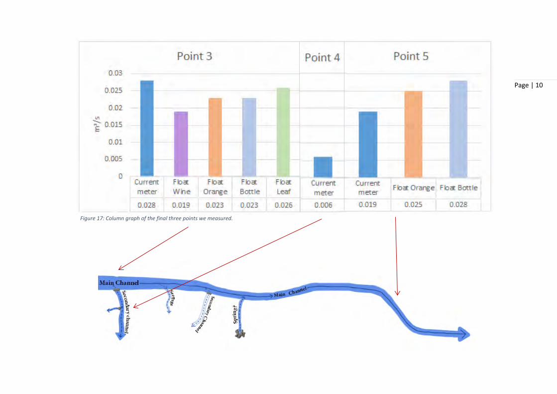
Point 3 Current meter 0.16 0.392 0.04 0.028 Point 3 Float Wine 0.184/0.16 Aver. 0.151 Aver. 0.13 0.019 Point 3 Float Orange 0.184/0.16 Aver. 0.151 Aver. 0.15 0.023 Point 3 Float Bottle 0.184/0.16 Aver. 0.151 Aver. 0.15 0.023 Point 3 Float Leaf 0.184/0.16 Aver. 0.151 Aver. 0.17 0.026

Figure 7: Photo point 2 when using a wine bottle for the floating method. Figure 8: Photo boy measuring the depth of the water.

Figure 9: Photo point 3 main channel downstream from the two natural rivers.

Figure 10: Photo of measurement being taken through current meter.

Notes: The boy moved a bit during the floating method this might have caused a bit of a disturbance. Also there was not enough flow to use the current meter. It is interesting to see that the wine bottle was faster than the orange and the water bottle as it was heavier and deeper in the water.

Notes: A lot of vegetation growing inside the channel and other floating materials. Also as you can see in the photos the water was carrying quite some sediment. With these measuring method the wine bottle again measured a much faster velocity than the other methods used.

Page | 8



Total Area (m2)

Mean Velocity (m/s)


Point 4 Current meter 0.07 0.07 0.03 0.006



Total Area (m2)

Mean Velocity (m/s)


Point 5 Current meter 0.08 0.13 0.06 0.019 Point 5 Float Orange 0.084/0.08/0.07 Aver. 0.114 Aver. 0.22 0.025 Point 5 Float Bottle 0.084/0.08/0.07 Aver. 0.114 Aver. 0.24 0.028

Figure 11: Photo point 4. Figure 12: Photo when using the current meter.

Figure 13: Photo of the vegetation growth in the secondary channel.

Figure 15: Photo of the use of the current meter. Figure 14: Photo point 5.

Notes: A lot of vegetation inside the channel. Because the farmer was actually not supposed to irrigate (there was no irrigation that day) we couldn’t test the floating method. The width of the intake was 19.5 cm and the depth of the water passing through was on average 9.2 cm

Notes: There was hardly any wind. More sediment in the water. Also there was quite some vegetation growth in the water. When we were doing the floating method we noticed that the bottle seemed to first always go to the right side and then bend back to the left, never exactly straight. The current meter measured quite a higher velocity than when using the floating method of the orange and the water bottle.

Page | 9

Data set in Graphs

Figure 16: Column graph showing all the data combined.

Page | 10

Figure 17: Column graph of the final three points we measured.

Page | 11

Controlled flume channel in the hydraulics lab, University Bahir Dar Table 11: table showing measurements done in the controlled flume channel

Measurement Tool: Mean Depth (m)

Total Area (m2)

Mean Velocity (m/s)


Current meter 0.27 0.04 0.05 0.012 Float Orange 0.27 0.081 Aver. 0.22 0.018 Float Water Bottle 0.27 0.081 Aver. 0.21 0.017 Float Wine Bottle 0.27 0.081 Aver. 0.22 0.018 Flume measurements 0.27 0.081 - 0.025

Figure 18: Photos of the flume channel used in the hydraulics laboratory of the University of Bahir Dar.

Correction Factor and its Influence Throughout this process there where different measurement systems used which of themselves had their own correction factors. The correction factor used for the floating method was 0.65. This was applied as this is the correction factor used in the traditional schemes in Ethiopia to ensure that the distortion of the measurement through the flow distribution across the channel, as show in Annex 1.1.1, can become as minimal as possible. For the current meter a correction factor or 0.10 was used.

Semi-Structured Interviews To gain a better understanding of the whole irrigation scheme of Leza 1 several interviews were conducted. With the farmers, DA of the scheme, and with the Woreda Agriculture Office. By talking to all these people it was possible to gain a picture of the scheme, how the scheme is being monitored and how it functions.

Notes: As it was inside there was no wind or other effects which could influence the data collected. There were some problems in the beginning as the measuring tool for the flume was not working. There was some dirt in the measuring tool which we first needed to clean up.

Another factor which might have influenced the outcome of the flume measurements is that the formula which was used to calculate the discharge inside the flume was incorrect. Usually you would just enter the level in an excel sheet which would then calculate the flow, or you would have a table of which you can read the answer. This wasn’t available for this flume. We used the formula given by the University of Bahir Dar.

Page | 12

1. What type of irrigation is being used? (furrow, wild flooding, sprinkler, drip, etc.?)

All people interviewed gave the same answer to this question. The main irrigation method being practiced in this scheme is furrow and wild flooding. There is also quite some water fetching (especially for the fields or home gardens where they cultivate for personal use). However, whether they actually do proper furrow irrigation remains questionable. Some of the fields that we visited where we looked at the type of irrigation used didn’t seem to be furrow irrigated areas even though the farmers claimed that they were using the furrow method for irrigation.

2. What is the amount of water that goes into the irrigation scheme?

There was no knowledge about the amount of water that goes into the irrigation scheme. The farmers have a fixed amount of time to irrigate their fields and then they have to close the secondary channel again. Meaning that if the water level is low within the main channel they will get less water than when the channel is high, regardless of what they need at the time. However, if there is a serious shortage of water they may decide that the water is only used for the perennial crops (coffee, fruit trees, sugarcane) as those will create a larger loss if they should die and need to be replanted.

a. How accurate are the fixed measurement structures?

There are no fixed measurement structures to measure how much water goes into the channels.

3. How much land is being irrigated now?

At this moment about 75 percent of the available land within the command area was being cultivated through irrigation.

a. Is it possible to indicate this area on a map?

The areas where irrigation took place where mainly the start of the irrigation scheme and close to the main channel. The potential irrigation areas further downstream are mainly used during the rainy season1. Hence not all the land was being cultivated. But even during the rainy season usually less than 100 percent of the available land is cultivated. There are different reasons for this. One is because of lack of incentive; for instance they don’t get extra income if they cultivate more as they can’t get the crop to the large markets.

b. Is the amount of water that goes into the irrigation scheme still the same as answered with the above question?

They do not know the amount that goes into the irrigation scheme so they cannot tell if there is a difference in the amount of water during the different irrigation seasons.

1 The map that was drawn is not available anymore

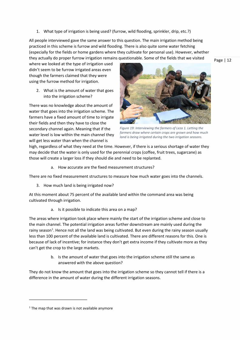
Figure 19: Interviewing the farmers of Leza 1. Letting the farmers draw where certain crops are grown and how much land is being irrigated during the two irrigation seasons.

Page | 13

4. What type of crops are grown and what is the approximate area of each crop in comparison with the area of land being irrigated? (%)

The data that we gathered from this was so unclear that it was a hard to know if it was really accurate. The way they knew how much they had was just through guessing what they harvested, or by looking what the amount was last year and then increasing it. Also no one really had the data we were looking for as the BoA of Finote Selam only had the sum of the whole area they are in charge of and didn’t have the data per irrigation area, (which was the data that was needed). Eventually the Kebele of Leza 1 gave us some data, but it was still unclear how this data was gathered. The main crops grown in this area however where: sugarcane, onions, potato, maize, and coffee. It seems like if you really need this information you have to calculate and collect the data yourself.

a. Is it possible to indicate the area for perennial and annual crops? (If they have both types.)

They couldn’t give us the exact location of the perennial and annual crops. This could be gathered by visiting all the sites but there was no time for it. It seemed that the perennial crops where mainly situated close to the main channel.

b. Do they use crop rotation?

They use crop rotation, but only for the annual crops. With crop rotation they also have a year when beans are planted which don’t give a large harvest, but this will improve the soil so the crops that are grown afterwards get an increase in yield. This is something that the DA of the area tries to teach the farmers.

c. How is the access for cash crops (perennial crops)?

The access to cash crops is quite okay. The only problem that the farmers face was that they first need to gather the money to be able to afford the seeds. When they have perennial crops they get priority with irrigation when the water level is too low to let all the farmers irrigate all their land. Only the fields where the perennial crops are grown are then irrigated. However the connection to the market is in some cases a bit hard which means that the farmers do not get as much profit as could be possible if this was improved.

5. How is the water being distributed between al the farms?

The water is being distributed between the farmers by every village individually. The amount of water that the village gets has to do with the number of residents inside the village. Each farmer gets half an hour of irrigation water, regardless of the size of his field or the type of crops being grown. The villages then decide the rotational scheme as to what time the fields are being irrigated. They irrigate 24 hours a day, meaning that some farmers have to irrigate during the night. In some villages female farmers have the privilege that they only get time slots to irrigate during the day, because of safety reasons, but this is not the case in all the villages.

a. Is this with time slots or by amount of cubic meters?

The amount of irrigated water is for every farmer only half an hour, regardless of his or her field size, crop or anything else.

6. How are these decisions being made about the irrigation scheme and the amount of water each farmer gets?

a. Who makes the decision how much water each person gets?

Page | 14

Figure 20: Some farmers of Leza 1 irrigation scheme who were interviewed

This has been decided by the water boards of the different villages a long time ago and hasn’t changed. This might change when the new irrigation scheme is established.

b. and what happens if someone takes more or less? Who checks?

They get a large fine. The villagers themselves check each other and would bring people to the water board if they take water when it is not their turn. However, we are told that apparently there are hardly ever people who steal water. It is not clear if this is truly the case or if they were referring to the situation now, when there is enough water.

c. What happens if the water availability is limited (e.g. If there is not enough water in the reservoir?)

When this happens they decide to give priority to the perennial crops.

7. What type of help do you give/get from the farmers/water board/BoA office (DA)? a. Do you feel like something is missing?

They give workshops on different topics, how to cultivate certain crops, how to protect plants against diseases etc. The only aspect which could be improved is the support for identifying the diseases and pesticides. Now there is only one expert for a whole region, which isn’t enough. He can never reach all the farmers and check their fields.

8. What are in your opinion the restrictions/problems that should be solved to increase the efficiency of the irrigation scheme?

According to the farmers, lining of the channels would ensure that there is less seepage. Also more access to pesticide/herbicides and fertilizers would help, and an increase in the education of all the farmers in the way of learning what is the most efficient way of irrigation. How for instance they can calculate the Crop Water Requirement. These are the possible solutions that the farmers gave.

Page | 15

Observation

When walking along the river and the main channel there were various activities that took place in or around the water. At several occasions we observed that livestock used the water of the river and channel to drink (figure 21-1). There did not really seem to be specific places which were allocated for the animals to use for watering. Washing clothes and themselves is also an activity which people do in the river upstream of the main channel. This could mean that the water used for irrigation has some chemicals which may damage the crops. Another reason why this may be dangerous is because the water is also being used as drinking water. Figure 21-4 shows how a boy was taking some water from the river, downstream of where they were cleaning clothes.

1 1 1 2

1 3 1 4

Figure 21: The different activities occurring in this irrigation scheme. 1- Livestock Watering. 2- Water Fetching for farming purposes. 3- Washing clothes and body. 4- Fetching water.

Page | 16

Throughout the irrigation scheme one could find areas where seepage was occurring. This could be a problem in periods when there is not enough water for all the irrigated land. The seepage is happening due to channels not being constructed properly and water leaking through the sides (figure 28 – 2) or due to the fact that there is hardly any current through the main channel (figure 22-1).

Another problem causing seepage is with the dams created before the main channel starts (figure 22-4). These two dams should direct the water towards the channel, but this is not the case. Also some of the distribution structures are broken and let through a lot of water (figure 22 – 3). Every time the farmers downstream have to irrigate they first need to close this with bags of sand. However, the farmer installed these structures themselves and it does show initiative to try and decrease seepage.

1 1

1 5 1 6

1 3 1 4

1 2

Figure 22: Water seepage problems and solutions. 1- Overflow, no clear bed of the main channel. 2- Seepage into secondary channel. 3- Broken intake causing a lot of water seepage. 4- Natural rivers. 5- Plastic to control the amount of seepage. 6- A properly maintained weir decreasing the amount of seepage.

Page | 17

There are already measures being taken by individual farmers to decrease the amount of seepage inside the main channel, such as using plastic sheets inside the channel through which the water can’t infiltrate (figure 22- 5). Or well-maintained weirs that are not broken and will only be opened when the farmer is irrigating his or her land.

When walking past the irrigation scheme there were also some other aspects which caught my attention, which could have an effect on the water flow of the channel. There was quite some floating material in the channel which could decrease the flow of the channel (figure 23 – 1). Also there were only a few places where you could pass the main channel, and the bridges that were constructed where mainly only for people. Animals have to go through the channel. This could cause damage to the side slopes of the channels (figure 23 – 2). Not only animals pass through the channel, but at some places you could see that vehicles had to pass through the channel causing damage

1 3

1 5 1 4

1 2 1 1

Figure 23: Extra observations. 1- Obstacles in the main channel. 2- Traditional bridges over the main channel. 3- The new irrigation channel used to expand the irrigated area. 4- How data is being archived in the Woeda Bureau of Agriculture connected to Leza 1 and 5- The main channel and the dam made to divert the water from the river to the main channel.

Page | 18

Figure 24: Adding fertilizer to the crops.

(figure 23 – 3). It was also said that the main channel started at the first dam, but when we walked a bit further you could find another place where another dam was created to ensure that the water didn’t go back into the natural river (figure 23 – 5).

When we went to the Woreda Bureau of Agriculture connected to Leza 1 it was shocking to see how the data was archived. Figure 23 – 4 shows how this was done. Hardly anything was saved digitally. The problem with this is that it becomes quite hard to know if the data that they have is actually accurate and quite often if you want to know something they could not find the information that you were asking for. It could also help to ensure that if something happens, such as a fire, they do not lose all their data. And at the same time it becomes easier to actually do something with the data afterwards, for instance identify trends. However, for this to actually have any great consequence the way that data gathering and validation, verification and management is being conducted should become more transparent and accurate.

Page | 19

Methodology 2 (Extra measurement work July 2016). When my first assignment (January-February 2016) at SMIS Bahir Dar was finished, I still really wanted to use the Dilution-Gauging method with an EC Meter to measure the river flow. The reason why this was still on my “to do list” was because during the field work it became evident that certain rivers/channels were really hard to use the Current Meter or the floating method. The reason for this was for instance because there were a lot of rocks constantly distributing the water, and low water discharge. Such a river could be seen in figure 25. It was not possible to calculate this discharge due to the fact that both the current meter and the floating method could not be applied. It would have been nice to be able to calculate this discharge measurement as the river flow measurements right before and after the diversion dam in front of this river were already conducted. However, there were no hand-held EC (Electric Current) meters which I could use to measure the discharge during my first stay in Bahir Dar. When I came back in July we brought an Electric Conductivity meter so I could do my experiment.

Figure 25: River after first dam at the Leza 1 Scheme.

Page | 20

Fieldwork When we went to collect the data we encountered several problems which resulted in the need to change our methodology. One of these was that the electric conductivity measuring stick that we used could not save the data automatically. This meant that the data was not as accurate as wished. Also this meant that the sampling location was not precisely the centre of the channel (in the middle and halfway down in the stream). But more of this will be discussed in the conclusion. Figure 26 shows the stream used for experiment 1.

The method we used in the field The method we used was different than intended due to the lack of certain materials. The method we used is:

1. Taking plastic cups and numbering them. 2. Measuring the salinity of the stream and writing this down. 3. Gathering 1.5 liter of stream water in a water bottle. 4. Adding 2 tea spoons of salt into the water bottle. 5. Mixing the salt and the water until it completely dissolved. 6. Measuring the salinity of the water bottle with salt. 7. Marking the start and the end of the trial river (at least 20 meters long). 8. At the same time of adding the salted water in the water bottle to the stream take the first

cup of water from the end position of the stream (cup number 1). 9. Every 5 seconds take a cup of water from the stream (going from cup number 1, 2, 3, etc.). 10. When all the water is taken measure the salinity in each cup and write down the results.

NOTE!: after each measurement properly clean the measuring tool with the stream water to neutralize it.

11. Measure the depth at different intervals of the stream length, plus the width of the channel at different places.

The methodology I used can be found in Annex 3. It is based on the Gooseff Hydroecology Science & Engineering Lab at Colorado State University.

Figure 26: The stream used for experiment 1

https://goosefflab.wordpress.com/


Page | 21

Outcome Data Experiment 1 In the graph below (graph 1), you can see that there is no clear line showing the change in the salinity which is found within the river flow (Annex 4). This is not how the graph should have looked. Graph 2 shows how the graph is supposed to look like to ensure that the data collected was correct. With this graph it becomes very hard, or not possible, to calculate a true discharge. This tells me that something went wrong with this experiment.

Possible Problems There are different aspects which could have caused the data to not be as expected. The first reason that I will mention is that we did not use enough salt for this particular stream. This seems to be the most logical answer to what went wrong. Looking back at the experiment one can calculate that we added 40 times less salt than the prescribed amount! This is definitely not enough and would account for the seeming lack of extra salinity in the stream. Therefore, because there was not a lot of salt added to the water it might be that the difference of salinity measured by the EC meter of the water of the stream did not change that much as it spreads throughout the whole stream. It needs extremes to be able to measure the peak flow of the salinized water and hence calculate the stream discharge.

The second reason could be that we didn’t measure long enough and that therefore our data didn’t go back to zero yet. This is clearly visible in graph 1, where you can see that the outcome does not go back to the base line. Also if you look at the results in the table shown in annex 3 you see that the last input of data was suddenly again relatively more saline than the rest. However, I do not believe that this was the case. As to ensure that this would not be a problem again it would be smart to first do a quick floating test to see how fast the leaf goes from the intake towards the measuring location

Graph 2: Data output of experiment 1. The amount of salt inside the river at a certain time.

Graph 1: How the graph is supposed to look like.

Page | 22

so that you have a rough estimation as to how long you at least have to conduct your measurements.

A third reason why the data wasn’t as accurate could have to do with communication. It seemed that the team didn’t understand me in the beginning when I tried to explain to them when and how they should take the cups of water from the river. This made the data in the first three cups a bit inaccurate. Another problem with the sampling of the water for the measurements was that we did not take the water exactly from the middle of the stream, and only from the top part of the stream. Even though the measurements should be made from the middle of the stream, halfway into the stream. This could have caused problems with the outcome of the data.

The final reason why the data may not be as accurate as hoped for is because the EC measurement tool was not accurate enough, and it could not log the results automatically at a given time interval. It might be that the conductivity measurement tool that we have used in this text experiment is actually not suitable for this type of measurements. In the experiment done in Iceland (Annex 3) an Onset HOBO U24-001 Conductivity Logger was used, this might be a better tool to use than the one that we have used (EC/TDS hydrotester model COM-80).

Page | 23

Outcome Data Experiment 2

Figure 27: The infiranz river.

To try to solve the problem with the data collected the first time using the EC meter as measuring device, the same experiment was repeated at the natural stream called Infiranz the way to Zege (figure 27). However, this time we used significantly more salt than the previous time. 1 kg of salt was mixed with 12 liter of stream water. Another aspect which was done differently was to first test how fast the river flow was. This was done using the floating method to see how fast it took to travel the distance of 10 meters which had been set out. This took about one minute. Therefore the measuring started after one minute. For the rest we kept the same procedure of first measuring the natural conductivity of the water, which was 94ppm. Then dissolving all the salt in the 12 liter of stream water, and adding the whole content and rinsing the material afterwards to ensure that all the salt went into the stream.

Graph 3: Data output of experiment 2. The amount of salt inside the river at a certain time.

As you can see from graph 3 there does now seem to be a very clear peak in the measured ppm of the river flow. This gives us the feeling that the data collected is more accurate. Also the discharge measured which is 705.362 L sec-1 seems to be more accurate than with experiment 1. This gives the impression that the reason why experiment 1 did not work was because of the little amount of salt added to the water.

monitor point: 10 minjection point: 0 m

ec probe: EC_04slug in: 13:55:00 HH:MM:SS

1st arrival: 13:55:00 HH:MM:SSbackground: 94.00 mS cm-1

peak time: 13:55:12 HH:MM:SSpeak cond: 149.00 mS cm-1

peak conc: 74.50 mg L-1

end monitoring: 14:07:58 HH:MM:SSmodal v: 0.833 m sec-1

slug mass: 992.1 g0th moment: 1406.497 mg L-1 sec

discharge: 705.362 L sec-1

t adv 00:00:12 HH:MM:SS

Page | 24

One aspect which makes the data gathered a bit strange are the two sudden peaks occurring when the ppm measurement was going down (see graph 3). I do not really know why this occurred and what the actual reason for this was, though a lack of full mixing could be responsible. This might be checked and confirmed if more of these experiments using this method are carried out. Repeating the measurement will help to give a clearer picture as to the end results. Especially if unexpected disturbances occur like the cows who came to drink from the stream (figure 27).

An aspect which might help to improve this data collection method even more would be if the time laps between the measurements taken of the ppm inside the river flow was done closer together to ensure that the outcome of especially the peak period would have been more precise. Also it would have helped if the measurements would have started a bit before the one minute after the salty water was added to the stream as the ppm measurement now taken started at 97 ppm (annex 3). The neutral measurement of the ppm was 94 ppm. This means that already some of the salted water might have passed through before the one minute laps times. Thirdly, repeating the experiment at least three times will ensure that the data collected is as accurate as possible and will decrease the chance of uncertainty. Finally, it might be useful to measure the ppm inside the cups during the sampling already, to ensure that the data seems to be accurate or not.

Figure 28: How the samples were collected. Figure 29: Measuring the ppm inside each sample.

Figure 30: Writing down the results

Page | 25

Conclusion Looking at the outcome of all the data it shows once again that the information gathered is not always what you expect. It is really hard to find a correlation as to which method is the most accurate as the difference between the methods is constantly changing. One aspect which seemed to be constant the whole time is that the Current Meter has usually the lowest m³/s. except at point 3. There are various possible reasons for this change, but one reason for this might be because the channel was not that deep at that point so when using the floating method it was a bit harder for the materials to float an not be disturbed by the vegetation in the channel.

In addition, if you look at the numbers it seems as if there is no seepage of water from point 3 until point 5. This is quite interesting as it would suggest that something has changed from these two measurement areas. However, you need to look at the numbers and the discharge difference is only 0.0002 increase of discharge from measuring point 3 to measuring point 5, so it might also just be a measurement error. To ensure that this is really not the case it is important to repeat the measurements and check whether there is a similar difference again.

Correspondingly the controlled method inside the university flume had some problems as explained in the chapter about results. This means that this method should ideally be repeated to ensure that the data collected is more accurate and that we can actually say something about the outcome of the measurement. This is something for future research.

From the interviews and the observations in the field it became clear that it is very important to work together with the farmers within the scheme, to check how they are using the irrigation channels now, and hence what functions the channel should need in the future. This is a strong aspect of the SMIS project. Also it showed that not only lining the channels and modernizing the irrigation scheme is needed. It also indicates that farmers within Leza 1 irrigation scheme need more education on how to irrigate their land properly (CWR), how to identify pests and diseases, what to do when they occur, how to prevent them, etc. With this knowledge the yield gap would decrease creating a larger and better quality harvest and an increase in income for the farmers.

As for the EC meter method for calculating the water discharge, there are still follow-up steps which need to be taken to ensure that the data collected using this method is more reliable and understandable. The use of this method of conducting this research would be very interesting and useful, especially for all the streams which are not suitable for the float or current meter method.

Discussion and Reflection There are certain limitations towards my research and eventually the results. One of these is that it would have been better if I could have visited the irrigation scheme beforehand to decide where I would do the discharge measurements. This would have ensured that I would have had more time to do the actual measurements in the field. This was also the case when conducting the EC meter method as finding the right channel/river/stream close to Bahir Dar for this type of experiment was harder than was expected beforehand.

This brings me to the second aspect. Due to the lack of time in the field the total amount of field research was limited; it would have been better if there was more time for the measurements. For future research on this topic I would really recommend to increase the amount of time available for field work.

Thirdly, the results from the measurements done in the flume at the university do not seem to be correct. It is still unclear what went wrong, but I would like to have repeated the research as this

Page | 26

dataset is quite important to identify the accuracy of the different measurement methods we used. When I returned on my second visit I was told that the flume was not accurate and that using the floating method would be more accurate than the flume. This directly gives a idea as to the assumptions of university staff on how accurate the flume is.

Finally, using the EC meter to calculate the discharge was something new for me and something that I had not tried before or had seen done. This ensured that I virtually needed to start from scratch. As this was the case, the first time doing the experiment was very clumsy and not as accurate as I had hoped for. In addition the measurements were done during the rainy season. Which meant that getting to the rivers/streams was quite hard and also finding the right type of river/stream seemed to be a challenge.

Recommendations There are a lot of aspects which I would recommend for additional research. As I hardly had enough time to do my research properly I would recommend that there is further and more thorough research being done on discharge measurement tools in order to get an idea which one is the most accurate an precise to use for the irrigation schemes in Ethiopia.

Furthermore it would be really interesting to measure the discharge of the Leza River throughout the entire dry season. For instance to do measurements each month at the same locations. This would give a better idea of the possibilities of the irrigation scheme, the water availability. The farmers now said in the beginning that the river nearly always has the same amount of discharge. Yet, at the same time they do tell that when the water from the river is low they only irrigate the perennial crops. This then seems to indicate that there is a difference in the amount of water available from the river.

The above could be facilitated by installing a simple V-notch weir in the main channel, at which it would be comparatively simple to measure the discharge. This would also allow comparison with the various other methods in a more straightforward manner.

It would have also been really interesting to create a map of how the traditional irrigation scheme is now. Especially because the farmers say that there are different places where spring water comes in and joins the main channel ensuring that the water discharge increases again. Now it is unknown where these springs exactly are and if they are actually within the Leza 1 irrigation scheme or only at the end of the irrigation scheme. This would be interesting especially as it seemed as if there was an increase in water towards the end of the main channel. This could be because of inaccuracy of the measurements. But it is also possible that there is inflow of groundwater. If this is the case then the irrigation channel should not be lined at those areas.

Fourthly I would recommend to study how and even if knowledge, of which there is a lot of in Ethiopia, reaches the famers. Not only in the context as to how the governmental institutes are operating, but also how they choose to give which trainings. There is already a quite vast explanation as to the dissemination of information within Ethiopia. However, it is not clear in what cases this process is going well and where there may be room for improvements. It would also be interesting to find out the attitude of the farmers towards those DA’s working for the Bureau of Agriculture.

As for the Dilution-Gauging method with an EC Meter there are also various studies which should be done to get a better understanding of this relatively new and rather unknown way of calculating discharge. These possible research topics are:

Page | 27

• Try the same experiment with even more salt. • Increase the frequency of sampling, especially around the peak of the salinity, to capture

this peak more accurately • Measure the water salinity for a longer period of time. • Take the measurements of the salinity in the centre of the channel. • If possible try to get an EC meter which saves the data automatically at given time intervals. • Try the same experiment with two EC meters and keeping them inside the water and every

time the seconds have passed click on hold take that EC meter out of the water and write down the salinity of the water. At the same time put the other EC meter into the water so that when the next measurement needs to be done the measurement is stable.

• Try the methodology on different irrigation channels, streams, etc.

These are the different studies which I believe should really be done to ensure that there is a more thorough understanding of this method and to see whether this method is applicable in Ethiopia, and if yes, under which circumstances.

Figure 31: The main channel of Leza 1

Page | 28

References Environmental field techniques: Stream Discharge measurement I: Float and Velocity-Area Methods <http://www.colorado.edu/geography/courses/geog_2043_f01/lab 01_2.html> date of : 11/07/2016

New, D., (2005) Measuring Head and Flow. <http://www.homepower.com/articles/microhydro-power/design-installation/intro-hydropower-part-2> 01/02/2016

Michaud, J. P. & Wierenga. M., (2005) ESTIMATING DISCHARGE AND STREAM FLOWS: A Guide for Sand and Gravel Operators. Washington State Development of Ecology.

Wlostowski, A. N., Smull, E. M., Gooseff, M.N., (2012). Measuring Discharge With Conservative Trachers.<https://goosefflab.wordpress.com/2012/07/26/measuring-discharge-with-conservative-tracers/> the Gooseff Hydroecology Science & Engineering Lab at Colorado State University

http://www.homepower.com/articles/microhydro-power/design-installation/intro-hydropower-part-2

http://www.homepower.com/articles/microhydro-power/design-installation/intro-hydropower-part-2


Page | i

Annex 1 1.1 Methodology 1.1.1 Methods used to calculate the water flow in the irrigation scheme Where to conduct the measurements in an irrigation scheme When conducting the measurements it is important to choose the right spot. There are different guidelines for choosing the right spot, but for this research measurements will be taken, if possible, at each change of flow within the irrigation scheme. Thus, where the irrigation scheme starts, the main channel, the secondary channel, etc.

To get the best results it would be recommended to do the measurements at three points at each of these changes (see the sketch in figure 32). That way you can find out how accurate your measurements are. For instance, the sum of the water discharge at point 2 and 3 should equal the water discharge at point 1.

Floating method: To use the floating method it is very important that you choose a good and representative part of the irrigation scheme to do the measurements. Conditions that you should keep in mind when selecting the gauging site are:

o The reach should be straight. o Channel width should be relatively uniform along the reach. o Channel cross section shape should be relatively uniform along the reach. o Flow direction should be parallel with the channel sides along the reach, with no eddies or

stones or stagnant (‘dead’) water. o The channel should be clear and unobstructed by trees, aquatic growth or other obstacles. o Sites subject to backwater effects by downstream obstacles should be avoided. o All of these conditions mentioned should be valid for at least a length of 5 meters from the

different locations of the irrigation channel that you want to measure. After this has been done you first start with measuring the geometry of the reach (see figure 33):

1. Measure the length of the reach in meters between the upstream and the downstream cross sections using a surveyors measuring tape. The length of the reach should be a minimum of 3 meters and may be up to 10-15 meters longer if the channel conditions are constantly the same.

2. Measure the width of the irrigation channel by recording the width of the water surface with a measuring tape at different verticals alongside the reach of your experimental area.

3. At each of those points, measure the depth at regular verticals across the channel using a steel tape and calculating an average depth. Use a board that can span across the whole channel and mark it at 0.2 m verticals. Lay the board across the stream, and measure the stream depth at each 0.2 m interval. To compute the average depth, add all of your measurements together and divide by the number of measurements you made.

4. The cross section area is measured multiplying the width by the mean depth. 5. Enter the geometry data into the excel file.

Figure 32: Where to do the measurements

Page | ii

Figure 33: Floating method

When all the geometry measurements have been completed the calculations for the velocity of the water will be executed. This will be done through the following steps:

1. Use a weighted float that can be clearly seen—an orange or grapefruit works well. 2. Place it well upstream of your measurement area, and use a stopwatch to time how long it

takes to travel the length of your measurement section. Start the stopwatch when the float crosses the upstream cross section. This can be signalled by spanning a string across the water at the upstream cross section to ensure that the data will become more accurate (see figure 33). Do the same for the downstream cross section.

3. Repeat this several times. Minimum of 3, but if the data collected varies a lot keep on repeating the measurement until there is not too much variation between the different values. The stream speed probably varies across its width, so measure the time for different locations spaced at regular verticals across the channel

4. Calculate the average water velocity by dividing the length of the reach by the average travel time. Note that this figure is an average velocity for the water at the surface at the stream. Velocity decreases with depth to the stream bed. Therefore an average stream velocity should be computed by multiplying the average surface velocity by a velocity coefficient. The velocity coefficient may be assumed to take the value 0.65. Note that the velocity coefficient may be computed by measuring actual average stream velocity with a current meter and dividing this by the surface velocity measured with the float.

5. Enter the velocity data into the field form in the excel file.

http://www.homepower.com/sites/default/files/articles/ajax/docs/08_HP104_pg42_New-4.jpg Extracted on: 01/02/2016

Page | iii

The traditional method that is mainly being used in the field in Ethiopia is the floating method. For this method one usually finds something that can float, for instance a piece of bamboo or a leaf (these are most commonly used). However, these methods are not the most accurate as it will ensure that you only measure the top part of the whole channel. And because these objects float directly on the surface they will be influenced more by other elements such as the wind (figure 34). To identify if there really is a difference in calculating the water discharge into the channel using other materials than the traditionally used ones, the floating method will be conducted and different floating materials will be used to find out if the outcome varies between the different floating materials. The materials that will be used are:

o An orange o A plastic water bottle o A wine bottle o A leaf

Not all of these methods will be tested at each place as not all the methods may be possible to do due to the conditions of the channels.

Current meter: Wading method:

The wading method involves having the hydrographer stand in the water holding a wading rod with the current meter attached to the rod. The wading rod is graduated so that the water depth can be measured. The rod has a metal foot pad which sits on the channel bed. The current meter can be placed at any height on the wading rod and is readily adjusted to another height by the hydrographer while standing in the water (see figure 35).

1. First the width of the channel is being calculated perpendicular to the flow direction from one edge of the water to the other one.

2. Depending on the width, different numbers of verticals will be measured. Table 12 shows the different number of verticals in correspondence with the width of the channel.

Table 12: How to decide the number of verticals

Channel width (meters) 0-0.5 0.5-1 1-3 3-5 5-10 >10

Number of verticals 3-4 4-5 5-8 8-10 10-20 >20

3. At each interval point the depth is being measured and written down (see annex 1a). 4. Depending on the depth of the channel the calculations for how high the propeller needs to

be situated will need to be calculated. If the depth is lower than 0.5 meter then you simply

http://www.colorado.edu/geography/courses/geog_2043_f01/lab01_2.html

Figure 34: Different velocity in a channel

Figure 35: How to put the current meter inside the water

Page | iv

multiply the measured depth with 0.4. If it is deeper than 0.5 meter then you should multiply the measured depth with 0.2 and 0.8. The velocity of the water then needs to be calculated at two different heights at the same interval.

5. When these calculation are done and written down, the hydrographer standing in the water will use measuring tape strapped from one side of the channel to the other side of the channel as reference point as to where he needs to place the rod with the current meter attached to it.

6. BEFORE placing the wading rod in the water, adjust the height of the propeller so that it is the exact height as calculated.

7. The hydrographer stands 5-10 cm downstream from the measuring tape that is strapped across the channel and approximately 50 cm to one side of the wading rod.

8. During the measurement, the rod needs to be held in a vertical position and the current meter must be parallel with the flow direction.

9. When everything is in proper position the hydrographer can star the measuring and the results will be written down on the sheet.

10. Step 5 up to 9 will be repeated for each vertical measurement in the channel. 11. All data will be inserted in the excel sheet to calculate the exact discharge.

Controlled research of the different methods. When the measurements have been done in the field the exact measurement methods will be done again in a controlled environment. This will be at the University of Bahir Dar, in the hydraulics laboratory. As there will hardly be any other forces which may influence the outcome this test will give us a clearer understanding about the accuracy of each measuring method. Hence, helping us answer the research question which method is the most accurate.

1.1.2 Interviews The interviews will be semi structured interviews. The questions that I would like to raise are:

1. What type of irrigation is being used? (Furrow, wild flooding, sprinkler, drip, etc?) 2. What is the amount of water that goes into the irrigation scheme?

a. How accurate are the fixed measurement structures, if any? 3. How much land is being irrigated now?

a. Is it possible to indicate this area on a map? b. Is the amount of water that goes into the irrigation scheme still the same as

answered with the above question? 4. What type of crops are being grown and what is the approximate area of each crop in

comparison with the area of land being irrigated? (in %, rough estimate) a. Is it possible to indicate the area for perennial and annual crops? (If they have both

types.) b. Do the farmers use crop rotation? c. How is the market access for cash crops?

5. How is the water being distributed between al the farms? a. Is this with time slots or by volume (cubic meters)?

http://geographyfieldwork.com/Qmes.sch2.gif

Figure 36: Sketch of midsection: how to collect the data for the current meter

Page | v

6. How are decisions being made about the irrigation scheme and the amount of water each farmer gets?

a. Who makes the decision how much water each person gets b. and what happens if someone takes more or less? Who checks? c. What happens if the water availability is limited (e.g. If there is not enough water in

the reservoir?) 7. What type of help do you give/get from the farmers/water board/BoA office (DA)?

a. Do you feel like something is missing? 8. What are in your opinion the restrictions/problems that should be solved to increase the

efficiency of the irrigation scheme? 9. Is there anything else that you feel that I have left out and that you would like to tell me?

This is already quite elaborate. However, I do not need precise answers for each of these questions. During the interview I will start by asking them to explain how the irrigation scheme works and from what they then explain to me I decide which follow up questions to ask. This way the interview will gather the most interesting information as it will ensure that you get a clear understanding what the person you are interviewing really thinks and knows about certain topics. From that topic you then go to the next topic. Through this method you eventually go through all the different questions as stated in the above, and maybe some more questions will be answered.

1.1.3 Observations Observations will be done throughout the whole process. As I do not know a lot about Ethiopia and how things are done here, it is important to stay alert and constantly look around and make notes and photos of aspects that catch my interest.

This observation study will also be done when doing the floating and current meter method for finding the amount of water passing through the channel. I will try to gain an understanding what the normal procedure is for gathering this data and ask why the measurements are done in a certain way. Through this I hope to be able to trigger the experts to become more critical in their own research.

Also just walking through the irrigation scheme will be very useful to gather information as to the state of the scheme and what kind of problems it might face. Seeing how a farmer irrigates its land will also be very useful as it will directly give a first-hand experience to see how well they know how to irrigate their land. For example: if a farmer says he uses furrow irrigation, to check if it is really furrow irrigation or if it is more like wild flooding.

Page | vi

1.2 Data Sheet Current Meter Monitoring Location: Measuring time: 60 sec

Date/time: GPS data: N. S. El.

Staff gauge (m)

Vertical/ sub section

Distance on tape (vertical) (m)

Depth at vertical (m)

Observational depth (0.4D) (m)

No. of rev’s in measured period.

1 2 3 4 5 6 7 8 9 10 11 12 13 14 15 16 17 18 19 20 21 22 23 24

Notes:

Page | vii

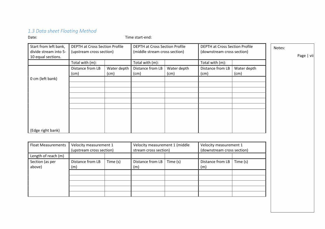
1.3 Data sheet Floating Method Date: Time start-end:

Start from left bank, divide stream into 5-10 equal sections.

DEPTH at Cross Section Profile (upstream cross section)

DEPTH at Cross Section Profile (middle stream cross section)

DEPTH at Cross Section Profile (downstream cross section)

Total with (m): Total with (m): Total with (m): 0 cm (left bank) (Edge right bank)

Distance from LB (cm)

Water depth (cm)


Water depth (cm)


Water depth (cm)

Float Measurements Velocity measurement 1 (upstream cross section)

Velocity measurement 1 (middle stream cross section)

Velocity measurement 1 (downstream cross section)

Length of reach (m) Section (as per above)

Distance from LB (m)

Time (s) Distance from LB (m)

Time (s) Distance from LB (m)

Time (s)

Notes:

Page | viii

Annex 2 Measurements taken on point 1: Main River

Date Amharic: 24/5/2008 Time at start: 10:48 Staff Gauge at start: noneDate Gregorian: 01/02/2016 Time at end: 03:36 Staff Gauge at end: none

Station: Leza ant (+/- 150 meters Upstream of the tradtional intace (orange)) Name of site manager: kabele DA (name?)

Start from left bank, divide stream into 5-10 equal sections

Total Width (metres): 3.4 Total Width (metres): 4 Total Width (metres): 3.6Distance from LB (cm) Water Depth (cm) Distance from LB (cm) Water Depth (cm) Distance from LB (cm) Water Depth (cm)

0 cm (Left bank) 0 0 0 0 0 050 25 50 10 50 4

100 26.5 100 14.5 100 7150 30 150 14.5 150 9200 27 200 13 200 9250 18 250 12 250 9300 8.5 300 9 300 6350 0 350 5 350 3

(Edge right bank)Mean depth (m): 0.169 0.10 0.06

Area of Cross section profile (m2): 0.57 0.39 0.21

FLOAT MEASUREMENTSLength of reach (metres): 8.2 8.2 8.2

Section (as per above) Distance from LB (m) Time (seconds) Distance from LB (m) Time (seconds) Distance from LB (m) Time (seconds)0 cm (Left bank) 0 0 0 0

50 50 50100 100 100150 22.59 150 22.59 150 22.59200 20.52 200 20.52 200 20.52250 20.6 250 20.6 250 20.6300 300 300350 350 350

(Edge right bank)Average no of seconds over the reach: 16 21 21

Average velocity for measurement 1 (m/s): 0.51 0.39 0.39

CALCULATION OF DISCHARGE (m3/s) OBSERVATIONS (weather, flow conditions, difficulties experienced during measurement)

Average cross section area: 0.392Average measured velocity (m/s): 0.43

Velocity coefficient: 0.65Average channel velocity (m/s): 0.28

Discharge (Flow) (m3/s): 0.109

DEPTH at Cross Section Profile 1 (upstream cross section)

DEPTH at Cross Section Profile 2 (middle cross section)

DEPTH at Cross Section Profile 3 (downstream cross section)

VELOCITY MEASUREMENT 1 VELOCITY MEASUREMENT 2 VELOCITY MEASUREMENT 3

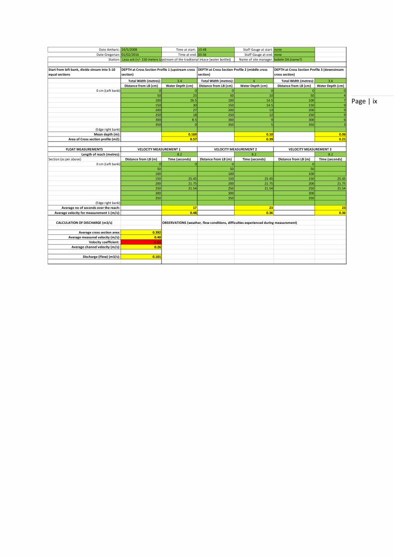
Page | ix

Date Amharic: 24/5/2008 Time at start: 10:48 Staff Gauge at start: noneDate Gregorian: 01/02/2016 Time at end: 03:36 Staff Gauge at end: none

Station: Leza ant (+/- 150 meters Upstream of the tradtional intace (water bottle)) Name of site manager: kabele DA (name?)


Total Width (metres): 3.4 Total Width (metres): 4 Total Width (metres): 3.6Distance from LB (cm) Water Depth (cm) Distance from LB (cm) Water Depth (cm) Distance from LB (cm) Water Depth (cm)

0 cm (Left bank) 0 0 0 0 0 050 25 50 10 50 4

100 26.5 100 14.5 100 7150 30 150 14.5 150 9200 27 200 13 200 9250 18 250 12 250 9300 8.5 300 9 300 6350 0 350 5 350 3



FLOAT MEASUREMENTSLength of reach (metres): 8.2 8.2 8.2

Section (as per above) Distance from LB (m) Time (seconds) Distance from LB (m) Time (seconds) Distance from LB (m) Time (seconds)0 cm (Left bank) 0 0 0 0

50 50 50100 100 100150 25.45 150 25.45 150 25.45200 21.75 200 21.75 200 21.75250 21.54 250 21.54 250 21.54300 300 300350 350 350











Page | x

Monitoring location: Leza ant 1.1 (+/- 150 meters Upstream of GPS dataDate: 2/01/2016 Northing:10.424793Time: 11 am (5 ethiopian time) Easting:37.372881Staff gauge (m): None Elevation: 1882 m above sea levelMeasuring Period (seconds): 60Vertical Dist on Width of Depth Area Observational No. of No. of Velocity Mean Vert. Mean Sub. Discharge Observations, including/ Sub- Tape Sub-section at Vertical Subsection Depth (0.4D etc) Revs in Revs / sec at point Velocity Sect. Velocity sediment samples

Section m m m m2 m Meas. Period n m/s m/s m/s m3/s

1 0 0.50 0.00 0.01 0 0 0.00 0.00 0.00 propellor partially above the water

0.00 0.00

2 0.5 0.50 0.04 0.03 0.025 50 0.83 0.43 0.22

0.00 0.00

3 1 0.50 0.07 0.04 0.028 52 0.87 0.45 0.22

0 0.00 0.00

4 1.5 0.50 0.09 0.05 0.036 62 1.03 0.53 0.27

0 0.00 0.00

5 2 0.50 0.09 0.05 0.036 72 1.20 0.62 0.31 the depth measured changed

0 0.00 0.00 because of the waves in the water.

6 2.5 0.50 0.09 0.04 0.036 86 1.43 0.74 0.37 propellor partially above the water

0 0.00 0.00

7 3 0.50 0.06 0.02 0.024 62 1.03 0.53 0.27 propellor partially above the water

0 0.00 0.00

8 3.5 -3.50 0.03 -0.05 0.025 0 0.00 0.00 0.00

0 0.00 0.00

9 0.00 0.00 0 0.00 0.00 0.00

0 0.00 0.00

10 0.00 0.00 0 0.00 0.00 0.00

0 0.00 0.00

11 0.00 0.00 0 0.00 0.00 0.00

0 0.00 0.00

12 0.00 0.00 0 0.00 0.00 0.00

0 0.00 0.00

13 0.00 0.00 0 0.00 0.00 0.00

0 0.00 0.00

14 0.00 0.00 0 0.00 0.00 0.00

0 0.00 0.00

15 0.00 0.00 0 0.00 0.00 0.00

0.00 0.00

16 0.00 0.00 0.00

0.00 0.00

TOTAL MEAN TOTAL MEAN TOTAL Carry over to another sheet ifWIDTH DEPTH AREA VELOCITYDISCHARGEnecessary. Repeat Vertical No. 16

m m m2 m/s m3/s at top of next sheet.TOTAL 0.00 0.06 0.18 0.11 0.060

0.00 0.000

0.00 0.000

0.00 0.000

0.00 0.000

0.00 0.000

0.00 0.000

0.00 0.000

0.32 0.012

0.13 0.003

0.00 0.000

0.25 0.010

0.29 0.013

0.34 0.015

0.11 0.001

0.22 0.006

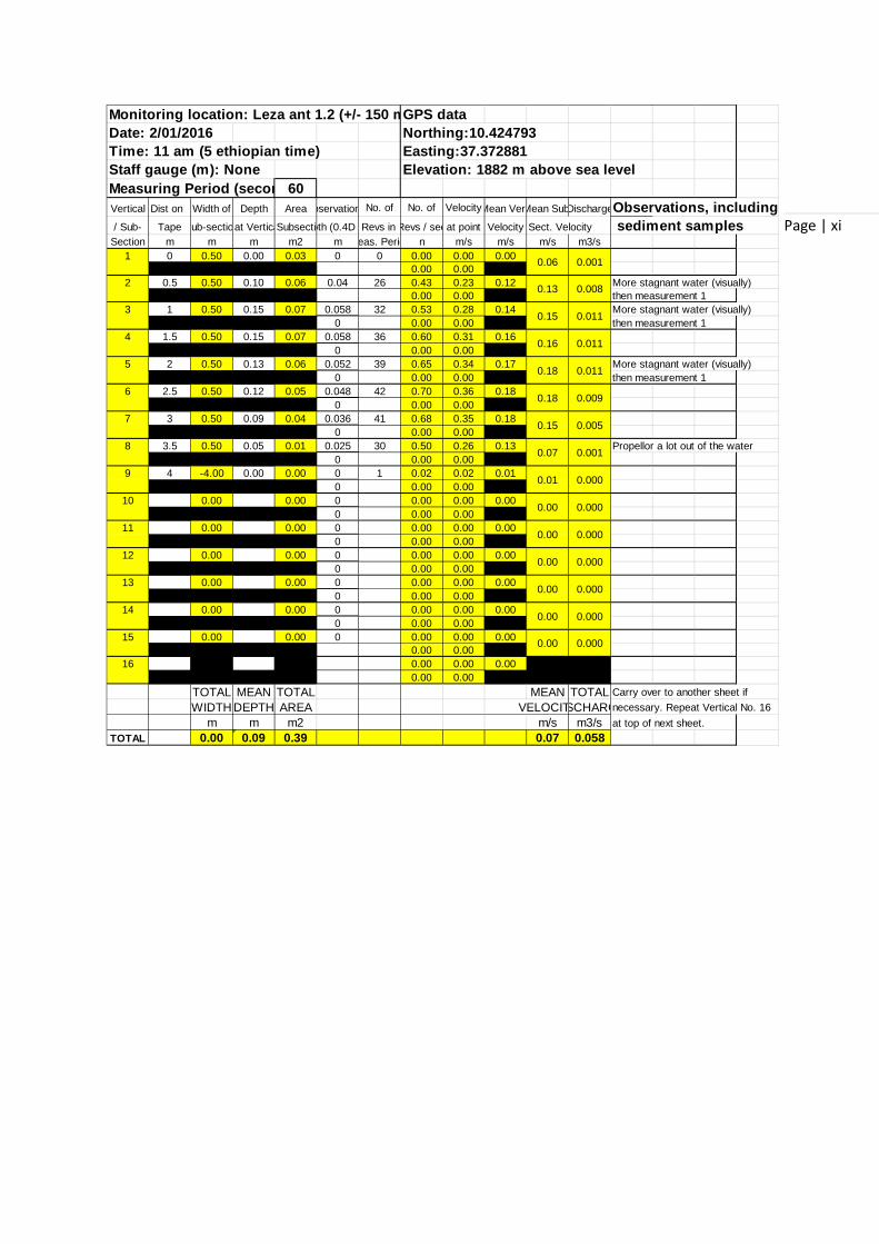
Page | xi

Monitoring location: Leza ant 1.2 (+/- 150 m GPS dataDate: 2/01/2016 Northing:10.424793Time: 11 am (5 ethiopian time) Easting:37.372881Staff gauge (m): None Elevation: 1882 m above sea levelMeasuring Period (secon 60Vertical Dist on Width of Depth Area bservation No. of No. of VelocityMean VertMean SubDischargeObservations, including/ Sub- Tape Sub-sectioat VerticaSubsectiopth (0.4D eRevs in Revs / secat point Velocity Sect. Velocity sediment samples

Section m m m m2 m eas. Perio n m/s m/s m/s m3/s1 0 0.50 0.00 0.03 0 0 0.00 0.00 0.00

0.00 0.002 0.5 0.50 0.10 0.06 0.04 26 0.43 0.23 0.12 More stagnant water (visually)

0.00 0.00 then measurement 13 1 0.50 0.15 0.07 0.058 32 0.53 0.28 0.14 More stagnant water (visually)

0 0.00 0.00 then measurement 14 1.5 0.50 0.15 0.07 0.058 36 0.60 0.31 0.16

0 0.00 0.005 2 0.50 0.13 0.06 0.052 39 0.65 0.34 0.17 More stagnant water (visually)

0 0.00 0.00 then measurement 16 2.5 0.50 0.12 0.05 0.048 42 0.70 0.36 0.18

0 0.00 0.007 3 0.50 0.09 0.04 0.036 41 0.68 0.35 0.18

0 0.00 0.008 3.5 0.50 0.05 0.01 0.025 30 0.50 0.26 0.13 Propellor a lot out of the water

0 0.00 0.009 4 -4.00 0.00 0.00 0 1 0.02 0.02 0.01

0 0.00 0.0010 0.00 0.00 0 0.00 0.00 0.00

0 0.00 0.0011 0.00 0.00 0 0.00 0.00 0.00

0 0.00 0.0012 0.00 0.00 0 0.00 0.00 0.00

0 0.00 0.0013 0.00 0.00 0 0.00 0.00 0.00

0 0.00 0.0014 0.00 0.00 0 0.00 0.00 0.00

0 0.00 0.0015 0.00 0.00 0 0.00 0.00 0.00

0.00 0.0016 0.00 0.00 0.00

0.00 0.00TOTAL MEAN TOTAL MEAN TOTAL Carry over to another sheet ifWIDTH DEPTH AREA VELOCITSCHARGnecessary. Repeat Vertical No. 16


0.06 0.001

0.13 0.008

0.15 0.011

0.16 0.011

0.18 0.011

0.18 0.009

0.15 0.005

0.07 0.001

0.01 0.000

0.00 0.000

0.00 0.000

0.00 0.000

0.00 0.000

0.00 0.000

0.00 0.000

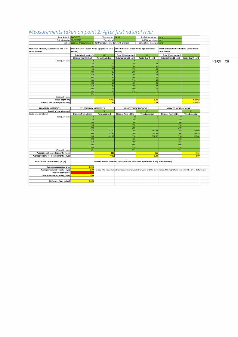
Page | xii

Measurements taken on point 2: After first natural river

Date Amharic: 24/5/2008 Time at start: 14:00 Staff Gauge at start: noneDate Gregorian: 02/01/2016 Time at end: Staff Gauge at end: none

Station: Leza Ant (Measurement 2, after frist natural river dam (with Orange)) Name of site manager: none


Total Width (metres): 5.71 Total Width (metres): 5.2 Total Width (metres):Distance from LB (cm) Water Depth (cm) Distance from LB (cm) Water Depth (cm) Distance from LB (cm) Water Depth (cm)

0 cm (Left bank) 0 0 050 19 50 34

100 27 100 50150 58 150 51200 63 200 52250 67 250 54300 65 300 52350 67 350 49400 61 400 46450 52 450 37500 36 500 16550 21 520 0571 0

(Edge right bank)Mean depth (m): 0.412 0.40 #DIV/0!

Area of Cross section profile (m2): 2.35 2.08 #DIV/0!

FLOAT MEASUREMENTSLength of reach (metres): 10 10 10

Section (as per above) Distance from LB (m) Time (seconds) Distance from LB (m) Time (seconds) Distance from LB (m) Time (seconds)0 cm (Left bank) 0 0 0 0 0 0

50 50 50100 100 100150 150 150200 200 200250 152.02 250 152.02 250 152.02300 143.85 300 143.85 300 143.85350 162.62 350 162.62 350 162.62400 400 400450 450 450500 500 500550 550 550

(Edge right bank) 571 571 571Average no of seconds over the reach: 115 115 115



Average cross section area: 2.220Average measured velocity (m/s): 0.09 The boy who helped with the measurements was in the water and the moved once. This might have caused a little bit of disturbance.







Page | xiii



0 cm (Left bank) 0 0 050 19 50 34

100 27 100 50150 58 150 51200 63 200 52250 67 250 54300 65 300 52350 67 350 49400 61 400 46450 52 450 37500 36 500 16550 21 520 0571 0





50 50 50100 100 100150 150 150200 200 200250 166.03 250 166.03 250 166.03300 178.75 300 178.75 300 178.75350 158.32 350 158.32 350 158.32400 400 400450 450 450500 500 500550 550 550




Average cross section area: 2.220Average measured velocity (m/s): 0.08 The boy who helped with the measurements was in the water and the moved once. This might have caused a little bit of disturbance.







Page | xiv


Station: Leza Ant (Measurement 2, after frist natural river dam (with Water Bottle) Name of site manager: none



0 cm (Left bank) 0 0 050 19 50 34

100 27 100 50150 58 150 51200 63 200 52250 67 250 54300 65 300 52350 67 350 49400 61 400 46450 52 450 37500 36 500 16550 21 520 0571 0





50 50 50100 100 100150 150 150200 200 200250 145.98 250 145.98 250 145.98300 181.16 300 181.16 300 181.16350 147.07 350 147.07 350 147.07400 400 400450 450 450500 500 500550 550 550




Average cross section area: 2.220 The boy who helped with the measurements was in the water and the moved once. This might have caused a little bit of disturbance.Average measured velocity (m/s): 0.08







Page | xv

Measurements taken on point 3: After both natural rivers in the main channel


Station: Leza Ant (Measurement 3 near the second natural river dam (with Orange)) Name of site manager: none



0 cm (Left bank) 0 0 0 0 0 020 19 20 1840 29 40 2460 30 60 2680 28 80 27

100 24 100 20120 17 120 0140 0




Section (as per above) Distance from LB (m) Time (seconds) Distance from LB (m) Time (seconds) Distance from LB (m) Time (seconds)0 cm (Left bank) 0 0 0

20 21 20 21 20 2140 21.81 40 21.81 40 21.8160 20.5 60 20.5 60 20.580 20.01 80 20.01 80 20.01

100 21.29 100 21.29 100 21.29120 22.02 120 22.02 120 22.02140




Average cross section area: 0.151Average measured velocity (m/s): 0.24 Some grass

Velocity coefficient: 0.65 a lot of other leafs and other materials floating in the water.Average channel velocity (m/s): 0.15







Station: Leza Ant (Measurement 3 near the second natural river dam(With Wine Bottle Name of site manager: none



0 cm (Left bank) 0 0 0 0 0 020 19 20 1840 29 40 2460 30 60 2680 28 80 27

100 24 100 20120 17 120 0140 0





20 26.4 20 28.4 20 28.440 25.86 40 25.86 40 25.8660 24.25 60 24.25 60 24.2580 24.45 80 24.45 80 24.45

100 25.56 100 25.56 100 25.56120 27.96 120 27.96 120 27.96140




Average cross section area: 0.151 Some grassAverage measured velocity (m/s): 0.19 a lot of other leafs and other materials floating in the water.







Page | xvi


Station: Leza Ant (measurment 3, near the second natural river dam (with Water Bottl Name of site manager: none



0 cm (Left bank) 0 0 0 0 0 020 19 20 1840 29 40 2460 30 60 2680 28 80 27

100 24 100 20120 17 120 0140 0





20 25.32 20 25.32 20 25.3240 19.63 40 19.63 40 19.6360 18.35 60 18.35 60 18.3580 18.16 80 18.16 80 18.16

100 19.68 100 19.68 100 19.68120 24.8 120 24.8 120 24.8140




Average cross section area: 0.151Average measured velocity (m/s): 0.24 Some grass

Velocity coefficient: 0.65 a lot of other leafs and other materials floating in the water.Average channel velocity (m/s): 0.15







Station: Leza Ant (Measurment 3, near the second natural river dam (with Leaf)) Name of site manager: none



0 cm (Left bank) 0 0 0 0 0 020 19 20 1840 29 40 2460 30 60 2680 28 80 27

100 24 100 20120 17 120 0140 0

(Edge right bank)Mean depth (m): a 0.184 0.16 0.00




20 20 2040 19.01 40 19.01 40 19.0160 18.9 60 18.9 60 18.980 17.76 80 17.76 80 17.76

100 18.84 100 18.84 100 18.84120 18.85 120 18.85 120 18.85140




Average cross section area: 0.151 Some grassAverage measured velocity (m/s): 0.27 a lot of other leafs and other materials floating in the water.







Page | xvii

Measurements taken on point 4: Secondary channel

Monitoring location: Leza ant 3. (point 3 main channel after s GPS dataDate: 3/01/2016 Northing:10.720966Time: 10 am Easting:37.362718Staff gauge (m): None Elevation: 1827 m above sea levelMeasuring Period (seconds): 60Vertical Dist on Width of Depth Area Observational No. of No. of Velocity Mean Vert. Mean Sub. Discharge Observations, including/ Sub- Tape Sub-section at Vertical Subsection Depth (0.4D etc) Revs in Revs / sec at point Velocity Sect. Velocity sediment samples


1 0 0.20 0.00 0.02 0 0 0.00 0.00 0.00

0.00 0.00

2 0.2 0.20 0.18 0.04 0.072 21 0.35 0.19 0.09 Grass on the side effected the

0 0.00 0.00 outcome

3 0.4 0.20 0.24 0.05 0.096 33 0.55 0.29 0.14

0 0.00 0.00

4 0.6 0.20 0.26 0.05 0.104 33 0.55 0.29 0.14

0 0.00 0.00

5 0.8 0.20 0.27 0.05 0.108 33 0.55 0.29 0.14

0 0.00 0.00

6 1 0.20 0.20 0.02 0.08 28 0.47 0.25 0.12

0 0.00 0.00

7 1.2 -1.20 0.00 0.00 0 1 0.02 0.02 0.01

0 0.00 0.00

8 0.00 0.00 0 0.00 0.00 0.00

0 0.00 0.00

9 0.00 0.00 0 0.00 0.00 0.00

0 0.00 0.00

10 0.00 0.00 0 0.00 0.00 0.00

0 0.00 0.00

11 0.00 0.00 0 0.00 0.00 0.00

0 0.00 0.00

12 0.00 0.00 0 0.00 0.00 0.00

0 0.00 0.00

13 0.00 0.00 0 0.00 0.00 0.00

0 0.00 0.00

14 0.00 0.00 0 0.00 0.00 0.00

0 0.00 0.00

15 0.00 0.00 0 0.00 0.00 0.00

0.00 0.00

16 0.00 0.00 0.00

0.00 0.00



NOTES: There where quite some leaves and other floating materials in the water Observer Date

0.05 0.001

0.12 0.005

0.14 0.007

0.14 0.008

0.13 0.006

0.07 0.001

0.01 0.000

0.00 0.000

0.00 0.000

0.00 0.000

0.00 0.000

0.00 0.000

0.00 0.000

0.00 0.000

0.00 0.000

Page | xviii

Measurements taken on point 5: More downstream of the main channel


Station: Leza Ant (Measurment 5, down the main channel 1 km from point4 (Orange)) Name of site manager: none


Total Width (metres): 1.3 Total Width (metres): 1.6 Total Width (metres): 1.5Distance from LB (cm) Water Depth (cm) Distance from LB (cm) Water Depth (cm) Distance from LB (cm) Water Depth (cm)

0 cm (Left bank) 0 0 0 0 0 020 9 20 6 20 1140 11 40 9 40 1160 13 60 10 60 1280 13 80 11 80 10

100 13 100 13 100 9120 8 120 12 120 8130 0 140 9 140 5

(Edge right bank) 160 0 150 0Mean depth (m): 0.084 0.08 0.07




20 30.84 20 30.84 20 30.8440 30.51 40 30.51 40 30.5160 29.52 60 29.52 60 29.5280 26.89 80 26.89 80 26.89

100 26.91 100 26.91 100 26.91120 30 120 30 120 30140 30.71 140 30.71 140 30.71




Average cross section area: 0.114 the bottle first goes to the left and then to the right the first 4 times this might be because of the turn before the place of measurementAverage measured velocity (m/s): 0.34 a lot of grass

Velocity coefficient: 0.65 hardnly any windAverage channel velocity (m/s): 0.22







Station: Leza Ant (Measurment 5, down the main channel 1 km from point4 (water bottle))



0 cm (Left bank) 0 0 0 0 0 020 9 20 6 20 1140 11 40 9 40 1160 13 60 10 60 1280 13 80 11 80 10

100 13 100 13 100 9120 8 120 12 120 8130 0 140 9 140 5

(Edge right bank) 160 0 150 0Mean depth (m): 0.084 0.08 0.07




20 27.19 20 27.19 20 27.1940 26.63 40 26.63 40 26.6360 26.71 60 26.71 60 26.7180 25.97 80 25.97 80 25.97

100 25.93 100 25.93 100 25.93120 26.86 120 26.86 120 26.86140 29.99 140 29.99 140 29.99




Average cross section area: 0.114Average measured velocity (m/s): 0.37 the bottle first goes to the left and then to the right the first 4 times this might be because of the turn before the place of measurement

Velocity coefficient: 0.65 a lot of grassAverage channel velocity (m/s): 0.24 hardnly any wind






Page | xix

Monitoring location: Leza Ant 5 (first secondary channel from GPS dataDate: 03/01/2016 Northing: 10.721026Time: 12.00 Easting: 37.362543Staff gauge (m): None Elevation: 1875 m above sea levelMeasuring Period (seconds): 60Vertical Dist on Width of Depth Area Observational No. of No. of Velocity Mean Vert. Mean Sub. Discharge Observations, including/ Sub- Tape Sub-section at Vertical Subsection Depth (0.4D etc) Revs in Revs / sec at point Velocity Sect. Velocity sediment samples


1 0 0.16 0.00 0.01 0 0 0.00 0.00 0.00

0.00 0.00

2 0.16 0.16 0.08 0.01 0.032 23 0.38 0.21 0.10

0 0.00 0.00

3 0.32 0.16 0.11 0.02 0.042 18 0.30 0.16 0.08

0 0.00 0.00

4 0.48 0.16 0.12 0.02 0.048 23 0.38 0.21 0.10

0 0.00 0.00

5 0.64 0.16 0.11 0.01 0.044 26 0.43 0.23 0.12

0 0.00 0.00

6 0.8 -0.80 0.00 0.00 0 1 0.02 0.02 0.01

0 0.00 0.00

7 0.00 0.00 0 0.00 0.00 0.00

0 0.00 0.00

8 0.00 0.00 0 0.00 0.00 0.00

0 0.00 0.00

9 0.00 0.00 0 0.00 0.00 0.00

0 0.00 0.00

10 0.00 0.00 0 0.00 0.00 0.00

0 0.00 0.00

11 0.00 0.00 0 0.00 0.00 0.00

0 0.00 0.00

12 0.00 0.00 0 0.00 0.00 0.00

0 0.00 0.00

13 0.00 0.00 0 0.00 0.00 0.00

0 0.00 0.00

14 0.00 0.00 0 0.00 0.00 0.00

0 0.00 0.00

15 0.00 0.00 0 0.00 0.00 0.00

0.00 0.00

16 0.00 0.00 0.00

0.00 0.00



NOTES: a lot of grass growht, the size of the intake was 19.5 cm. The depth of the water flowing into it varied and was: 8, 10, 11, 9, 8 cm deep. Observer Date

So the average depth of the water passing through was: 9.2 cm

0.05 0.000

0.09 0.001

0.09 0.002

0.11 0.002

0.06 0.001

0.01 0.000

0.00 0.000

0.00 0.000

0.00 0.000

0.00 0.000

0.00 0.000

0.00 0.000

0.00 0.000

0.00 0.000

0.00 0.000

Page | xx

Measurements taken in the hydraulic laboratory at the Bahir Dar University


Station: Controled hydraulic lab (Orange) Name of site manager: none



0 cm (Left bank) 0.03 27.00 0.03 27.00 0.03 27.000.07 27.00 0.07 27.00 0.07 27.000.10 27.00 0.10 27.00 0.10 27.000.13 27.00 0.13 27.00 0.13 27.000.17 27.00 0.17 27.00 0.17 27.000.20 27.00 0.20 27.00 0.20 27.000.23 27.00 0.23 27.00 0.23 27.000.27 27.00 0.27 27.00 0.27 27.00

(Edge right bank) 0.30 27.00 0.30 27.00 0.30 27.00Mean depth (m): 0.270 0.27 0.27



Section (as per above) Distance from LB (m) Time (seconds) Distance from LB (m) Time (seconds) Distance from LB (m) Time (seconds)0 cm (Left bank) 0.03 14.70 0.03 14.70 0.03 14.70

0.07 14.66 0.07 14.66 0.07 14.660.10 14.72 0.10 14.72 0.10 14.720.13 14.61 0.13 14.61 0.13 14.610.17 15.02 0.17 15.02 0.17 15.020.20 15.00 0.20 15.00 0.20 15.000.23 15.19 0.23 15.19 0.23 15.190.27 15.16 0.27 15.16 0.27 15.16

(Edge right bank) 0.30 14.87 0.30 14.77 0.30 14.87Average no of seconds over the reach: 15 15 15












0 cm (Left bank) 0.03 27.00 0.03 27.00 0.03 27.000.07 27.00 0.07 27.00 0.07 27.000.10 27.00 0.10 27.00 0.10 27.000.13 27.00 0.13 27.00 0.13 27.000.17 27.00 0.17 27.00 0.17 27.000.20 27.00 0.20 27.00 0.20 27.000.23 27.00 0.23 27.00 0.23 27.000.27 27.00 0.27 27.00 0.27 27.00





0.07 14.99 0.07 14.99 0.07 14.990.10 15.88 0.10 15.88 0.10 15.880.13 16.15 0.13 16.15 0.13 16.150.17 15.29 0.17 15.29 0.17 15.290.20 15.27 0.20 15.27 0.20 15.270.23 15.82 0.23 15.82 0.23 15.820.27 15.80 0.27 15.80 0.27 15.80











Page | xxi

Flume Equation:


Station: Controled hydraulic lab Name of site manager: none



0 cm (Left bank) 0.03 27.00 0.03 27.00 0.03 27.000.07 27.00 0.07 27.00 0.07 27.000.10 27.00 0.10 27.00 0.10 27.000.13 27.00 0.13 27.00 0.13 27.000.17 27.00 0.17 27.00 0.17 27.000.20 27.00 0.20 27.00 0.20 27.000.23 27.00 0.23 27.00 0.23 27.000.27 27.00 0.27 27.00 0.27 27.00





0.07 15.12 0.07 15.12 0.07 15.120.10 14.96 0.10 14.96 0.10 14.960.13 14.81 0.13 14.81 0.13 14.810.17 15.12 0.17 15.12 0.17 15.120.20 15.10 0.20 15.10 0.20 15.100.23 15.44 0.23 15.44 0.23 15.440.27 15.11 0.27 15.11 0.27 15.11











A₀ (m²) 0.006361A₁ (m²) 0.007698

0.005082439 Cd*Ao Cd 0.7990.682873268 (Ao²)/A1²) ∆h 0.390.317126732 1-(Ao²)/A1²)3.153313484 1/(1-(Ao²)/A1²))1.775757158 (1/(1-(Ao²)/A1²)))¹’² square root

19.6132 2*g7.649148 2g*∆h

2.765709312 (2g*∆h)¹’² square root0.009025177 (Cd*Ao)*((1/(1-(Ao²)/A1²)))¹’² ) square root0.024961017 (Cd*Ao)*((1/(1-(Ao²)/A1²)))¹’² )*((2g*∆h)¹’² ) square root

Formula

Q = 𝐶𝑑× 𝐴1 1 1⁄ − 𝐴0²𝐴1²

� × 2𝑔 × Δℎ�

Page | xxii

Monitoring location: GPS dataDate: Northing:Time: Easting:Staff gauge (m): None Elevation: m above sea levelMeasuring Period (seconds): 60Vertical Dist on Width of Depth Area Observational No. of No. of Velocity Mean Vert. Mean Sub. Discharge Observations, including/ Sub- Tape Sub-section at Vertical Subsection Depth (0.4D etc) Revs in Revs / sec at point Velocity Sect. Velocity sediment samples


1 0 0.10 0.27 0.03 0 0 0.00 0.00 0.00

0.00 0.00

2 0.1 0.10 0.27 0.03 0.108 54 0.90 0.47 0.23

0 0.00 0.00

3 0.2 0.10 0.27 0.03 0.108 62 1.03 0.53 0.27

0 0.00 0.00

4 0.3 -0.30 0.27 -0.04 0.108 55 0.92 0.47 0.24

0 0.00 0.00

5 0.00 0.00 0 0.00 0.00 0.00

0 0.00 0.00

6 0.00 0.00 0 0.00 0.00 0.00

0 0.00 0.00

7 0.00 0.00 0 0.00 0.00 0.00

0 0.00 0.00

8 0.00 0.00 0 0.00 0.00 0.00

0 0.00 0.00

9 0.00 0.00 0 0.00 0.00 0.00

0 0.00 0.00

10 0.00 0.00 0 0.00 0.00 0.00

0 0.00 0.00

11 0.00 0.00 0 0.00 0.00 0.00

0 0.00 0.00

12 0.00 0.00 0 0.00 0.00 0.00

0 0.00 0.00

13 0.00 0.00 0 0.00 0.00 0.00

0 0.00 0.00

14 0.00 0.00 0 0.00 0.00 0.00

0 0.00 0.00

15 0.00 0.00 0 0.00 0.00 0.00

0.00 0.00

16 0.00 0.00 0.00

0.00 0.00



Streamflow gauging record form

0.12 0.003

0.25 0.007

0.25 0.007

0.12 -0.005

0.00 0.000

0.00 0.000

0.00 0.000

0.00 0.000

0.00 0.000

0.00 0.000

0.00 0.000

0.00 0.000

0.00 0.000

0.00 0.000

0.00 0.000

Page | xxiii

Annex 3 EC Meter River Flow Measurement: Dilution-Gauging Methods Some background on the use of dilution-gauging: The “slug injection” will be used on a known mass of dissolved NaCI tracer. A slug is a near instantaneous addition of a highly concentrated conservative tracer solution. As the tracer moves downstream, a concentration-time profile known as a break-through-curve (BTC) is recorded by sampling through time at a single downstream monitoring location. The equation used to afterwards calculate the discharge is:

(1)

Where, Q is discharge [M3/T], M is the injectate mass [M], C is concentration [M/L3], and t is time [T].

The denominator term on the right hand side of equation 1 is a simple integration (area under the curve) of the BTC, commonly known as the zeroth moment. Looking only at the units of each term in equation 1, it is easy to see how we arrive at an estimate of discharge [L3/T] (equation 2). (https://goosefflab.wordpress.com/2012/07/26/measuring-discharge-with-conservative-tracers/)

(2)

A far more detailed explanation of the mathematical background can be found in [Kilpatrick and Cobb, 1985] http://pubs.usgs.gov/twri/twri3-a16/

It is however important to keep in mind that two assumptions have been made to estimate the discharge in equation 1. The first assumption is that all of the injected mass reached the downstream sampling location. The second one is that everything of the tracer is completely mixed with the water in the channel before it passes by the sampling location. To ensure that these assumptions do not disturb the measurements too much it is important to choose the proper measuring sight. This means that the site is not too long, that the tracer is not removed because of flow paths which exit the measurement sight. Or not to short, as that may mean that the injection did not mix properly before it reaches the sampling location. By trial and error the proper length can be determined in combination with the particular discharge range.

On the website https://goosefflab.wordpress.com/2012/07/26/measuring-discharge-with-conservative-tracers/ the Gooseff Hydroecology Science & Engineering Lab at Colorado State University created a step by step plan with pictures showing how this method should be implemented and done. This is how they advise to sue the method:

1. Launch conductivity loggers to continuously sample at the downstream location. By continuously sampling conductivity, we can make a simple conversion to NaCl concentration using a laboratory-established relationship. Our group uses Onset HOBO U24-001 Conductivity Loggers, which can be easily launched and downloaded using HOBOware software installed on a field netbook. Because the reach lengths for the injections are relatively short, we use a fine sampling frequency (2 sec) to best characterize the BTC. It is very important to sync the time on the data logger to the time on your wristwatch, or vice-versa.

https://goosefflab.wordpress.com/2012/07/26/measuring-discharge-with-conservative-tracers/

http://pubs.usgs.gov/twri/twri3-a16/





https://goosefflab.files.wordpress.com/2012/07/equation_1_discharge1.png

https://goosefflab.files.wordpress.com/2012/07/equation_2_discharge_units.png

Page | xxiv

Figure 32: Erika launches HOBO EC loggers

2. After the logger is launched and logging, tie a bright piece of flagging to the logger (in this case, orange) and position it in the thalwag at the downstream sampling location. Position the logger such that measurements are made at approx 50% of the water depth. Record the river location of the downstream sampling site!

Figure 33: EC logger (orange flagging) positioned in stream

3. Once the downstream site is all set, move upstream to the injection location and mix the injectate. Given the small nature of our stream, we dissolved approx 1 kg of NaCl into approximately 3 gallons of stream water. First, we partially fill a 5-gallon bucket with stream water. Then, we pour a pre-measured mass of NaCl into the bucket, being sure to record the NaCl mass! Using a small PVC stick, stir the bucket contents until all the NaCl is dissolved.

https://goosefflab.files.wordpress.com/2012/07/picture_1.png


Page | xxv

Figure 34: Erika mixes the injectate

4. Now we are ready to inject! Inject the dissolved tracer by quickly pouring the bucket’s contents across the width of the stream. Be sure to record the approximate time of injection.

Figure 35: Erika droppin’ a salt bomb

5. Immediately after pouring the injectate into the stream, rinse both the bucket and the mixing stick in the stream water. This will ensure all the NaCl mass makes it into the stream.



Page | xxvi

Figure 36: Rinse the mixing stick and the bucket

6. Wait for the injection to completely pass the downstream location and the stream concentration to return to ambient conditions before removing the data logger and downloading its data. Bringing a handheld conductivity logger into the field is an easy way to tell if the stream has returned to ambient conditions following the injection.

So the tools needed to bring with are:

• Stopwatch • Electric conductivity measurement stick • NaCI • Large bucket (written in how much litres are in it/no wood or other absorbing tools) • Stirring stick (no wood or other absorbing tools) • GPS



Page | xxvii

Annex 4 Electric Conductivity (Dilution-Gauging) field Measurements taken near Bahir Dar Airport

TIMESTAMP cond time from inj Peak time Arrival Time bkg corr. cond.

bkg corr. conc. conc. dt mass

passingCUM mass

passing

norm CUM mass

passingM/DD/YY HH:MM mS cm-1 sec - - mS cm-1 mg L-1 mg L-1 sec mg mg -03/08/2016 10:30 200 0.00 0.00 0.00 0.00 003/08/2016 10:30 201 5.00 41123.4376 1.00 0.50 1.250 1571.371 1571.3713 0.001583903/08/2016 10:30 205 10.00 41123.4376 5.00 2.50 7.500 9428.228 10999.5991 0.011087303/08/2016 10:30 206 14.98 41123.4377 6.00 3.00 13.709 17233.229 28232.8279 0.0284579303/08/2016 10:30 208 19.98 41123.4377 8.00 4.00 17.483 21977.201 50210.0287 0.0506103603/08/2016 10:30 206 24.97 41123.4378 6.00 3.00 17.482 21977.198 72187.2266 0.0727627803/08/2016 10:30 208 29.97 41123.4378 8.00 4.00 17.483 21977.201 94164.4274 0.0949152103/08/2016 10:30 207 34.96 41123.4379 7.00 3.50 18.731 23546.998 117711.425 0.1186499503/08/2016 10:30 209 39.96 41123.438 9.00 4.50 19.980 25116.801 142828.226 0.1439670103/08/2016 10:30 209 44.95 41123.438 9.00 4.50 22.477 28256.397 171084.623 0.1724486903/08/2016 10:30 209 49.95 41123.4381 9.00 4.50 22.478 28256.401 199341.024 0.2009303803/08/2016 10:30 209 54.94 41123.4381 9.00 4.50 22.477 28256.397 227597.422 0.2294120703/08/2016 10:31 210 59.94 41123.4382 41123.4382 10.00 5.00 23.726 29826.201 257423.623 0.2594760803/08/2016 10:31 207 64.93 41123.4383 7.00 3.50 21.229 26686.598 284110.22 0.2863754503/08/2016 10:31 208 69.93 41123.4383 8.00 4.00 18.731 23547.001 307657.221 0.3101101903/08/2016 10:31 207 74.92 41123.4384 7.00 3.50 18.731 23546.998 331204.219 0.3338449303/08/2016 10:31 206 79.92 41123.4384 6.00 3.00 16.234 20407.401 351611.62 0.3544150403/08/2016 10:31 207 84.91 41123.4385 7.00 3.50 16.234 20407.398 372019.018 0.3749851503/08/2016 10:31 207 89.91 41123.4385 7.00 3.50 17.483 21977.201 393996.218 0.3971375803/08/2016 10:31 206 94.90 41123.4386 6.00 3.00 16.234 20407.398 414403.617 0.4177076803/08/2016 10:31 205 99.90 41123.4387 5.00 2.50 13.736 17267.801 431671.417 0.4351131603/08/2016 10:31 205 104.89 41123.4387 5.00 2.50 12.487 15697.999 447369.416 0.4509363203/08/2016 10:31 206 109.89 41123.4388 6.00 3.00 13.736 17267.801 464637.216 0.468341803/08/2016 10:31 204 114.88 41123.4388 4.00 2.00 12.487 15697.999 480335.215 0.4841649603/08/2016 10:32 207 119.88 41123.4389 7.00 3.50 13.736 17267.801 497603.015 0.5015704403/08/2016 10:32 207 124.87 41123.4389 7.00 3.50 17.482 21977.198 519580.213 0.5237228603/08/2016 10:32 205 129.87 41123.439 5.00 2.50 14.985 18837.601 538417.814 0.5427106603/08/2016 10:32 205 134.86 41123.4391 5.00 2.50 12.487 15697.999 554115.812 0.5585338103/08/2016 10:32 205 139.86 41123.4391 5.00 2.50 12.488 15698.001 569813.813 0.5743569803/08/2016 10:32 207 144.85 41123.4392 7.00 3.50 14.985 18837.598 588651.411 0.5933447703/08/2016 10:32 206 149.85 41123.4392 6.00 3.00 16.234 20407.401 609058.812 0.6139148803/08/2016 10:32 206 154.84 41123.4393 6.00 3.00 14.985 18837.598 627896.41 0.6329026703/08/2016 10:32 206 159.84 41123.4394 6.00 3.00 14.985 18837.601 646734.011 0.6518904603/08/2016 10:32 205 164.83 41123.4394 5.00 2.50 13.736 17267.798 664001.809 0.6692959403/08/2016 10:32 205 169.83 41123.4395 5.00 2.50 12.488 15698.001 679699.81 0.685119103/08/2016 10:32 205 174.82 41123.4395 5.00 2.50 12.487 15697.999 695397.808 0.7009422603/08/2016 10:33 206 179.82 41123.4396 6.00 3.00 13.736 17267.801 712665.609 0.7183477403/08/2016 10:33 206 184.81 41123.4396 6.00 3.00 14.985 18837.598 731503.207 0.7373355303/08/2016 10:33 205 189.81 41123.4397 5.00 2.50 13.736 17267.801 748771.008 0.7547410103/08/2016 10:33 205 194.80 41123.4398 5.00 2.50 12.487 15697.999 764469.006 0.7705641703/08/2016 10:33 206 199.80 41123.4398 6.00 3.00 13.736 17267.801 781736.807 0.7879696503/08/2016 10:33 206 204.79 41123.4399 6.00 3.00 14.985 18837.598 800574.405 0.8069574403/08/2016 10:33 206 209.79 41123.4399 6.00 3.00 14.985 18837.601 819412.006 0.8259452303/08/2016 10:33 205 214.78 41123.44 5.00 2.50 13.736 17267.798 836679.804 0.8433507103/08/2016 10:33 206 219.78 41123.44 6.00 3.00 13.736 17267.801 853947.605 0.8607561903/08/2016 10:33 204 224.77 41123.4401 4.00 2.00 12.487 15697.999 869645.603 0.8765793503/08/2016 10:33 204 229.77 41123.4402 4.00 2.00 9.990 12558.400 882204.004 0.8892378803/08/2016 10:33 204 234.76 41123.4402 4.00 2.00 9.990 12558.399 894762.402 0.901896403/08/2016 10:34 205 239.76 41123.4403 5.00 2.50 11.239 14128.200 908890.603 0.9161372503/08/2016 10:34 205 244.75 41123.4403 5.00 2.50 12.487 15697.999 924588.602 0.9319604103/08/2016 10:34 205 249.75 41123.4404 5.00 2.50 12.488 15698.001 940286.602 0.9477835703/08/2016 10:34 206 254.74 41123.4404 6.00 3.00 13.736 17267.798 957554.4 0.9651890503/08/2016 10:34 208 259.74 41123.4405 8.00 4.00 17.483 21977.201 979531.601 0.98734147

Page | xxviii

Electric Conductivity (Dilution-Gauging) field measurements taken at a stream called Infiranz on the road from Bahir Dar to Zege

TIMESTAMP cond time from inj Peak time Arrival Time bkg corr. cond.

bkg corr. conc. conc. dt mass

passingCUM mass

passing

norm CUM mass

passingM/DD/YY HH:MM mS cm-1 sec - - mS cm-1 mg L-1 mg L-1 sec mg mg -03/06/2011 13:55 97 0.00 39235.5799 3.00 1.50 0.00 003/06/2011 13:55 97 2.00 39235.5799 3.00 1.50 3.000 2116.086 2116.08607 0.0021329603/06/2011 13:55 96 4.00 39235.5799 2.00 1.00 2.500 1763.406 3879.49169 0.0039104203/06/2011 13:55 102 6.00 39235.5799 8.00 4.00 5.000 3526.810 7406.30182 0.0074653503/06/2011 13:55 139 8.00 39235.58 45.00 22.50 26.500 18692.094 26098.3955 0.0263064803/06/2011 13:55 144 10.00 39235.58 50.00 25.00 47.500 33504.707 59603.1022 0.0600783203/06/2011 13:55 243 12.00 39235.58 39235.58 149.00 74.50 99.500 70183.521 129786.624 0.1308214203/06/2011 13:55 235 14.00 39235.58 141.00 70.50 145.000 102277.494 232064.117 0.2339143803/06/2011 13:55 222 16.00 39235.58 128.00 64.00 134.500 94871.192 326935.31 0.3295419903/06/2011 13:55 221 18.00 39235.5801 127.00 63.50 127.500 89933.686 416868.996 0.4201927203/06/2011 13:55 206 20.00 39235.5801 112.00 56.00 119.500 84290.762 501159.758 0.5051555403/06/2011 13:55 186 22.00 39235.5801 92.00 46.00 102.000 71946.927 573106.685 0.577676103/06/2011 13:55 163 24.00 39235.5801 69.00 34.50 80.500 56781.643 629888.328 0.6349104703/06/2011 13:55 169 26.00 39235.5802 75.00 37.50 72.000 50786.082 680674.409 0.6861014703/06/2011 13:55 160 28.00 39235.5802 66.00 33.00 70.500 49728.023 730402.432 0.7362259803/06/2011 13:55 124 30.00 39235.5802 30.00 15.00 48.000 33857.377 764259.809 0.770353303/06/2011 13:55 131 32.00 39235.5802 37.00 18.50 33.500 23629.628 787889.437 0.7941713303/06/2011 13:55 136 34.00 39235.5803 42.00 21.00 39.500 27861.809 815751.246 0.8222552903/06/2011 13:55 122 36.00 39235.5803 28.00 14.00 35.000 24687.671 840438.917 0.8471397903/06/2011 13:55 113 38.00 39235.5803 19.00 9.50 23.500 16576.008 857014.924 0.8638479603/06/2011 13:55 113 40.00 39235.5803 19.00 9.50 19.000 13401.878 870416.803 0.8773566903/06/2011 13:55 106 42.00 39235.5803 12.00 6.00 15.500 10933.115 881349.918 0.8883769803/06/2011 13:55 112 44.00 39235.5804 18.00 9.00 15.000 10580.430 891930.348 0.8990417703/06/2011 13:55 105 46.00 39235.5804 11.00 5.50 14.500 10227.749 902158.097 0.9093510603/06/2011 13:55 105 48.00 39235.5804 11.00 5.50 11.000 7758.982 909917.08 0.9171719103/06/2011 13:55 103 50.00 39235.5804 9.00 4.50 10.000 7053.622 916970.702 0.9242817703/06/2011 13:55 102 52.00 39235.5805 8.00 4.00 8.500 5995.577 922966.279 0.9303251503/06/2011 13:55 102 54.00 39235.5805 8.00 4.00 8.000 5642.896 928609.176 0.9360130403/06/2011 13:55 104 55.99 39235.5805 10.00 5.00 8.955 6316.518 934925.693 0.9423799203/06/2011 13:55 101 58.00 39235.5805 7.00 3.50 8.543 6025.556 940951.25 0.9484535203/06/2011 13:56 99 60.00 39235.5806 5.00 2.50 6.000 4232.172 945183.422 0.9527194303/06/2011 13:56 98 62.00 39235.5806 4.00 2.00 4.500 3174.129 948357.551 0.9559188703/06/2011 13:56 99 64.00 39235.5806 5.00 2.50 4.500 3174.129 951531.68 0.9591183103/06/2011 13:56 98 66.00 39235.5806 4.00 2.00 4.500 3174.130 954705.81 0.9623177403/06/2011 13:56 97 68.00 39235.5806 3.00 1.50 3.500 2468.767 957174.577 0.9648061903/06/2011 13:56 97 70.00 39235.5807 3.00 1.50 3.000 2116.086 959290.663 0.9669391503/06/2011 13:56 98 72.00 39235.5807 4.00 2.00 3.500 2468.767 961759.43 0.969427603/06/2011 13:56 98 74.00 39235.5807 4.00 2.00 4.000 2821.449 964580.879 0.9722715503/06/2011 13:56 97 76.00 39235.5807 3.00 1.50 3.500 2468.767 967049.646 0.9747603/06/2011 13:56 97 78.00 39235.5808 3.00 1.50 3.000 2116.086 969165.732 0.9768929603/06/2011 13:56 96 80.00 39235.5808 2.00 1.00 2.500 1763.405 970929.137 0.9786704203/06/2011 13:56 96 82.00 39235.5808 2.00 1.00 2.000 1410.724 972339.862 0.9800923903/06/2011 13:56 98 84.00 39235.5808 4.00 2.00 3.000 2116.086 974455.948 0.9822253503/06/2011 13:56 97 86.00 39235.5809 3.00 1.50 3.500 2468.767 976924.715 0.984713803/06/2011 13:56 96 88.00 39235.5809 2.00 1.00 2.500 1763.405 978688.12 0.9864912703/06/2011 13:56 97 90.00 39235.5809 3.00 1.50 2.500 1763.406 980451.526 0.9882687303/06/2011 13:56 98 92.00 39235.5809 4.00 2.00 3.500 2468.767 982920.293 0.9907571803/06/2011 13:56 97 94.00 39235.5809 3.00 1.50 3.500 2468.767 985389.06 0.9932456303/06/2011 13:56 98 96.00 39235.581 4.00 2.00 3.500 2468.768 987857.828 0.9957340803/06/2011 13:56 98 98.00 39235.581 4.00 2.00 4.000 2821.448 990679.276 0.9985780303/06/2011 13:56 100.00 0.00 0.00 2.000 1410.724 992090 1

Page | xxix

Appendix 1 List of contacts

Name M/F Organization Function Mob. Number Email Anteneh Kibert M Engineering University of Bahir

Dar/Abay Basin Authority Student/expert in field measurements

Dasnaw M Engineering University of Bahir Dar Laboratory Assistant +251 91 801 5694 Gentenet Nigusits M Engineering University of Bahir Dar Thesis with SMIS +251 91 277 0608

Gezahegn Bekele M BoWIE Irrigation & Drainage sub process owner +251 91 109 2136 [email protected]

Mikeyas Ganta M Abay Basin Authority - +251 91 876 6727 [email protected] Birlew Abebe M Abay Basin Authority Head +251 91 802 7346 [email protected]

Dr. Yigzaw Dessalegn M ILRI, LIVES Project Head Manager +251 91 877 2349 [email protected] / [email protected]

Jan Michielsen M Koga Farm Manager +251 92 370 7003 [email protected]

Banteamlak Mengsite M Engineering University of Bahir Dar/IWMI (International Water Management Institute)

MSc thesis at the University [email protected]

Kaat Verzelen F PhD research at Koga Farm Effect of Intercropping [email protected] Michael Mehari Moges (Ph.D, P.E) M Faculty of Civil and Water Resource

Engineering Bahir Dar. Chair Hydraulic Engineering +251 92 414 8568 [email protected]

Sisay Asress M Engineering University of Bahir Dar Teacher (?) [email protected] Simachew Aleye M Engineering University of Bahir Dar Student civil engineering +251 94 033 2452 [email protected]

Page | xxx

Name M/F Organization Function Mob. Number Email Anteneh Kibert M Engineering University of Bahir

Dar/Abay Basin Authority Student/expert in field measurements

Dasnaw M Engineering University of Bahir Dar Laboratory Assistant +251 91 801 5694 Gentenet Nigusits M Engineering University of Bahir Dar Thesis with SMIS +251 91 277 0608

Gezahegn Bekele M BoWIE Irrigation & Drainage sub process owner +251 91 109 2136 [email protected]

Mikeyas Ganta M Abay Basin Authority - +251 91 876 6727 [email protected] Birlew Abebe M Abay Basin Authority Head +251 91 802 7346 [email protected]

Dr. Yigzaw Dessalegn M ILRI, LIVES Project Head Manager +251 91 877 2349 [email protected] / [email protected]

Jan Michielsen M Koga Farm Manager +251 92 370 7003 [email protected]

Banteamlak Mengsite M Engineering University of Bahir Dar/IWMI (International Water Management Institute)

MSc thesis at the University [email protected]

Kaat Verzelen F PhD research at Koga Farm Effect of Intercropping [email protected] Michael Mehari Moges (Ph.D, P.E) M Faculty of Civil and Water Resource

Engineering Bahir Dar. Chair Hydraulic Engineering +251 92 414 8568 [email protected]

Sisay Asress M Engineering University of Bahir Dar Teacher (?) [email protected] Simachew Aleye M Engineering University of Bahir Dar Student civil engineering +251 94 033 2452 [email protected]

mailto:[email protected]

measuring discharge at a tradtitional small scale irrigation scheme; a personal report on the...

Documents