measuring and controlling fairness of triangulations
TRANSCRIPT

24
Measuring and Controlling Fairness of TriangulationsCaigui Jiang Felix Guumlnther Johannes Wallner and Helmut Pottmann
C Jiang King Abdullah University of Science and Technology (KAUST) Saudi Arabia
caiguijiangkaustedusa
F Guumlnther Institute of Advanced Scientific Studies (IHES) France
fguenthihesfr
H Pottmann Vienna University of Technology (TU Wien) Austria
pottmanngeometrietuwienacat
J Wallner Graz University of Technology (TU Graz) Austria
jwallnertugrazat
S Adriaenssens F Gramazio M Kohler A Menges M Pauly (eds) Advances in Architectural Geometry 2016 copy 2016 vdf Hochschulverlag AG an der ETH Zuumlrich DOI 1032183778-4_5 ISBN 978-3-7281-3778-4 httpvdfchadvances-in-architectural-geometry-2016html
25
AbstractThe fairness of meshes that represent geometric shapes is a topic that has been studied extensively and thoroughly However the focus in such considerations often is not on the mesh itself but rather on the smooth surface approximated by it and fairness essentially expresses a meshrsquos suitability for purposes such as visualisation or simulation This paper focusses on meshes in the architectur-al context where vertices edges and faces of meshes are often highly visible and any notion of fairness must take new aspects into account We use concepts from discrete differential geometry (star-shaped Gauss images) to express fair-ness and we also demonstrate how fairness can be incorporated into interactive geometric design of triangulated freeform skins
Keywords polyhedral surface smoothness fairness freeform skin triangulation optimisation
S Adriaenssens F Gramazio M Kohler A Menges M Pauly (eds) Advances in Architectural Geometry 2016 copy 2016 vdf Hochschulverlag AG an der ETH Zuumlrich DOI 1032183778-4_5 ISBN 978-3-7281-3778-4 httpvdfchadvances-in-architectural-geometry-2016html
26
Whenever a smooth shape is realized in a discrete man-ner the smoothness resp fairness of this approximation is of great importanceDepending on the application different aspects of fairness play a role For someapplications like the simulation of physical processes (finite element analysis) orcomputer graphics rendering the vertices and edges of the mesh are only a meansto an end and ldquofairnessrdquo mostly refers to the suitability of the mesh for the taskat hand Typically it involves avoiding small angles between edges comparableedge lengths in triangles and avoiding vertices whose number of incident edges isnot 6
Figure 1 Non-Smoothness from geometric constraints The Cour Visconti roof in the Louvreis a hybrid mesh consisting of both triangular and quadrilateral glass panels for reasons ofefficiency and weight optimization The triangle mesh originally intended by the architect isachieved by placing triangular shading elements on top of each panel Merging of two triangularfaces into a quad consumes one degree of freedom so this mesh is not as optimally smooth aswould have been possible with a triangle mesh
1
Figure 1 Non-smoothness from geometric constraints The Cour Visconti roof in the Louvre is a hybrid mesh consisting of both triangular and quadrilateral glass panels for reasons of efficiency and weight optimisation The triangle mesh originally intended by the architect is achieved by placing triangular shading elements on top of each panel Merging of two triangular faces into a quad consumes one degree of freedom so this mesh is not as optimally smooth as would have been possible with a triangle mesh
2 C JIANG F GUNTHER J WALLNER H POTTMANN
L1L1L1L1L1L1L1L1L1L1L1L1L1L1L1L1L1L2L2L2L2L2L2L2L2L2L2L2L2L2L2L2L2L2
L1 L2
L1L1L1L1L1L1L1L1L1L1L1L1L1L1L1L1L1L2L2L2L2L2L2L2L2L2L2L2L2L2L2L2L2L2
Figure 2 Non-Smoothness from geometric constraints is exhibited by Building 16 of KingAbdullah University of Science and Technology (left) and by the BMW Welt building in Munich(right) These meshes contain rows of faces whose vertices alternate between two straight linesL1 L2 or at least approximately so Center Intersection of the meshrsquos surface with a planeparallel to both L1 L2 is a zigzag polyline whose edges are parallel to either L1 or L2 Thisshows that meshes which contain straight lines in the manner described above cannot avoid acertain degree of non-smoothness
Smoothness of meshes in freeform architecture In freeform architecture the pur-pose of meshes typically is twofold Firstly to make a visual statement and sec-ondly to be part of the structure The high visibility of edges and vertices makesthem a much greater part of fairness resp smoothness than in other applicationsThe human eye notices minimal zigzags in edge polylines which are entirely irrele-vant for physical simulations or for rendering Similarly reflective surfaces exposeeven very small kink angles between facesMesh smoothness is to be distinguished from smoothness of the reference shape
which the mesh is thought to approximate A wiggly mesh can mean that a smoothreference surface is approximated in a bad manner but it can also mean that thereare wiggles in the reference shape Unfortunately the former can sometimes notbe avoided because of constraints imposed on the mesh see examples in Figures 1and 2In this paper we discuss a notion of smoothness which we believe to be con-
sistent with expectations of users in the field of freeform architecture We canalready draw on an existing mathematical discussion by (Gunther and Potmann2016) We further discuss the optimization of meshes towards greater smoothnessThe optimization consists of setting up hard and soft constraints and subsequentapplication of standard numerical procedures
2
Figure 2 Non-smoothness from geometric constraints is exhibited by Building 16 of King Abdullah University of Science and Technology (left) and by the BMW Welt building in Munich (right) These meshes contain rows of faces whose vertices alternate between two straight lines L1 L2 or at least approximately so Center Intersection of the meshrsquos surface with a plane parallel to both L1 L2 is a zigzag polyline whose edges are parallel to either L1 or L2 This shows that meshes which contain straight lines in the manner described above cannot avoid a certain degree of non-smoothness
S Adriaenssens F Gramazio M Kohler A Menges M Pauly (eds) Advances in Architectural Geometry 2016 copy 2016 vdf Hochschulverlag AG an der ETH Zuumlrich DOI 1032183778-4_5 ISBN 978-3-7281-3778-4 httpvdfchadvances-in-architectural-geometry-2016html
27
1 Introduction and MotivationSmoothness of meshesWhenever a smooth shape is realised in a discrete manner the smoothness resp fairness of this approximation is of great importance Depending on the appli-cation different aspects of fairness play a role For some applications like the simulation of physical processes (finite element analysis) or computer graphics rendering the vertices and edges of the mesh are only a means to an end and ldquofairnessrdquo mostly refers to the suitability of the mesh for the task at hand Typi-cally it involves avoiding small angles between edges comparable edge lengths in triangles and avoiding vertices whose number of incident edges is not 6
Smoothness of meshes in freeform architectureIn freeform architecture the purpose of meshes typically is twofold Firstly to make a visual statement and secondly to be part of the structure The high vis-ibility of edges and vertices makes them a much greater part of fairness resp smoothness than in other applications The human eye notices minimal zigzags in edge polylines which are entirely irrelevant for physical simulations or for ren-dering Similarly reflective surfaces expose even very small kink angles between faces
Mesh smoothness is to be distinguished from smoothness of the reference shape which the mesh is thought to approximate A wiggly mesh can mean that a smooth reference surface is approximated in a bad manner but it can also mean that there are wiggles in the reference shape Unfortunately the former can sometimes not be avoided because of constraints imposed on the mesh see examples in Figures 1 and 2
In this paper we discuss a notion of smoothness which we believe to be consistent with expectations of users in the field of freeform architecture We can already draw on an existing mathematical discussion by Guumlnther and Pottmann
(2016) We further discuss the optimisation of meshes towards greater smooth-ness The optimisation consists of setting up hard and soft constraints and sub-sequent application of standard numerical procedures
2 Measuring SmoothnessThe main topic of this paper is the behaviour of meshes in the neighbourhood of vertices This does not mean that in algorithms we neglect other contributions to visual smoothness like fairness of edge polylines (see Section 3) but these are the standard ones
S Adriaenssens F Gramazio M Kohler A Menges M Pauly (eds) Advances in Architectural Geometry 2016 copy 2016 vdf Hochschulverlag AG an der ETH Zuumlrich DOI 1032183778-4_5 ISBN 978-3-7281-3778-4 httpvdfchadvances-in-architectural-geometry-2016html
28
have the same orientation or opposite orientations (see Figure 3)
This behaviour entirely corresponds to the behaviour of the normal vectors alonga small circle in smooth surfaces (Figure 3 right) If the original circle is denotedby C and its Gauss image by g(C) then the ratio of signed areas of g(C) to C isthe Gauss curvature K Zero Gauss curvature implies zero signed area and thusself-intersections of the Gauss image
f1f2
f3
f4f5
f6v
nv
n4
n3
n2
n1
n6
n5
g(vi)
x
C
g(C)
Figure 3 Gauss image of a vertex vi The cycle of faces f1 f6 incident with vi defines acycle g(vi) of unit normal vectors n1 n6 on the unit sphere which form the Gauss image g(v)The kink angle between faces fk fk+1 coincides with the spherical edge length nknk+1 In thecase shown here the Gauss image polygon g(v) has no self-intersections so it is the boundary oftwo spherical domains mdash one of them contains unit vectors like nv which point to the outside ofthe primal mesh it is called the interior of g(v) We can observe the sign of curvature (negativefrom the fact that the two cycles have opposite orientations) Further any interior point nv
of the Gauss image polygon g(v) can be viewed as an auxiliary unit normal vector associatedwith the vertex vi Right The surface with point x and normal vector illustrates the smoothsituation
Figure 3 Gauss image of a vertex vi The cycle of faces f1 f6 incident with vi defines a cycle g(vi ) of unit normal vectors n1 n6 on the unit sphere which form the Gauss image g(v) The kink angle between faces fk fk+1 coincides with the spherical edge length nk nk+1 In the case shown here the Gauss image polygon g(v) has no self-intersections so it is the boundary of two spherical domains ndash one of them contains unit vectors like ntildev which point to the outside of the primal mesh it is called the interior of g(v) We can observe the sign of curvature (negative from the fact that the two cycles have opposite orientations) Further any interior point ntildev of the Gauss image polygon g(v)can be viewed as an auxiliary unit normal vector associated with the vertex vi Right The surface with point x and normal vector illustrates the smooth situation
4 C JIANG F GUNTHER J WALLNER H POTTMANN
larrmesh 1
mesh 2rarr
Gauss image 1 Gauss image 2
Figure 4 Smooth and non-smooth triangle meshes Meshes 1 and 2 represent the same refer-ence shape Mesh 1 fulfills Definition 1 of ldquosmoothnessrdquo while mesh 2 does not
(a) (b) (c)
v
T1
T2
Figure 5 Local shape analysis of smooth surfaces The intersection of a smooth surface with analmost-tangent plane generically approaches a conic called Dupinrsquos indicatrix which is an ellipsein case of positive Gauss curvature (a) and a hyperbola in case of negative Gauss curvature (b)In the latter case the intersection with a tangent plane yields two smooth curves whose tangentsdefine the asymptotic directions T1 T2 in the point under consideration (c) Right approximateasymptotic directions of the Cour Visconti surface (Fig 1) computed with the jet fit method of(Cazals and Pouget 2003)
Coming back to the discrete case we set aside entirely the case of developablesurfaces which have K = 0 everywhere Apart from the rare instances where avertex exactly marks the boundary between K gt 0 and K lt 0 we have non-properGauss images with self-intersections only if the geometry of the primal mesh is soconvoluted that it is hard to even define a normal vector We therefore formulatethe main requirement for smoothness (see Figure 4)
Figure 4 Smooth and non-smooth triangle meshes Meshes 1 and 2 represent the same reference shape Mesh 1 fulfills Definition 1 of ldquosmoothnessrdquo while mesh 2 does not
S Adriaenssens F Gramazio M Kohler A Menges M Pauly (eds) Advances in Architectural Geometry 2016 copy 2016 vdf Hochschulverlag AG an der ETH Zuumlrich DOI 1032183778-4_5 ISBN 978-3-7281-3778-4 httpvdfchadvances-in-architectural-geometry-2016html
29
21 The Gauss Image
We endow a mesh with a Gauss image whose vertices are the consistently oriented unit normal vectors of the faces we think of them as pointing to the outside of the mesh The Gauss image is part of the unit sphere Each original (primal) edge separating two faces corresponds to a Gauss image edge (dual edge) connecting two unit normal vectors Figure 3 illustrates the Gauss image g (v) of the 1-ring neighbourhood of a vertex v while Figure 4 shows Gauss im-ages of entire meshes
Properties of Gauss imagesThere are certain obvious properties of Gauss images which correspond to visu-al smoothness Long edges in the Gauss image correspond to large kink angles between adjacent faces (see Fig 3) Also the shape of the Gauss image cycle of a vertex (again see Fig 3) defines the shape of the meshrsquos surface in the immediate neighbourhood of a vertex Therefore we look for an even pattern of dual faces in the Gauss image
If the dual Gauss image face g (vi) of a vertex vi is a proper polygon without self-intersections then we might view any point in its interior as a candidate for a normal vector associated with the vertex vi Further we observe the sign of discrete Gauss curvature K of the mesh We have K gt 0 or K lt 0 depending on whether the Gauss image g (vi) and the cycle of faces incident with the vertex vi have the same orientation or opposite orientations (see Fig 3)
This behaviour entirely corresponds to the behaviour of the normal vectors along a small circle in smooth surfaces (Fig 3 right) If the original circle is denoted by C and its Gauss image by g(C ) then the ratio of signed areas of g(C ) to C is the Gauss curvature K Zero Gauss curvature implies zero signed area and thus self-intersections of the Gauss image
Coming back to the discrete case we set aside entirely the case of devel-opable surfaces which have K = 0 everywhere Apart from the rare instances where a vertex exactly marks the boundary between K gt 0 and K lt 0 we have non-proper Gauss images with self-intersections only if the geometry of the primal mesh is so convoluted that it is hard to even define a normal vector We therefore formulate the main requirement for smoothness (see Fig 4)
A triangle mesh is smooth if all Gauss images of vertices are free of self-intersectionsDefinition 1
S Adriaenssens F Gramazio M Kohler A Menges M Pauly (eds) Advances in Architectural Geometry 2016 copy 2016 vdf Hochschulverlag AG an der ETH Zuumlrich DOI 1032183778-4_5 ISBN 978-3-7281-3778-4 httpvdfchadvances-in-architectural-geometry-2016html
30
Gauss image 1 Gauss image 2
Figure 4 Smooth and non-smooth triangle meshes Meshes 1 and 2 represent the same refer-ence shape Mesh 1 fulfills Definition 1 of ldquosmoothnessrdquo while mesh 2 does not
(a) (b) (c)
v
T1
T2
Figure 5 Local shape analysis of smooth surfaces The intersection of a smooth surface with analmost-tangent plane generically approaches a conic called Dupinrsquos indicatrix which is an ellipsein case of positive Gauss curvature (a) and a hyperbola in case of negative Gauss curvature (b)In the latter case the intersection with a tangent plane yields two smooth curves whose tangentsdefine the asymptotic directions T1 T2 in the point under consideration (c) Right approximateasymptotic directions of the Cour Visconti surface (Fig 1) computed with the jet fit method of(Cazals and Pouget 2003)
Coming back to the discrete case we set aside entirely the case of developablesurfaces which have K = 0 everywhere Apart from the rare instances where avertex exactly marks the boundary between K gt 0 and K lt 0 we have non-properGauss images with self-intersections only if the geometry of the primal mesh is soconvoluted that it is hard to even define a normal vector We therefore formulatethe main requirement for smoothness (see Figure 4)
Definition 1 A triangle mesh is smooth if all Gauss images of vertices are freeof self-intersections
22 Relation between Gauss image and asymptotic lines Closer studyreveals that smoothness in the sense of Definition 1 is related to local shape prop-erties of the surface in particular Dupinrsquos indicatrix and asymptotic directionsfor which the reader is referred to Figure 5 or textbooks like (do Carmo 1976)We state
Figure 5 Local shape analysis of smooth surfaces The intersection of a smooth surface with an almost-tangent plane generically approaches a conic called Dupinrsquos indicatrix which is an ellipse in case of positive Gauss curvature (a) and a hyperbola in case of negative Gauss curvature (b) In the latter case the intersection with a tangent plane yields two smooth curves whose tangents define the asymptotic directions T1 T2 in the point under consideration (c) Right approximate asymptotic directions of the Cour Visconti surface (Fig 1) computed with the jet fit method of (Cazals amp Pouget 2003)
MEASURING AND CONTROLLING FAIRNESS OF TRIANGULATIONS 5
minusminusminusminusminusminusminusminusminusminusminusminusrarr
minusminusminusminus
minusminusminusminus
minusminusminusminus
minusrarr
y
x
xminusy=0x+y=0
(a1) (b1) (c1)
z = x2 minus y2
(a2) (b2) (c2)
case (ii) case (i)(a3) (b3) (c3)
Figure 6 Relevance of edge orientations for smoothness The graph of the function z = x2minusy2
carries two families of straight lines which correspond to x plusmn y = const and which are also theasymptotic directions Images (a1)ndash(c1) show different tilings of the xy plane by triangles whichin (a2)ndash(c2) are lifted to the graph surface and generate a mesh Their respective Gauss imageshave dual faces without self-intersections in (c3) and with self-intersections in (b3) Image (a3)illustrates a boundary case where self-intersections begin to occur and where the edges coincidewith the surfacersquos asymptotic directions
Observation 2 Assume a mesh approximates a smooth saddle-shaped surfaceand that the vertex v has face cycle f1 f6 (indices modulo 6) Then we typi-cally have the following properties of the Gauss image hexagon g(v)(i) g(v) has no self-intersections if the quadrants bounded by the asymptotic
directions do not contain faces except for a pair fk fk+3 which are contained inopposite quadrants(ii) g(v) has self-intersections if faces f f are both contained in the same
quadrant between asymptotic directions and
Figure 6 Relevance of edge orientations for smoothness The graph of the function z = x2 minus y2 carries two families of straight lines which correspond to x plusmn y = const and which are also the asymptotic directions Images (a1) ndash (c1) show different tilings of the xy plane by triangles which in (a2) ndash (c2) are lifted to the graph surface and generate a mesh Their respective Gauss images have dual faces without self-intersections in (c3) and with self-intersections in (b3) Image (a3) illustrates a boundary case where self-intersections begin to occur and where the edges coincide with the surfacersquos asymptotic directions
S Adriaenssens F Gramazio M Kohler A Menges M Pauly (eds) Advances in Architectural Geometry 2016 copy 2016 vdf Hochschulverlag AG an der ETH Zuumlrich DOI 1032183778-4_5 ISBN 978-3-7281-3778-4 httpvdfchadvances-in-architectural-geometry-2016html
31
22 Relationship Between Gauss Image and Asymptotic Lines
Closer study reveals that smoothness in the sense of Definition 1 is related to local shape properties of the surface in particular Dupinrsquos indicatrix and asymp-totic directions for which the reader is referred to Figure 5 or textbooks like do Carmo (1976) We state
Assume a mesh approximates a smooth saddle-shaped surface and that the vertex v has face cycle f1 f6 (indices modulo 6) Then we typically have the following properties of the Gauss image hexagon g(v)(i) g(v) has no self-intersections if the quadrants bounded by the asymptotic di-rections do not contain faces except for a pair fk fk+3 which are contained in opposite quadrants(ii) g(v) has self-intersections if faces fk fk +1 are both contained in the same quad-rant between asymptotic directions and fk+3 fk+4 lie in the opposite quadrant
Observation 2
Figure 6 illustrates this phenomenon on a very simple surface Situations (i) and (ii) correspond to Figure 6c and Figure 6b respectively Figure 7 demonstrates this obser-vation by means of an actual freeform skin
Observation 2 is not a mathematical statement but it could be turned into one by specifying more clearly what is meant by ldquotypicallyrdquo1
Conclusions regarding mesh designA fundamental question is how to find a ldquosmoothrdquo triangulation of a given ref-erence surface The previous paragraphs give guidance for the combinatorially regular case with 6 edges per vertex In the negatively curved regions of the reference surface the positioning of edges must take the asymptotic directions into account According to Observation 2 in each quadrant bounded by asymp-totic directions we may place 1 or 2 edges but not 3
Thus the layout of a ldquosmoothrdquo triangulation essentially experiences the same combinatorial restrictions as the layout of quadrilateral meshes with planar faces where in the negatively curved regions of a surface the edges cannot deviate much from the principal curves see Zadravec et al (2010)sup2
The design of ldquosmoothrdquo triangulations on a reference surface is therefore an instance of a well-known dilemma Choosing the surface determines much of the triangulation and design freedom is limited Further it is generally not pos-sible to optimise a triangle mesh towards smoothness by only slightly moving the vertices Figure 7 is an instance of this as will be shown below
S Adriaenssens F Gramazio M Kohler A Menges M Pauly (eds) Advances in Architectural Geometry 2016 copy 2016 vdf Hochschulverlag AG an der ETH Zuumlrich DOI 1032183778-4_5 ISBN 978-3-7281-3778-4 httpvdfchadvances-in-architectural-geometry-2016html
32
6 C JIANG F GUNTHER J WALLNER H POTTMANN
case (i) case (ii)
Figure 7 Smooth and unsmooth meshes The blue subfigures show two patches of the CourVisconti mesh together with the asymptotic directions of the underlying reference surface withineach face The left and right hand patches correspond to cases (i) and (ii) of Observation 2Consequently their respective Gauss images (green subfigures) exhibit few self-intersections incase (i) and many self-intersections in case (ii) Thus the left hand patch is revealed as smooththe right hand patch as unsmooth It must be admitted that these images are difficult to readsince this mesh has triangle pairs which together form a flat quadrilateral so the Gauss imagemesh has zero length edges
Conclusions regarding mesh design A fundamental question is to find a ldquosmoothrdquotriangulation of a given reference surface The previous paragraphs give guidancefor the combinatorially regular case with 6 edges per vertex In the negativelycurved regions of the reference surface the positioning of edges must take theasymptotic directions into account According to Observation 2 in each quadrantbounded by asymptotic directions we may place 1 or 2 edges but not 3
Thus the layout of a ldquosmoothrdquo triangulation essentially experiences the samecombinatorial restrictions as the layout of quadrilateral meshes with planar faceswhere in the negatively curved regions of a surface the edges cannot deviate muchfrom the principal curves see (Zadravec et al 2010)2
The design of ldquosmoothrdquo triangulations on a reference surface is therefore aninstance of a well known dilemma Choosing the surface determines much of thetriangulation and design freedom is limited Further it is generally not possible tooptimize a triangle mesh towards smoothness by only slightly moving the verticesFigure 7 is an instance of this as will be shown below
23 Star-shaped Gauss images The constraint that Gauss image hexagonsdo not self-intersect is cumbersome to handle in optimization procedures It isfortunate that another property which is a bit stronger is both easier to deal withand has interesting implications on the local shape of meshes We define
2Edges of smooth planar-quad meshes must follow two families of curves which constitutea conjugate network see (Liu et al 2006) and (Bobenko and Suris 2008) Theoretically onefamily can be chosen arbitrarily and determines the other However in practice the requirementof a minum angle between edges ensures that edge polylines cannot cross asymptotic curves see(Zadravec et al 2010)
Figure 7 Smooth and unsmooth meshes The blue subfigures show two patches of the Cour Visconti mesh together with the asymptotic directions of the underlying reference surface within each face The left and right hand patches correspond to cases (i) and (ii) of Observation 2 Consequently their respective Gauss images (green subfigures) exhibit few self-intersections in case (i) and many self-intersections in case (ii) Thus the left hand patch is revealed as smooth the right hand patch as unsmooth It must be admitted that these images are difficult to read since this mesh has triangle pairs which together form a flat quadrilateral so the Gauss image mesh has zero length edges
MEASURING AND CONTROLLING FAIRNESS OF TRIANGULATIONS 7
(a) (b) (c)
Figure 8 These images taken from (Gunther and Potmann 2016) illustrate Proposition 5For a vertex v with a proper star-shaped Gauss image g(v) the discrete indicatrix is either adiscrete ellipse (ie a convex polygon subfigure a) or a discrete hyperbola (ie it consists of twoconvex arcs subfigures bc) The Gauss image corresponding to subfigure c is shown at right
Definition 3 The Gauss image g(v) is star-shaped if it has no self-intersectionsand there is a point nv in its interior which can be connected to the entire circum-ference of the Gauss image by spherical arcs contained in that interior
Figures 8 and 9 show examples In order to properly formulate the shape prop-erties of meshes with star-shaped Gauss images we recall the Dupin indicatrix ofFigure 5 and define
Definition 4 Assume that a vertex v in a mesh with planar faces has a Gaussimage g(v) which is star-shaped with respect to nv Intersecting the star of v witha plane close to v and orthogonal to nv yields the discrete indicatrix
The meaning of ldquoclose to vrdquo is that the intersection shall not be disturbedby edges which are not incident with v itself The following result illustratedby Figure 8 has been shown by (Gunther and Potmann 2016) It refers to thediscrete Gauss curvature of triangle meshes cf (Banchoff 1970)
Proposition 5 Consider a vertex v in a mesh with planar faces Its Gausscurvature is given by K(v) = 2π minus
sumfsimv αf where
sumαf is the sum of all angles
between successive edges incident with that vertex Then the following holds(i) If K(v) gt 0 and g(v) is free of self-intersections then g(v) is star-shaped
and any indicatrix is a discrete ellipse ie a convex polygon(ii) If
Figure 8 These images taken from Guumlnther amp Pottmann (2016) illustrate Proposition 5 For a vertex v with a proper star-shaped Gauss image g(v) the discrete indicatrix is either a discrete ellipse (ie a convex polygon subfigure a) or a discrete hyperbola (ie it consists of two convex arcs subfigures bc) The Gauss image corresponding to subfigure c is shown at right
S Adriaenssens F Gramazio M Kohler A Menges M Pauly (eds) Advances in Architectural Geometry 2016 copy 2016 vdf Hochschulverlag AG an der ETH Zuumlrich DOI 1032183778-4_5 ISBN 978-3-7281-3778-4 httpvdfchadvances-in-architectural-geometry-2016html
33
23 Star-Shaped Gauss Images
The constraint that Gauss image hexagons do not self-intersect is cumbersome to handle in optimisation procedures It is fortunate that another property which is a bit stronger is both easier to deal with and has interesting implications on the local shape of meshes We define
The Gauss image g(v) is star-shaped if it has no self-intersections and there is a point ntildev in its interior which can be connected to the entire circumference of the Gauss image by spherical arcs contained in that interior
Definition 3
Figures 8 and 9 show examples In order to properly formulate the shape properties of meshes with star-shaped Gauss images we recall the Dupin indicatrix of Fig-
ure 5 and define
Assume that a vertex v in a mesh with planar faces has a Gauss image g(v) which is star-shaped with respect to ntildev Intersecting the star of v with a plane close to v and orthogonal to ntildev yields the discrete indicatrix
Definition4
The meaning of ldquoclose to vrdquo is that the intersection shall not be disturbed by edges that are not incident with v itself The following result illustrated by Figure 8 has been shown by Guumlnther and Pottmann (2016) It refers to the discrete Gauss curvature of triangle meshes (cf Banchoff 1970)
Consider a vertex v in a mesh with planar faces Its Gauss curvature is given by K (v) = 2π minus sum f simv αf where sum αf is the sum of all angles between successive edges incident with that vertex Then the following holds(i) If K (v) gt 0 and g(v) is free of self-intersections then g(v) is star-shaped and any indicatrix is a discrete ellipse ie a convex polygon(ii) If K (v) lt 0 and g(v) is star-shaped with respect to some point ntildev then the corresponding indicatrix typically3 is a discrete hyperbola ie consists of two convex polygonal arcs Also the reverse implication is true
Proposition 5
We conclude that star-shaped Gauss images imply that the local shape of a mesh in the immediate vicinity of a vertex coincides with what is expected from the local shape of a smooth surface (in particular the manner of up-down oscillations
S Adriaenssens F Gramazio M Kohler A Menges M Pauly (eds) Advances in Architectural Geometry 2016 copy 2016 vdf Hochschulverlag AG an der ETH Zuumlrich DOI 1032183778-4_5 ISBN 978-3-7281-3778-4 httpvdfchadvances-in-architectural-geometry-2016html
34
8 C JIANG F GUNTHER J WALLNER H POTTMANN
vlowasti
vi
nlowasti
Φ
Ti
nv
n4
n3
n2
n1
n6
n5
g(vi)
Figure 9 Constraints imposed on smooth meshes in our optimization procedure Left Forpurposes of approximation vertices vi of the mesh are kept close to the reference surface Φ byadding the constraint that vi lies in the tangent plane of Φ in the point vlowast
i which was closest to vi
in the previous iteration of our optimization procedure Right The spherical polygon n1 n6
is star-shaped wrt the center nv if all triangles nknk+1nv have the same orientation and itwinds around nv exactly once
3 Optimization of meshes
We have implemented a procedure to optimize a mesh such that its Gauss imagesbecome star-shaped which makes them ldquosmoothrdquo as explained in detail in theprevious section The method expresses each desired property in terms of anenergy function The variables in the optimization are positions vi of verticesnormal vectors nk of faces and auxiliary normals ni of vertices To express therelation between faces and normal vectors we minimize the energy
Enormal =sum
vivj is edge of face fk
(nk middot (vi minus vj))2 +
sumfaces fk
(nk minus 1)2
We also ensure that these normal vectors are oriented consistently ie cycling theface fk in the positive sense when looking in direction nk and cycling the face fl inthe positive sense when looking in direction nl must assign different orientationsto the common edge fk cap flSecondly if the mesh is to approximate a reference surface Φ we should try to
minimize something likesum
dist(viΦ)2 which is highly nonlinear However we re-
place Φ by the tangent plane Ti in the point vlowasti of Φ which is closest to Φ Thus the
highly nonlinear squared distance function is substituted by its quadratic Taylorapproximation without disturbing convergence of algorithms cf Pottmann et al(2006) In each round of our iterative optimization procedure we recompute theclosest point vlowast
i and the normal vector nlowasti there The energy expressing closeness
then reads
Eclose =sum
vertices vi
((vi minus vlowasti ) middot nlowast
i )2
Figure 9 Constraints imposed on smooth meshes in our optimisation procedure Left For purposes of approximation vertices vi of the mesh are kept close to the reference surface Φ by adding the constraint that vi lies in the tangent plane of Φ in the point vi
which was closest to vi in the previous iteration of our optimisation procedure Right The spherical polygon n1 n6 is star-shaped wrt the center ntildev if all triangles nk nk+1 ntildev have the same orientation and it winds around ntildev exactly once
MEASURING AND CONTROLLING FAIRNESS OF TRIANGULATIONS 9
(a) (b)
Figure 10 This mesh on a minimal surface together with its Gauss image (subfigure a) under-goes optimization All Gauss image hexagons of vertices become star-shaped (subfigure b) Theseimages illustrate the fact that the non-smoothness of certain meshes (like the one in subfigure a)may not be visible in all renderings
Thirdly the Gauss image polygon n1n2 of a vertex vi is star-shaped withrespect to the normal vector ni only if all triangles ninknk+1 have the same orien-tation when we look at them in the direction of ni We therefore let
Egauss =sum
vertices vi
sumfk in face cycle of vi
(det(nk+1nk ni)minus ω2
ik
)2
where ωik is a slack variable This condition is also sufficient for star-shapedness ifthe polygon winds around ni exactly once (this is checked a posteriori by comput-ing angle sums) To prevent zigzag in edge polylines we use the classical secondorder differences
Epolylines =sum
successive vertices vivj vk
vi minus 2vj + vk2
The total energy is a weighted linear combination of the individual energies
E = w1Enormal + w2Eclose + w3Egauss + w4Epolylines
Figure 10 shows the result of optimization on a simple surface
Implementation details Since the limit residual of the polyline fairness energy isnonzero it is used with a low weight in the manner of an additional regularizer Wefurther use units such that the typical edge lengths in the mesh are of magnitude 1Then we may let w1 = w2 = w3 = 1 and w4 = 001 but some user experimentingis necessary for good results For the actual minimization of the combined energywe use a standard Gauss-Newton method cf (Kelley 1999 pp 22ndash23)
Figure 10 This mesh on a minimal surface together with its Gauss image (subfigure a) undergoes optimisation All Gauss image hexagons of vertices become star-shaped (subfigure b) These images illustrate the fact that the non-smoothness of certain meshes (like the one in subfigure a) may not be visible in all renderings
10 C JIANG F GUNTHER J WALLNER H POTTMANN
(a) (b) (c)
Figure 11 Partly successful optimization The three smaller images show the Cour Viscontimesh of Figure 1 (a) and the Gauss images of two selected patches (bc) before optimization Thelarger figures show the situation after optimization has been performed Since the right handpatch corresponds to case (ii) of Observation 2 optimization can hardly be successful unlesswe entirely rearrange the mesh layout Our optimization procedure does not do that rather itapplies small changes which may be acceptable as an augmentation of an already existing design
(a) (b) (c) (d)
Figure 11 Partly successful optimisation The three smaller images show the Cour Visconti mesh of Figure 1 (a) and the Gauss images of two selected patches (bc) before optimisation The larger figures show the situation after optimisation has been performed Since the right-hand patch corresponds to case (ii) of Observation 2 optimisation can hardly be successful unless we entirely rearrange the mesh layout Our optimisation procedure does not do that rather it applies small changes which may be acceptable as an augmentation of an already existing design
S Adriaenssens F Gramazio M Kohler A Menges M Pauly (eds) Advances in Architectural Geometry 2016 copy 2016 vdf Hochschulverlag AG an der ETH Zuumlrich DOI 1032183778-4_5 ISBN 978-3-7281-3778-4 httpvdfchadvances-in-architectural-geometry-2016html
35
wrt a fictitious tangent plane and the convexity of intersections with near- tangent planes) This means that insisting on star-shaped Gauss images makes triangle meshes even more smooth than Definition 1 already does
3 Optimisation of MeshesWe have implemented a procedure to optimise a mesh such that its Gauss im-ages become star-shaped which makes them ldquosmoothrdquo as explained in detail in the previous section The method expresses each desired property in terms of an energy function The variables in the optimisation are positions vi of verti-ces normal vectors nk of faces and auxiliary normals ntildei of vertices To express the relationship between faces and normal vectors we minimise the energy
Enormal = sum (nk (vi ndash vj))2 + sum (∥nk∥ ndash 1)2 vi vj is edge of face fk faces fk
We also ensure that these normal vectors are oriented consistently ie cycling the face fk in the positive sense when looking in direction nk and cycling the face fl in the positive sense when looking in direction nk must assign different orientations to the common edge fk cap fl
Secondly if the mesh is to approximate a reference surface Φ we should try to minimise something like sum dist (vi Φ)2 which is highly nonlinear However we replace Φ by the tangent plane Ti in the point v
i of Φ which is closest to Φ Thus the highly nonlinear squared distance function is substituted by its qua-dratic Taylor approximation without disturbing the convergence of algorithms (cf
Pottmann et al 2006) In each round of our iterative optimisation procedure we recom-pute the closest point v
i and the normal vector ni there The energy expressing
closeness then reads
Eclose = sum ((vi ndash v
i ) ni )2
vertices vi
Thirdly the Gauss image polygon n1 n2 of a vertex vi is star-shaped with re-spect to the normal vector ntildei only if all triangles ntildei nk nk+1 ni have the same orien-tation when we look at them in the direction of ntildei We therefore let
S Adriaenssens F Gramazio M Kohler A Menges M Pauly (eds) Advances in Architectural Geometry 2016 copy 2016 vdf Hochschulverlag AG an der ETH Zuumlrich DOI 1032183778-4_5 ISBN 978-3-7281-3778-4 httpvdfchadvances-in-architectural-geometry-2016html
36
mesh of Figure 1 (a) and the Gauss images of two selected patches (bc) before optimization Thelarger figures show the situation after optimization has been performed Since the right handpatch corresponds to case (ii) of Observation 2 optimization can hardly be successful unlesswe entirely rearrange the mesh layout Our optimization procedure does not do that rather itapplies small changes which may be acceptable as an augmentation of an already existing design
(a) (b) (c) (d)
Figure 12 Successful optimization The mesh in (a) is inspired by the skin of the BMWWelt building in Munich cf Figure 2 It is obviously unsmooth and yields mesh (b) underoptimization Below each mesh the respective Gauss images are shown Another triangulationof the same reference shape (c) is weakly smoooth because Gauss images of vertices are freeof self-intersections but are not star-shaped Optimization yields mesh (d) The meshes arerendered as reflective surfaces which allows visual inspection of smoothness
only have to move along parallel circles a bit In the case of Figure 11 this is notpossible without completely rearranging the meshA more complex example is the Eindhoven Blob by M Fuksas Figure 13 il-
lustrates how close the optimized mesh is to the original one and illustrates thechange in Gauss images
Comparison with other smoothing methods There is a host of smoothing methodsavailable in the area of geometry processing starting with very simple methodslike Laplacian smoothing aka linear diffusion (this means moving each vertextowards the average of its neighbours see eg (Botsch et al 2010)) Howevermost methods deal with removing noise from the shape which is described by the
Figure 12 Successful optimisation The mesh in (a) is inspired by the skin of the BMW Welt building in Munich cf Figure 2 It is obviously unsmooth and yields mesh (b) under optimisation Below each mesh the respective Gauss images are shown Another triangulation of the same reference shape (c) is weakly smooth because Gauss images of vertices are free of self-intersections but are not star-shaped Optimisation yields mesh (d) The meshes are rendered as reflective surfaces which allows visual inspection of smoothness
MEASURING AND CONTROLLING FAIRNESS OF TRIANGULATIONS 11
(a) (b) (c)
g1 gg1 ga1 gg+a1 g2 gg2 ga2 gg+a
2
Figure 13 Optimization using different energies In (a) we see the triangle mesh used for theEindhoven Blob together with patches No 1 and No 2 highlighted The result of optimizationtowards star-shaped Gauss images is shown in (b) A superimposed image of slices throughoriginal mesh and optimized mesh (c) shows approximation quality The detailed images in thebottom row show Gauss images of patch No i (i = 1 2) before optimization (labelled gi) after
optimization using Egauss (labelled ggi ) or Eangle (labelled gai ) or both energies (labelled gg+ai )
mesh and this is not our intention Methods which seek to represent a referencesurface by a better mesh are referred to as remeshing which usually means todiscard the previous mesh altogether This is also not what we are doing Actu-ally from the viewpoint of geometry processing our smoothing procedure hardlydoes anything at all which is true if one forgets the important visual role whichvertices and edges play in our applications Being aware of the different aims ofother smoothing methods we really made only few comparisons and we only ob-served the behaviour of meshes as they undergo Laplacian smoothing While forsome meshes like the
Figure 13 Optimization using different energies In (a) we see the triangle mesh used for the Eindhoven Blob together with patches No 1 and No 2 highlighted The result of optimisation towards star-shaped Gauss images is shown in (b) A superimposed image of slices through original mesh and optimised mesh (c) shows approximation quality The detailed images in the bottom row show Gauss images of patch No i (i = 1 2) before optimisation (labelled gi) after optimisation using Egauss (labelled gi
g) or Eangle (labelled gia) or both energies (labelled gi
g+a)
S Adriaenssens F Gramazio M Kohler A Menges M Pauly (eds) Advances in Architectural Geometry 2016 copy 2016 vdf Hochschulverlag AG an der ETH Zuumlrich DOI 1032183778-4_5 ISBN 978-3-7281-3778-4 httpvdfchadvances-in-architectural-geometry-2016html
37
Egauss = sum sum (det(nk+1 nk ntildei) ndash ω2
ik )2 vertices vi fk in face cycle of vi
where ωik is a slack variable This condition is also sufficient for star-shapedness if the polygon winds around ntildei exactly once (this is checked a posteriori by com-puting angle sums) To prevent zigzag in edge polylines we use the classical second order differences
Epolylines = sum ∥vi ndash 2vj + vk ∥2 successive vertices vi vj vk
The total energy is a weighted linear combination of the individual energies
E = ω1 Enormal + ω2 Eclose + ω3 Egauss + ω4 Epolylines
Figure 10 shows the result of optimisation on a simple surface
Implementation detailsSince the limit residual of the polyline fairness energy is nonzero it is used with a low weight in the manner of an additional regularizer We further use units such that the typical edge lengths in the mesh are of magnitude 1 Then we may let ω1 = ω2 = ω3 = 1 and ω4 = 001 but some user experimenting is necessary for good results For the actual minimisation of the combined energy we use a standard Gauss-Newton method (cf Kelley 1999 pp 22ndash23)
Discussion of resultsFigures 11 and 12 show the behaviour of two different meshes which undergo opti-misation In one case optimisation is not successful as can be seen in Figure 11c This is not the fault of the method but rather the fault of the design itself which places mesh polylines relative to asymptotic directions such that case (ii) of Ob-servation 2 applies It depends on the nature of the mesh if optimisation manag-es to move vertices such that smoothness can be achieved or not In the case of Figure 12 this works because there is not much to do Vertices only have to move along parallel circles a bit In the case of Figure 11 this is not possible without com-pletely rearranging the mesh
S Adriaenssens F Gramazio M Kohler A Menges M Pauly (eds) Advances in Architectural Geometry 2016 copy 2016 vdf Hochschulverlag AG an der ETH Zuumlrich DOI 1032183778-4_5 ISBN 978-3-7281-3778-4 httpvdfchadvances-in-architectural-geometry-2016html
38
A more complex example is the Eindhoven Blob by M Fuksas Figure 13 illus-trates how close the optimised mesh is to the original one and illustrates the change in Gauss images
Comparison with other smoothing methodsThere is a host of smoothing methods available in the area of geometry process-ing starting with very simple methods like Laplacian smoothing aka linear diffu-sion (this means moving each vertex towards the average of its neighbours see eg Botsch et al (2010) However most methods deal with removing noise from the shape which is described by the mesh and this is not our intention Meth-ods that seek to represent a reference surface by a better mesh are referred to as remeshing which usually means to discard the previous mesh altogether This is also not what we are doing Actually from the viewpoint of geometry process-ing our smoothing procedure hardly does anything at all which is true if one forgets the important visual role which vertices and edges play in our applica-tions Being aware of the different aims of other smoothing methods we really made only few comparisons and we only observed the behaviour of meshes as they undergo Laplacian smoothing While for some meshes like the Blob of Figure 13 this procedure produces almost acceptable results it does not improve the meshes of Figure 10 and Figure 12 at all
We might also ask a different question What happens if we directly minimise the kink angles αkl between faces fk fl With cos αkl = nk middot nl it is easy to set up an energy which directly penalises large kink angles namely
Eangle = sum (1 ndash nk nl )2 edges fk cap fl
The result of optimisation using this energy combined with the one producing star-shaped Gauss images is illustrated by Figure 13 One can see that optimizing kink angles has an effect similar to making the Gauss image star-shaped but weaker Statistics show that between these two kinds of optimisation (or the combined optimisation of both) there is no substantial difference in kink angles We therefore conclude that optimising Egauss can be augmented by adding Eangle
to the total energy but should not be replaced by it
4 ConclusionWe have presented a two-stage definition of ldquosmoothnessrdquo of a triangle mesh in terms of the Gauss image of vertices A weaker version requires the absence
S Adriaenssens F Gramazio M Kohler A Menges M Pauly (eds) Advances in Architectural Geometry 2016 copy 2016 vdf Hochschulverlag AG an der ETH Zuumlrich DOI 1032183778-4_5 ISBN 978-3-7281-3778-4 httpvdfchadvances-in-architectural-geometry-2016html
39
of self-intersections a stronger one requires that Gauss images be star-shaped We discussed the relationship between smoothness and the placement of edg-es relative to the asymptotic directions We conclude that in negatively curved areas we have strong combinatorial restrictions on the placement of edges if we want the mesh to be smooth If the stronger smoothness condition is fulfilled we can even deduce that the piecewise-flat mesh surface has local shape prop-erties analogous to smooth surfaces (which justifies our definition of smooth-ness) Finally we show the optimisation of a mesh towards smoothness and discuss in which cases this optimisation can succeed
Endnotes1 We argue as follows the observation is true for the hyperbolic paraboloid and for lifted regular triangulations (this is an easy exercise see
Fig 6) It is true in the limit for small faces and limit-regular triangulations because of the hyperbolic paraboloidrsquos capability of approxima-ting a surface up to 2nd order (thus approximating asymptotic directions and normal vectors up to 1st order) The observation thus is true whenever the size of triangles is small enough and the triangulation is regular enough
2 Edges of smooth planar-quad meshes must follow two families of curves which constitute a conjugate network see Liu et al (2006) and Bobenko amp Suris (2008) Theoretically one family can be chosen arbitrarily and determines the other However in practice the requirement of a minimum angle between edges ensures that edge polylines cannot cross asymptotic curves see Zadravec et al (2010)
3 The exceptions are cases where both ntildev and minus ntildev are contained in the interior of g(v)
AcknowledgementsThis research was supported by the German Research Foundation (DFG) and the Austrian Science Fund (FWF) within the framework of the SFB-Transregio Programme 109 Discretization in Geometry and Dynamics
ReferencesBanchoff T E 1970 ldquoCritical points for embedded polyhedral surfacesrdquo Amer Math Monthly 77 475ndash485
Bobenko A and Yu Suris 2008 Discrete differential geometry Integrable Structure Providence RI American Math Soc
Botsch M L Kobbelt M Pauly P Alliez and B Levy 2010 Polygon Mesh Processing Natick Mass A K Peters
Cazals F and M Pouget 2003 ldquoEstimating Differential Quantities Using Polynomial Fitting of Osculating Jetsrdquo Proc Symp Geometry Processing pp 177ndash187 Aire-la-Ville Eurographics Association
do Carmo M 1976 Differential Geometry of Curves and Surfaces Prentice-Hall
Guumlnther F and H Pottmann 2016 Smooth Polyhedral Surfaces preprint
Kelley C (1999) Iterative Methods for Optimization Philedelphia SIAM
Liu Y H Pottmann J Wallner Y-L Yang and W Wang 2006 ldquoGeometric Modeling with Conical Meshes and Develop-able Surfacesrdquo ACM Trans Graphics 25 3 681ndash689 Proc SIGGRAPH
Pottmann H Q Huang Y-L Yang and S-M Hu 2006 ldquoGeometry and Convergence Analysis of Algorithms for Registra-tion of 3D Shapesrdquo Int J Computer Vision 67 3 277ndash296
Zadravec M A Schiftner and J Wallner 2010 ldquoDesigning quad-dominant meshes with planar facesrdquo Computer Graphics Forum 29 5 1671ndash1679 Proc Symp Geometry Processing
S Adriaenssens F Gramazio M Kohler A Menges M Pauly (eds) Advances in Architectural Geometry 2016 copy 2016 vdf Hochschulverlag AG an der ETH Zuumlrich DOI 1032183778-4_5 ISBN 978-3-7281-3778-4 httpvdfchadvances-in-architectural-geometry-2016html
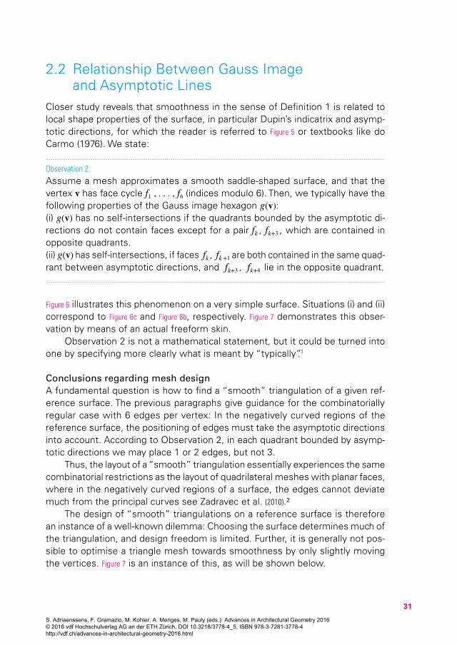