measures of central tendency - kcesmjcollege.in · mean = fd xa n ∑ =+ = 35 – = 35 – 4 = 31....

Measures of Central Tendency:In the study of a population with respect to one in which we

are interested we may get a large number of observations. It is notpossible to grasp any idea about the characteristic when we look atall the observations. So it is better to get one number for one group.That number must be a good representative one for all theobservations to give a clear picture of that characteristic. Suchrepresentative number can be a central value for all theseobservations. This central value is called a measure of centraltendency or an average or a measure of locations. There are fiveaverages. Among them mean, median and mode are called simpleaverages and the other two averages geometric mean and harmonicmean are called special averages.The meaning of average is nicely given in the following definitions.

“A measure of central tendency is a typical value around whichother figures congregate.”“An average stands for the whole group of which it forms a partyet represents the whole.”“One of the most widely used set of summary figures is knownas measures of location.”

Characteristics for a good or an ideal average :The following properties should possess for an ideal average.1. It should be rigidly defined.2. It should be easy to understand and compute.3. It should be based on all items in the data.4. Its definition shall be in the form of a mathematical

formula.5. It should be capable of further algebraic treatment.6. It should have sampling stability.7. It should be capable of being used in further statistical

computations or processing.

MEASURES OF CENTRAL TENDENCY

M.Sc.-Statistics-Chapter-1- PAGE-01

LECTURE NOTES by DR. J.S.V.R. KRISHNA PRASAD

adiani

Typewritten text

MATHEMATICAL STATISTICS; CHAPTER-1

Besides the above requisites, a good average shouldrepresent maximum characteristics of the data, its value should benearest to the most items of the given series.Arithmetic mean or mean :

Arithmetic mean or simply the mean of a variable is definedas the sum of the observations divided by the number ofobservations. If the variable x assumes n values x1, x2 … xn then themean, x, is given by

1 2 3 ....

1

n

n

ii

x x x xxn

xn =1

+ + + +=

= ∑

This formula is for the ungrouped or raw data.

Example 1 :Calculate the mean for 2, 4, 6, 8, 10

Solution:2 4 6 8 10

530 65

x + + + +=

= =

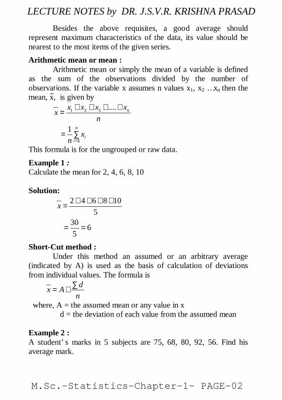
Short-Cut method :Under this method an assumed or an arbitrary average

(indicated by A) is used as the basis of calculation of deviationsfrom individual values. The formula is

dx An

∑= +

where, A = the assumed mean or any value in x d = the deviation of each value from the assumed mean

Example 2 :A student’ s marks in 5 subjects are 75, 68, 80, 92, 56. Find hisaverage mark.



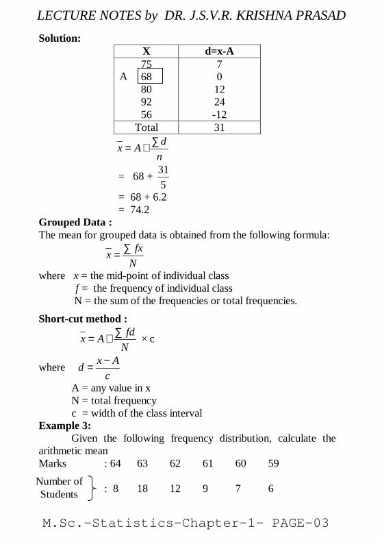
Solution:X d=x-A7568809256

701224-12

Total 31dx A

n∑

= +

= 68 + 315

= 68 + 6.2 = 74.2

Grouped Data :The mean for grouped data is obtained from the following formula:

fxxN

∑=

where x = the mid-point of individual classf = the frequency of individual class

N = the sum of the frequencies or total frequencies.

Short-cut method :fdx A

N∑

= + × c

where x Adc−

=

A = any value in xN = total frequencyc = width of the class interval

Example 3:Given the following frequency distribution, calculate the

arithmetic meanMarks : 64 63 62 61 60 59

: 8 18 12 9 7 6

A

Number ofStudents



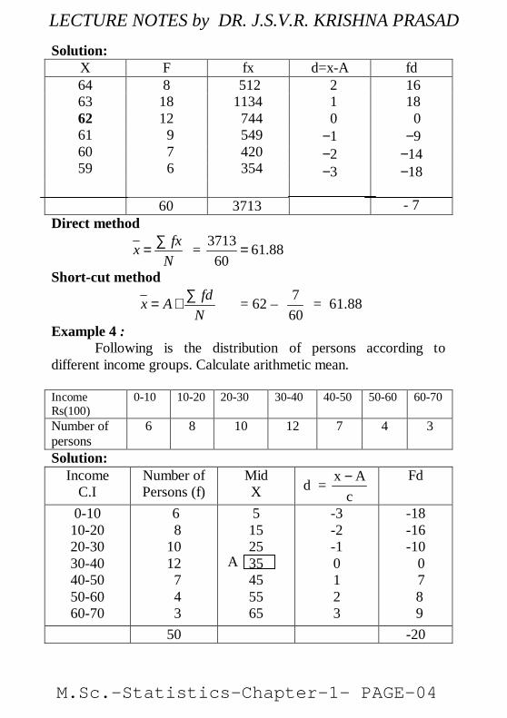
Solution:X F fx d=x-A fd

81812 9 7 6

5121134 744 549 420 354

646362616059

60 3713

2 1 0−1−2−3

16 18 0−9

−14−18

- 7Direct method

fxxN

∑= = 3713 61.88

60=

Short-cut methodfdx A

N∑

= + = 62 – 760

= 61.88

Example 4 :Following is the distribution of persons according to

different income groups. Calculate arithmetic mean.

IncomeRs(100)

0-10 10-20 20-30 30-40 40-50 50-60 60-70

Number ofpersons

6 8 10 12 7 4 3

Solution:Income

C.INumber ofPersons (f)

MidX d =

cAx − Fd

0-1010-2020-3030-4040-5050-6060-70

6 81012 7 4 3

5152535455565

-3-2-10123

-18-16-10 0 7 8 9

50 -20

A



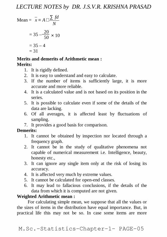
Mean = fdx AN

∑= +

= 35 –

= 35 – 4 = 31Merits and demerits of Arithmetic mean :Merits:

1. It is rigidly defined.2. It is easy to understand and easy to calculate.3. If the number of items is sufficiently large, it is more

accurate and more reliable.4. It is a calculated value and is not based on its position in the

series.5. It is possible to calculate even if some of the details of the

data are lacking.6. Of all averages, it is affected least by fluctuations of

sampling.7. It provides a good basis for comparison.

Demerits:1. It cannot be obtained by inspection nor located through a

frequency graph.2. It cannot be in the study of qualitative phenomena not

capable of numerical measurement i.e. Intelligence, beauty,honesty etc.,

3. It can ignore any single item only at the risk of losing itsaccuracy.

4. It is affected very much by extreme values.5. It cannot be calculated for open-end classes.6. It may lead to fallacious conclusions, if the details of the

data from which it is computed are not given.Weighted Arithmetic mean :

For calculating simple mean, we suppose that all the values orthe sizes of items in the distribution have equal importance. But, inpractical life this may not be so. In case some items are more

20 50 × 10



important than others, a simple average computed is notrepresentative of the distribution. Proper weightage has to be givento the various items. For example, to have an idea of the change incost of living of a certain group of persons, the simple average ofthe prices of the commodities consumed by them will not dobecause all the commodities are not equally important, e.g rice,wheat and pulses are more important than tea, confectionery etc., Itis the weighted arithmetic average which helps in finding out theaverage value of the series after giving proper weight to eachgroup.

Definition:The average whose component items are being multiplied

by certain values known as “weights” and the aggregate of themultiplied results are being divided by the total sum of their“weight”.

If x1, x2…xn be the values of a variable x with respectiveweights of w1, w2… wn assigned to them, then

Weighted A.M = 1 1 2 2

1 2

........

n nw

n

w x w x w xxw w w

+ + +=

+ + + = i i

i

w xw

∑∑

Uses of the weighted mean:Weighted arithmetic mean is used in:

a. Construction of index numbers.b. Comparison of results of two or more universities where

number of students differ.c. Computation of standardized death and birth rates.

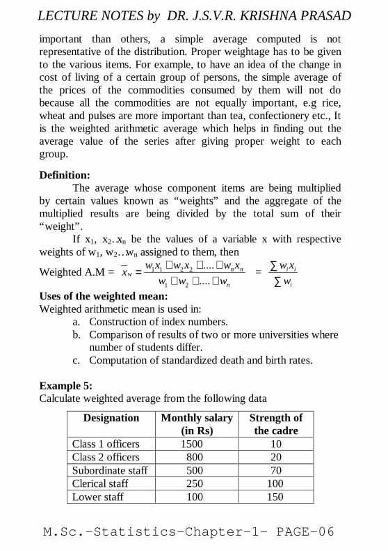
Example 5:Calculate weighted average from the following data

Designation Monthly salary(in Rs)

Strength ofthe cadre

Class 1 officers 1500 10Class 2 officers 800 20Subordinate staff 500 70Clerical staff 250 100Lower staff 100 150



Solution:

Designation Monthlysalary,x

Strength ofthe cadre,w

wx

Class 1 officer 1,500 10 15,000Class 2 officer 800 20 16,000Subordinatestaff

500 70 35,000

Clerical staff 250 100 25,000Lower staff 100 150 15,000

350 1,06,000

Weighted average, wwxxw

∑=

∑

= 106000350

= Rs. 302.86

Harmonic mean (H.M) : Harmonic mean of a set of observations is defined asthe reciprocal of the arithmetic average of the reciprocal of thegiven values. If x1,x2…..xn are n observations,

H.M =n

i 1 i

n1x=

∑For a frequency distribution

=

=

∑. .

n

i i

NHMf

x1

1

Example 6:From the given data calculate H.M 5,10,17,24,30



X 1x

5 0.200010 0.100017 0.058824 0.041730 0.0333

Total 0.4338

H.M =1

n

x ∑

= 50.4338

= 11.526

Example 7: The marks secured by some students of a class are givenbelow. Calculate the harmonic mean.

Marks 20 21 22 23 24 25Number of

Students4 2 7 1 3 1

Solution:

MarksX

No ofstudents

f

1x

ƒ( 1x

)

20 4 0.0500 0.200021 2 0.0476 0.095222 7 0.0454 0.317823 1 0.0435 0.043524 3 0.0417 0.125125 1 0.0400 0.0400

18 0.8216



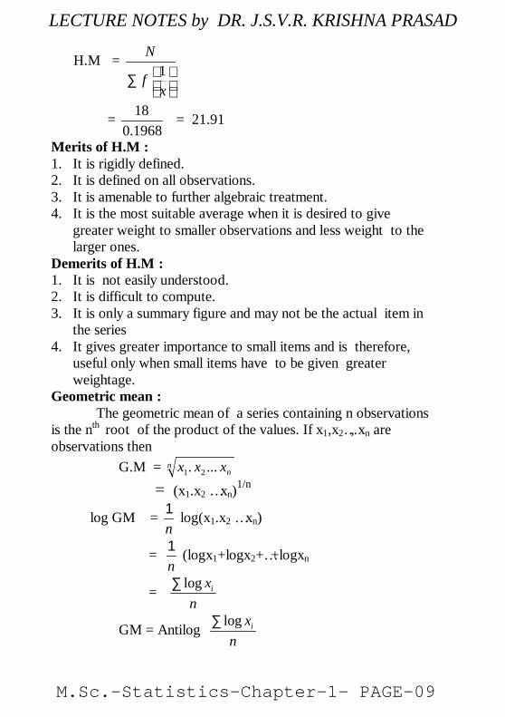
H.M =1

N

fx

∑

=1968.018 = 21.91

Merits of H.M :1. It is rigidly defined.2. It is defined on all observations.3. It is amenable to further algebraic treatment.4. It is the most suitable average when it is desired to give

greater weight to smaller observations and less weight to thelarger ones.

Demerits of H.M :1. It is not easily understood.2. It is difficult to compute.3. It is only a summary figure and may not be the actual item in

the series4. It gives greater importance to small items and is therefore,

useful only when small items have to be given greaterweightage.

Geometric mean : The geometric mean of a series containing n observationsis the nth root of the product of the values. If x1,x2…, xn areobservations then G.M = n

nxxx .... 21

= (x1.x2 … xn)1/n

log GM =n1 log(x1.x2 … xn)

=n1 (logx1+logx2+…+logxn

= log ixn

∑

GM = Antilog log ixn

∑



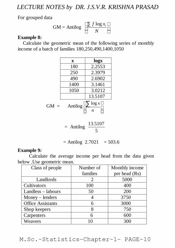
For grouped data

GM = Antiloglog if xN

∑

Example 8: Calculate the geometric mean of the following series of monthlyincome of a batch of families 180,250,490,1400,1050

x logx 180 2.2553 250 2.3979 490 2.6902

1400 3.1461 1050 3.0212

13.5107

GM = Antilog log xn

∑

= Antilog 13.51075

= Antilog 2.7021 = 503.6

Example 9:Calculate the average income per head from the data given

below .Use geometric mean.Class of people Number of

familiesMonthly income

per head (Rs)Landlords 2 5000

Cultivators 100 400Landless – labours 50 200Money – lenders 4 3750Office Assistants 6 3000Shop keepers 8 750Carpenters 6 600Weavers 10 300



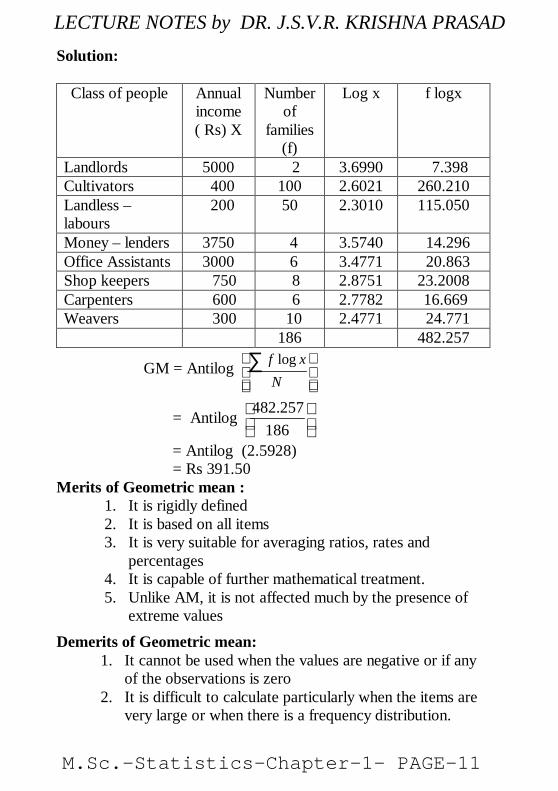
Solution:

Class of people Annualincome( Rs) X

Numberof

families(f)

Log x f logx

Landlords 5000 2 3.6990 7.398Cultivators 400 100 2.6021 260.210Landless –labours

200 50 2.3010 115.050

Money – lenders 3750 4 3.5740 14.296Office Assistants 3000 6 3.4771 20.863Shop keepers 750 8 2.8751 23.2008Carpenters 600 6 2.7782 16.669Weavers 300 10 2.4771 24.771

186 482.257

GM = Antilog logf xN

∑

= Antilog

186257.482

= Antilog (2.5928) = Rs 391.50Merits of Geometric mean :

1. It is rigidly defined2. It is based on all items3. It is very suitable for averaging ratios, rates and

percentages4. It is capable of further mathematical treatment.5. Unlike AM, it is not affected much by the presence of

extreme valuesDemerits of Geometric mean:

1. It cannot be used when the values are negative or if anyof the observations is zero

2. It is difficult to calculate particularly when the items arevery large or when there is a frequency distribution.



105

3. It brings out the property of the ratio of the change andnot the absolute difference of change as the case inarithmetic mean.

4. The GM may not be the actual value of the series.

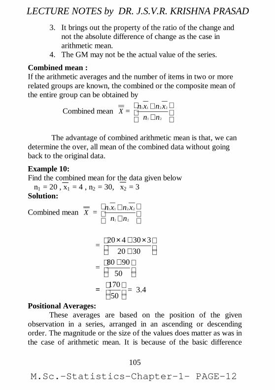
Combined mean :If the arithmetic averages and the number of items in two or morerelated groups are known, the combined or the composite mean ofthe entire group can be obtained by

Combined mean X = 1 1 2 2

1 2

n x n xn n

+ +

The advantage of combined arithmetic mean is that, we candetermine the over, all mean of the combined data without goingback to the original data.

Example 10:Find the combined mean for the data given below n1 = 20 , x1 = 4 , n2 = 30, x2 = 3Solution:

Combined mean X = 1 1 2 2

1 2

n x n xn n

+ +

=20 4 30 3

20 30× + ×

+

=80 90

50+

= 17050

= 3.4

Positional Averages:These averages are based on the position of the given

observation in a series, arranged in an ascending or descendingorder. The magnitude or the size of the values does matter as was inthe case of arithmetic mean. It is because of the basic difference



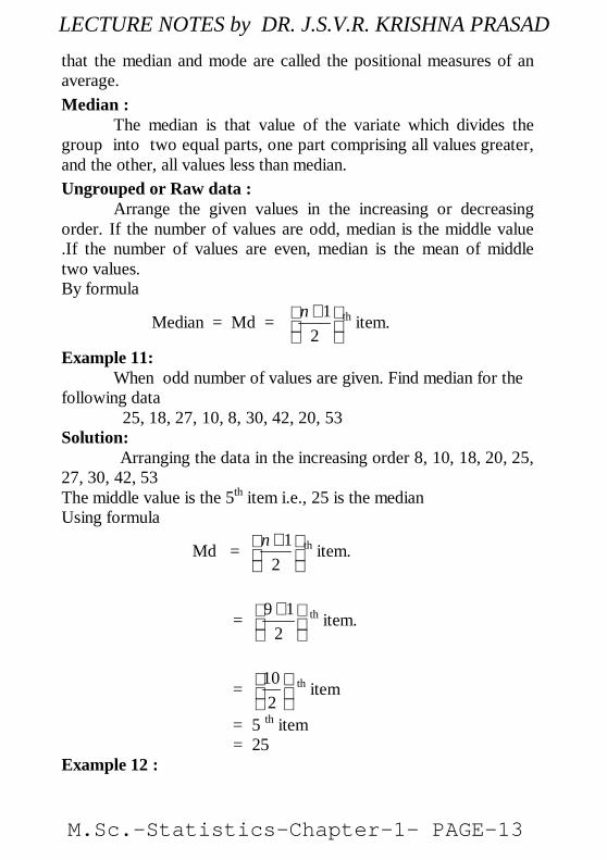
that the median and mode are called the positional measures of anaverage.Median :

The median is that value of the variate which divides thegroup into two equal parts, one part comprising all values greater,and the other, all values less than median.Ungrouped or Raw data :

Arrange the given values in the increasing or decreasingorder. If the number of values are odd, median is the middle value.If the number of values are even, median is the mean of middletwo values.By formula

Median = Md = 12

n +

th item.

Example 11:When odd number of values are given. Find median for the

following data 25, 18, 27, 10, 8, 30, 42, 20, 53

Solution: Arranging the data in the increasing order 8, 10, 18, 20, 25,27, 30, 42, 53The middle value is the 5th item i.e., 25 is the medianUsing formula

Md = 12

n +

th item.

= 9 12+

th item.

= 102

th item

= 5 th item = 25Example 12 :



107

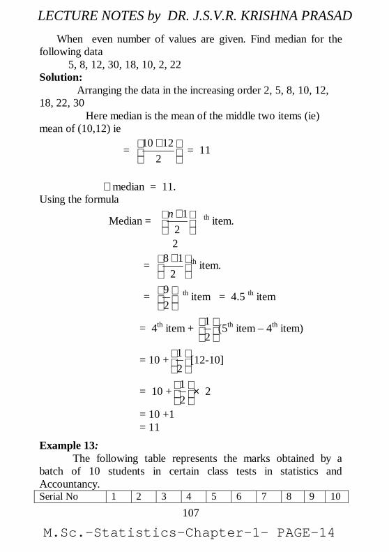
When even number of values are given. Find median for thefollowing data 5, 8, 12, 30, 18, 10, 2, 22Solution: Arranging the data in the increasing order 2, 5, 8, 10, 12,18, 22, 30 Here median is the mean of the middle two items (ie)mean of (10,12) ie

= 10 122+

= 11

∴median = 11.Using the formula

Median = 12

n +

th item.

2

= 8 12+

th item.

= 92

th item = 4.5 th item

= 4th item + 12

(5th item – 4th item)

= 10 + 12

[12-10]

= 10 + 12

× 2

= 10 +1= 11

Example 13:The following table represents the marks obtained by a

batch of 10 students in certain class tests in statistics andAccountancy.Serial No 1 2 3 4 5 6 7 8 9 10



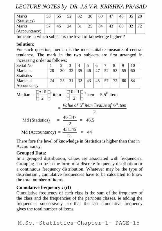
Marks(Statistics)

53 55 52 32 30 60 47 46 35 28

Marks(Accountancy)

57 45 24 31 25 84 43 80 32 72

Indicate in which subject is the level of knowledge higher ?Solution:For such question, median is the most suitable measure of centraltendency. The mark in the two subjects are first arranged inincreasing order as follows:Serial No 1 2 3 4 5 6 7 8 9 10Marks inStatistics

28 30 32 35 46 47 52 53 55 60

Marks inAccountancy

24 25 31 32 43 45 57 72 80 84

Median = 12

n +

th item = 10 12+

th item =5.5th item

= 5 62

th thValue of item value of item+

Md (Statistics) = 46 472+ = 46.5

Md (Accountancy) = 43 452+ = 44

There fore the level of knowledge in Statistics is higher than that inAccountancy.Grouped Data:In a grouped distribution, values are associated with frequencies.Grouping can be in the form of a discrete frequency distribution ora continuous frequency distribution. Whatever may be the type ofdistribution , cumulative frequencies have to be calculated to knowthe total number of items.Cumulative frequency : (cf)Cumulative frequency of each class is the sum of the frequency ofthe class and the frequencies of the pervious classes, ie adding thefrequencies successively, so that the last cumulative frequencygives the total number of items.



Discrete Series:Step1: Find cumulative frequencies.

Step2: Find 12

N +

Step3: See in the cumulative frequencies the value just greater than1

2N +

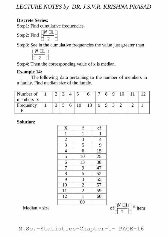
Step4: Then the corresponding value of x is median.Example 14:

The following data pertaining to the number of members ina family. Find median size of the family.

Number ofmembers x

1 2 3 4 5 6 7 8 9 10 11 12

Frequency F

1 3 5 6 10 13 9 5 3 2 2 1

Solution:

Median = size of 12

N +

th item

X f cf1 1 12 3 43 5 94 6 155 10 256 13 387 9 478 5 529 3 55

10 2 57 11 2 59 12 1 60

60



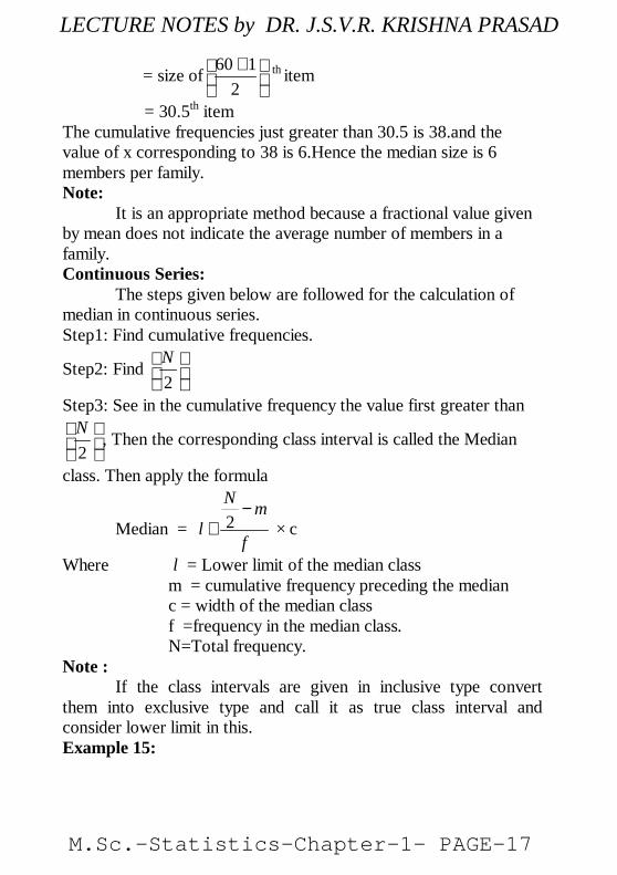
= size of 60 12+

th item

= 30.5th itemThe cumulative frequencies just greater than 30.5 is 38.and thevalue of x corresponding to 38 is 6.Hence the median size is 6members per family.Note:

It is an appropriate method because a fractional value givenby mean does not indicate the average number of members in afamily.Continuous Series:

The steps given below are followed for the calculation ofmedian in continuous series.Step1: Find cumulative frequencies.

Step2: Find2N

Step3: See in the cumulative frequency the value first greater than

2N

, Then the corresponding class interval is called the Median

class. Then apply the formula

Median = 2N m

lf

−+ × c

Where l = Lower limit of the median classm = cumulative frequency preceding the medianc = width of the median classf =frequency in the median class.N=Total frequency.

Note :If the class intervals are given in inclusive type convert

them into exclusive type and call it as true class interval andconsider lower limit in this.Example 15:



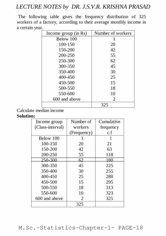
The following table gives the frequency distribution of 325workers of a factory, according to their average monthly income ina certain year.

Income group (in Rs) Number of workersBelow 100100-150150-200200-250250-300300-350350-400400-450450-500500-550550-600

600 and above

120425562453025151810 2

325Calculate median incomeSolution:

Income group(Class-interval)

Number ofworkers

(Frequency)

Cumulativefrequency

c.fBelow 100100-150150-200200-250250-300300-350350-400400-450450-500500-550550-600

600 and above

120425562453025151810 2

12163118180225255280295313323325

325



3252 2N

= =162.5

Here l = 250, N = 325, f = 62, c = 50, m = 118

Md = 250+ 162.5 11862

−

× 50

= 250+35.89 = 285.89

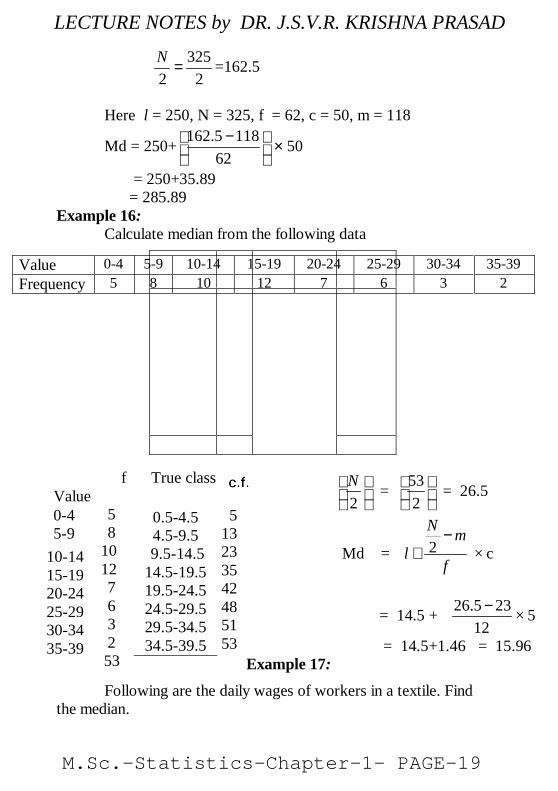
Example 16:Calculate median from the following data

2N

= 532

= 26.5

Md = 2N m

lf

−+ × c

= 14.5 + 26.5 2312

− × 5

= 14.5+1.46 = 15.96Example 17:

Following are the daily wages of workers in a textile. Findthe median.

Value 0-4 5-9 10-14 15-19 20-24 25-29 30-34 35-39Frequency 5 8 10 12 7 6 3 2

Valuef True class

0-4 5-910-1415-1920-2425-2930-3435-39

58

10127632

0.5-4.54.5-9.5

9.5-14.514.5-19.519.5-24.524.5-29.529.5-34.534.5-39.5

513233542485153

53



adiani

Typewritten text

c.f.

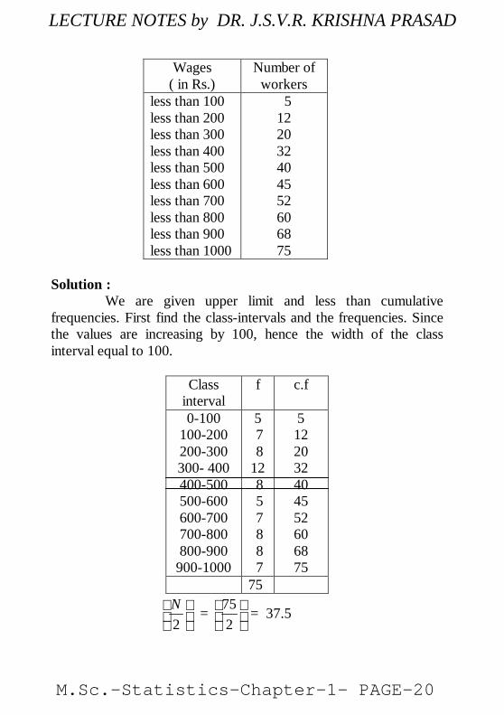
Wages( in Rs.)

Number ofworkers

less than 100less than 200less than 300less than 400less than 500less than 600less than 700less than 800less than 900less than 1000

5122032404552606875

Solution :We are given upper limit and less than cumulative

frequencies. First find the class-intervals and the frequencies. Sincethe values are increasing by 100, hence the width of the classinterval equal to 100.

Classinterval

f c.f

0-100100-200200-300300- 400400-500500-600600-700700-800800-900

900-1000

5 7 812 8 5 7 8 8 7

5122032404552606875

75

2N

= 752

= 37.5



Md = l + 2N m

f

−

× c

= 400 + 37.5 328−

× 100 = 400 + 68.75 = 468.75

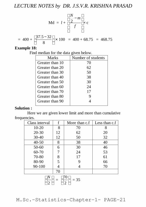
Example 18: Find median for the data given below.

Marks Number of studentsGreater than 10Greater than 20Greater than 30Greater than 40Greater than 50Greater than 60Greater than 70Greater than 80Greater than 90

70625038302417 9 4

Solution :Here we are given lower limit and more than cumulative

frequencies.Class interval f More than c.f Less than c.f

10-2020-3030-40

8 12 12

706250

82032

40-50 8 38 4050-6060-7070-8080-90

90-100

67854

302417 9 4

4653616670

70

2N

= 702

= 35



Median = l + 2N m

xcf

−

= 40 + 35 328−

× 10

= 40 +3.75 = 43.75

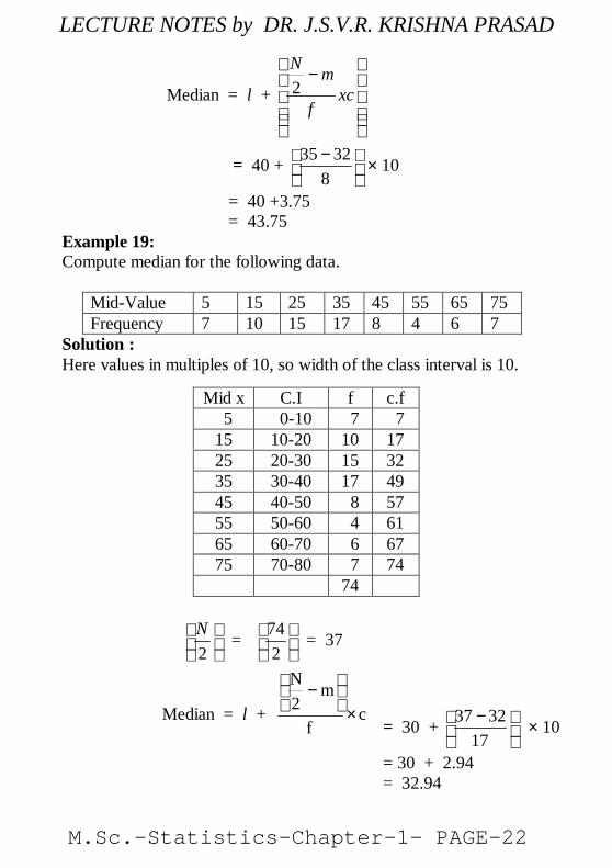
Example 19:Compute median for the following data.

Mid-Value 5 15 25 35 45 55 65 75Frequency 7 10 15 17 8 4 6 7

Solution :Here values in multiples of 10, so width of the class interval is 10.

2N

= 742

= 37

Median = l + cf

m2N

×

−

Mid x C.I f c.f 5 0-10 7 715 10-20 10 1725 20-30 15 3235 30-40 17 4945 40-50 8 5755 50-60 4 6165 60-70 6 6775 70-80 7 74

74

= 30 + 37 3217−

× 10

= 30 + 2.94 = 32.94



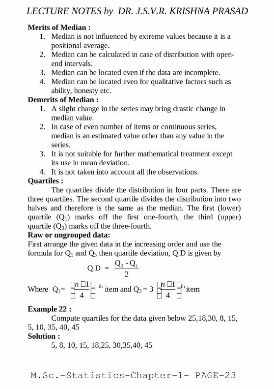
Merits of Median :1. Median is not influenced by extreme values because it is a

positional average.2. Median can be calculated in case of distribution with open-

end intervals.3. Median can be located even if the data are incomplete.4. Median can be located even for qualitative factors such as

ability, honesty etc.Demerits of Median :

1. A slight change in the series may bring drastic change inmedian value.

2. In case of even number of items or continuous series,median is an estimated value other than any value in theseries.

3. It is not suitable for further mathematical treatment exceptits use in mean deviation.

4. It is not taken into account all the observations.Quartiles :

The quartiles divide the distribution in four parts. There arethree quartiles. The second quartile divides the distribution into twohalves and therefore is the same as the median. The first (lower)quartile (Q1) marks off the first one-fourth, the third (upper)quartile (Q3) marks off the three-fourth.Raw or ungrouped data:First arrange the given data in the increasing order and use theformula for Q1 and Q3 then quartile deviation, Q.D is given by

Q.D =2

Q-Q 13

Where Q1=1

4n +

th item and Q3 = 3 14

n +

th item

Example 22 :Compute quartiles for the data given below 25,18,30, 8, 15,

5, 10, 35, 40, 45Solution :

5, 8, 10, 15, 18,25, 30,35,40, 45



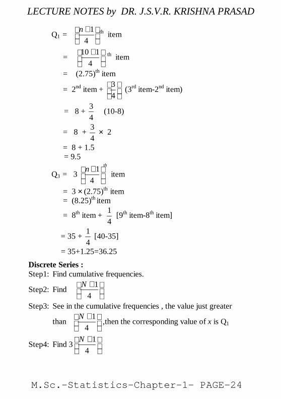
Q1 = 14

n +

th item

= 10 14+

th item

= (2.75)th item

= 2nd item + 34

(3rd item-2nd item)

= 8 + 34

(10-8)

= 8 + 34

× 2

= 8 + 1.5 = 9.5

Q3 = 3 14

thn +

item

= 3 × (2.75)th item = (8.25)th item

= 8th item + 14

[9th item-8th item]

= 35 + 14

[40-35]

= 35+1.25=36.25Discrete Series :Step1: Find cumulative frequencies.

Step2: Find 14

N +

Step3: See in the cumulative frequencies , the value just greater

than 14

N +

,then the corresponding value of x is Q1

Step4: Find 3 14

N +



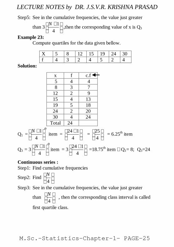
Step5: See in the cumulative frequencies, the value just greater

than 3 14

N +

,then the corresponding value of x is Q3

Example 23:Compute quartiles for the data given bellow.

Solution:

Q1 = 14

thN +

item = 24 14+

= 254

= 6.25th item

Q3 = 3 14

thN +

item = 3 24 14+

=18.75th item ∴Q1= 8; Q3=24

Continuous series :Step1: Find cumulative frequencies

Step2: Find4N

Step3: See in the cumulative frequencies, the value just greater

than4N

, then the corresponding class interval is called

first quartile class.

X 5 8 12 15 19 24 30f 4 3 2 4 5 2 4

x f c.f 5 4 4 8 3 712 2 915 4 1319 5 1824 2 2030 4 24

Total 24



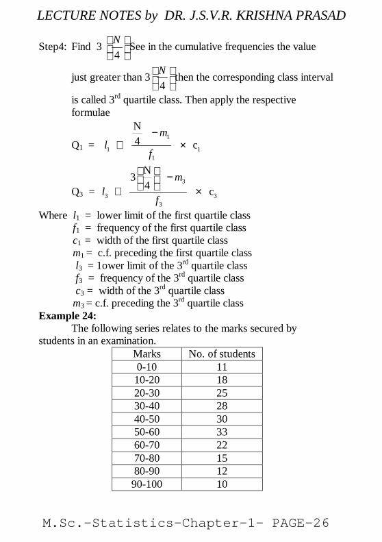
Step4: Find 34

N See in the cumulative frequencies the value

just greater than 34

N then the corresponding class interval

is called 3rd quartile class. Then apply the respectiveformulae

Q1 =1

1 11

N4 c

ml

f

−+ ×

Q3 =3

3 33

N34 c

ml

f

− + ×

Where l1 = lower limit of the first quartile class f1 = frequency of the first quartile class c1 = width of the first quartile class m1 = c.f. preceding the first quartile class l3 = 1ower limit of the 3rd quartile class f3 = frequency of the 3rd quartile class c3 = width of the 3rd quartile class m3 = c.f. preceding the 3rd quartile classExample 24:

The following series relates to the marks secured bystudents in an examination.

Marks No. of students0-10 1110-20 1820-30 2530-40 2840-50 3050-60 3360-70 2270-80 1580-90 12

90-100 10



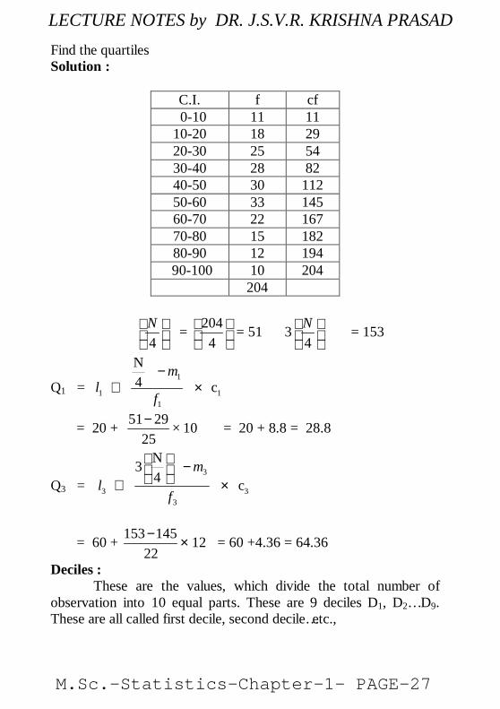
Find the quartilesSolution :

C.I. f cf 0-10 11 1110-20 18 2920-30 25 5430-40 28 8240-50 30 11250-60 33 14560-70 22 16770-80 15 18280-90 12 194

90-100 10 204204

4N

= 2044

= 51 34N

= 153

Q1 =1

1 11

N4 c

ml

f

−+ ×

= 20 + 51 2925− × 10 = 20 + 8.8 = 28.8

Q3 =3

3 33

N34 c

ml

f

− + ×

= 60 + 153 14522−

× 12 = 60 +4.36 = 64.36

Deciles :These are the values, which divide the total number of

observation into 10 equal parts. These are 9 deciles D1, D2… D9.These are all called first decile, second decile…etc.,



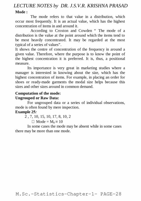
Mode :The mode refers to that value in a distribution, which

occur most frequently. It is an actual value, which has the highestconcentration of items in and around it.

According to Croxton and Cowden “ The mode of adistribution is the value at the point around which the items tend tobe most heavily concentrated. It may be regarded at the mosttypical of a series of values”.It shows the centre of concentration of the frequency in around agiven value. Therefore, where the purpose is to know the point ofthe highest concentration it is preferred. It is, thus, a positionalmeasure.

Its importance is very great in marketing studies where amanager is interested in knowing about the size, which has thehighest concentration of items. For example, in placing an order forshoes or ready-made garments the modal size helps because thissizes and other sizes around in common demand.

Computation of the mode:Ungrouped or Raw Data:

∴ Mode = M0 =10In some cases the mode may be absent while in some cases

there may be more than one mode.

For ungrouped data or a series of individual observations,mode is often found by mere inspection.Example 25: 2 , 7, 10, 15, 10, 17, 8, 10, 2



129

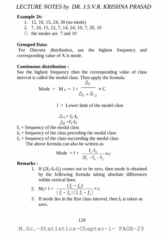
Grouped Data:For Discrete distribution, see the highest frequency and

corresponding value of X is mode.

Continuous distribution :See the highest frequency then the corresponding value of classinterval is called the modal class. Then apply the formula.

1

Mode = M 0 = l + × C1 + 2

l = Lower limit of the model class

1 = f1-f0

2 =f1-f2f1 = frequency of the modal classf0 = frequency of the class preceding the modal classf2 = frequency of the class succeeding the modal class The above formula can also be written as

Mode = l + 1 0

1 0 2

f -f2f - f - f

c×

Remarks :1. If (2f1-f0-f2) comes out to be zero, then mode is obtained

by the following formula taking absolute differenceswithin vertical lines.

2. M0= l + 1 0

1 0 1 2

( )| | | |

f ff f f f

−− + −

× c

3. If mode lies in the first class interval, then f0 is taken aszero.

Example 26:1. 12, 10, 15, 24, 30 (no mode)2. 7, 10, 15, 12, 7, 14, 24, 10, 7, 20, 10∴ the modes are 7 and 10



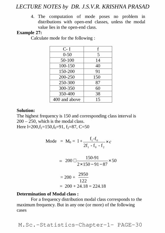
4. The computation of mode poses no problem indistributions with open-end classes, unless the modalvalue lies in the open-end class.

C- I f 0-50 5

50-100 14100-150 40150-200 91200-250 150250-300 87300-350 60350-400 38

400 and above 15

Solution:The highest frequency is 150 and corresponding class interval is200 – 250, which is the modal class.Here l=200,f1=150,f0=91, f2=87, C=50

Mode = M0 = l + 1 0

1 0 2

f -f2f - f - f

c×

=150-91200 50

2 150 91 87+ ×

× − −

= 200 + 2950122

= 200 + 24.18 = 224.18

Determination of Modal class :For a frequency distribution modal class corresponds to the

maximum frequency. But in any one (or more) of the followingcases

Example 27:Calculate mode for the following :



131

i.If the maximum frequency is repeatedii.If the maximum frequency occurs in the beginning or at the

end of the distributioniii.If there are irregularities in the distribution, the modal class

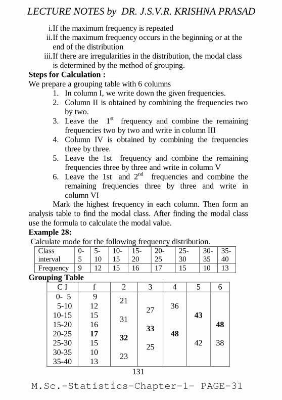
is determined by the method of grouping.Steps for Calculation :We prepare a grouping table with 6 columns

1. In column I, we write down the given frequencies.2. Column II is obtained by combining the frequencies two

by two.3. Leave the 1st frequency and combine the remaining

frequencies two by two and write in column III4. Column IV is obtained by combining the frequencies

three by three.5. Leave the 1st frequency and combine the remaining

frequencies three by three and write in column V6. Leave the 1st and 2nd frequencies and combine the

remaining frequencies three by three and write incolumn VI

Classinterval

0-5

5-10

10-15

15-20

20-25

25-30

30-35

35-40

Frequency 9 12 15 16 17 15 10 13Grouping Table

C I f 2 3 4 5 6 0- 5 5-1010-1515-2020-2525-3030-3535-40

912151617151013

21

31

32

23

27

33

25

36

48

43

42

48

38

Mark the highest frequency in each column. Then form ananalysis table to find the modal class. After finding the modal classuse the formula to calculate the modal value.Example 28: Calculate mode for the following frequency distribution.



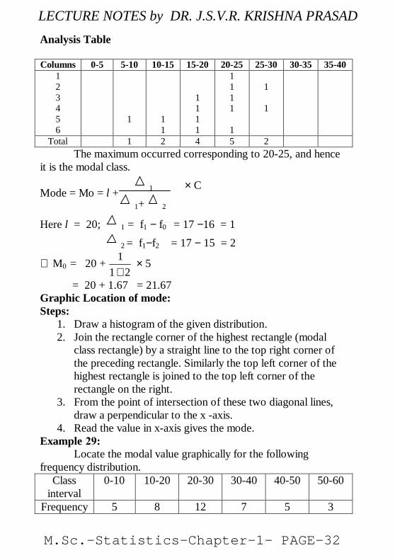
Analysis Table

Columns 0-5 5-10 10-15 15-20 20-25 25-30 30-35 35-40123456

1 11

1111

1111

1

1

1

Total 1 2 4 5 2The maximum occurred corresponding to 20-25, and hence

it is the modal class.

Mode = Mo = l +

Here l = 20; 1 = f1 − f0 = 17 −16 = 1

2 = f1−f2 = 17 − 15 = 2

∴ M0 = 20 +21

1+

× 5

= 20 + 1.67 = 21.67Graphic Location of mode:Steps:

1. Draw a histogram of the given distribution.2. Join the rectangle corner of the highest rectangle (modal

class rectangle) by a straight line to the top right corner ofthe preceding rectangle. Similarly the top left corner of thehighest rectangle is joined to the top left corner of therectangle on the right.

3. From the point of intersection of these two diagonal lines,draw a perpendicular to the x -axis.

Locate the modal value graphically for the followingfrequency distribution.

Classinterval

0-10 10-20 20-30 30-40 40-50 50-60

Frequency 5 8 12 7 5 3

1 × C

1+ 2

4. Read the value in x-axis gives the mode.Example 29:



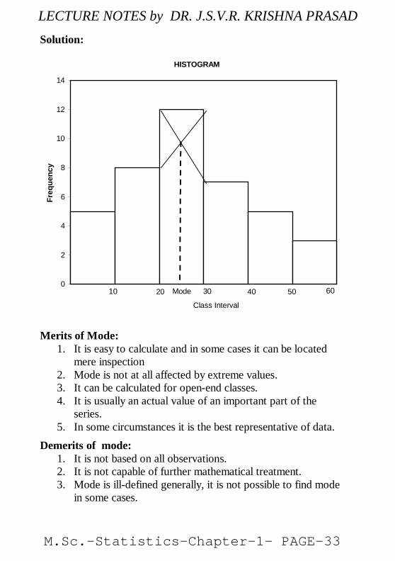
Solution:

HISTOGRAM

0

2

4

6

8

10

12

14

Daily Wages (in Rs.)

Freq

uenc

y

10 30 40 50 60 20

Class Interval

Mode

Merits of Mode:1. It is easy to calculate and in some cases it can be located

mere inspection2. Mode is not at all affected by extreme values.3. It can be calculated for open-end classes.4. It is usually an actual value of an important part of the

series.5. In some circumstances it is the best representative of data.

Demerits of mode:1. It is not based on all observations.2. It is not capable of further mathematical treatment.3. Mode is ill-defined generally, it is not possible to find mode

in some cases.



4. As compared with mean, mode is affected to a great extent,by sampling fluctuations.

5. It is unsuitable in cases where relative importance of itemshas to be considered.

EMPIRICAL RELATIONSHIP BETWEEN AVERAGESIn a symmetrical distribution the three simple averages

mean = median = mode. For a moderately asymmetricaldistribution, the relationship between them are brought by Prof.Karl Pearson as mode = 3median - 2mean.Example 34:

If the mean and median of a moderately asymmetrical seriesare 26.8 and 27.9 respectively, what would be its most probablemode?Solution:

Using the empirical formulaMode = 3 median − 2 mean = 3 × 27.9 − 2 × 26.8 = 30.1

mode and mean are 32.1 and 35.4 respectively. Find the medianvalue.Solution:

Using empirical Formula

Median =31 [2mean+mode]

=31 [2 × 35.4 + 32.1]

= 34.3

Example 30:In a moderately asymmetrical distribution the values of



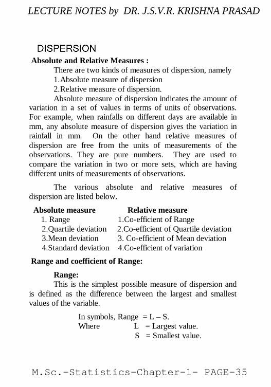
variation in a set of values in terms of units of observations.For example, when rainfalls on different days are available inmm, any absolute measure of dispersion gives the variation inrainfall in mm. On the other hand relative measures ofdispersion are free from the units of measurements of theobservations. They are pure numbers. They are used tocompare the variation in two or more sets, which are havingdifferent units of measurements of observations.

The various absolute and relative measures ofdispersion are listed below.

Absolute measure Relative measure 1. Range 1.Co-efficient of Range

2.Quartile deviation 2.Co-efficient of Quartile deviation 3.Mean deviation 3. Co-efficient of Mean deviation 4.Standard deviation 4.Co-efficient of variation

is defined as the difference between the largest and smallestvalues of the variable.

In symbols, Range = L – S.Where L = Largest value.

S = Smallest value.

Absolute and Relative Measures :There are two kinds of measures of dispersion, namely1.Absolute measure of dispersion2.Relative measure of dispersion.Absolute measure of dispersion indicates the amount of

Range and coefficient of Range:

Range:This is the simplest possible measure of dispersion and



adiani

Typewritten text

DISPERSION

143

In individual observations and discrete series, L and Sare easily identified. In continuous series, the following twomethods are followed.Method 1:

L = Upper boundary of the highest class S = Lower boundary of the lowest class.

Method 2: L = Mid value of the highest class. S = Mid value of the lowest class.

SLSL

+−

Example1:Find the value of range and its co-efficient for the followingdata.

7, 9, 6, 8, 11, 10, 4Solution:L=11, S = 4.Range = L – S = 11- 4 = 7

Co-efficient of Range =SLSL

+−

=411411

+−

=157 = 0.4667

Example 2:Calculate range and its co efficient from the followingdistribution.

Size: 60-63 63-66 66-69 69-72 72-75Number: 5 18 42 27 8

Solution:L = Upper boundary of the highest class. = 75

Co-efficient of Range :

Co-efficient of Range =



144

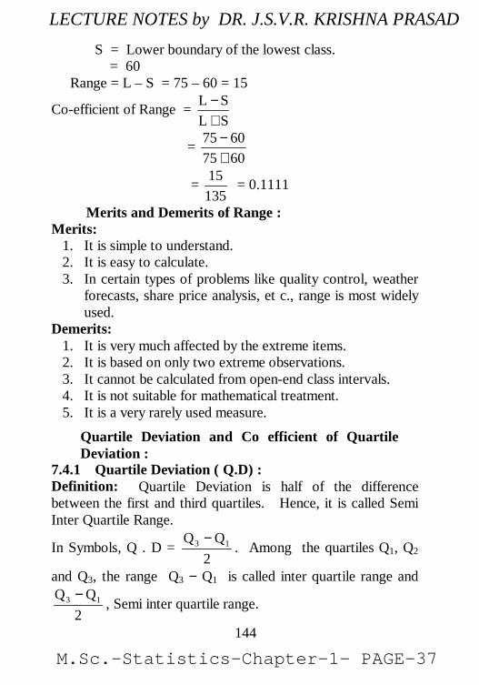
S = Lower boundary of the lowest class. = 60

Range = L – S = 75 – 60 = 15

Co-efficient of Range =SLSL

+−

=60756075

+−

=13515 = 0.1111

1. It is simple to understand.2. It is easy to calculate.3. In certain types of problems like quality control, weather

forecasts, share price analysis, et c., range is most widelyused.

Demerits:1. It is very much affected by the extreme items.2. It is based on only two extreme observations.3. It cannot be calculated from open-end class intervals.4. It is not suitable for mathematical treatment.5. It is a very rarely used measure.

7.4.1 Quartile Deviation ( Q.D) :Definition: Quartile Deviation is half of the differencebetween the first and third quartiles. Hence, it is called SemiInter Quartile Range.

In Symbols, Q . D =2

QQ 13 − . Among the quartiles Q1, Q2

and Q3, the range Q3 − Q1 is called inter quartile range and

2QQ 13 − , Semi inter quartile range.

Merits and Demerits of Range :Merits:

Quartile Deviation and Co efficient of QuartileDeviation :



145

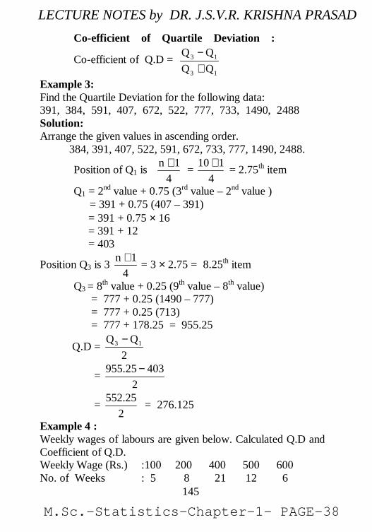
13

13

QQQQ

+−

Example 3:Find the Quartile Deviation for the following data:391, 384, 591, 407, 672, 522, 777, 733, 1490, 2488Solution:Arrange the given values in ascending order. 384, 391, 407, 522, 591, 672, 733, 777, 1490, 2488.

Position of Q1 is 41n + =

4110 + = 2.75th item

Q1 = 2nd value + 0.75 (3rd value – 2nd value ) = 391 + 0.75 (407 – 391)

= 391 + 0.75 × 16 = 391 + 12 = 403

Position Q3 is 34

1n + = 3 × 2.75 = 8.25th item

Q3 = 8th value + 0.25 (9th value – 8th value) = 777 + 0.25 (1490 – 777) = 777 + 0.25 (713) = 777 + 178.25 = 955.25

Q.D =2

QQ 13 −

=2

40325.955 −

= 552.252

= 276.125

Example 4 :Weekly wages of labours are given below. Calculated Q.D andCoefficient of Q.D.Weekly Wage (Rs.) :100 200 400 500 600No. of Weeks : 5 8 21 12 6

Co-efficient of Quartile Deviation :

Co-efficient of Q.D =



146

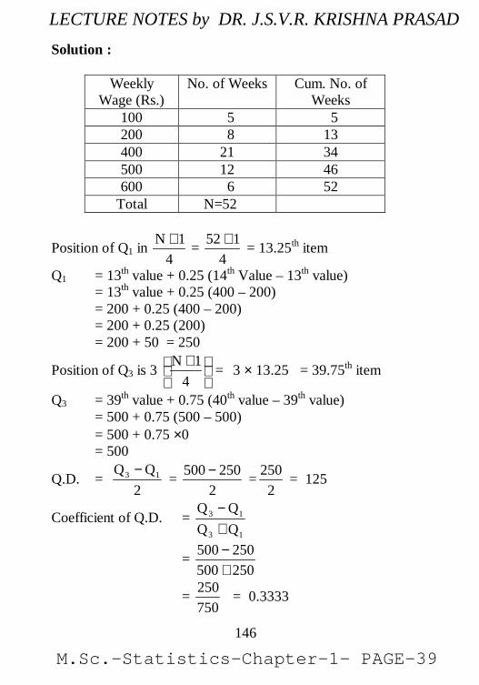
Solution :

WeeklyWage (Rs.)

No. of Weeks Cum. No. ofWeeks

100 5 5200 8 13400 21 34500 12 46600 6 52

Total N=52

Position of Q1 in 41N + =

4152 + = 13.25th item

Q1 = 13th value + 0.25 (14th Value – 13th value)= 13th value + 0.25 (400 – 200)= 200 + 0.25 (400 – 200)= 200 + 0.25 (200)= 200 + 50 = 250

Position of Q3 is 3

+

41N = 3 × 13.25 = 39.75th item

Q3 = 39th value + 0.75 (40th value – 39th value)= 500 + 0.75 (500 – 500)= 500 + 0.75 ×0= 500

Q.D. =2

QQ 13 − =2

250500 − =2

250 = 125

Coefficient of Q.D. =13

13

QQQQ

+−

=250500250500

+−

=750250 = 0.3333



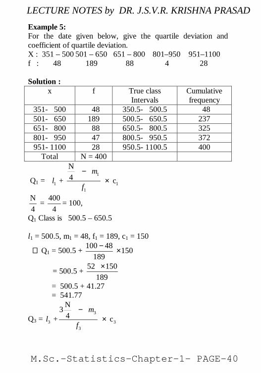
Example 5:For the date given below, give the quartile deviation andcoefficient of quartile deviation.X : 351 – 500 501 – 650 651 – 800 801–950 951–1100f : 48 189 88 4 28

Solution :x f True class

IntervalsCumulativefrequency

351- 500 48 350.5- 500.5 48501- 650 189 500.5- 650.5 237651- 800 88 650.5- 800.5 325801- 950 47 800.5- 950.5 372951- 1100 28 950.5- 1100.5 400

Total N = 400

Q1 =1

1 11

N4 + c

ml

f

−×

4N =

4400 = 100,

Q1 Class is 500.5 – 650.5

l1 = 500.5, m1 = 48, f1 = 189, c1 = 150

∴∴ Q1 = 500.5 + 150189

48100×

−

= 500.5 + 52 150189

×

= 500.5 + 41.27= 541.77

Q3 =3

3 33

N34 + c

ml

f

−×



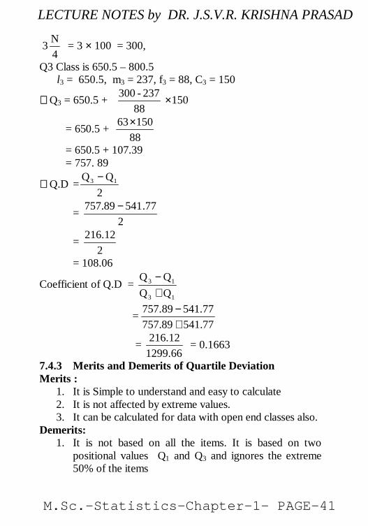
34N = 3 × 100 = 300,

Q3 Class is 650.5 – 800.5 l3 = 650.5, m3 = 237, f3 = 88, C3 = 150

∴∴Q3 = 650.5 + 15088

237-300×

= 650.5 +88

15063×

= 650.5 + 107.39 = 757. 89

∴∴Q.D =2

QQ 13 −

=2

.7754189.757 −

=2

12.216

= 108.06

Coefficient of Q.D =13

13

QQQQ

+−

=77.54189.75777.54189.757

+−

=66.129912.216 = 0.1663

7.4.3 Merits and Demerits of Quartile DeviationMerits :

1. It is Simple to understand and easy to calculate2. It is not affected by extreme values.3. It can be calculated for data with open end classes also.

Demerits:1. It is not based on all the items. It is based on two

positional values Q1 and Q3 and ignores the extreme50% of the items



2. It is not amenable to further mathematical treatment.3. It is affected by sampling fluctuations.

The range and quartile deviation are not based on allobservations. They are positional measures of dispersion. Theydo not show any scatter of the observations from an average.The mean deviation is measure of dispersion based on allitems in a distribution.Definition:

Mean deviation is the arithmetic mean of the deviationsof a series computed from any measure of central tendency;i.e., the mean, median or mode, all the deviations are taken aspositive i.e., signs are ignored. According to Clark andSchekade,

“Average deviation is the average amount scatter of theitems in a distribution from either the mean or the median,ignoring the signs of the deviations”.

We usually compute mean deviation about any one ofthe three averages mean, median or mode. Some times modemay be ill defined and as such mean deviation is computedfrom mean and median. Median is preferred as a choicebetween mean and median. But in general practice and due towide applications of mean, the mean deviation is generallycomputed from mean. M.D can be used to denote meandeviation.

tendency is an absolute measure. For the purpose of comparingvariation among different series, a relative mean deviation isrequired. The relative mean deviation is obtained by dividingthe mean deviation by the average used for calculating meandeviation.

Mean Deviation and Coefficient of Mean Deviation:Mean Deviation:

Coefficient of mean deviation:Mean deviation calculated by any measure of central



Coefficient of mean deviation: = Mean deviationMean or Median or Mode

If the result is desired in percentage, the coefficient of mean

deviation = Mean deviationMean or Median or Mode

× 100

series.2. Take the deviations of items from average ignoring

signs and denote these deviations by |D|.3. Compute the total of these deviations, i.e., Σ |D|4. Divide this total obtained by the number of items.

Symbolically: M.D. = |D|n

∑

Example 6:Calculate mean deviation from mean and median for thefollowing data:100,150,200,250,360,490,500,600,671 also calculate co-efficients of M.D.

Solution:

Mean = x =n

x∑ =9

3321 =369

Now arrange the data in ascending order100, 150, 200, 250, 360, 490, 500, 600, 671

Median = Value of item2

1n th

+

= Value of item2

19 th

+

= Value of 5th item= 360

Computation of mean deviation – Individual Series :1.Calculate the average mean, median or mode of the



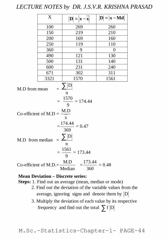
X xxD −= MdxD −=

100 269 260150 219 210200 169 160250 119 110360 9 0490 121 130500 131 140600 231 240671 302 311

3321 1570 1561

M.D from mean =D

n∑

=9

1570 = 174.44

Co-efficient of M.D =x

M.D

=369

44.174 = 0.47

M.D from median =D

n∑

=9

1561 = 173.44

Co-efficient of M.D.= M.DMedian

=360

44.173 = 0.48

2. Find out the deviation of the variable values from the average, ignoring signs and denote them by D3. Multiply the deviation of each value by its respective frequency and find out the total f D∑

Mean Deviation – Discrete series: Steps: 1. Find out an average (mean, median or mode)



4. Divide f D∑ by the total frequencies N

Symbolically, M.D. =f DN

∑

Example 7:Compute Mean deviation from mean and median from the

following data:Heightin cms

158 159 160 161 162 163 164 165 166

No. ofpersons

15 20 32 35 33 22 20 10 8

Also compute coefficient of mean deviation.

Solution:Height

XNo. ofpersons

f

d= x- AA =162 fd

|D| =|X- mean|

f|D|

158 15 - 4 - 60 3.51 52.65159 20 - 3 - 60 2.51 50.20160 32 - 2 - 64 1.51 48.32161 35 - 1 - 35 0.51 17.85162 33 0 0 0.49 16.17163 22 1 22 1.49 32.78164 20 2 40 2.49 49.80165 10 3 30 3.49 34.90166 8 4 32 4.49 35.92

195 - 95 338.59

x =fd

AN

+ ∑

=195

95162 −+ = 162 – 0.49 = 161.51

M.D. =f DN

∑ =195

59.338 = 1.74



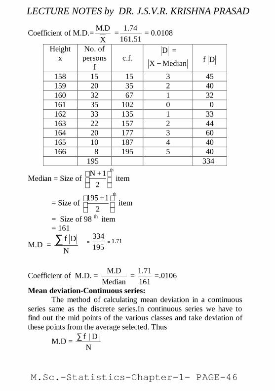
Coefficient of M.D.= M.DX

=51.161

74.1 = 0.0108

Heightx

No. ofpersons

fc.f.

D =

X Median− f D

158 15 15 3 45159 20 35 2 40160 32 67 1 32161 35 102 0 0162 33 135 1 33163 22 157 2 44164 20 177 3 60165 10 187 4 40166 8 195 5 40

195 334

Median = Size ofthN +1 item

2

= Size ofth195 +1 item

2

= Size of 98 th item= 161

M.D =f DN

∑ =195334

= 1.71

Coefficient of M.D. = M.DMedian

=161

71.1 =.0106

series same as the discrete series.In continuous series we have tofind out the mid points of the various classes and take deviation ofthese points from the average selected. Thus

M.D =N

|D|f∑

Mean deviation-Continuous series:The method of calculating mean deviation in a continuous



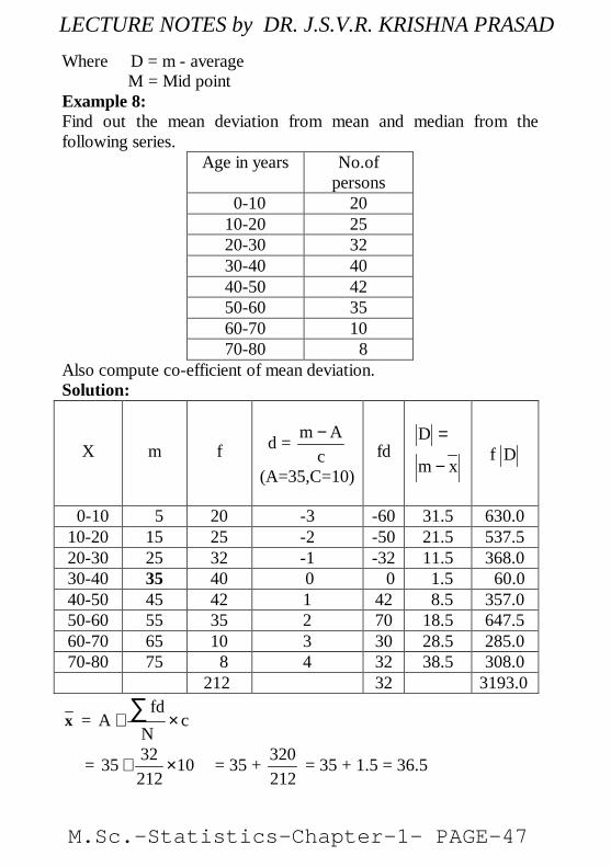
Where D = m - average M = Mid point

Example 8:Find out the mean deviation from mean and median from thefollowing series.

Age in years No.ofpersons

0-10 2010-20 2520-30 3230-40 4040-50 4250-60 3560-70 1070-80 8

Also compute co-efficient of mean deviation.Solution:

X m f d = m Ac−

(A=35,C=10)fd

D

m x

=

−f D

0-10 5 20 -3 -60 31.5 630.010-20 15 25 -2 -50 21.5 537.520-30 25 32 -1 -32 11.5 368.030-40 35 40 0 0 1.5 60.040-50 45 42 1 42 8.5 357.050-60 55 35 2 70 18.5 647.560-70 65 10 3 30 28.5 285.070-80 75 8 4 32 38.5 308.0

212 32 3193.0

x =fd

A cN

+ ×∑

= 3235 10212

+ × = 35 +212320 = 35 + 1.5 = 36.5



M.D. =f DN

∑ =212

3193 = 15.06

Calculation of median and M.D. from median

X m f c.f |D| = |m-Md| f |D|

0-10 5 20 20 32.25 645.0010-20 15 25 45 22.25 556.2520-30 25 32 77 12.25 392.0030-40 35 40 117 2.25 90.0040-50 45 42 159 7.75 325.5050-60 55 35 194 17.75 621.2560-70 65 10 204 27.75 277.5070-80 75 8 212 37.75 302.00

Total 3209.50

2N = 212

2 = 106

l = 30, m = 77, f = 40, c = 10

Median =

N2 + c

ml

f

−×

= 30 +40

77-106× 10

= 30 +429

= 30 + 7.25 = 37.25

M. D. =N

|D|f∑

=212

3209.5 = 15.14

Coefficient of M.D =Median

D.M

=25.3714.15 = 0.41



1. It is simple to understand and easy to compute.2. It is rigidly defined.3. It is based on all items of the series.4. It is not much affected by the fluctuations of sampling.5. It is less affected by the extreme items.6. It is flexible, because it can be calculated from any average.7. It is better measure of comparison.

Demerits:1. It is not a very accurate measure of dispersion.2. It is not suitable for further mathematical calculation.3. It is rarely used. It is not as popular as standard deviation.4. Algebraic positive and negative signs are ignored. It is

mathematically unsound and illogical.

Karl Pearson introduced the concept of standard deviationin 1893. It is the most important measure of dispersion and iswidely used in many statistical formulae. Standard deviation is alsocalled Root-Mean Square Deviation. The reason is that it is thesquare–root of the mean of the squared deviation from thearithmetic mean. It provides accurate result. Square of standarddeviation is called Variance.Definition:

It is defined as the positive square-root of the arithmeticmean of the Square of the deviations of the given observation fromtheir arithmetic mean.The standard deviation is denoted by the Greek letter σ (sigma)

an individual series.a) Deviations taken from Actual meanb) Deviation taken from Assumed mean

Merits and Demerits of M.D :Merits:

Standard Deviation and Coefficient of variation: Standard Deviation :

Calculation of Standard deviation-Individual Series :There are two methods of calculating Standard deviation in



a) Deviation taken from Actual mean:This method is adopted when the mean is a whole number.Steps:

1. Find out the actual mean of the series ( x )2. Find out the deviation of each value from the mean

3.Square the deviations and take the total of squared deviations ∑x2

4. Divide the total ( ∑x2 ) by the number of observation2x

n ∑

The square root of2x

n ∑

is standard deviation.

Thus σ =2 2x (x x)or

n n ∑ Σ −

b) Deviations taken from assumed mean:This method is adopted when the arithmetic mean is

fractional value.Taking deviations from fractional value would be a very

difficult and tedious task. To save time and labour, We apply short–cut method; deviations are taken from an assumed mean. Theformula is:

σ =22

Nd

Nd

∑

−∑

Where d-stands for the deviation from assumed mean = (X-A)Steps:

1. Assume any one of the item in the series as an average (A)2. Find out the deviations from the assumed mean; i.e., X-A

denoted by d and also the total of the deviations ∑d3. Square the deviations; i.e., d2 and add up the squares of

deviations, i.e, ∑d2

4. Then substitute the values in the following formula:



158

σ =22d d

n n∑ ∑ −

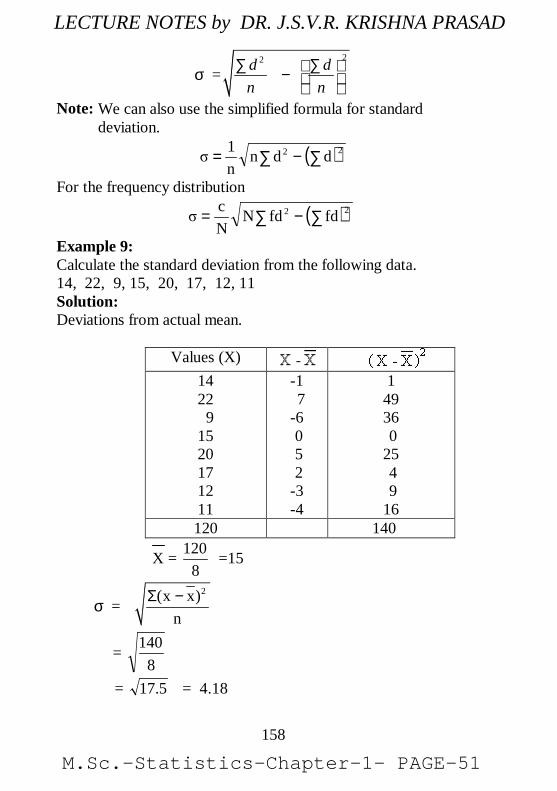
Note: We can also use the simplified formula for standard deviation.

( )22 ddnn1

∑∑ −=

For the frequency distribution

( )22 fdfdNNc

∑∑ −=

Example 9:Calculate the standard deviation from the following data.14, 22, 9, 15, 20, 17, 12, 11Solution:Deviations from actual mean.

Values (X)1422 91520171211

-1 7-6 0 5 2-3-4

14936 025 4 916

120 140

X =8

120 =15

σ =2(x x)

nΣ −

=8

140

= 5.17 = 4.18



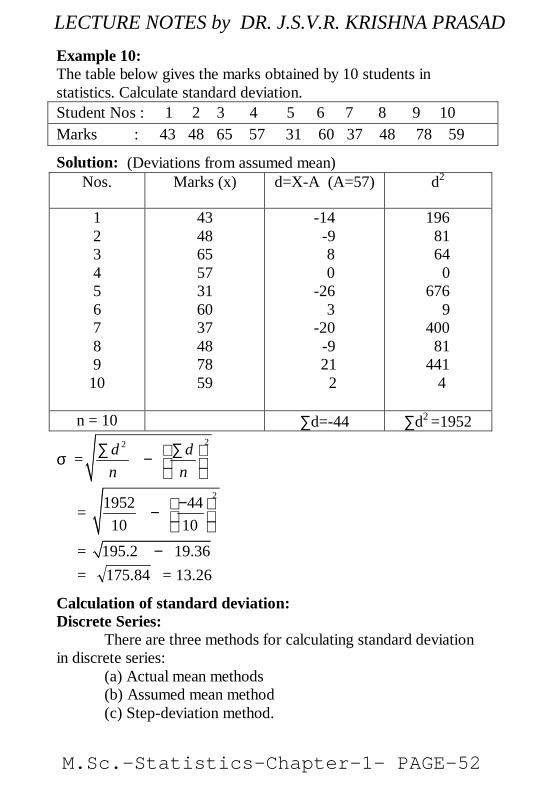
Example 10:The table below gives the marks obtained by 10 students instatistics. Calculate standard deviation.Student Nos : 1 2 3 4 5 6 7 8 9 10Marks : 43 48 65 57 31 60 37 48 78 59

Solution: (Deviations from assumed mean)Nos. Marks (x) d=X-A (A=57) d2

123456789

10

43486557316037487859

-14-9

8 0-26 3-20

-9 21 2

196 81 64 0676 9400 81441 4

n = 10 ∑d=-44 ∑d2 =1952

σ =22d d

n n∑ ∑ −

=21952 44

10 10− −

= 195.2 19.36− = 84.175 = 13.26

There are three methods for calculating standard deviationin discrete series:

(a) Actual mean methods(b) Assumed mean method(c) Step-deviation method.

Calculation of standard deviation:Discrete Series:



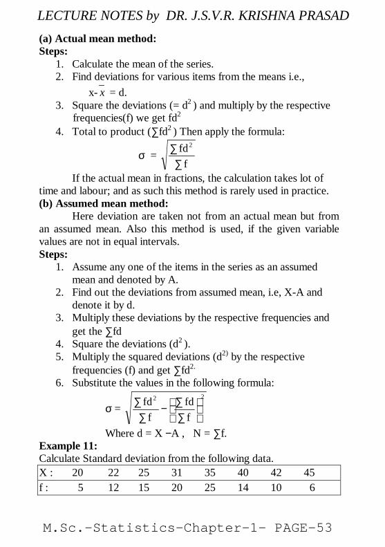
(a) Actual mean method:Steps:

1. Calculate the mean of the series.2. Find deviations for various items from the means i.e.,

x- x = d.3. Square the deviations (= d2 ) and multiply by the respective frequencies(f) we get fd2

4. Total to product (∑fd2 ) Then apply the formula:

σ =f

fd2

∑∑

If the actual mean in fractions, the calculation takes lot oftime and labour; and as such this method is rarely used in practice.(b) Assumed mean method:

Here deviation are taken not from an actual mean but froman assumed mean. Also this method is used, if the given variablevalues are not in equal intervals.Steps:

1. Assume any one of the items in the series as an assumedmean and denoted by A.

2. Find out the deviations from assumed mean, i.e, X-A anddenote it by d.

3. Multiply these deviations by the respective frequencies andget the ∑fd

4. Square the deviations (d2 ).5. Multiply the squared deviations (d2) by the respective

frequencies (f) and get ∑fd2.

6. Substitute the values in the following formula:

σ =22

ffd

ffd

∑∑

−∑

∑

Where d = X −A , N = ∑f.Example 11:Calculate Standard deviation from the following data.X : 20 22 25 31 35 40 42 45f : 5 12 15 20 25 14 10 6



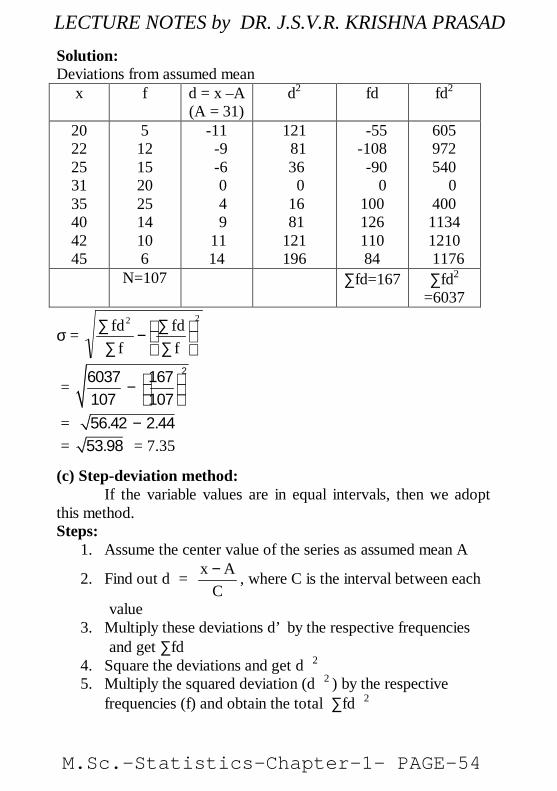
Solution:Deviations from assumed mean

x f d = x –A(A = 31)

d2 fd fd2

2022253135404245

51215202514106

-11-9-6

0 4 9 1114

121 81 36 0 16 81121196

-55-108

-90 010012611084

605972540 040011341210

1176N=107 ∑fd=167 ∑fd2

=6037

σ =22

ffd

ffd

∑∑

−∑

∑

= −

26037 167107 107

= 2.44. −56 42 = .53 98 = 7.35

(c) Step-deviation method:If the variable values are in equal intervals, then we adopt

this method.Steps:

1. Assume the center value of the series as assumed mean A

2. Find out d =C

Ax − , where C is the interval between each

value3. Multiply these deviations d’ by the respective frequencies

and get ∑fd4. Square the deviations and get d 2

5. Multiply the squared deviation (d 2 ) by the respectivefrequencies (f) and obtain the total ∑fd 2



6. Substitute the values in the following formula to get thestandard deviation.

Example 12:Compute Standard deviation from the following dataMarks : 10 20 30 40 50 60No.of students: 8 12 20 10 7 3Solution:

Marks x Fd =

1030x − fd fd 2

102030405060

8122010 73

-2-10123

-16-12 0 1014 9

3212 0102827

N=60 Σ fd =5 Σ fd 2

= 109

= 10605-

60109 2

×

= 100.0069-817.1 × = 100181.1 × = 1.345 × 10 = 13.45

deviation is almost the same as in a discrete series. But in acontinuous series, mid-values of the class intervals are to be foundout. The step- deviation method is widely used.

Calculation of Standard Deviation –Continuous series:In the continuous series the method of calculating standard



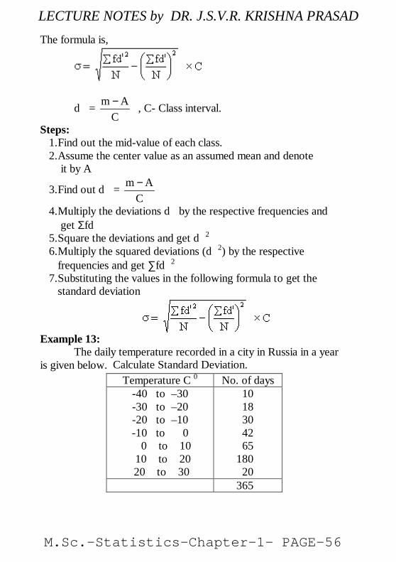
The formula is,

d =C

Am − , C- Class interval.

Steps:1.Find out the mid-value of each class.2.Assume the center value as an assumed mean and denote it by A

3.Find out d =C

Am −

4.Multiply the deviations d by the respective frequencies and get Σfd5.Square the deviations and get d 2

6.Multiply the squared deviations (d 2) by the respectivefrequencies and get ∑fd 2

7.Substituting the values in the following formula to get thestandard deviation

Example 13:The daily temperature recorded in a city in Russia in a year

is given below. Calculate Standard Deviation.Temperature C 0 No. of days

-40 to –30-30 to –20-20 to –10-10 to 0

0 to 10 10 to 20

20 to 30

1018304265

18020

365



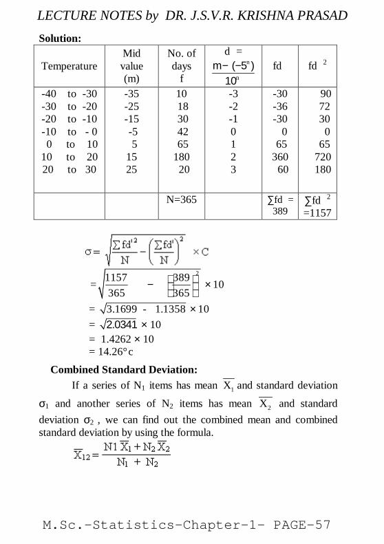
Solution:

TemperatureMidvalue(m)

No. ofdays

f

d =n

n

( )m− −510

fd fd 2

-40 to -30-30 to -20-20 to -10-10 to - 0 0 to 1010 to 2020 to 30

-35-25-15-5 51525

10 18 30 42 65180 20

-3-2-10123

-30-36-30 0 65360 60

90 72 30 0 65 720 180

N=365 ∑fd =389

∑fd 2

=1157

= − ×

389365

21157 10365

= ×3.1699 - 1.1358 10 = 2.0341 × 10 = 1.4262 × 10 = 14.26°c

σ1 and another series of N2 items has mean 2X and standarddeviation σ2 , we can find out the combined mean and combinedstandard deviation by using the formula.

Combined Standard Deviation:If a series of N1 items has mean X1 and standard deviation



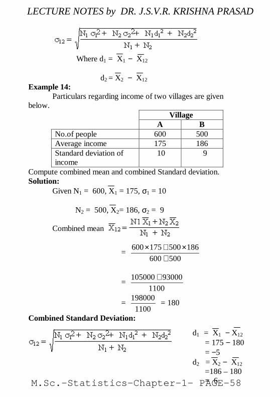
Where d1 = X1 − X12

d2 = X2 − X12Example 14:

Particulars regarding income of two villages are givenbelow.

VillageA B

No.of people 600 500Average income 175 186Standard deviation ofincome

10 9

Compute combined mean and combined Standard deviation.Solution:

Given N1 = 600, X1 = 175, σ1 = 10

N2 = 500, X2= 186, σ2 = 9

Combined mean

=500600

186500175600+

×+×

=1100

93000105000 +

=1100

198000 = 180

Combined Standard Deviation:

d1 = X1 − X12 = 175 − 180 = −5d2 = X2 − X12 =186 – 180 = 6M.Sc.-Statistics-Chapter-1- PAGE-58


σ12 =500600

365002560081500100600+

×+×+×+×

=1100

18000150004050060000 +++

=1100

133500

= 364.121 = 11.02.7.6.6 Merits and Demerits of Standard Deviation:Merits:

1. It is rigidly defined and its value is always definite andbased on all the observations and the actual signs ofdeviations are used.

2. As it is based on arithmetic mean, it has all the merits ofarithmetic mean.

3. It is the most important and widely used measure ofdispersion.

4. It is possible for further algebraic treatment.5. It is less affected by the fluctuations of sampling and hence

stable.6. It is the basis for measuring the coefficient of correlation

and sampling.

Demerits:1. It is not easy to understand and it is difficult to calculate.2. It gives more weight to extreme values because the values

are squared up.3. As it is an absolute measure of variability, it cannot be used

for the purpose of comparison.

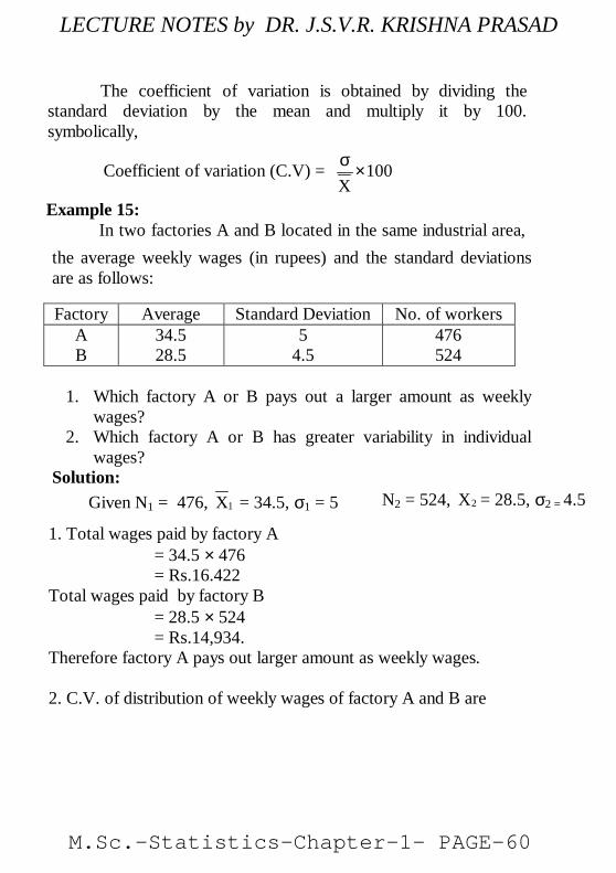
The coefficient of variation is obtained by dividing thestandard deviation by the mean and multiply it by 100.symbolically,

σ×Coefficient of variation (C.V) = 100

X



adiani

Typewritten text

Coefficient of Variation:

The coefficient of variation is obtained by dividing thestandard deviation by the mean and multiply it by 100.symbolically,

σ×

Example 15:In two factories A and B located in the same industrial area,

the average weekly wages (in rupees) and the standard deviationsare as follows:

1. Which factory A or B pays out a larger amount as weeklywages?

2. Which factory A or B has greater variability in individualwages?

Solution: Given N1 = 476, 1X = 34.5, σ1 = 5

Factory Average Standard Deviation No. of workersAB

34.528.5

54.5

476524

Coefficient of variation (C.V) = 100X

N2 = 524, X2 = 28.5, σ2 = 4.5

1. Total wages paid by factory A= 34.5 × 476= Rs.16.422

Total wages paid by factory B= 28.5 × 524= Rs.14,934.

Therefore factory A pays out larger amount as weekly wages.

2. C.V. of distribution of weekly wages of factory A and B are



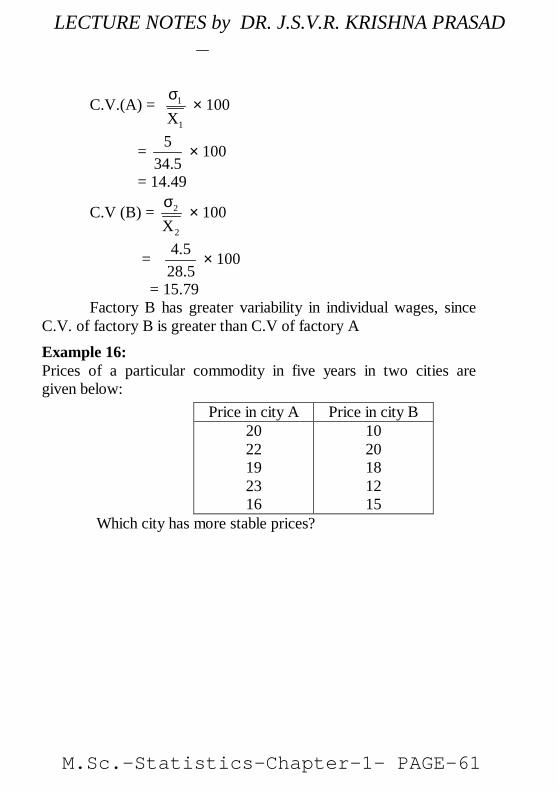
C.V.(A) = 1

1Xσ

× 100

=5.34

5× 100

= 14.49

C.V (B) = 2

2Xσ

× 100

=5.28

5.4× 100

= 15.79Factory B has greater variability in individual wages, since

C.V. of factory B is greater than C.V of factory AExample 16:Prices of a particular commodity in five years in two cities aregiven below:

Price in city A Price in city B2022192316

1020181215

Which city has more stable prices?



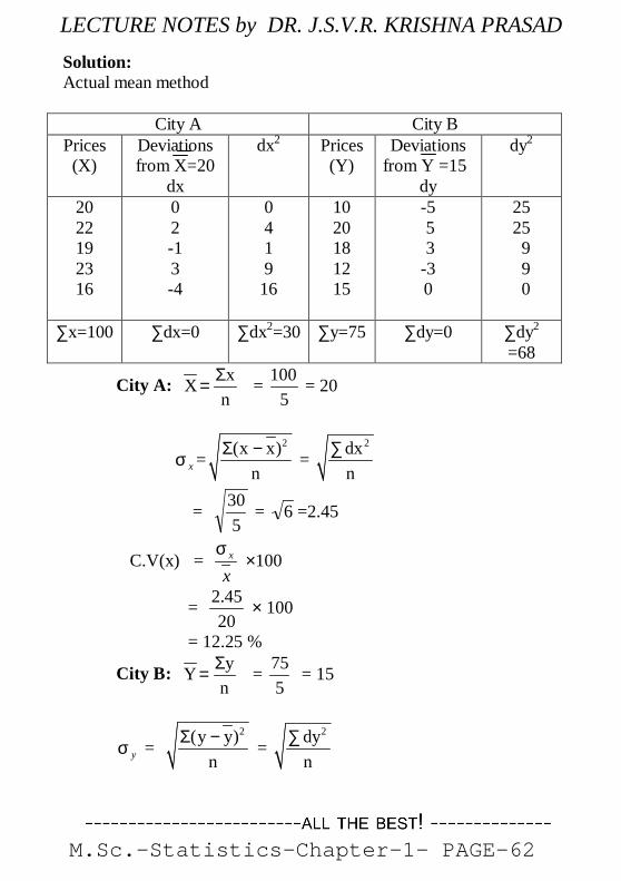
Solution:Actual mean method

City A City BPrices(X)

Deviationsfrom X=20

dx

dx2 Prices(Y)

Deviationsfrom Y =15

dy

dy2

2022192316

02-13-4

0419

16

1020181215

-5 5 3-30

2525 9 9 0

∑x=100 ∑dx=0 ∑dx2=30 ∑y=75 ∑dy=0 ∑dy2

=68

City A: xXn

Σ= =

5100 = 20

xσ =2(x x)

nΣ − =

2dxn

∑

=5

30 = 6 =2.45

C.V(x) = x

xσ

×100

=2045.2

× 100

= 12.25 %

City B: yYn

Σ= =

575 = 15

yσ =2(y y)

nΣ − =

2dyn

∑



adiani

Typewritten text

-------------------------ALL THE BEST! --------------

measures of central tendency - kcesmjcollege.in · mean = fd xa n ∑ =+ = 35 – = 35 – 4 = 31....

Documents