measurement traceability and uncertainty in … traceability and uncertainty in machine vision...
TRANSCRIPT

MIKES Metrology
Espoo 2007
Measurement Traceability and Uncertainty in
Machine Vision Applications
Björn Hemming
Dissertation for the degree of Doctor of Science in Technology to be presented with
due permission of the Department of Electrical and Communications Engineering, for
public examination and debate in Auditorium S1 at Helsinki University of
Technology (Espoo, Finland) on the 17th of December 2007, at 12 noon.

i
Abstract During the past decades increasing use of machine vision in dimensional
measurements has been seen. From a metrological view every serious measurement
should be traceable to SI units and have a stated measurement uncertainty. The first
step to ensure this is the calibration of the measurement instruments. Quality systems
in manufacturing industry require traceable calibrations and measurements. This has
lead to a good knowledge of measurement accuracy for traditional manual hand-held
measurement instruments. The entrance of rather complex computerised machine
vision instruments and optical coordinate measuring machines, at the production lines
and measurement rooms, is a threat or at least a challenge, to the understanding of the
accuracy of the measurement. Accuracies of algorithms for edge detection and camera
calibration are studied in the field of machine vision, but uncertainty evaluations of
complete systems are seldom seen. In real applications the final measurement
uncertainty is affected by many factors such as illumination, edge effects, the
operator, and non-idealities of the object to be measured.
In this thesis the use of the GUM (Guide to the Expression of Uncertainty in
Measurement) method is applied for the estimation of measurement uncertainty in two
machine vision applications. The work is mainly limited to two-dimensional
applications where a gray-scale camera is used. The described equipment for
calibration of micrometers using machine vision is unique. The full evaluation of
measurement uncertainty in aperture diameter measurements using an optical
coordinate measuring machine is presented for the first time.
In the presented applications the uncertainty budgets are very different. This confirms
the conclusion, that a detailed uncertainty budget is the only way to achieve an
understanding of the reliability of dimensional measurements in machine vision.
Uncertainty budgets for the type of the two described machine vision applications
have never previously been published.

ii
Tiivistelmä
Viime vuosikymmenien aikana konenäkö on yleistynyt yhä enemmän geometrisissä
mittauksissa. Metrologisesta näkökulmasta jokaisen mittauksen olisi oltava
jäljitettävissä SI-yksikköjärjestelmään ja jokaisella mittauksella tulisi olla tunnettu
mittausepävarmuus. Kaupallisesta näkökulmasta on tärkeää, että tavaran mitattavista
ominaisuuksista ei synny mittausvirheistä johtuvia kiistoja ostajan ja myyjän välillä.
Jos mittausepävarmuus on tunnettu, niin kalibroinnilla saadaan aikaan jäljitettävyys
perussuureeseen. Jäljitettävyys konenäkösovelluksissa pituuden SI-yksikköön metriin
saadaan aikaan pitkällä katkeamattomalla jäljitettävyysketjulla. Konepajoissa
laatujärjestelmät ovat jo pitkään edellyttäneet, että mittalaitteet ovat jäljitettävästi
kalibroitu. Jokaiseen kalibrointiin liittyy myös mittausepävarmuuslaskelma, jossa
tärkeimmät epävarmuuslähteet ovat mallinnettu. Optisten
koordinaattimittauskoneiden sekä muiden konenäköön perustuvien
mittausjärjestelmien mutkikkuus on suuri haaste mittausepävarmuuslaskelman
laatimiselle. Konenäkö sekä tarkkuuskysymykset konenäössä ovat paljon tutkittuja
aiheita, mutta kokonaisten mittausjärjestelmien epävarmuuslaskelmia laaditaan
edelleenkin erittäin harvoin. Epävarmuustekijöitä, jotka olisi otettava huomioon, ovat
valaistuksen, reunojen ja käyttäjän valintojen vaikutus yhdessä mitattavan kappaleen
mahdollisten puutteellisuuksien kanssa.
Tässä työssä tutkitaan GUM-menetelmän (Guide to the Expression of Uncertainty in
Measurement) käyttöä kolmessa konenäkösovelluksessa, joille esitetään
epävarmuuslaskelma. Neljäs esitettävä sovellus on apertuurien halkaisijan
mittaaminen optisella koordinaattimittauskoneella. Ensimmäistä kertaa tällaiselle
sovellukselle esitetään mittausepävarmuuslaskelma. Työn johtopäätöksenä on, että
yksityiskohtaisen epävarmuuslaskelman laatiminen on ainut keino saada käsitys
mittauksen virhelähteistä. Työ on rajattu kaksidimensionaalisiin mittauksiin, joissa
käytetään yhtä harmaasävykameraa.

iii
Preface
The research work behind this thesis is done at MIKES (Centre for Metrology and
Accreditation) as several research and development projects. A part of work described
in this thesis began when the author worked at VTT (Technical Research Centre of
Finland) during 1989 to 2000. The dimensional measurement group at VTT moved to
MIKES in 2000, due to a re-organization and strengthening of metrology in Finland.
The author is in gratitude to Prof. Timo Hirvi and Prof. Ulla Lähteenmäki for offering
research possibilities to the author. The author also wants to thank Dr Heikki Isotalo
for giving the initial inspiration to write this thesis. The author also greatly indebted to
his supervisor Prof. Erkki Ikonen for encouragement and inspiration. I thank the
Academy of Finland for financial support for this project.
The author wishes to thank Lic.Sc (Tech) Heikki Lehto for ideas and advice. The
author wishes also to thank Dr Antti Lassila for ideas and support. The author is
grateful to Mrs Jenni Kuva for proofreading this thesis. The author is grateful to M.Sc.
(Tech.) Ilkka Palosuo, Mr Asko Rantanen, M.Sc. Anu Fagerholm (former Tanninen)
and Mr Hannu Sainio at VTT for substantial co-work in projects related to this
dissertation. In the last phase of this work the author received spiritual support and
many helpful hints from M.Sc. Virpi Korpelainen, Dr Kaj Nyholm and Dr Mikko
Merimaa. The author thanks Mrs. Kirsi Tuomisto and M.Sc. (Tech.) Milla Kaukonen
for help with the final editing of the thesis. The author also thanks Prof. Henrik
Haggrén at the laboratory of Photogrammetry at TKK (Helsinki University of
Technology) for views and ideas
Furthermore I want to thank all my colleagues at MIKES and especially my
colleagues Ilkka, Raimo, Jarkko and Veli-Pekka, in the length group for help, patience
and support during the years at the new MIKES.
Last but not least I thank my wife Marja-Riitta and daughters Ella and Malin.
Björn Hemming

iv
List of Publications
This thesis consists of an overview and the following selection of the author’s
publications.
Publ. I
B. Hemming, I. Palosuo, and A. Lassila, “Design of Calibration Machine for Optical
Two-Dimensional Length Standards”, in Proc. SPIE, Optomechatronical Systems III,
Vol. 4902, pp. 670-678 (2002).
Publ. II
B. Hemming, E. Ikonen, and M. Noorma, “Measurement of Aperture Diameters using
an Optical Coordinate Measuring Machine”, International Journal of
Optomechatronics, 1, 297–311 (2007).
Publ. III
B. Hemming and H. Lehto, “Calibration of Dial Indicators using Machine Vision,”
Meas. Sci. Technol. 13, 45-49 (2002).
Publ. IV
B. Hemming, A. Fagerholm, and A. Lassila, “High-accuracy Automatic Machine
Vision Based Calibration of Micrometers”, Meas. Sci. Technol. 18, 1655-1660 (2007).

v
Authors Contribution
The development of the equipment described in Publ. I was a team project, where the
responsibility of the author was the machine vision hardware and software
development. The software was written with the assistance of M.Sc. (Tech.) Ilkka
Palosuo. The role of M.Sc. (Tech.) Ilkka Palosuo was the design of the mechanics of
the instrument. For Publ. I the author prepared the manuscript and the uncertainty
budget.
For Publ. II the author performed all measurements and analyses alone with the
exception of the verification with probing CMM (Coordinate Measuring Machine),
which was carried out together with M.Sc. (Tech.) Ilkka Palosuo. For Publ. II the
author prepared the manuscript.
For Publ. III the author designed and built the instrument and wrote the software. The
author also carried out all of the measurements and the uncertainty analysis. For Publ.
III the author prepared the manuscript.
For Publ. IV the author designed and built the instrument. The software was written
with the assistance of M.Sc. Anu Fagerholm. The author made all of the
measurements and all of the research work including the uncertainty analysis. For
Publ. IV the author prepared the manuscript.
The spread of the years of publication was partly due to the moving process to the
new MIKES building in 2005.

vi
List of abbreviations
1D One dimensional
2D Two dimensional
3D Three dimensional
BIPM International Bureau of Weights and Measures/
Bureau International des Poids et Mesures
CCD Charged coupled device
CCIR Comité International des Radiocommunications
CMC Calibration and Measurement Capability
CMM Coordinate Measuring Machine
EAL European Cooperation for Accreditation of Laboratories
GUM Guide to the Expression of Uncertainty in Measurement
LED Light-emitting diode
METAS Bundesamt für Metrologie
MIKES Centre for Metrology and Accreditation/ Mittatekniikan keskus
NIST National Institute of Standards and Technology
NMI National Measurement Institute
NPL National Physical Laboratory
PTB Physikalisch Technische Bundesanstalt
SPIE The International Society for Optical Engineering
TKK Helsinki University of Technology (formerly abbreviated HUT)
VDI/VDE Verein Deutscher Ingenieure/Verband der Elektrotechnik,
VTT Technical Research Centre of Finland

vii
List of symbols
dx Distortion in x-axis
dy Distortion in y-axis
k Coverage factor
k1 Coefficient for 2nd order radial distortion
k2 Coefficient for 4th order radial distortion
ρ Distance from image centre
Sx Scale factor for x-axis
Sy Scale factor for y-axis
u(x) Standard uncertainty for the input estimate
uc(y) Combined standard uncertainty
x Input estimate
X Input quantity
Xp Undistorted x-coordinate of a point in the image
y Estimate of measurand
Y Measurand
Yp Undistorted y-coordinate of a point in the image

Table of contents Abstract iTiivistelmä iiPreface iiiList of publications ivAuthors contribution vList of abbreviations viList of symbols vii
1. Introduction........................................................................................................... 1
2. Measurement Traceability and Uncertainty.......................................................... 4
2.1. Measurement Traceability ............................................................................ 4
2.2. Measurement Uncertainty............................................................................. 7
2.3. Research Question ........................................................................................ 9
2.4. Progress in this work................................................................................... 10
3. Calibration of Reference Standards for Machine vision..................................... 13
3.1. Calibration of 2D standards ........................................................................ 13
3.2. Development of equipment for calibration of 2D standards....................... 15
3.3. Discussion ................................................................................................... 18
4. The Use of Optical Coordinate Measuring Machines......................................... 20
4.1. Introduction to CMM.................................................................................. 20
4.2. Task specified uncertainty for CMM.......................................................... 22
Sensitivity analysis.............................................................................................. 23
Experimental method using calibrated objects ................................................... 23
Computer simulation and virtual CMM.............................................................. 24
4.3. Measurement of apertures using an optical CMM...................................... 25
Verification measurements ................................................................................. 28
4.4. Discussion ................................................................................................... 29
5. Machine Vision Based Calibration Equipment................................................... 30
5.1. Introduction to Machine Vision .................................................................. 30
5.2. Camera Calibration in Machine Vision ...................................................... 33
An example of camera calibration ...................................................................... 34
5.3. Calibration of Dial Indicators with Machine Vision................................... 35
5.4. Calibration of Micrometers with Machine Vision ...................................... 37
5.5. Discussion ................................................................................................... 41
6. Conclusions......................................................................................................... 44
References................................................................................................................... 47

- 1 -
1. Introduction
In the manufacturing industry the tradition of systematic measurements is long. At the
time of the first industrial revolution, James Watt invented the screw micrometer in
1772 [1]. One important step was the invention of gauge blocks in 1896 by C. E.
Johansson in Sweden [2]. For the manufacturing industry the gauge blocks have been
the basic reference in the calibration of simple handheld instruments such as callipers
and micrometers. The first coordinate measuring machine (CMM) with three axes was
manufactured by the Swiss company SIP already in 1930. An important invention for
machine vision was the CCD camera, developed in the 1960s.
Systematic measurement with known uncertainty is one of the foundations of science
and technology. Measurements are central in industrial quality control and in most
modern industries the costs bound up in taking measurements constitute 10-15 % of
production costs [3]. Quality management is important in any industry where the
product is assembled from hundreds of parts, which have to fit together. Therefore,
the measuring instruments are calibrated and the users must have knowledge of the
measuring uncertainties when they verify that the products are within specified
tolerances. If the product is not within specified tolerances, it is useless to send it to
the customer. If the product seems to be within specifications, but rejected by the
customer, the economic loss is even bigger. Therefore, there is a clear connection
between understanding of measurement errors and economics.
In addition to the aforementioned requirements, another challenge is the demand for
more accurate measurements. In figure 1 this demand, as seen by the National
Physical laboratory (NPL) is illustrated. This increasing demand of accuracy is not
narrowed to special cases or small volume production. An example from mass
production where high accuracy is needed is the manufacturing of hard disk
components and fuel injection systems [4].

- 2 -
During the last 20 years many advances in measurement instruments have also caused
new challenges for uncertainty evaluation. First digital data processing made it
possible to develop programmable CMM’s. Then machine vision [5, 6] was
developed and used for inspection and measuring tasks in industry.
Figure 1. The demand for lower measurement uncertainty in dimensional
measurements [7]
Finally, during the last ten years machine vision capabilities were installed to some
CMM’s and the Video Measuring Machine or optical CMM was developed. However,
some new problems have emerged. According to Ref. [8] the uncertainty for CMM
measurements is in many cases simply a guess from an experienced operator.
Moreover, there are situations where intuition and experience may fail dramatically
[9]. In machine vision, which is a younger technology than CMM, the situation is
roughly the same or even worse. Machine vision has, during the recent years, gained
from the cheaper computing costs. This means that more and more machine vision
applications are developed all the time.
The amount of work and complexity in a measurement uncertainty calculation
corresponds to the complexity of the measurement. If a part was previously measured

- 3 -
using a mechanical vernier or micrometer calliper and is now measured by machine
vision, a lot of work would be needed to find the error sources of the new system. It
seems that the measurement uncertainty and traceability chain is no longer as well
known as it was before. In this thesis it is shown how traceability and measurement
uncertainty are achievable in machine vision applications using the GUM method
[10].

- 4 -
2. Measurement Traceability and Uncertainty
In 1799 in Paris, the Metric System was established by the deposition of two platinum
standards representing the metre and the kilogram. This was the first beginning of the
present International System of Units, the SI system [11]. From year 1983 the
definition of the metre is given as the length of the path traveled by light in vacuum
during a time interval of 1/299 792 458 of a second. Some concepts in the practical
realisation work of the SI-unit metre are described in the following.
2.1. Measurement Traceability
A traceability chain is an unbroken chain of comparisons, all having stated
uncertainties. This ensures that a measurement result or the value of a standard is
related to references at the higher levels, ending at the realisation of the definition of
the unit.
The definition of calibration according to Ref. [12] is the following: “Set of
operations that establish, under specified conditions, the relationship between values
of quantities indicated by a measuring instrument or measuring system, or values
represented by a material measure or a reference material and the corresponding
values realised by standards.” The most important measuring instruments in length
and dimensional metrology are the laser interferometers, line scales, gauge blocks,
ring gauges and form standards. Important reference standards used in coordinate
metrology are step gauges and ball plates. All instruments and reference standards
have to be calibrated regularly [13]. The result of the calibration is a certificate
usually containing a table where instrument readings can be compared to reference
values. It is then up to the end user how he will use the certificate and its results.

- 5 -
Sometimes the procedure, when a scale factor between a transducer output and a
physical unit is established, is also called calibration. In machine vision literature
there are many articles about camera calibration. Usually the purpose is to define the
relation between the captured image and world coordinates.
Every measurement intended to be reliable should have a traceability chain to the
corresponding definition of the SI-unit (figure 2). At MIKES there are six iodine-
stabilized lasers. Thanks to advances in laser technology the traceability for these
secondary frequency standards was recently achieved from a femtosecond frequency
comb [14, 15]. The traceability to the frequency comb comes from a primary
frequency standard, a Cs atomic clock. The wavelengths of the lasers of the primary
interferometers are calibrated against the wavelengths of the iodine-stabilized lasers.
These primary interferometers are then used to calibrate other reference instruments,
such as gauge blocks, step gauges, line-scales and other laser interferometers [16].
Interferometrically calibrated gauge blocks are used to calibrate other gauge blocks
using a gauge block comparator [17].

- 6 -
Figure 2. Traceability chain from national standard to product.
For example, a micrometer calliper may be used at factory floor to measure a product.
The calibration of a micrometer calliper using calibrated gauge blocks [18] is simple
and straightforward and the user has an understanding of both the calibration and the
measuring process. It is also an advantage that the calibration using gauge blocks is
quite similar to the measurement of the products. If the manual measurement of
products is replaced by a machine vision based inspection system the benefits, such as
speed, are obvious but the measuring process, and error sources too, get more
complex.
In trade comparability and reliability of measurements are important, between buyer
and seller. This gives a requirement of reliability and traceability, which cannot be
neglected, when mechanical measurement is replaced by machine vision in industry.
± 0.1 mm
± 0.0001 mm
± 0.005 mm
Example of traceability chain Definition of the unit
Frequency comb
Iodine stabilized laser
Laser interferometer
Gauge block, line scale
Gauge blocks, standards
NMI:
-Realization
-Primary standards
Accredited laboratory:
-Reference standards
Calibration laboratory at factory
-Working standards
Measurement equipment at
production and quality control
Measurement of product

- 7 -
2.2. Measurement Uncertainty
In a measuring process, there are several factors that influence the measuring results
and measuring uncertainty. The most important factors are properties of the used
measuring instrument and calibration and how well they are suited for measuring the
object (figure 3).
Figure 3. Factors affecting a measuring process (after [19]).

- 8 -
In the documentation of GUM [10] general rules for evaluating and expressing
measurement uncertainty are described. In the GUM the estimate of the measurand Y,
denoted by y, is obtained from input quantities x1, x2, ... , xn representing N quantities
X1, X2, ... , XN. The output estimate y, which is the result of the measurement, is given
by:
(1)
The standard uncertainties for the input estimates are noted as u(xi). If the input
quantities are independent, the combined standard uncertainty uc(y) is obtained from:
. (2)
Usually the combined standard uncertainty is multiplied by the coverage factor k=2,
to express the expanded uncertainty at a 95% confidence level.
Equation 1 represents the measurement model. In a simple measurement using a
handheld instrument like a vernier calliper, the measurement model is trivial with only
three or four input estimates. However, in a machine vision system containing
hundreds of program lines in its software, the measurement model is quite complex.
An example of this is seen in Publ. IV.
A lot of work has been done on accuracy problems in photogrammetry and accuracy
questions in camera calibration in machine vision. However, measurement uncertainty
for a whole system and the concepts of GUM are rare in these fields. There are some
exceptions, which should be mentioned. In metrology institutes, machine vision has
for some time been used for interferometric gauge block calibration [20], flatness
measurements with Fizeau interferometers [21], line scale measurements [22] and
photomask measurements [23]. For these applications a detailed analysis of
measurement uncertainty is normally found.
)()( 22
1
2i
N
i ic xu
xfyu ∑
=⎟⎟⎠
⎞⎜⎜⎝
⎛=
δδ
)( 21 n,...,x,xxfy =

- 9 -
2.3. Research Question
The area of interest in this thesis is measurement traceability and uncertainty in
dimensional machine vision applications. This thesis is limited to two-dimensional
applications where one gray-scale camera is used. It might be argued that the
principles of GUM are well known and that also accuracy has been studied in the vast
literature of machine vision. However, the principles of GUM have been applied only
in very few machine vision applications, and there are gaps which should be filled. In
this thesis the research question is:
what is the role and benefit of an uncertainty evaluation during the
development of a measurement application where machine vision is used for a
dimensional measurement?
On one hand, the development of a measurement application might be design,
building and testing of new measurement equipment. On the other hand, in industry,
where machine vision is used for quality control, there is a need for reliable
measurements. Therefore the research question is divided into two subquestions:
how can uncertainty sources be evaluated during design of a measurement
instrument based on machine vision ?
how is it possible to achieve traceability and reliability in a measurement
based on machine vision ?
In this thesis applications using four different measurement systems are described;
optical CMM, measurement of two-dimensional (2D) standards and two calibrations
systems for micrometers and dial indicators. The original motivation for these
applications was not only to answer the abovementioned research questions. Still the
second subquestion is addressed in Publ. II and section 4 where the use of a
commercial optical CMM is analysed. The other publications describe uncertainty
budgeting during design of instruments.

- 10 -
The applications look quite different but on the other hand the 2D standard measuring
instrument is in principle an optical CMM. Also, it should be noted that the border
between optical CMM and machine vision will fade away in the future [24]. The
requirement of traceability for production measurements where machine vision is
used, causes a need of calibration standards such as line scales or 2D standards. These
standards are in turn also calibrated using machine vision. Examples of traceability
chains are also presented and discussed in this thesis. The hypothesis of this thesis is
that a thorough uncertainty evaluation is crucial during the development of a
measurement application where machine vision is used.
2.4. Progress in this work
Publ. I.
In dimensional metrology the traceability comes from lasers with stable and well-
known wavelengths. An example is the calibration of line-scales using laser-
interferometers. Using line-scales, measurement machines can be calibrated one axis
at a time. One quick method to check and calibrate optical coordinate measuring
machines is to use 2D standards.
A design and development project aiming at a new calibration service for two-
dimensional length standards was started in 2000 at MIKES. In the developed
measurement equipment the expanded (k=2) measurement uncertainty is Q[0.094;
0.142 L]1 µm, where L is the position in metres. This result is obtained by applying
error compensation methods to the pitch error of the movements and to flatness errors
of the mirror block. The achievable measurement uncertainty of 0.1 µm (k=2) for a
position at 150 mm is sufficient for most calibrations.
1 Expression for combination of non-length dependent and length (L) dependent uncertainty
components: Q[A; B L] = (A2 + (B L)2 )1/2

- 11 -
Publ. II
Apertures are used in photometry and radiometry to limit a precisely known area of
the incoming radiation field in front of a detector. The known area is needed to
determine such quantities as illuminance or irradiance.
An optical CMM or video measurement machine is used for the measurement of mean
diameters of apertures. It is obvious that the measurement uncertainty, even of a high
accuracy optical CMM, cannot be as good as that of a dedicated aperture
measurement facility in a National Measurement Institute. However, if the required
standard uncertainty for the mean diameter is not less than 1 µm, the optical CMM is
both useful and easy to use for aperture area measurements. In a comparison with
probing CMM excellent agreement was found. This report presents the first full
uncertainty analysis of the aperture area measurement by optical CMM, including
confirmation of the results by Monte-Carlo method.
Publ. III
With machine vision it is possible to check hundreds of points on the scale of a dial
indicator, giving new insight into error sources of the dial indicator. The article
describes a machine vision based system for the calibration of dial indicators
developed at MIKES. With the developed machine vision system the uncertainty of
the reading and interpretation of the pointer is of the same order as when a dial
indicator is calibrated manually. In the article the calculation of the measurement
uncertainty is described in detail. Uncertainty evaluation according to GUM has not
previously been published for an automatic measurement system for dial indicators.

- 12 -
Publ. IV
The manual calibration of a micrometer calliper according to IS0 3611 is done by
using ten gauge blocks. This gives only a rough figure for the accuracy of the
instrument and is not a complete check of the scale. Using automatic machine vision
based systems; the calibration of measurement instruments can be extended.
Equipment for the automatic calibration of micrometers is presented. The purpose of
the study is to show the feasibility of traceable calibration of micrometers using
machine vision. Another similar system is not known to the author and therefore it is
probably the first of its kind. Detailed uncertainty analysis following the
recommendations of GUM is given.

- 13 -
3. Calibration of Reference Standards for Machine vision
3.1. Calibration of 2D standards
One important reference standard in high accuracy machine vision applications is a
line-scale. In Finland line scales of length less than 1160 mm can be calibrated using a
line-scale interferometer at MIKES [22, 25]. The uncertainty of the calibration of line-
scales is Q[62; 82L] nm (k=2), where L is the length of the scale in metres. Longer
line-scales and measurement tapes up to 30 m can be calibrated interferometrically at
the 30 m measurement rail in MIKES.
Although traceability for a machine vision measurement can be achieved by a line-
scale, a two dimensional standard or calibration grid is a very useful tool in camera
calibration. The advantage is that a large measurement area and orthogonality error is
covered in a single measurement. A practical disadvantage is that the correction of the
misalignment of the two-dimensional standard depends on the selected alignment
criteria or selected reference points. This makes it difficult to compare different
calibration certificates for a two-dimensional standard. For a line scale it is much
easier to compare the results and to document the stability.
Several instruments for measurements of 2D standards and photomasks with high
accuracy have been developed during the recent ten years [26, 27, 28, 29, 30]. Error
separation is also used in many applications [31, 32, 33]. In the manufacturing of
integrated circuits, lithographic processes are used where accurate 2D positioning is
needed. Therefore, the needs of these applications has led to a field called mask
metrology. State of the art systems used in this industry achieve positional
repeatabilities of the order of 10 nm [34].

- 14 -
The most accurate measurements systems for 2D measurements are equipped with
interferometers and orthogonal two-plane mirror reflectors. The optical detection of
the features and structures on the mask or 2D standard is done using a microscope,
usually equipped with a camera. Such instruments are nowadays found in large
national measurement institutes such as NPL in Britain, Physikalisch Technische
Bundesanstalt (PTB) in Germany, Bundesamt für Metrologie (METAS) in
Switzerland and National Institute of Standards and Technology (NIST) in the United
States. Usually the 2D standard is measured in four different positions, each turned by
90°. The measurement uncertainty for the instrument at NPL is
0.06 µm (k=2) [26]. In another paper the instrument is verified to achieve the
uncertainty of 0.08 µm (k=2), for an 80 mm x 80 mm grid [34].
The measurement range of the instrument developed in METAS is 300 mm x 400
mm. The equipment in METAS is especially developed for photomask measurements,
but it can also be used for various calibration tasks for line scales and 2D standards.
An important property of the instrument in METAS is that the Abbe error of the
measurement beams is neglible [27]. In calibration measurements for the equipment
using a 400 mm quartz line scale mirror, corrections of 40 nm and 140 nm were
derived [27]. The final measurement uncertainty is not reported in Ref. [27] but
according to the CMC database of BIPM it is about 0.04 µm (k=2) for a 100 mm x
100 mm grid. In a comparison between NPL and PTB for a 120 mm x 120 mm 2D
standard the agreement between the results was within ±0.1 µm [23]. The dominating
uncertainty source of the instrument in NPL is Abbe error [23]. Other uncertainty
sources; discussed in the literature, are the flatness and orthogonality deviations of the
two-plane mirrors and temperature effects, such as thermal expansion and refractive
index of air.

- 15 -
3.2. Development of equipment for calibration of 2D standards
A design and development project aiming at a new calibration service for two-
dimensional length standards was started in 2000 at MIKES. The technical
requirement for the new calibration machine was an expanded uncertainty in
calibrations of 0.1 µm (k=2) over the measuring range of 150 mm x 150 mm.
The operating principle of the device is based on use of a moveable xy-stage on air
bearings. The mechanics of the equipment consist of two linear granite rails, two
linear stepping motor actuators, and ten air bearings (figure 4). The two-dimensional
standard under calibration is fastened to the Zerodur mirror block using three suction
pads. A three-axis plane-mirror heterodyne interferometer system measures the
position of the mirror block. The optical components of an old lithography machine
were used. Unfortunately the use of this old hardware lead to an Abbe offset of 15
mm between the laser beams and the two-dimensional standard under calibration.
Using online compensation, based on measured data on pitch angle, the Abbe error
can be reduced but not completely eliminated.
The position of the feature in the standard is detected with a ½” CCD camera,
equipped with a telecentric lens. The scale factor is from 0.3 µm/pixel to 6 µm/pixel,
depending on the selected lens. The achieved expanded (k=2) uncertainty for a
position measurement is Q[0.094; 0.142 L] µm, where L is the position in metres. For
a length of 100 mm this equals 0.095 µm.

- 16 -
Figure 4. Calibration instrument for two-dimensional standards.
The graduation marks of the standard are positioned in turn at the centre of the image.
The position of the graduation mark is measured using template matching or gray-
scale correlation [35]. An alternative method to measure the position of the feature
would be to use subpixel detector and minimization [36], or fitting of lines on the grid
mark edges [37]. In some cases the Hough transform is a robust method to find lines
in an image [38, 39, 40]. In this application gray-scale correlation was selected
because it gives a good combination of accuracy and speed [41].
In order to test performance of the device, a 50 mm glass line scale was measured
using the equipment. A line was used as a template and results were averaged from
five measurements (figure 5). The differences of the results compared to
measurements of MIKES’ line scale interferometer were typically below 60 nm. The
expanded uncertainty of the reference results for the particular scale were 90 nm
(k=2). The line scale was too short to reveal errors due to temperature and mechanics,
but the good result is a verification of the chosen image processing and machine
vision parts of the developed system.
Zerodur plate
Interferometer
optics
Stepping motor
actuator
Camera
Laser
Mirror block
Standard to be
calibrated
Objective
Stone table

- 17 -
-0.15
-0.10
-0.05
0.00
0.05
0.10
0.15
0 5 10 15 20 25 30 35 40 45 50
Position / mm
Dev
iatio
n / µ
m
Figure 5. Deviation between results from the developed instrument and MIKES line-
scale interferometer for a 50 mm line-scale [41].
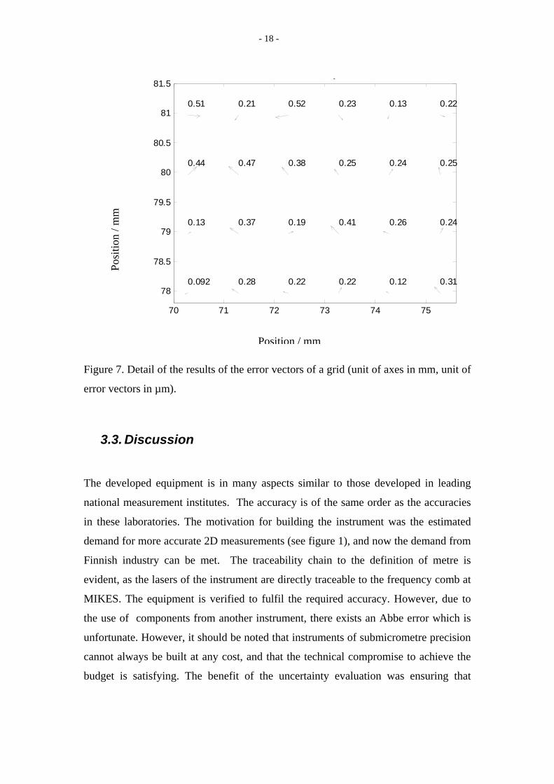
Shown in figure 6 is an example of a standard of the size 100 mm x 100 mm
calibrated with the instrument. In figure 7, the result of the calibration is shown. The
user of a small optical CMM may use this kind of standard to measure the scale and
orthogonality errors of the CMM. In Publ. I the uncertainty budget is presented, and
it was found that the largest uncertainty source in the equipment is the uncompensated
part of the previously mentioned Abbe error.
Figure 6. A photograph of the standard (left) and a drawing of the same standard
(right). The larger grid has 10 mm intervals and in the middle there is a denser grid
with 1 mm intervals.
- 18 -
70 71 72 73 74 75
78
78.5
79
79.5
80
80.5
81
81.5y
0.22
0.25
0.24
0.31
0.13
0.24
0.26
0.12
0.23
0.25
0.41
0.22
0.52
0.38
0.19
0.22
0.21
0.47
0.37
0.28
0.51
0.44
0.13
0.092
Figure 7. Detail of the results of the error vectors of a grid (unit of axes in mm, unit of
error vectors in µm).
3.3. Discussion
The developed equipment is in many aspects similar to those developed in leading
national measurement institutes. The accuracy is of the same order as the accuracies
in these laboratories. The motivation for building the instrument was the estimated
demand for more accurate 2D measurements (see figure 1), and now the demand from
Finnish industry can be met. The traceability chain to the definition of metre is
evident, as the lasers of the instrument are directly traceable to the frequency comb at
MIKES. The equipment is verified to fulfil the required accuracy. However, due to
the use of components from another instrument, there exists an Abbe error which is
unfortunate. However, it should be noted that instruments of submicrometre precision
cannot always be built at any cost, and that the technical compromise to achieve the
budget is satisfying. The benefit of the uncertainty evaluation was ensuring that
Posi
tion
/ mm
Position / mm

- 19 -
traceable measurements of the required accuracy can be made. This conclusion is a
partial, although not a complete answer to the research question.
As for any new measurement instrument in a NMI (National Measurement Institute),
the participation in an interlaboratory comparison would be desirable, to finally prove
the measurement capability and to give ideas for improvements to the instrument.

- 20 -
4. The Use of Optical Coordinate Measuring Machines
4.1. Introduction to CMM
The coordinate measuring machine is a universal measurement machine in
dimensional metrology [42]. With these machines complex structures, for example,
parts of engines and pumps, can be measured. The size or measurement volume of a
CMM does vary a lot. A big CMM in the car industry may have axes of a length of
several metres and a CMM for the measurement of microsystem components has an
axis length of some centimetres [43, 44]. A complete description of the CMM and the
measurement uncertainty of CMM is beyond the scope of this dissertation [45, 46,
47,48]. In some studies laser interferometers are used to get traceability and achieve a
small measurement uncertainty [49]. Also error compensation methods are applied
[50]. In one specific work error compensation is applied for a cylinder [51].
Measurement comparisons between laboratories using error separation methods have
also been done [ 52].
The measurement uncertainty depends not only on the errors of the CMM but also on
fitting algorithms of the measured feature and sampling. There are only few
guidelines for the calibration of a CMM. One example can be found in Ref. [53].
One type of CMM is an optical CMM, which is a CMM equipped with a camera
instead of a contacting probe. Typical lens magnifications provide a resolution of 0.5
µm/pixel to 2 µm/pixel [4]. The optical CMM is ideal for non contact 3D
measurements of small elastic parts and features. Typical claimed measurement
uncertainties for commercial optical CMM’s range from 0.8 µm to 6 µm [54, 55].
A third type of CMM is equipped with an opto tactile sensor. Here an optical fibre is
used for probing and the position of the fibre is measured by a camera [56].

- 21 -
The measurement uncertainty of a specific CMM measurement task is a widely
studied subject and in figure 8 one approach is shown. A similarity between optical
CMM’s and machine vision is the importance of the illumination. Different operators
may perform different illumination selections and the results of the dimensional
measurements may therefore be different. Also the selected measurement strategy
may affect the results [57]. Therefore it can be said that the skill of the user is critical
for successful CMM measurements and figure 8 is a somewhat idealized presentation
because it hides the human factor.
Figure 8. Factors affecting a CMM measurement [9].
In table 1, the relative distribution of uncertainty components for measurements using
a CMM and an optical CMM are presented. The effect of the operator is very high for
instruments operated in the industry. Especially for the case of the optical CMM the
operator is responsible for the selection of illumination, measurement strategy and
alignment compensation.
Table 1. Fractional distribution of uncertainty components for measurements using a
CMM and an optical CMM [58].
Operator Instrument Environment Object
Probing CMM 30-50 % 5-20 % 5-20 % 10-30 %
Optical CMM 50-70 % 5-20 % 2-5 % 20-40 %
In metrology it is customary to test the claimed measurement capabilities by arranging
comparisons where the same artifact is circulated and measured by different
participants. As pointed out by a national comparison in Finnish industry [59], many

- 22 -
users do not know the real measurement uncertainties. In an other comparison for 11
optical and 12 mechanical CMM’s, the results showed agreement with the reference
values within the reference uncertainty, and also showed that optical CMM
measurements can be as good as mechanical CMM measurements [60 ].
4.2. Task specified uncertainty for CMM
Although the question of measurement uncertainty for a specific measurement made
with a CMM, has been intensively studied, there is still no single clear solution to this
problem. In a survey [61] published in 2001 the following possibilities are classified
as:
- Sensitivity analysis
- Expert judgement
- Experimental method using calibrated objects (Substitution method)
- Computer simulation (Virtual CMM)
- Simulation by constraints
- The expert CMM
- Statistical estimations from measurement history
- Hybrid methods
In [24] the possibilities are classified and presented as:
- Expert judgement
- Uncertainty evaluation based on step gauge results
- Simplified substitution without corrections
- Substitution according to ISO15330-3
- Uncertainty evaluation based on geometric errors together with simulation
(PTB software Kalkom Megakal and VCMMtool)
- Virtual CMM (OVCMM)

- 23 -
In the following, three of the above approaches are discussed: sensitivity analysis,
substitution method and virtual CMM. One conclusion of the survey was that there
are large classes of coordinate measuring systems that have only been partially
addressed in the literature such as photogrammetry systems and vision based CMM’s
[61]. Another conclusion was that none of the methods for task specific uncertainty
appear to successfully address the interaction between sampling strategy and possible
part form error. During the preparation of this thesis the new ISO 15530 series of
standards “GPS- Coordinate measuring machines – Techniques for determining the
uncertainty of measurements” was not yet completely published with the exception of
ISO 15530:3 describing the substitution method. In the future, the remaining parts
describing expert judgement, virtual CMM and methods using statistics from
measurement history and methods using uncalibrated workpieces are expected to be
published.
Sensitivity analysis
For simple measurements where a well defined mathematical model of the
measurements can be formulated, the GUM method is easy to use and this is called
sensitivity analysis in [61]. For example, when a CMM is used for a simple length
measurement, the measurement model is also relatively simple and the sensitivity
coefficients can be determined. For a 2D measurement task the measurement model is
already of considerable complexity.
Experimental method using calibrated objects
This method, also called the substitution method, is based on the comparator
principle. If a reference work piece, almost identical to the object to be measured is
available, repeated measurements on both are performed. This means that it would be
good to have quite a large number of different calibrated references avalable. One
advantage with this straightforward method is that it is simple and can be brought and
communicated to the user. On the other hand, any differences (for example thermal
expansion coefficient) between the reference part and the object to be measured can
lead to unwanted uncertainties [61].

- 24 -
Although the substitution method is valuable, it is not the complete solution to the
task specific uncertainty problem [61]. Because the full substitution method is
regarded as tedious a simplified substitution method is suggested in [24].
Computer simulation and virtual CMM
A straightforward application of GUM becomes very difficult or perhaps impossible
in complex measurement processes such as form measurement and 2D or 3D
coordinate measurements. In these measurements, digital filtering of measurement
points is used, and at the points geometric elements are fitted. The question is how to
formulate a measurement model with sensitivity coefficients. If for example a hole is
measured by fitting a circle on say 100 measured (x, y) points, what is the contribution
to diameter from the uncertainty of x-ordinate of one specific point ? And what if 4
points are used for the measurement, instead of 100 ? Here is a problem of interaction
between sampling strategy, form error of the object to be measured and the geometric
fit algorithm.
The concept of virtual CMM or VCMM, based on Monte Carlo simulations, has been
presented by researchers at PTB during the last decade. Examples of Monte-Carlo
simulations for uncertainty evaluation for CMM’s are given in Refs. [62, 63, 64] and
for other fields in metrology they are given in Refs. [65, 66]. There is also an ISO
document [67] where this technique is documented. The amount of work needed for
the Monte-Carlo analysis is a problem, but software packages have been developed at
PTB [68]. The first commercial software packages aimed at non-academic users, was
launched by the corporations Zeiss and Leitz in 2003 [24, 69]. One challenge when
using virtual CMM is how to estimate the effect of form and roughness of the object
to be measured.

- 25 -
4.3. Measurement of apertures using an optical CMM
Since 2002 an optical CMM [70] of high precision has been used in MIKES for
several measurements tasks especially for the electronics industry and customers in
the field of medicine (figure 9).
Figure 9. The optical CMM at MIKES.
The optical CMM is well suited for repeated measurement tasks and in 2005 a
measurement series of apertures was initiated (Publ. II). Apertures are used in
photometry and radiometry to limit a precisely known area of the incoming radiation
field in front of a detector with calibrated power responsivity. The known area then
gives access to quantities such as illuminance or irradiance which describe suitably
weighted optical power density. Several contact [71] and non-contact [72, 73, 74, 75,
76, 77, 78] methods have been used for measurement of aperture areas. Non-contact
methods are of special interest in radiometric applications because they do not
damage the sharp edge of apertures which is essential to produce a well-defined area.
The reported relative standard uncertainties are typically 10-4 or less. However, for
many practical applications in photometry and radiometry an aperture area uncertainty

- 26 -
of 10-3 would be sufficient, provided that it can be achieved in a straightforward way.
Apertures and diameters of apertures are also of interest in other applications than
photometry and radiometry [79].
The purpose of the measurements was to study the stability of newly machined
apertures. Ten conventionally machined aluminium apertures were measured eight
times. The effects of illumination and amount of measured points along the
circumference were found to be quite large. The effect of deviation from roundness
(figures 10-11) can be decreased by increasing the number of measured points. In this
work most measurements were made using 120 points, and this number can be
considered as an acceptable minimum.
As pointed out in Ref. [55], the selection of the illumination is very critical. In Publ. II
the effect of different illumination selections was studied. The resulting variation in
diameter was taken to the uncertainty budget as an error source. The result of the
uncertainty evaluation was an uncertainty of 2.3 µm (k=2) for diameter.

- 27 -
Figure 10. Roundness polar plot of aperture HUT-9 with 2000 points. Dashed circles
indicate 5 µm scale grid in the polar plot (Publ. II).
Figure 11. Roundness plot of HUT-9 with 120 points. (Publ. II).

- 28 -
Verification measurements
Verification measurements for one aperture were made on a high-accuracy CMM
using a contact probe. Because the probe is large compared to the roughness of the
aperture, the measured diameter is decreased by a contact error (figure 12). The
contact between probe and aperture was simulated and this effect was corrected from
the diameter result, together with the effect of measuring force [80]. The result of this
simulation was an estimate of the contact error of 1.1 µm and a force correction of
0.06 µm. The difference in diameter between the contact probe CMM and the optical
CMM, after these corrections were applied, was only 0.1 µm.
Figure 12. The roughness of the aperture results in an apparent diameter smaller than
the mean diameter of the aperture.

- 29 -
4.4. Discussion
It is clear that the accuracies of dedicated aperture measurement instruments are better
than the accuracy of a general purpose optical CMM. As pointed out by [56] one of
the difficulties in using an optical CMM is edge detection which depends on
illumination and algorithms (see also figure 13 in following section) and also, among
others, distinct detection of edges distorted by material faults [56]. These problems
were experienced in this study where an optical CMM was used for aperture
measurements. Fortunately the errors sources can be quantified and estimated in an
uncertainty budget. This is the first time an uncertainty budget for optical CMM has
been presented for aperture diameter measurements. This uncertainty evaluation may
serve as an example of how to achieve traceability and reliability in a measurement
based on machine vision, giving an answer to the second research subquestion.
Although the roundness effects are believed to be reduced by averaging, it would be
desirable to put more effort to the quality of drilling of the apertures. In the future
diamond drilling could be considered. In future work the effects of illumination on the
diameter measured by an optical CMM should be examined also analytically and not
only empirically. The excellent agreement between contact probe CMM and optical
CMM is regarded as a coincidence and not as an indication of an excessively
pessimistic uncertainty evaluation.
The conclusion of Publ. II is that if the required uncertainty is not very low, the
optical CMM used in this study is useful for aperture diameter measurements. A line-
scale was used to evaluate the errors of the optical CMM.
A new type of CMM equipped with an opto tactile sensor appears to be an attractive
alternative to an optical CMM, provided that the measurement force is very low.
Similarly the probing CMM seemed to give an accurate diameter result. However,
non-contact measurements are demanded or at least preferred by the end-users of the
apertures in the photometric and radiometric laboratories.

- 30 -
5. Machine Vision Based Calibration Equipment
5.1. Introduction to Machine Vision
Machine vision is a vast field of science and engineering, where the image can be
anything from a continent to a nanoparticle. However, in the industry many machine
vision applications are inspection tasks where the position, orientation or dimension
of a feature is measured [81, 82].
Sometimes the systems consist of two or more cameras as in the Finnish product
Mapvision [83]. A more recent example of the use of two cameras in patient
radiotherapy is given in [84]. Although there is a profound understanding of machine
vision in universities and research institutes [85, 86] and the competence of machine
vision vendors is high, measurement uncertainty statements are seldom seen.
The situation is that for most machine vision systems intended for dimensional
measurements only results from performance test are given. Typically only
repeatability tests are performed. If the performance tests are sufficiently extensive,
the collected data may be enough for an adequate uncertainty evaluation. An example
of this can be found in [87]. Sometimes accuracy statements according to procedures
of VDI/VDE 2363 guidelines are given [88], which of course gives confidence in the
reliability of the instrument. Hence the situation is similar to that of many CMM’s. A
verification is made but the measurement uncertainty is still unknown.
In figure 13 the error sources in a simple machine vision system intended for
dimensional measurements are presented. Similarly to the presentation in figure 3,
there might be errors from the setup and errors coming from environment such as
temperature.

- 31 -
Illumination together with roughness and edge effects may affect the appearance of
the object to be measured. Errors in the instrument, such as camera and lens error,
may distort the image. Moreover, the selected measurement method, measurement
strategy and simplifying assumptions affect the result. For example; how should the
angle between two lines be measured when the lines are not straight ? Errors in edge
finding may be the result of errors in software, but more probably due to non optimal
parameter selection or just mistakes done by the operator. If the calibration of the
scale factor is not properly done using a good reference standard, scale errors may
occur, also.
Figure 13. The dimensional error sources in a machine vision system

- 32 -
One important detail which is depending on the measurement task is shown in figure
14. Difficulties in edge detection are not critical, when the centre position of
symmetrical features is measured. Therefore, the measurement of diameters of holes
is very difficult, but the measurement of distances between holes is not so critical to
the edge detection.
Figure 14. Illustration of the difference between measurement of the size of a feature
and measurement of the centre position of a feature
It should be noted that any of the error sources shown in figure 3 may be a dominating
error source. Stability is not included in the presentation of figure 3, but it might be
the most important feature in many machine vision systems. When machine vision is
used in the processing industry, the measurement result may be used as an input for
the process control. Although traceability to the SI units is not crucial in process
control, a drift in the measurement device can result in problems.
One way to address these problems has been the definition of acceptance tests, such as
the VDI/VDE 2634 guidelines. The purpose of an acceptance test is to verify that the
measurement errors lie within the limits specified by the manufacturer or the user. In
the acceptance test, calibrated artefacts are measured. Acceptance tests for optical 3D

- 33 -
measuring systems are defined in Refs. [89] and [90]. The methods are similar to the
methods of acceptance tests for coordinate measuring machines. Performance tests are
very useful, but the measurement uncertainty for real measurements of real parts or
products is probably not as good as the outcome or result of an acceptance test, where
well defined artefacts of good quality are used.
5.2. Camera Calibration in Machine Vision
Camera calibration usually means setting the relation between world coordinates and
camera coordinates at the captured image [91, 92, 93]. Camera calibration in machine
vision is a widely studied subject [94, 95, 96, 97, 98, 99, 100] . The most well known
camera calibration method presented by Tsai [101] and some basic ideas are briefly
described. The camera model consists of extrinsic and intrinsic parameters. The
extrinsic parameters are related to the position and angle of the camera in relation to
the world coordinates. The intrinsic parameters may contain radial or tangential lens
distortion. According to Tsai radial lens distortion should be evaluated and corrected
(figure 15). The calculation of tangential lens distortion may result in numerical
instabilities when the distortion parameters are searched [101].
Figure 15. Barrel (left) and pin-cushion (right) types of radial distortion.

- 34 -
Radial distortion dx , dy in x- and y- direction is modelled by the polynoms:
)( 42
21 ρρ kkXpdx += (3)
)( 42
21 ρρ kkYpdy += (4)
where (Xp, Yp ) is the undistorted position of a point in the image, k1 and k2 are
cofficients for radial distortion and the distance from image centre (ρ) is:
22 YpXp +=ρ . (5)
According to Tsai the polynom of second order gives acceptable accuracy and the
parameter k2 can usually be neglected.
An example of camera calibration
The equipment used for the automatic calibration of micrometers (Publ. IV) was
checked for lens errors using the afore-mentioned two-dimensional standard. In the
equipment, the field of view is roughly 4 mm x 6 mm. Using gray-scale correlation
the positions of the cross feature of the grid is retrieved. The coefficients of the
camera models are solved using Matlab and Nelder-Mead minimization of the
residuals which represent camera errors with respect to the standard.
Some results of camera calibration are presented in table 2. The average error found in
the calibration is about 1 µm and equals 1/7 pixel. The average error becomes smaller
when radial distortion is included in the camera calibration model. From table 2 it is
seen that the horizontal scale factor Sx is in the range 7.22 µm/pixel - 7.23 µm/pixel
depending on the chosen camera model. In Publ. IV, the value 7.24 µm/pixel was
used, based on calibration measurements using a line-scale. In the application where

- 35 -
machine vision was used for 1D measurements, the line scale provided satisfactory
accuracy. For applications with 2D measurements the calibration grid is a better
choice, especially because radial distortion may be modelled and compensated for.
Table 2. Results of camera calibration using three different camera calibration models
for the equipment in Publ. IV. The found scale factors Sx and Sy depend on the chosen
camera model.
No
distortion
included
2nd order
distortion
included
2nd and 4th order
distortion
included
Sx / (mm/pixel) 0.00722 0.00723 0.00723
Sy / (mm/pixel) 0.00725 0.00726 0.00726
k1 / mm-2 -0.00026 -0.0003
k2 / mm-4 6.48 × 10⁻⁶
Average error / µm 1.39 0.93 0.91
5.3. Calibration of Dial Indicators with Machine Vision
In Publ. III an automatic calibration system for the calibration of dial indicators is
described. Dial indicators are widely used in industry for various measurement tasks
[102]. In the industry and accredited calibration laboratories dial indicators are
calibrated manually at an uncertainty level varying from 1µm to 3µm (k=2), mostly
by comparing to either length transducers or mechanical micrometers.
The automatic system for the calibration of dial indicators is not unique. Two
previous machine vision based systems for the calibration of dial indicators are known
to the author. The Institute of Nuclear Energy in Bucharest has developed a laser
interferometer based instrument [103]. In this instrument the linear displacement of
the dial indicator rod is measured by a Michelson interferometer. Over the dial
indicator face a specially designed angular transducer with phototransistors is placed.

- 36 -
A commercially available instrument is also offered by the Steinmeyer Feinmess
corporation [104]. The measurement uncertainties of these systems are unknown or
not given.
The system described in Publ. III consists of a motorised stage, a holder for the dial
indicator and two length transducers, and a red LED ring light source together with a
CCD camera [105]. The position of the stage was measured by the two length
transducers and their average used as a position reference to eliminate the Abbe error
(figure 16).
Figure 16. Operating principle of the equipment for calibration of dial indicators
(Publ. III).
The image area is large and covers the whole face of the dial indicator to be
calibrated. In order to exclude unwanted features from the image a simple method
also used in Ref. [81] was implemented. Removal of the static background comprising
the dial is done by subtracting the two images of the dial. Since the pointers are the
only moving part of the dial, subtraction results in the removal of everything in the
images except the pointers. It is assumed that the large pointer is on its right lap,

- 37 -
precluding the need to measure the position of the small pointer. The error in the
camera and lens is about ±0.3 pixel in the x and y directions measured with a two
dimensional grid. The measurement uncertainty for the developed instrument is 1.57
µm (k=2.01). When a dial indicator is calibrated manually, the uncertainty of the
reading and interpretation of the pointer is of the same order as with the developed
machine vision system. Using machine vision in normal routine calibration makes it
possible to check hundreds of points on the scale of a dial indicator (figure 17).
-0.015-0.014-0.013-0.012-0.011-0.01
-0.009-0.008-0.007-0.006-0.005-0.004-0.003-0.002-0.001
00.0010.0020.0030.0040.005
0 5 10 15 20 25 30
Nominal position /mm
Err
or /
mm
Repetition 1
Repetition 2
Repetition 3
Repetition 4
Manual measurement
Figure 17. Error curve of a dial indicator measured manually (with uncertainty bars)
and using the developed machine vision system with four repetitions (Publ. III).
5.4. Calibration of Micrometers with Machine Vision
The micrometer calliper is a simple but still accurate handheld mechanical instrument
for measuring outside dimensions. For the measurement of inside dimensions there
are also two-point micrometers and three-point micrometers. The scale of a
micrometer is made from a screw usually with a pitch of 0.5 mm per revolution.
According to requirements in ISO3611 the error of measurement to a typical
micrometer calliper with a measurement range of 0 … 25 mm, should be below 4µm
[18].

- 38 -
The cost of calibration of a hand-held measurement device such as a micrometer
calliper or dial indicator is roughly equivalent to the price of a new instrument.
Manual calibration therefore usually involves checking a mere 10 to 20 points. In
some calibration laboratories a CCD camera together with a monitor are used as a
magnification glass. Therefore, why not connect the camera to a computer and
automate the reading of the micrometer or dial indicator? With automatic machine
vision-based systems the calibration can be extended to several hundred points, giving
a more complete picture of the errors.
The manual calibration of a micrometer according to IS0 3611 is done by using ten
gauge blocks [18]. This gives only a rough figure of the accuracy of the instrument
and is not a complete check of the scale. To reveal the error sources of a typical
micrometer, many more points should be checked. Possible error sources are zero
setting error, form error on the measuring faces, pitch error and nonlinearities in the
screw, location errors or bad quality of graduation lines on the thimble and variations
in the measuring force.
In Publ. IV an automatic calibration system developed for the calibration of
micrometers is described. The instrument consists of two motorised stages, a length
transducer, and a LED ring light together with a CCD camera. The rotation of the
micrometer drum is motorised through a flexible coupling. A plate is fastened to a
translation stage and the micrometer is run against this plate (figure 18). To keep the
measuring force stable throughout a measurement, the motorized thimble of the
micrometer is turned making two clicks at the ratchet drive of the thimble. A force
transducer can also be placed between this plate and the measurement surface of the
micrometer. A CCIR (Comité International des Radiocommunications) standard
camera was installed to read the micrometer. The position of the stage was measured
by a length transducer.

- 39 -
Figure 18. Instrument for automatic calibration of a micrometer.
The position of the division lines on the micrometer drum is found using the pattern-
matching function in the Matrox Mil library. The pattern-matching algorithm is based
on cross-correlation and the accuracy of about 1/8 pixel is verified by using Matlab.
The field of view is only 4 mm x 6 mm. As indicated in figure 19, this field of view
covers only the thimble. Before the measurement the angle and position of the fiducial
line is separately and automatically measured.
Although both machine vision methods and mechanical design of the equipment could
be improved, the main conclusion is that the presented new approach has the potential
to produce more than ten times more calibration results at an uncertainty which is less
than 10 % compared to the uncertainty of a manual calibration (figure 20). The large
number of measurement points makes it possible to analyse the frequency spectrum of
the error curve. The calibration result gives pitch error and nonlinearities in the screw
at an uncertainty of 0.8 µm (k=2).

- 40 -
Figure 19. Setup for automatic calibration of a micrometer (Publ. IV).
The time needed for a detailed calibration with 0.05 mm intervals and 400 points is
about two hours and, therefore; speed optimization should be made in the future.
Limitations of the equipment are that flatness measurement of the measuring faces is
not included and that force measurements require some extra setup. The deflection of
a tested force transducer was large and therefore force cannot be measured during the
dimensional calibration of the screw. Another limitation is that for a typical 25 mm
micrometer only the range 5 mm – 25 mm can be calibrated. For larger micrometers
such as 25 mm – 50 mm and 50 mm -75 mm, the whole 25 mm range can be
calibrated. The instrument can also be operated in a semi-automatic mode, where
gauge blocks are manually inserted between the measuring faces of the micrometer
[106].

- 41 -
-4.00
-3.00
-2.00
-1.00
0.00
1.00
2.00
0 5 10 15 20 25
Nominal positions / mm
Erro
r /µm
Automatic calibration
Manual calibration
Figure 20. Calibration results using ten gauge blocks (with uncertainty bars for
manual result) and using the automatic system (Publ. IV).
5.5. Discussion
The hardware of the equipment of Publ. III and Publ. IV are partly similar. The length
transducers used as a reference are calibrated using a laser interferometer and the
cameras and lenses are calibrated by traceable calibrated line scales. In both
applications only centres of lines and features are measured, reducing the effects of
illumination and problems in edge detection. A similar feature and benefit in both
micrometer and dial indicator applications is that many points can easily be
automatically measured. The large number of measurement points makes it possible
to analyse the frequency contents of the error curve by Fourier transform. Another
automatic system for the calibration of micrometers is not known to the author. The
calibration of dial indicators by machine vision is not unique, still an uncertainty
evaluation for such a system has not previously been published.

- 42 -
Some technical difficulties and marketing challenges were also noted. The equipment
for calibration of micrometers in its first preliminary implementation requires too
much time and effort for operation to be commercially profitable to its owner.
Therefore a mechanical re-design should be considered in the future.
As both dial indicators and micrometers are cheap a meticulous calibration might
sound as an exaggeration or bad cost-benefit. However, there are two things worth to
note. If a micrometer is used for quality checking at a production line in a factory,
measuring the same dimension thousands of times each year might cause wear, and
errors at that single point of the scale of the micrometer. In a manual routine
calibration, this wear would probably not be revealed. It can be concluded that the
benefit of automation is an extensive calibration. And to be reliable, a detailed
uncertainty budget is needed. The second thing worth to note is the nature of the error
curve of the dial indicator in figure 16. The limited number of points in a manual
calibration cannot give the complete picture of the errors.
For the equipment for calibration of dial indicators the largest uncertainty source
comes from the machine vision sub-system (errors in camera and lens and edge
finding algorithm for the pointer). On the other hand for the equipment for calibration
of micrometers the uncertainty contribution from machine vision was very small
compared to the contributions from mechanical errors and Abbe error. Hence, the
dominating uncertainty source was quite different in each application. In one stage of
the design process of the micrometer application cosine error of the micrometer
appeared to be a dominating error source. The conclusion was that extra care is
needed to align the micrometer.
These examples show that it is difficult to base uncertainty estimation on intuition,
and that all mechanical, geometrical and optical uncertainty components should be
separately estimated.

- 43 -
The hypothesis of this thesis was that a thorough uncertainty evaluation is crucial
during the development of a measurement application where machine vision is used.
The first subquestion of the research question was about uncertainty sources and
design of a measurement instrument based on machine vision. The Publ. III and Publ.
IV are considered to serve as two examples of how to evaluate the error sources, and a
technically detailed answer to the subquestion is given in these publications.

- 44 -
6. Conclusions
Accurate dimensional measurements are needed in many fields, especially in the
manufacturing industry. During the past decades the electronic industry, with the
miniaturizing trend, has demanded precision measurements.
The benefits and dangers of machine vision in measurement are similar to the impact
of computers in measurement. Many benefits are achieved through automation but the
understanding and physical contact to the measurement is easily lost. One way to
approach these problems has been the definition of acceptance tests such as the
VDI/VDE 2363 guidelines. However, experiences with CMM’s have shown that the
operator is the largest uncertainty source. Therefore an acceptance test of a CMM
performed by the supplier or a third party, does not completely give the accuracy of
the production measurements of the CMM. The situation for optical CMM’s and
machine vision systems is the same or even worse, due to illumination effects. The
best way to regain the understanding of the measurement is to make an uncertainty
budget. In this budget the illumination contributions, selectable by the operator, are
included.
The publications describe four different measurements or measurements systems,
where the camera axis is perpendicular to a plane where the measured object is
located. Another common feature is that the size of the objects is in the millimetre
range and that the illumination is controlled.
There exist also more complex applications which are used in the industry, such as
applications with two or more cameras and 3D measurement applications. The
measurement uncertainty and traceability of these should be future research topics.
In this thesis, traceability and measurement uncertainty in machine vision applications
are described. The most important reference standards are line-scales and two-

- 45 -
dimensional standards. The calibration and use of 2D standards is described. Together
line-scales and 2D standards give traceability to the other applications described in
this thesis. The largest uncertainty source in the presented equipment is the
uncompensated part of the Abbe error, due to the offset between the laser beams and
the calibrated standard.
The use of an optical CMM and its measurement uncertainty for the measurement of
apertures is described. Here the largest uncertainty source is the selection of the
illumination. Due to the complexity of the CMM measurement, a complete and strict
uncertainty budget according to GUM was not made. However, a rough model of the
measurement has been given together with a Monte-Carlo evaluation of uncertainty.
Measurement uncertainty and traceability for CMM’s is widely studied in the
literature. Still there is no easy single answer for how to obtain measurement
uncertainty for a complex CMM measurement and especially not for a measurement
performed with an optical CMM. In Publ. I the sensitivity analysis method is applied
for the measurement of 2D standards. In Publ. II, the virtual CMM method is applied.
The use of machine vision in high accuracy measurements is described in one
example concerning the calibration of dial indicators and in one example concerning
the calibration of micrometers. In the equipment for calibration of dial indicators, the
largest uncertainty source came from the machine vision, but in the equipment for
calibration of micrometers, the uncertainty contribution from machine vision was very
small compared to the contributions from mechanical errors and Abbe error. Hence,
the dominating uncertainty source was quite different in each application. These
examples show that it is difficult to base uncertainty estimation on intuition, and
confirms the hypothesis of the importance of uncertainty budgeting already in the
design process. The systems, especially the equipment for calibration of dial
indicators, are quite simple but have no value in a metrological sense without an
uncertainty budget. It is the view of the author that the uncertainty budget is part of
the design of a measurement instrument, just like the drawings. The emphasis of both

- 46 -
Publ. III and IV is on the description on the uncertainty budget and the use of the
GUM method.
A new scientific contribution of this work is the development of uncertainty analysis
according to GUM method to machine vision applications. The obtained results
clearly verify the hypothesis that a thorough uncertainty evaluation is crucial during
the development of a measurement application where machine vision is used for a
dimensional measurement. The author suggests that the GUM method should be more
widely applied for machine vision based calibration and measurement equipment. In a
situation where machine vision is used for calibration or measurements of products
the measurement uncertainty and traceability should be understandable and believably
documented. This is also an economical issue, because failure in measurement, at the
end, means economic loss. For a manufacturer it is costly to reject a large production
batch which is actually within the specifications. It is also bad practice to send
products, which perhaps are within the specifications, to the customer to be rejected.
If the measurement process is understood and measurement uncertainty is in correct
proportion to the geometric tolerances, we get lower quality costs. Therefore potential
economical benefits can be included to the answers to the research question.
Real confidence of a machine vision based measurement instrument is achieved only
by systematic documentation and calculation of the uncertainties. When these
uncertainties are studied during the design process of a measuring instrument or
measuring application, the bottlenecks of metrological performance, can be corrected.

- 47 -
References
1 K. J. Hume, A History of Engineering Metrology, Mechanical Engineering Pub Ltd.
219p. (1980), ISBN 0 85298 448 0.
2 C.G. Thomas, Engineering Metrology, Butterworths (1974),
ISBN-10: 0408705108.
3 P. Howarth, Metrology in short, first edition (1999), ISBN 87-988154-0-7.
4 H. Schwenke, U. Neuschaefer-Rube, T. Pfeifer, et al., Optical methods for
dimensional metrology in production engineering, CIRP ANN-MANUF TECHN 51
(2): 685-699 (2002).
5 M. Sonka, V. Hlavac and R. Boyle Image Processing, Analysis and Machine Vision.
Pacific Grove: Brooks/Cole Publishing Company, 770p, (1998).
6 H. R. Myler, Fundamentals of Machine Vision. Bellingham: Spie Optical
Engineering Press, 133p (1999).
7 DTI, National Measurement System Orientation Meeting for the National
Measurement System Programme for Time, Frequency and the Metre, 1 October 2006
to 30 September 2009
http://www.npl.co.uk/formulation/time/downloads/nms_overview.pdf. Accessed 11th
October 2007.
8 C. J. Feng, A. L. Saal, J. G. Salsbury, A. R. Ness and G. C.S. Lin, Design and
analysis of experiments in CMM measurement uncertainty study, Precision
Engineering, 31, 94-101, (2007).

- 48 -
9 S.D. Phillips, B. Borchardt, W.T. Estler and J. Buttress, The estimation of
measurement uncertainty of small circular features measured by coordinate measuring
machines, Precision Engineering 22, 87–97 (1998).
10 Guide to the Expression of Uncertainty in Measurement, ISO (International
Organization for Standardization, Geneva, Switzerland, 1993).
11 BIPM: The International System of Units, 8th edition (2006).
12 International Vocabulary of Basic and General Terms in Metrology, second
edition, 1993, International Organization for Standardization (Geneva, Switzerland).
13 ISO/IEC 17025, General requirements for the competence of testing and
calibration laboratories, (1999).
14 M. Vainio, M. Merimaa and K. Nyholm, Optical amplifier for femtosecond
frequency comb measurements near 633 nm, Appl. Phys. 81, 1053-7 (2005)
15 M. Merimaa, K. Nyholm, M. Vainio and A. Lassila Traceability of Laser
Frequency Calibrations at MIKES, Instrumentation and Measurement, IEEE
Transactions, 56, 500-504 (2007).
16 V.-P. Esala, B. Hemming, K. Nyholm, and A. Lassila, MIKES’ facility for
calibration of commercial laser interferometers, in Proc. of Euspen 2005 Conference,
4 p (2005).
17 J. E. Decker, A. Ulrich and J. R. Pekelsky, Uncertainty of Gauge Block Calibration
by Mechanical Comparison: A Worked Example for Gauge Blocks Of Dissimilar

- 49 -
Materials. Recent Developments in Optical Gauge Block Metrology, In Proc. SPIE,
Volume 3477, San Diego, California, pp. 225-246 (1998).
18 ISO 3611:1978(E): Micrometer callipers for external measurements; 6 p, (1978).
19 H. Tikka, H. Lehto, and V-P Esala, Konepajatekniset mittaukset ja kalibroinnit:
Metalliteollisuuden kustannus Oy, Tekninen tiedotus/Teknologiateollisuus 3,
Tampere: 79 p. In Finnish. (2003)
20 E. Ikonen and K. Riski, Gauge-block interferometer based on one stabilized laser
and a white-light source, Metrologia 30, 95-104 (1993)
21 R E. Parks, L. Shao, and C. J. Evans, Pixel-based absolute topography test for
three flats, Applied Optics, 37, 5951-5956 (1998).
22 A. Lassila, E. Ikonen and K. Riski, Interferometer for calibration of graduated line
scales with a moving CCD camera as a line detector, Applied Optics 33, 3600-3603
(1994).
23 M. McCarthy, A rectilinear and area position calibration facility of sub-micrometre
accuracy in the range 100-200 mm. Ph.D. Thesis, Cranfield University, School of
industrial manufacturing science, 260 p .
24 H. Tikka, Koordinaattimittaus, Tampereen yliopistopaino OY, Juvenes Print,
473p. In Finnish (2007).
25 A. Lassila, Updated performance and uncertainty budjet of MIKES' line scale
interferometer, In Proc. 4th EUSPEN International Conference, pp. 258-259 (2004) .

- 50 -
26 M. B. McCarthy, J. W. Nunn and G. N. Rodger, “NPL optical length scales in the
range 300 nm to 400 mm”, LAMDAMAP 97, 3rd International Conference on Laser
Metrology and Machine Performance III. Computational Mechanics Publications, pp.
195-204 (1997).
27 F. Meli, N. Jeanmonod, Ch. Thiess and R. Thalmann, “Calibration of a 2D
reference mirror system of a photomask measuring instrument”, in Proc. SPIE , Vol
4401, pp. 227-233 (2001).
28 W. Häβler-Grohne and H.-H. Paul, “Two dimensional photomask standards
calibration”, 11th Annual Symposium on Photomask Technology, BACUS,in Proc.
SPIE, Vol 1604, pp. 212-223.
29 H. Bosse and W. Häβler-Grohne, “A New Instrument for Pattern Placement
Calibration Using an Electron Beam Probe”, In Proc. 9th International Precision
Engineering Seminar, Braunschweig, Germany, pp. 148-152 (1997).
30 G. Schubert, H. Bosse and W. Häβler-Grohne, “Large X-Y-Stage for Nanometer
Positioning in Electron Beam System”, In Proc. 9th International Precision
Engineering Seminar, Braunschweig, Germany, pp. 452-455 (1997).
31 M. R. Raugh, “Absolute two-dimensional sub-micron metrology for electron
beam lithography, A theory of calibration with applications”, Precision Engineering,
7, 3-13 (1985).
32 M. T. Takac, J. Ye, M. R. Raugh, R. F. Pease, C. N. Berglund and G. Owen, “Self-
calibration in two-dimensions: the experiment”, In Proc. SPIE, Vol 2725, 130-146
(1996).

- 51 -
33 J. Ye, M. Takac, C. N. Berglund, G. Owen and R. F. Pease, “An exact algorithm
for self-calibration of two-dimensional precision metrology stages”, Precision
Engineering, , nr 1, 16-32 (1997).
34 M. J. Downs et al. The verification of a high-precision two-dimensional position
measurement system. Meas. Sci. Technol. 9, 1111-1114 (1998)
35 A. Wade and F. Fitzke, A fast, robust pattern recognition asystem for low light
level image registration and its application to retinal imaging, Optics Express, 3, 190-
197 (1998).
36 B. Peuchot, Camera virtual equivalent model 0.01 pixel detectors. Computerized
Medical Imaging and Graphics, 17, 289-294 (1993).
37 M. Schroech and T. Doiron, Probing of two-dimensional grid patterns by means of
camera based image processing. in Proc. SPIE, vol. 3966, 9-17 (2000).
38 R.O. Duda, and P.E. Hart, Use of the Hough Transformation to Detect Lines and
Curves in Pictures. ACM 15(1), 11-15 (1972).
39 K. Ehrenfried, Prosessing calibration-grid images using the Hough transformation.
Meas. Sci. Technol. 13, 975-983 (2002).
40 Q. Ji and R. Haralick, Error propagation for the Hough transform, Pattern
Recognition Letters, 22, 813-823 (2001).
41 I. Palosuo, B. Hemming and A. Lassila, Design of a Calibration Machine of
Optical Two-Dimensional Length Standards, In Proc. 4th EUSPEN International
Conference and 6th Annual General Meeting, 236-237 (2004) .

- 52 -
42 H. Tikka, Method for determining uncertainty of specified coordinate
measurement. Diss. : Tampere University of Technology : TTKK, 1992. 110 p.
43 A. Kueng, F. Meli and R. Thalmann, Ultraprecision micro-CMM using a low
force 3D touch probe Meas. Sci. Technol. 18, 319-327 (2007).
44 U. Brand and J. Kirchhoff, A micro-CMM with metrology frame for
low uncertainty measurements, Meas. Sci. Technol. 16, 2489–2497 (2005).
45 B.W.J.J.A. van Dorp, F.L.M. Delbressine, H. Haitjema and P.H.J. Schellekens,
Traceability of CMM Measurements, In Proc. ASPE 1999 Annual Meeting, Monterey
,(1999)
46 P. Cauchick-Miguel, T. King and J. Davis, CMM verification: a survey
Measurement, 17, 1-16 (1996).
47 S. Sartori and G.X. Zhang, Geometric Error Measurement and Compensation of
Machines, CIRP Annals - Manufacturing Technology 44(2), 599-609 (1995).
48 M. Abbe, K. Takamasu and S. Ozonoc, Reliability on calibration of CMM ,
Measurement 33(4), 359-368 (2003).
49 H. Schwenke, M. Franke, J. Hannaford and H. Kunzmann, Error mapping of
CMMs and machine tools by a single tracking interferometer, CIRP Annals -
Manufacturing Technology, 54, 475-478 (2005).
50 E. Trapet, E. Savio, and L. De Chiffre, New advances in traceability of CMMs for
almost the entire range of industrial dimensional metrology needs CIRP Annals -
Manufacturing Technology 53 (1): 433-438 (2004).

- 53 -
51 S. Osawa, K. Busch, M. Franke and H. Schwenke, Multiple orientation technique
for the calibration of cylindrical workpieces on CMMs, Precision Engineering, 29(1),
56-64 (2005). 52 A. Balsamo, G. Colonnetti, M. Franke, E. Trapet, F. Waldele, L. De Jonge and P.
Vanherck, Results of the CIRP-Euromet Intercomparison of Ball Plate-Based
Techniques for Determining CMM Parametric Errors, CIRP Annals - Manufacturing
Technology, 46(1), 463-466 (1997).
53 EAL-G17, Coordinate Measuring Machine Calibration, European cooperation for
Accreditation og Laboratories, 28 p (1995).
54 A. Lazzari and G. Iuculano, Evaluation of the uncertainty of an optical machine
with a vision system for contact-less three-dimensional measurement, Measurement
36, 215–231 (2004).
55 H. Kivio, T. Ristonen, J. Salmi, and H. Tikka, Comparison of optical CMMs.
VDI/VDE-GMA, In Proc. 8th International Symposium on Measurement and quality
control in production , Erlangen, Germany, 145-156 (2004).
56 H. Schwenke, F. Wäldele, C. Weiskirch and H. Kunzmann, Opto-tactile sensor for
2D and 3D measurement of small structures on coordinate measuring machines,
Annals of the CIRP 50, 361–364 (2001).
57 F. M. Chan, T. King and K. Stout, The influence of sampling strategy on a circular
feature in coordinate measurements. Measurement, 19, 73-81 (1996).
58 H. Kiviö, J. Salmi, T. Tauren and H. Tikka, KOORDINAATTIMITTAUSKYVYN
TESTAUS JA MITTAUSOHJEITA, Tampereen teknillinen

- 54 -
korkeakoulu,Tuotantotekniikan laitos,TTKK Raportti 57/01, TEKES Pro-Muovi –
teknologiaohjelman julkaisu n:o 52, In Finnish. (2002).
59 H. Kivio, T. Ristonen, J. Salmi, and H. Tikka, Comparison of optical CMMs.
VDI/VDE-GMA, In Proc. 8th International Symposium on Measurement and quality
control in production, 12.-15. October, 2004, Erlangen, Germany, pp. 145-156 (2004).
60 L. De Chiffre, H.N. Hansen and R.E. Morace, Comparison of Coordinate
Measuring Machines using an Optomechanical Hole Plate, CIRP Annals -
Manufacturing Technology, 54( 1), 479-482 (2005).
61 R.G. Wilhelm, R. Hocken and H. Schwenke, Task Specific Uncertainty in
Coordinate Measurement, CIRP Annals - Manufacturing Technology, 50(2), 553-563
(2001).
62 P.B. Dhanish and J. Mathew, Effect of CMM point coordinate uncertainty on
uncertainties in determination of circular features, Measurement, 39, 522-531 (2006).
63 B.W.J.J.A. van Dorp, H. Haitjema and F.L.M. Delbressine, A virtual CMM using
Monte Carlo Methods based on Frequency Content of the Error Signal, In Proc. SPIE
vol 4401, (2001).
64 H J Pahk, M Burdekin and G N Peggs. Development of virtual coordinate
measuring machines incorporating probe errors, Proceedings of the Institution of
Mechanical Engineers, Part B: Journal of Engineering Manufacture, 212(7) (1998).
65 M. Brizard et. al. Absolute falling-ball viscometer: evaluation of measurement
uncertainty, Metrologia, 42, 298–303 (2005).

- 55 -
66 V. Mudronja et. al. Examples of applying Monte Carlo simulations in the field of
measurement uncertainties of the standard of length. XVII IMEKO Worl Congress
June 22-27, Dubrovnik Croatia, pp 1130-1134 (2003).
67 Guide to the expression of uncertainty in measurement (GUM) — Supplement 1:
Numerical methods for the propagation of distributions using a Monte Carlo Method
(ISO), Draft.
68 H. Schwenke, B.R.L. Siebert, F. Wäldele and H. Kunzmann Assessment of
Uncertainties in Dimensional Metrology by Monte Carlo Simulation: Proposal of a
Modular and Visual Software
CIRP Annals - Manufacturing Technology, 49(1), 395-398, (2000),
69 Zeiss: B. Blom and J. Wanne, OVCMM Enables Efficient Determination
of Measuring Uncertainty, www.zeiss.com referred 11.4.2007
70 Mitutoyo America Corporation , Hyper Quick Vision Brochure, Bulletin No 1510.
New Jersey Paramus: Mitutoyo America Corporation (2001).
71 J. Martin et. al. Determination and comparisons of aperture areas using geometric
and radiometric techniques Metrologia 35, 461-464 (1998) .
72 J. Fowler et. al. Summary of high-accuracy aperture-area measurement capabilities
at the NIST Metrologia 37, 621-623 (2000).
73 J. Fowler, R. Durvasula and A. Parr, High-accuracy aperture-area measurement
facilities at the National Institute of Standards and Technology, Metrologia 35, 497-
500 (1998).

- 56 -
74 A. Lassila, P. Toivanen and E. Ikonen, An optical method for direct determination
of the radiometric aperture area at high accuracy, Meas. Sci. Technol., 8, 973-977
(1997).
75 E. Ikonen, P. Toivanen and A. Lassila, A new optical method for high-accuracy
determination of aperture area, Metrologia 35, 369-372, (1998) .
76 A. Razet and J. Bastie, Uncertainty evaluation in non-contact aperture area
measurements, Metrologia 43 361-366 (2006).
77 J. Hartmann, J. Fischer and J. Seidel, A non-contact technique providing improved
accuracy in area measurements of radiometric apertures Metrologia 37, 637-640
(2000).
78 J. Fowler and M. Litorja, Geometric area measurements of circular apertures for
radiometry at NIST Metrologia 40, 9-12 (2003).
79 H. Caoa, X. Chena, K. T. V. Grattan and Y. Suna Automatic micro dimension
measurement using image processing methods. Measurement 31, 71-76 (2002).
80 M. Puttock and E. Thwaite, Elastic Compression of Spheres and Cylinders at Point
and Line Contact, National Standards Laboratory Technical Paper No. 25, Division of
Appled Phyics, National Standards Laboratory, Commonwealth Scientific and
Industrial Research Organization (CSIRO), University Grounds, Chippendale, New
South Wales, Australia 2008, 1969.
81 N. Aggarwal, T. Doiron and P. S. Sanghera Vision system for dial gage torque
wrench calibration. in Proc. SPIE, Vol. 2063. pp. 77-85 (1993).

- 57 -
82 M. Robinson et al. The accuracy of image analysis methods in spur gear
metrology, Meas. Sci. Technol. 6, 860-871 (1995).
83 I. Niini, On the calibration of Mapvision 4D systems, in Proc. ISPRS Technical Commission III Symposium, 3p (2002)
84 S. Tao, A. Wu, Y. Wu, Y. Chen and J. Zhangy, Patient Set-up in Radiotherapy
with Video-based Positioning System, Clinical Oncology 18, pp 363-366 (2006) .
85 S. Yi, Haralick R and Shapiro L. Error propagation in machine vision, Machine
Vision and Applications. 7, pp 93-114 (1993).
86 C. Yisong and H. S Horace, Single view metrology of wide-angle lens images,
Visual Computing 22, 445–455 (2006).
87 G. Xu et. al, Calibration tool for a CCD-camera-based vision system, In Proc. SPIE
Vol. 4099, p. 154-165 (2000).
88 Solutionix: Photogrammetry System
http://www.solutionix.com/product/pro_02_a.asp, referred 12.4.2007
89 VDI-Richtlinie: VDI/VDE 2634 Part 1, Optical 3D measuring systems - Imaging
systems with point-by-point probing , 2002-05 , VDI/VDE-Gesellschaft Mess- und
Automatisierungstechnik 10p.
90 VDI-Richtlinie: VDI/VDE 2634 Part 2, Optical 3D measuring systems –Optical
systems based on area scanning , 2002-05 , VDI/VDE-Gesellschaft Mess- und
Automatisierungstechnik 11p, (2002).

- 58 -
91 C. C. Slama (ed.) Manual of Photogrammetry, 4th ed., American Society of
Photogrammetry, Falls Church, Virginia, 1050 p. (1980).
92 Z. Zhang. A flexible new technique for camera calibration. Technical Report
MSR-TR-98-71. Microsoft Research, Microsoft Corp., Redmond, WA 98052. 21 p.
93 J. Weng, Camera calibration with distortion models and accuracy evaluation, IEEE
Transactions on pattern analysis and machine intelligence 14 ,965-980, (1992).
94 L. Wang and G.C.I. Lin A new effective calibration method for machine vision
system. in Proc. The 12th International Conference on CAD/CAM Robotics and
Factories of the Future, Middlesex, UK pp. 1090- 1095 (1996).
95 E. Grano, Fundamentals of Photogrammetry in Automatic Object Recognition,
College of William and Mary in Virginia, Bachelor Thesis. Williamsburg, 28 p.
(2001).
96 R. G. Wilson, Modeling and calibration of automated zoom lenses, In Proc SPIE
Vol. 2350 Videometrics III, pp. 170-186 (1994).
97 T. Echigo, A camera calibration technique using three sets of parallel lines.
Machine Vision and Applications 3, 159-167 (1990).
98 T. Echigo, A camera calibration technique using sets of parallel lines. International
Workshop on Industrial Applications of Machine Intelligence and Vision (MIV-89),
Tokyo, April 10-12, pp. 151-156 (1989).
99 J. Heikkilä and O. Silvén, Calibration procedure for short focal length off-the-shelf
CCD cameras, In Proc. 13th International Conference on Pattern Recognition, Vienna,
Austria, pp. 166-170 (1996) .

- 59 -
100 M. Li and J-M. Lavest, Some Aspects of Zoom-Lens Camera Calibration.
CVAP172, Kungl Tekniska Högskolan. 30 p.
101 R. Y. Tsai, A versatile camera calibration technique for high-accuracy 3d
machine vision metrology using off-the-shelf tv cameras and lenses. IEEE Journal of
Robotics and Automation, RA-3(4), 323-344 (1987).
102 M. Kobayoshi and Q. S. H. Chui, The positioning influence of dial gauges on
their calibration results, Measurement 38, 67-76 (2005).
103 D.G. Sporea and N. Miron, Dial indicators checking-up by laser interferometry,
Rev. Sci. Instrum. 67, 612-614 (1996).
104 Feinmess Suhl. Präzisionsmessrechnik. Suhl: Feinmess Suhl GmbH, 86p, (1999).
105 B. Hemming and H. Lehto, Calculation of uncertainty of measurement in
machine vision. Case: a system for the calibration of dial indicators, In Proc. 18th
IEEE Instrumentation and Measurement Technology Conference, Vol. 1, pp. 665-670
(2001).
106 B. Hemming and A. Tanninen, High-Precision Automatic Machine Vision-Based
Calibration of Micrometers , In Proc. 4th EUSPEN International Conference and 6th
Annual General Meeting, Glasgow, pp 240-241 (2004).

- 60 -
Errata: Publ I
In both Section 3 and Section 4 instead of
The combined uncertainty at 95% confidence level is Q[0.047; 0.071 L] µm....
There should be
The combined standard uncertainty is Q[0.047; 0.071 L] µm....

I
Publication I
B. Hemming, I. Palosuo, and A. Lassila, “Design of Calibration Machine for Optical Two-Dimensional Length Standards”, in Proc. SPIE, Optomechatronical Systems III, Vol. 4902, pp. 670-678 (2002).
© 2002 SPIE
Reprinted with permission.


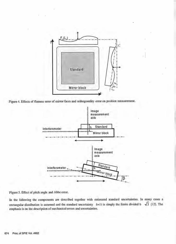
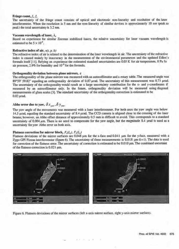


II
Publication II
B. Hemming, E. Ikonen, and M. Noorma, “Measurement of Aperture Diameters using an Optical Coordinate Measuring Machine”, International Journal of Optomechatronics, 1, 297 – 311 (2007). .
© 2007 Taylor & Francis, www.informaworld.com
Reprinted with permission.

Dow
nloa
ded
By:
[Hem
min
g, B
jörn
] At:
07:0
5 11
Sep
tem
ber 2
007
MEASUREMENT OF APERTURE AREAS USING ANOPTICAL COORDINATE MEASURING MACHINE
Bjorn Hemming,1 Erkki Ikonen,1,2 and Mart Noorma2,3
1Centre for Metrology and Accreditation (MIKES), Espoo, Finland2Metrology Research Institute, Helsinki University of Technology (TKK),Finland3University of Tartu, Tartu, Estonia
The use of an optical coordinate measuring machine (CMM) for the diameter measure-
ment of optical apertures is described. The traceability and mechanical stability of the aper-
ture areas are of importance for accurate photometric and radiometric measurements.
Detailed evaluation of the measurement uncertainty for the aperture diameter is presented.
High-accuracy mechanical CMM was used to confirm the validity of the optical CMM
results. The difference between the contact and non-contact measurement was 0.1mm for
the mean diameter result. If the required standard uncertainty for the mean diameter is
of the order of 1 mm, the optical CMM provides an efficient method for aperture area
measurements.
1. INTRODUCTION
Apertures are used in optical radiometry� to define a precisely known area ofan incoming radiation field in front of a detector. When the detector has a calibratedoptical power responsivity, the known aperture area allows to determine such quan-tities as illuminance or irradiance which describe optical power divided by area. Anideal aperture would have zero thickness in order to avoid shadowing of light raysentering in other than exactly perpendicular direction to the aperture plane. Reliablearea measurements of apertures with thin edges are especially important to primaryscale realizations, as otherwise it is not possible to get access to many essential radio-metric quantities.
The area of a nominally round aperture can be measured via determination ofits effective diameter. A straightforward method for diameter measurement is todetermine in different directions the largest distance between the edges of the aper-ture. The edges can be observed either by a microscope in an optical coordinate mea-suring machine (CMM) or by a physical contact in a mechanical CMM. The mainadvantage of the non-contact optical CMM method is that it does not damage thethin aperture edge. Furthermore, the measurement setup and alignment can be made
�Optical radiometry is the field of science which studies the measurement of electromagnetic radi-
ation, including visible light. Light is also measured using the techniques of photometry that deal with
brightness as perceived by the human eye.
Address correspondence to Bjorn Hemming, Centre for Metrology and Accreditation (MIKES),
Tekniikantie 1, FIN-02150 Espoo, Finland. E-mail: [email protected]
297
International Journal of Optomechatronics, 1: 297–311, 2007
Copyright # Taylor & Francis Group, LLC
ISSN: 1559-9612 print=1559-9620 online
DOI: 10.1080/15599610701548803

Dow
nloa
ded
By:
[Hem
min
g, B
jörn
] At:
07:0
5 11
Sep
tem
ber 2
007
relatively simple and it is easy to get a large number of diameter values in differentdirections. For mechanical contact measurements, utmost care is needed to protectthe thin aperture edge and to achieve correct alignment of the aperture plane relativeto the probe and probe motion. As a whole the contact measurement, per aperturediameter value, takes considerably longer time than the non-contact measurement.However, the measurement uncertainty of the contact method can be lower than thatof the non-contact method since in the latter case uncertainty is limited by the dif-ficulty in reliable determination of the aperture edge position in the microscopeimage.
Several contact (Martin et al. 1998) and non-contact (Fowler et al. 2000;Fowler et al. 1998; Lassila et al. 1997; Ikonen et al. 1998; Stock and Goebel 2000;Razet and Bastie 2006; Hartmann et al. 2000; Fowler and Litorja 2003) methodshave been used for measurement of aperture areas. Some non-contact methods(Lassila et al. 1997; Ikonen et al. 1998; Stock and Goebel 2000) can measure the areadirectly and are thus not sensitive to the shape of the apertures, but still require longmeasurement time. The reported relative standard measurement uncertainties aretypically 10�4 or less. However, even the best measurements of illuminance respon-sivity (Kohler et al. 2004) and spectral irradiance (Woolliams et al. 2006) haverelative standard uncertainties larger than 10�3. Therefore, in some cases an increasein measurement uncertainty for area is acceptable to improve the speed andefficiency of the aperture area measurements. Such an efficiency improvement isespecially important for a method (Kubarsepp et al. 2000) where more than ten sep-arate detectors (filter radiometers) are used to realize the spectral irradiance scale, aseach of these filter radiometers would need a dedicated 3-mm-diameter aperture withknown area. Another need for straightforward aperture area measurement comesfrom the study of mechanical stability of aperture diameter over time scales ofseveral months after the drilling. The non-contact optical CMM method is a goodcandidate for an efficient aperture area measurement. However, if the aperture areauncertainty starts to approach other uncertainty components in the spectralirradiance uncertainty budget, the need for a reliable uncertainty evaluation ofaperture diameter measurement with the optical CMM is emphasized.
During the last 10 years, coordinate measurement machines fitted with CCDcameras and machine vision software have been developed. These optical CMM’sare nowadays used widely especially in the electronic industry, because of their abil-ity for fast automated and accurate non-contact measurements. Typical claimed
NOMENCLATURE
D diameter
D mean diameter
k coverage factor
i, j, m index variables
n number of measured points
R, r Radius
x, y Cartesian coordinate
de error for measurement of D due to
optical parameters and edge sharpness
dr error for measurement of r due to edge
roundness of aperture
dx repeatability error for measurement of
x-coordinate
dy repeatability error for measurement of
y-coordinate
298 B. HEMMING ET AL.

Dow
nloa
ded
By:
[Hem
min
g, B
jörn
] At:
07:0
5 11
Sep
tem
ber 2
007 accuracies for optical CMM’s range from 0.8 mm to 6 mm. (Lazzari et al. 2004; Kivio
et al. 2004). These accuracies apply for one length measurement only, but with thesemachines complicated measurements, for example flatness, roundness, cylindricity,coaxiality, etc., are often carried out without knowledge of the task specified uncer-tainty. Moreover, the uncertainties written on manufacturers brochures are quiteseldom realistic and therefore the apparent estimated uncertainty of measurementsmay be far too small (Kivio et al. 2004).
Calculation of the measurement uncertainty for a real measurement task with aCMM is considered to be demanding mainly because there is a large number ofuncertainty sources and error components. Also several measurement strategiescan be used for the same task. Finally, the measurement task itself may include com-plex geometries or fitting algorithms (Chan et al. 1996). Additional practical dif-ficulty comes from the object to be measured with optical CMM: depending onthe selected light source and magnification, on the edge detection parameters, andon the edge itself, different results may be the outcome of measurements.
In this work, the use of optical CMM is studied as a candidate for an efficientaperture area measurement method. A detailed uncertainty analysis of optical CMMmeasurements is presented for the first time with uncertainty budgets for diametermeasurements to help for a better understanding of the measurement method.Especially, the measurement geometry and measurement strategy together with theeffects of the quality of the edges are explained. A specific purpose of the measure-ments was to study the stability of diameters of aluminium apertures over a timescale of six months after the drilling. After drilling the diameter might change, forexample due to oxidation or stresses in the material. The measured diameters showedonly minor changes comparable with the uncertainties in the measurements. Thestandard deviation for the measured diameter for one aperture was 35% or less ofthe standard uncertainty of the measurement. Measurements with a high-accuracymechanical CMM were used to confirm the validity of the optical CMM results.The optical method was found to provide a fast way for aperture area measurementsat an uncertainty level which is sufficient for most practical applications in photom-etry and radiometry and satisfies the needs of even the most accurate spectralirradiance measurements.
This article is organized as follows. Section 2 describes the measurement setupand Section 3 the measurement results. To confirm these non-contact measurements,measurements with contacting probe are made and described in Section 4. Beforeany conclusions can be drawn on the stability of the apertures or the suitability ofthe measurement method, an uncertainty budget is needed as described in Section5. In Section 6, conclusions on these two topics are presented.
2. OPTICAL APERTURE MEASUREMENTS
The optical diameter measurements were conducted using Mitutoyo Quickvi-sion Hyper CMM at the Centre for Metrology and Accreditation (MIKES) shownin Figure 1. Quickvision CMM is equipped with crystallized glass scale with the res-olution of 0.02 mm and thermal expansion coefficient of 0.08� 10�6=K. The bestspecified measurement uncertainty in one axis is 0.8 mm (Mitutoyo 2001). As shownin Figure 1, the object to be measured is placed on the motorized Y-table and the
MEASUREMENT OF APERTURE AREAS 299

Dow
nloa
ded
By:
[Hem
min
g, B
jörn
] At:
07:0
5 11
Sep
tem
ber 2
007
camera is moved using an X-stage and a vertical Z-stage. The instrument can be usedwith coaxial light and stage light. Stage light, also called contour illumination, uses alight source beneath the glass-made measuring table, and is useful when the object istoo reflective for coaxial light. The apertures have been made of aluminium with anominal diameter of 3 mm. Properties of the apertures are shown in Table 1. Toavoid a situation where both the new apertures and the CMM would be unstable,old, presumably stable apertures were also measured. The new apertures weremachined by conventional turning some days before the first measurement. If theaperture dimensions would be unstable immediately after turning, the difference inthe behaviour of new and old apertures would reveal this phenomenon.
A measurement program was made, where 120 points at the circumference ofthe apertures were measured and combined to a circle using the least-squares criteria.During the measurement X-Y-movements are made and a small part of the edge ofthe aperture is seen by the camera. Using the point measurement tool in the
Figure 1. A CMM used for the measurement of optical apertures. a) Schematic diagram and b) measure-
ment of apertures positioned using a fixture.
Table 1. Studied apertures and illumination used in the measurements. The percent
values indicate the fraction of full light intensity of the Quickvision Hyper
Aperture Age Coating Illumination (%)
HUT-1 new anodized Coaxial 80
HUT-2 old anodized Coaxial 80
HUT-3 new anodized Coaxial 80
HUT-4 new none Stage 30
HUT-5 new anodized Coaxial 80
HUT-6 old none Stage 30
HUT-7 old anodized Coaxial 80
HUT-8 new none Stage 30
HUT-9 new none Stage 30
HUT-10 old none Stage 30
300 B. HEMMING ET AL.

Dow
nloa
ded
By:
[Hem
min
g, B
jörn
] At:
07:0
5 11
Sep
tem
ber 2
007
Quickvision software, one point on the edge is measured. This sequence is repeatedat equal angle steps until a circle is completed. In addition to the calculated diameter,an out-of-roundness estimate was obtained from the circle-fitting function of theQVPak program of the CMM. Some raw measurement data of coordinates (x,y)were also saved for verification and plotting using Matlab (MathWorks, Inc.). Dur-ing the measurements the temperature of the CMM varied from 19.3�C to 20.4�C dueto the change of the ambient conditions. To ensure a good reproducibility and tominimize the influence of the systematic errors of the CMM, a fixture was used toposition the apertures (Figure 1).
3. MEASUREMENT RESULTS
The apertures were named HUT-1, HUT-2 . . . HUT-9. Results of the measure-ments are shown in Table 2. The variations in diameter for nine apertures werewithin 1.3 mm and for one old aperture, HUT-6, the maximum variation was1.6 mm. It is difficult to see any trend indicating a systematic change in any of theapertures. Figure 2 shows the results graphically for apertures HUT-8 and HUT-9, which were randomly selected to be measured also on day 3 and day 7.
Table 2. Results for mean diameters (in mm) of ten apertures for the period of six months
Day HUT-1 HUT-2 HUT-3 HUT-4 HUT-5 HUT-6 HUT-7 HUT-8 HUT-9 HUT-10
0 3.0082 3.0387 3.0063 3.0084 3.0025 3.0016 3.0336 3.0039 3.0076 2.9992
1 3.0085 3.0387 3.0057 3.0083 3.0034 3.0018 3.0333 3.0040 3.0070 2.9992
3 3.0039 3.0076
7 3.0037 3.0080
14 3.0079 3.0389 3.0054 3.0082 3.0033 3.0003 3.0332 3.0038 3.0081 2.9993
34 3.0083 3.0388 3.0056 3.0085 3.0034 3.0019 3.0330 3.0041 3.0074 2.9989
77 3.0085 3.0387 3.0056 3.0085 3.0032 3.0018 3.0334 3.0038 3.0083 2.9994
196 3.0080 3.0388 3.0052 3.0083 3.0036 3.0016 3.0332 3.0040 3.0083 2.9996
Figure 2. Measurement results of mean diameter for two apertures.
MEASUREMENT OF APERTURE AREAS 301

Dow
nloa
ded
By:
[Hem
min
g, B
jörn
] At:
07:0
5 11
Sep
tem
ber 2
007
In diameter measurements, the roundness plots are helpful when judging thequality of the data. From Figure 3, it can be seen that there are rather large localout-of-roundness variations in the measurement results. In Razet and Bastie(2006), this variation is referred to as edge scatter. The reason is probably actual geo-metrical form and roughness of the apertures combined with the effects of illumi-nation. These variations should be included in the uncertainty analysis asreproducibility errors because the position of the aperture cannot be exactly the samein every measurement.
4. COMPARISON TO THE RESULTS OBTAINED WITH MECHANICAL CMM
Verification measurements with a probing CMM Mitutoyo Legex were madefor the aperture HUT-1. The nominal maximum permissible error (MPEe error)defined in ISO 10360–2 (for this high-accuracy CMM is (0.35þL=1000) mm) whereL is the measured length in millimetres. The MPEe error is verified to be less than0.2 mm for measurement distances shorter than 100 mm using zerodur gauge blocks.The diameter of the probe was 2 mm and the measuring force was 0.045 N (Figure 4).Although the measurement force is quite small, the thin edges of optical aperturesmay be damaged by the mechanical measurement, and therefore this verificationusing probing CMM was done for only one aperture. The average measured diam-eter from 120 points was 3.0061 mm, as determined with mechanical CMM.
Because the probe is large compared to the roughness of the aperture, the mea-sured diameter is decreased by the contact error. During the measurement of eachpoint, the probe approaches the aperture in a radial movement starting approxi-mately from the aperture center. The first contact between the probe and the aper-ture is registered as a measurement point. Because there are roughness peaks on theaperture, most measurement points will be registered from these peaks. Thus, themechanical contact between the probe and aperture edge was simulated using optical
Figure 3. Roundness polar plot of aperture HUT-9 measured with 120 points: a) measured with 2000
points; b) dashed circles indicate 5 mm scale grid in the polar plot.
302 B. HEMMING ET AL.

Dow
nloa
ded
By:
[Hem
min
g, B
jörn
] At:
07:0
5 11
Sep
tem
ber 2
007
Figure 4. Basic geometry when measuring a 3-mm inner diameter using a 2-mm touch probe (scales in
millimetres).
Figure 5. Simulation of the contact between the aperture and the probe at several positions. The center of
the aperture is at (0, 0).
MEASUREMENT OF APERTURE AREAS 303

Dow
nloa
ded
By:
[Hem
min
g, B
jörn
] At:
07:0
5 11
Sep
tem
ber 2
007 CMM profile data. A Matlab script was written to adjust a radial offset to the
theoretical probe to match roughness peaks in a 2000-point aperture profile(Figure 5). The result of this simulation was an estimate of the contact error of1.1 mm in radius. The surface roughness of the probe was measured with a formand surface roughness measuring instrument. The roughness value Ra (arithmeticalmean roughness) is less than 0.05 mm, and therefore errors due to roughness effectsof the probe are negligible.
In addition, a force correction should be applied to the mechanical CMMresult. The force correction of �0.05 mm (in radius) was calculated from formulasfor elastic compression for the case of the sphere in contact with the internal cylinder(Puttock and Thwaite 1969). The depth of the cylindrical land in the aperture isabout 150 mm. After applying the force correction and the contact error correction,the resulting diameter is 3.0081 mm. The mean value of the measurements, conduc-ted with the optical CMM, was 3.0082 mm (Table 2), so there is good agreementbetween the results.
5. UNCERTAINTY ANALYSIS FOR MEASUREMENT OF MEAN DIAMETER
5.1. Auxiliary Measurement Results
The formal definition of uncertainty of a measurement is ‘‘parameter associa-ted with the result of a measurement, that characterizes the dispersion of the valuesthat could reasonably be attributed to the measurand’’ (GUM 2004). The compi-lation of the uncertainty budget requires additional studies of general stability ofthe instrument and repeatability and reproducibility of the measurements. In thisarticle, especially where the stability of the apertures has been studied, the reproduci-bility of the measurements and the stability of the optical CMM are critical. As pre-viously mentioned, a relative aperture area uncertainty of 10�3 would be sufficientfor most needs in photometry and radiometry. An aperture with a nominal diameterof 3 mm corresponds to a standard uncertainty of 1 mm for the mean diameter. In thefollowing, an uncertainty analysis is made to show that the accuracy of the measure-ments of the mean diameter is sufficient for these needs. Also, to make reliable con-clusions on the stability of the apertures a similar accuracy is needed.
The best measurement capability for Quickvision Hyper optical CMM is0.8 mm (k ¼ 2, k is the coverage factor with which the standard uncertainty is mul-tiplied to get an uncertainty at 95 % confidence level) in one axis for a short dis-tance measurement. There is also an additional length-dependent component ofuncertainty, but it is negligible in our case because the measured dimension issmall. This measurement capability has during recent years been verified by severalcalibrations and verification measurements of glass scales. It is assumed that theuncertainty consists mainly of the uncompensated error of the scale (0.6 mm,k ¼ 2) and of the repeatability error (0.5 mm, k ¼ 2). To ensure the accuracy in cur-rent measurements, additional verification measurements were performed using a50-mm glass scale positioned close to the area where the apertures were measured(Figure 6).
The position of each scale mark on the glass scale is taken as the middlebetween the two edges of a scale line. The reference values for the glass scale were
304 B. HEMMING ET AL.

Dow
nloa
ded
By:
[Hem
min
g, B
jörn
] At:
07:0
5 11
Sep
tem
ber 2
007
measured using the MIKES line-scale interferometer (Lassila et al. 1994). Theuncertainties of the reference values are almost negligible in this case (0.09 mm,k ¼ 2) and by repeating the measurement of this glass scale at the opticalCMM, the error of the CMM scale and repeatability error can be evaluated. Aver-aging a large number of measurements (point by point) shows a systematic contri-bution below �0.6 mm (Figure 7), and from these measurements the standarddeviation for each point was 0.2 mm. The systematic contribution is assumed tocome from the error of the CMM scale. These results are in agreement with theabove mentioned division of the measurement uncertainty into a component of0.6 mm for the CMM scale and 0.5 mm for the CMM repeatability (at coveragefactor k ¼ 2).
Figure 7. Difference between the values measured with MIKES line scale interferometer and Mitutoyo
Quickvision in the direction of the a) x-axis and b) y-axis.
Figure 6. Verification measurements using a reference glass scale in the same position as the aperture.
MEASUREMENT OF APERTURE AREAS 305

Dow
nloa
ded
By:
[Hem
min
g, B
jörn
] At:
07:0
5 11
Sep
tem
ber 2
007 5.2. The Simplified Measurement Model
When estimating measurement uncertainty according to the guidelines pre-sented in GUM (1993), the first task is to write a formula for the measurementmodel. The basic measurement model for a simple two-point diameter (D) measure-ment in the direction of the x-axis is
D ¼ x2 � x1 þ dx1 þ dx2 þ dr1 þ dr2 þ de; ð1Þ
where x1 and x2 are the first and second measured coordinates, dx1 and dx2 are therepeatability errors, dr1 and dr2 are the errors from edges of the measured object(roundness errors), and de is the edge detection error for diameter. The errors dr1
and dr2 are due to roundness errors in the horizontal plane of the aperture, andthe edge detection error de depends on user selected illumination, focus and sharp-ness of the edge. In one measurement, parameter D is calculated only from the esti-mates x1 and x2 but the measurement model contains also contributions from errors.The principle of two-point measurement is shown in Figure 8.
The measurements were actually made of 120 points and the resulting diametercan be interpreted as the mean D of 60 diameter measurements. Therefore, the effectof the repeatability error (dx1 and dx2) and the roundness error, including roughness,(dr1 and dr2) should be decreased by the factor 1=
p60. The position of the found
edge depends on user selected illumination, focus, and sharpness of the edge. Therelated error de is of systematic type and cannot be reduced by averaging and thusthe measurement model of repeated measurements is rewritten as
D ¼ 1
60
X60
m¼1
½x2;m � x1;m þ dx1;m þ dx2;m þ dr1;m þ dr2;m� þ de: ð2Þ
The contribution of the uncertainty component de was studied by changingillumination. It should be noted that this uncertainty component is much morecomplicated in the detection of the aperture edge than, for example, in the detection
Figure 8. a) Two-point measurement of diameter and b) multi-point measurement of diameter.
306 B. HEMMING ET AL.

Dow
nloa
ded
By:
[Hem
min
g, B
jörn
] At:
07:0
5 11
Sep
tem
ber 2
007 of the scale mark distances on the reference glass scale. When using stage light, the
aperture is between the camera and the light source. The aperture appears as darkarea and at the edge there is a transition of illuminance level. When illuminationis increased, the amount of light coming to the CCD camera increases, and finallythe whole image would be saturated to bright signal. Before this happens, it canbe seen that the transition range between dark and bright seems to move away fromthe bright area. This phenomenon increases the diameter of bright holes, anddecreases the width of dark lines on glass scales. However, the distance betweenthe centers of the scale marks remains unaffected when the position of the scalemarks is taken as the center of the dark lines.
One matte aperture (HUT-1) and one bright aperture (HUT-9) were measuredwith a large range of combinations of coaxial and stage light. The standard deviationof obtained diameters was 0.86 mm for the matte aperture and 0.61 mm for the brightaperture. The results for the illumination experiment for the matte aperture are givenin Table 3. It is seen that strong illumination (50% column for stage light) leads toroughly 4 mm larger diameter than with moderate or zero stage light. However, theuser also receives a ‘‘saturation warning’’ so these diameter results are excluded fromthe data when calculating the above mentioned standard deviations. The standarduncertainty related to de is estimated to be 1 mm, from Table 3. The value is con-servative and rounded upwards to include the contribution of effects which cannot be addressed by varying illumination conditions.
Next, the error of roundness type is dealt with. When the diameter measure-ment was immediately repeated, the variation in results was typically only 0.1 mm.However, if the aperture was removed and measured again, with 120 points, in aslightly different position, the change in diameter was typically 0.1 mm–0.5 mm, indi-cating a considerable reproducibility error. The reason is seen in Figure 3; i.e., theedge appears to be rough and uneven. The roundness error was typically with-in�4 mm. The related standard uncertainty, assuming a rectangular distribution, isdr1 ¼ dr2 ¼ (4 mm)=
p3 ¼ 2.31 mm (GUM 1993).
Table 3. Effects of illumination on the diameter of a matte aperture (HUT-1), in
millimetres. The illumination selected for measurements of matte apertures was
80% for coaxial light and 0% for stage light
Stage light illumination magnitude [%]Coaxial light illumination
magnitude [%] 0 20 30 40 50
0 3.0071 3.0074 3.0084 3.0115
10
20 3.0073 3.0075 3.0084 3.0115
30
40
50 3.0064 3.0076 3.0076 3.0087 3.0116
60 3.008
70 3.0081
80 3.0079 3.0079 3.0076 3.0096 3.0121
90 3.008
100 3.008 3.008 3.0084 3.0105 3.0128
MEASUREMENT OF APERTURE AREAS 307

Dow
nloa
ded
By:
[Hem
min
g, B
jörn
] At:
07:0
5 11
Sep
tem
ber 2
007
The uncertainty budget for the simplified model is shown in Table 4. Theexpanded measurement uncertainty for the average diameter is 2.33 mm (k ¼ 2)and the corresponding relative standard uncertainty is 8� 10�4 for a 3-mm-diameteraperture.
For analysis of the stability of the apertures, the uncertainty component de iszero assuming no changes in ambient illumination or ageing of light bulbs in theoptical CMM. It may also be assumed that the effect of the uncompensated system-atic error of the CMM scales can be neglected in a reproducibility analysis. Withthese assumptions, the expanded diameter uncertainty of Table 4 is reduced to0.85 mm (k ¼ 2) for analysis of temporal drift of the aperture diameters. From datain Table 2, it can be calculated that the standard deviation of one measured aperturewas on the average 0.29 mm.
During the measurement series the variations of temperature were lessthan �0.55 K. The thermal expansion of the glass scale of the optical CMM is verylow (0.08� 10�6=K) and the dimension of the aperture is small. Therefore, variationin the average temperature of the measurement is not significant and is not includedin the uncertainty analysis. Another temperature-related error source is the rapidchange of temperature of the CMM body structure during one measurement. Inan experiment using a 2000-W heat-fan warming at one side of the CMM, the sen-sitivity of 0.6 mm=K was found for the diameter measurement. During the measure-ments, the slow changes of temperature in the measurement laboratory can thereforebe neglected.
5.3. Measurement Model for Actual Geometry and Monte-CarloSimulations
The measurement model of Eq. (2) contains only x-axis components andis therefore not entirely correct. The next step is to rewrite the equation tomatch the actual measurement of n points giving n=2 diameters (Figure 8) alongthe circumference.
Di ¼ Ri þ Rn=2þi þ de; i ¼ 1 . . . n=2; ð3Þ
Table 4. Uncertainty budget for an averaged diameter measurement
Uncertainty Component Standard uncertainty [mm]
x1 Uncompensated error of CMM scales 0.30
dx1=p
60 Repeatability for one point 0.03
dr1=p
60 Local error of edge of measured object 0.30
x2 Uncompensated error of CMM scales 0.30
dx2=p
60 Repeatability for one point 0.03
dr2=p
60 Local error of edge of measured object 0.30
de Edge detection 1.00
Combined standard uncertainty (k ¼ 1) 1.17
D Expanded uncertainty (k ¼ 2) 2.33
308 B. HEMMING ET AL.

Dow
nloa
ded
By:
[Hem
min
g, B
jörn
] At:
07:0
5 11
Sep
tem
ber 2
007 where
Rj ¼ffiffiffiffiffiffiffiffiffiffiffiffiffiffiffiffiffiffiffiffiffiffiffiffiffiffiffiffiffiffiffiffiffiffiffiffiffiffiffiffiffiffiffiffiffiffiffiffiffiðxj þ dxjÞ2 þ ðyj þ dyjÞ2
qþ drj; j ¼ 1::n ð4Þ
Equation (3) can be interpreted as the sum of 60 pairs of opposite 120 radii giving 60diameters.
The Monte-Carlo method is clearly useful in uncertainty analysis in metrology(Brizzard et al. 2005; Mudronja et al. 2003). Briefly, the idea is to simulate themeasurement model M times using random numbers. According to the law of largenumbers the distribution of the M outputs of the model converge to the actual dis-tribution if the input distributions are reasonably correct. The systematic part ofthe uncompensated error of the CMM is simulated by a sine function with anamplitude of 0.5 mm, and the repeatability of the CMM is simulated by a normaldistribution. The edge detection and local error of the measured object were alsosimulated by normal distributions based on standard uncertainties described inthe previous sections.
The measurement model was implemented in Matlab using random numbersfrom these distributions. The measurement software of the CMM uses least-squarescircle fitting, and least-squares circle fitting was also included in the measurementmodel in Matlab. Finally, the standard deviation and the 95% confidence intervalare calculated from the distribution.
The 95% coverage interval for diameter based on 100,000 simulations from thedistribution of the simulated values is 2.1 mm (Figure 9). This is slightly less than theresult in Table 4 (2.33 mm). A major advantage with the Monte-Carlo approach is thecorrect simulation of the measurement strategy, and now the number of measure-ment points n can be easily changed in the model. Table 5 shows that if the numberof measurement points in the model is changed from 120 to 2 points, the expandeduncertainty from the simulation is 6.7 mm which is close to the value 6.6 mm obtained
Figure 9. Distribution of the simulated diameter measurements using a) 2 points and b) 120 points.
MEASUREMENT OF APERTURE AREAS 309

Dow
nloa
ded
By:
[Hem
min
g, B
jörn
] At:
07:0
5 11
Sep
tem
ber 2
007
for 2-point measurement with the values in Table 4. The reproducibility according tothe simulation with 120 points is 0.8 mm, slightly less than the result of 1.2 mm in theprevious section.
6. CONCLUSION
The optical CMM was found to be a suitable device for the diameter measure-ment of optical apertures. The repeatability of the aperture measurement results isvery good with a typical standard deviation of 0.2 mm for a point and 0.1 mm forthe mean diameter (average from 120 points). The reproducibility, affected byroundness error of the specimen, temperature and ambient light, is much larger,about 1 mm (k ¼ 2) for the diameter obtained as an average of 120 points.
Although some of the measured changes in the aperture diameter are close tothe estimated reproducibility of the measurement, the nature of these variations sug-gests that there has not been any systematic growth or shrink, for example, from oxi-dation or stresses of the apertures. Therefore, it appears that the aperture diametershave been stable during the studied period.
Earlier experiences with the optical CMM and the comparisons with the prob-ing CMM have shown a large operator-dependent factor which probably can betraced to illumination selections. The expanded measurement uncertainty for averagediameter is 2.33 mm (k ¼ 2). However, in this study the measurements with the prob-ing CMM appear to confirm the optical CMM’s result very well. The conclusion isthat if the required relative uncertainty in the aperture area is of the order of 0.1%the optical CMM used in this study is useful for aperture diameter measurements.
REFERENCES
Brizard, M., M. Megharfi, and C. Verdier. 2005. Absolute falling-ball viscometer: Evaluationof measurement uncertainty. Metrologia 42(4):298–303.
Chan, F. M., T. King, and K. Stout. 1996. The influence of sampling strategy on a circularfeature in coordinate measurements. Measurement 19(2):73–81.
Fowler, Joel, R. Saunders, and Albert Parr. 2000. Summary of high-accuracy aperture-areameasurement capabilities at the NIST. Metrologia 37(5):621–623.
Table 5. Measurement uncertainty and reproducibility using Monte-
Carlo simulation
n
Uncertainty at 95%
confidence level, [mm]
Reproducibility at 95%
confidence level [mm]
2 6.7 6.4
4 4.9 4.5
12 3.3 2.6
36 2.5 1.5
60 2.3 1.2
120 2.1 0.8
360 2.0 0.5
310 B. HEMMING ET AL.

Dow
nloa
ded
By:
[Hem
min
g, B
jörn
] At:
07:0
5 11
Sep
tem
ber 2
007
Fowler, Joel, R. Durvasula, and Albert Parr. 1998. High-accuracy aperture-area measurementfacilities at the National Institute of Standards and Technology. Metrologia 35(4):497–500.
Fowler, Joel and Maritoni Litorja. 2003. Geometric area measurements of circular aperturesfor radiometry at NIST 2003. Metrologia 40(1):S9–S12.
Guide to the expression of uncertainty in measurement (GUM). 2004. Supplement 1: Numeri-cal methods for the propagation of distributions using a Monte Carlo Method (ISO),draft.
Hartmann, Juergen, Joachim Fischer, and Joachim Seidel. 2000. A non-contact technique pro-viding improved accuracy in area measurements of radiometric apertures. Metrologia37(5):637–640.
International Organization for Standardization (ISO). 1993. Guide to the expression on uncer-tainty in measurement (GUM); Geneva.
Kivio, Heli, Tero Ristonen, Jaakko Salmi, and Heikki Tikka. 2004. Comparison of opticalCMMs. VDI=VDE-GMA, Proceedings of the 8th International Symposium on measure-ment and quality control in production. 145–156.
Kohler, Rainer, Michael Stock, and C. Garreau. 2004. Final report on the international com-parison of luminous responsivity CCPR-K3.b. Metrologia 41(1A) Tech Suppl.:1–30.
Kubarsepp, Toomas, Petri Karha, Manoocheri Farshid, Nevas Saulius, Ylianttila Lasse, andIkonen Erkki. 2000. Spectral irradiance measurements of tungsten lamps with filter radio-meters in the spectral range 290 nm to 900 nm. Metrologia 37(4):305–312.
Ikonen, Erkki, Pasi Toivanen, and Antti Lassila. 1998. A new optical method for high-accuracy determination of aperture area. Metrologia 35(4):369–372.
Lassila, Antti, Pasi Toivanen, and Erkki Ikonen. 1997. An optical method for direct determi-nation of the radiometric aperture area at high accuracy. Meas Sci Technol 8(9):973–977.
Lassila, Antti, Erkki Ikonen, and Kari Riski. 1994. Interferometer for calibration of graduatedline scales with a moving CCD camera as a line detector. Applied Optics 33(16):3600–3603.
Lazzari, Annarita and Gaetano Iuculano. 2004. Evaluation of the uncertainty of anoptical machine with a vision system for contact-less three-dimensional measurement.Measurement 36(3–4):215–231.
Martin, John, N. Fox, N. Harrison, B. Shipp, and M. Anklin. 1998. Determination and com-parisons of aperture areas using geometric and radiometric techniques. Metrologia35(4):461–464.
Mitutoyo America Corporation. 2001. Hyper quick vision brochure, bulletin no 1510. Paramus,NJ: Mitutoyo America Corporation.
Mudronja, Vedran, Biserka Runje, and Srdan Medic. 2003. Examples of applying MonteCarlo simulations in the field of measurement uncertainties of the standard of length.Proceedings of the XVII IMEKO World Congress, 1130–1134.
Puttock, M. and E. Thwaite. 1969. Elastic Compression of Spheres and Cylinders at Point andLine Contact, National Standards Laboratory Technical Paper No. 25, Division ofAppled Phyics, National Standards Laboratory, Commonwealth Scientific and IndustrialResearch Organization (CSIRO), University Grounds, Chippendale, New South Wales,Australia.
Razet, Annick and Jean Bastie. 2006. Uncertainty evaluation in non-contact aperture areameasurements. Metrologia 43(5):361–366.
Stock, Michael and Roland Goebel. 2000. Practical aspects of aperture-area measurements bysuperposition of Gaussian laser beams. Metrologia 37(5):633–636.
Woolliams, Emma R., Nigel P. Fox, Maurice G. Cox, Peter M. Harris, and Neil J. Harrison.2006. Final report on CCPR K1-a: Spectral irradiance from 250 nm to 2500 nm.Metrologia 43(1A) Tech Suppl.:1–396.
MEASUREMENT OF APERTURE AREAS 311

III
Publication III
B. Hemming and H. Lehto, “Calibration of Dial Indicators using Machine Vision,” Meas. Sci. Technol. 13, 45-49 (2002). http://www.iop.org/EJ/abstract/0957-0233/13/1/306/ © 2002 IOP, http://www.iop.org/EJ/journal/MST
Reprinted with permission.
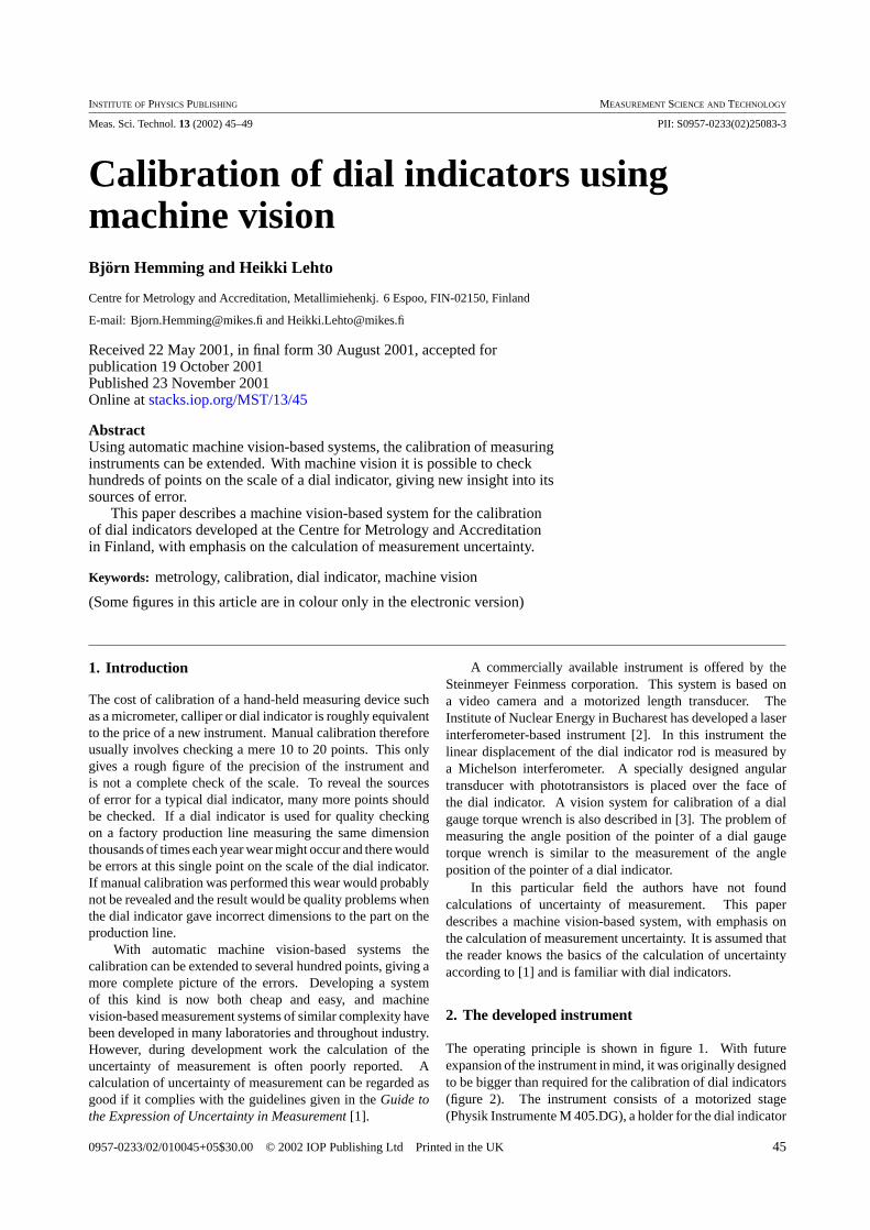
INSTITUTE OF PHYSICS PUBLISHING MEASUREMENT SCIENCE AND TECHNOLOGY
Meas. Sci. Technol. 13 (2002) 45–49 PII: S0957-0233(02)25083-3
Calibration of dial indicators usingmachine visionBjorn Hemming and Heikki Lehto
Centre for Metrology and Accreditation, Metallimiehenkj. 6 Espoo, FIN-02150, Finland
E-mail: [email protected] and [email protected]
Received 22 May 2001, in final form 30 August 2001, accepted forpublication 19 October 2001Published 23 November 2001Online at stacks.iop.org/MST/13/45
AbstractUsing automatic machine vision-based systems, the calibration of measuringinstruments can be extended. With machine vision it is possible to checkhundreds of points on the scale of a dial indicator, giving new insight into itssources of error.
This paper describes a machine vision-based system for the calibrationof dial indicators developed at the Centre for Metrology and Accreditationin Finland, with emphasis on the calculation of measurement uncertainty.
Keywords: metrology, calibration, dial indicator, machine vision
(Some figures in this article are in colour only in the electronic version)
1. Introduction
The cost of calibration of a hand-held measuring device suchas a micrometer, calliper or dial indicator is roughly equivalentto the price of a new instrument. Manual calibration thereforeusually involves checking a mere 10 to 20 points. This onlygives a rough figure of the precision of the instrument andis not a complete check of the scale. To reveal the sourcesof error for a typical dial indicator, many more points shouldbe checked. If a dial indicator is used for quality checkingon a factory production line measuring the same dimensionthousands of times each year wear might occur and there wouldbe errors at this single point on the scale of the dial indicator.If manual calibration was performed this wear would probablynot be revealed and the result would be quality problems whenthe dial indicator gave incorrect dimensions to the part on theproduction line.
With automatic machine vision-based systems thecalibration can be extended to several hundred points, giving amore complete picture of the errors. Developing a systemof this kind is now both cheap and easy, and machinevision-based measurement systems of similar complexity havebeen developed in many laboratories and throughout industry.However, during development work the calculation of theuncertainty of measurement is often poorly reported. Acalculation of uncertainty of measurement can be regarded asgood if it complies with the guidelines given in the Guide tothe Expression of Uncertainty in Measurement [1].
A commercially available instrument is offered by theSteinmeyer Feinmess corporation. This system is based ona video camera and a motorized length transducer. TheInstitute of Nuclear Energy in Bucharest has developed a laserinterferometer-based instrument [2]. In this instrument thelinear displacement of the dial indicator rod is measured bya Michelson interferometer. A specially designed angulartransducer with phototransistors is placed over the face ofthe dial indicator. A vision system for calibration of a dialgauge torque wrench is also described in [3]. The problem ofmeasuring the angle position of the pointer of a dial gaugetorque wrench is similar to the measurement of the angleposition of the pointer of a dial indicator.
In this particular field the authors have not foundcalculations of uncertainty of measurement. This paperdescribes a machine vision-based system, with emphasis onthe calculation of measurement uncertainty. It is assumed thatthe reader knows the basics of the calculation of uncertaintyaccording to [1] and is familiar with dial indicators.
2. The developed instrument
The operating principle is shown in figure 1. With futureexpansion of the instrument in mind, it was originally designedto be bigger than required for the calibration of dial indicators(figure 2). The instrument consists of a motorized stage(Physik Instrumente M 405.DG), a holder for the dial indicator
0957-0233/02/010045+05$30.00 © 2002 IOP Publishing Ltd Printed in the UK 45

B Hemming and H Lehto
Figure 1. Operating principle of the instrument.
Figure 2. The developed instrument.
and two length transducers (Heidenhein MT25), and a height-adjustable red LED ring light (CSI FPR-100) together with aCCD camera (figure 3). A fibre ring light was also tested butreflections occurred on the glass of the dial indicator undertest. The ring light has 65 LEDs, and by adjusting it to theappropriate height there are almost no shadows or glints on thedial indicator.
A CCIR standard camera (Cohu 4910) with resolution752 × 582 was installed with a 50 mm Rainbow G50 lens.The position of the stage was measured by the two lengthtransducers and their average used as a position reference toeliminate the Abbe error. The software was written with theVisual Basic 6 development tool in Windows NT 4 using theMatrox ActiveMIL library.
Figure 3. The ring light and length transducers (photoE Makkonen).
Figure 4. Subtraction gives a pixel by pixel difference between theimages.
3. Image aqcuisition and segmentation
The image is digitized at the frame grabber (Matrox Meteor II)to a resolution of 768 × 576. In order to exclude unwantedfeatures from the image a simple method also used in [3] was
46

Calibration of dial indicators using machine vision
Figure 5. Measurement of the scale marks on the dial.
implemented. Removal of the static background comprisingthe dial is done by the subtraction of two images of the dial(figure 4). Since the pointers are the only moving part of thedial, subtraction results in the removal of everything in theimages except the pointers [3]. The resulting image is of goodquality and it was felt that thresholding would not increase theedge-finding precision. It is assumed that the large pointer ison its right lap, making it unnecessary to measure the positionof the small pointer. The position of the outer part of the largepointer is found using the edge-finding functions of the MILlibrary. The centre of the pointer is given by the user mouse-clicking on a pair of points on the image of the dial indicatorassumed to be symmetrical to the centre. The angle of thelarge pointer is calculated from the line crossing the assumedstatic centre and the established position of the outer part ofthe pointer. Calibration of the scale marks on the dial is alsoimplemented in the software as a separate task (figure 5).
Figure 6. Error curve of a dial indicator measured manually and using the developed machine vision system with four repetitions.
4. Results
The first test on the system was performed with an almostnew Compac dial indicator with scale marks at 0.01 mmdivision. The error curve of the dial indicator in figure 6 showsthat to get a complete picture of the errors several hundredpoints need to be measured. Figure 6 shows an oscillatingpattern in the error curve. This frequency information canbe further studied by calculating the spectrum using a Fouriertransform (figure 7). In signal analysis the spectra are usuallyplotted as a function of frequency, but in length metrologythe wavelength is more informative. The spectrum revealsharmonics at wavelengths of 0.625, 1 and 12.5 mm whichpossibly correspond to respective sources of error in themechanism of the dial indicator.
5. Uncertainty budget
The principle of the calculation of uncertainty of measurementis described in [1] and a complete worked example for gaugeblocks is described in [5]. The error sources should beevaluated from measurements, experiment, data sheets orexperience. The error �L of a 0.01 mm division dial indicatoris obtained from the relationship
�L = Lp − �Lk − Lref (1)
where Lp is the measured pointer position of the dial indicator,�Lk is the measured error of the kth scale mark on the dialindicator and Lref is the reference position.
The pointer position Lp of a 0.01 mm division dialindicator is obtained from the relationship
Lp = 1
2πtan−1
[xc − xm
ym − yc
]+ δLα (2)
where xm, ym is the position of the indicator tip found by
47

B Hemming and H Lehto
Table 1. Uncertainty budget for the pointer of a 0.01 mm graduated dial indicator over a movement of 10 mm. Ideally the angle of theindicator should be 0◦, but in this example the position of the indicator is found half a pixel away at 365.5, 166.
Uncertainty Standard Degrees ofcomponent Estimate uncertainty Distribution Sensitivity coeff. Uncertainty freedom
δLα 0 1.0◦ Normal 0.01 µm/◦ 0.01 µm 8xc 366 pixels 0.23 pixel Rectang. 0.94 µm/pixel 0.22 µm 7yc 311 pixels 0.23 pixel Rectang. 0.94 µm/pixel 0.22 µm 7xm 365.5 pixels 0.34 pixel Rectang. 0.94 µm/pixel 0.32 µm 6ym 116 pixels 0.34 pixel Rectang. 0.94 µm/pixel 0.32 µm 6
Lp 0.4 µm 0.55 µm 22
Table 2. Uncertainty budget for the scale mark 0.0 mm (k = 1) on the dial of a 0.01 mm graduated dial indicator. Ideally the mark shouldbe 0◦, but in this example the position of the indicator is found 0.2 pixel away at 365.8, 81.
Uncertainty Standard Degrees ofcomponent Estimate uncertainty Distribution Sensitivity coeff. Uncertainty freedom
k 1 — — — — — — —δLα 0 1.0◦ Normal 0.01 µm/◦ 0.01 µm 8xc 366 pixels 0.23 pixel Rectang. 0.66 µm/pixel 0.15 µm 7yc 311 pixels 0.23 pixel Rectang. 0.66 µm/pixel 0.15 µm 7xk 365.8 pixels 0.34 pixel Rectang. 0.66 µm/pixel 0.22 µm 7yk 81 pixels 0.34 pixel Rectang. 0.66 µm/pixel 0.22 µm 7
�Lk −0.1 µm 0.38 µm 25
Table 3. Uncertainty budget for the reference position together with the mechanical error sources.
Uncertainty Standard Degrees ofcomponent Estimate uncertainty Distribution Sensitivity coeff. Uncertainty freedom
δ�L 0 mm 0.3 µm Normal 1 0.30 µm 5Li 10 mm 0.24 µm Rectang. 1 0.24 µm 5δLβ 0 0.5◦ Normal 0.04 µm/◦ 0.02 µm 8δLT 0 K 1 K Normal 0.12 µm/K 0.12 µm 5
Lref 10 mm 0.40 µm 12
Table 4. Uncertainty budget for the measurement error of a 0.01 mm graduated dial indicator over a movement of 10 mm. The number oflaps of the pointer are not counted and Lref = 0 mm is used instead of 10 mm.
Uncertainty Standard Degrees ofcomponent Estimate uncertainty Distribution Sensitivity coeff. Uncertainty freedom
Lp −0.4 µm 0.55 µm Normal 1 0.55 µm 22�Lk 0.1 µm 0.38 µm Normal 1 0.38 µm 25Lref 0 µm 0.40 µm Normal 1 0.40 µm 12
�L −0.4 µm 0.78 µm 53
the edge finding algorithm, xc, yc is the estimated centre ofthe indicator and δLα are the vertical plane alignment cosineerrors.
The error �Lk of the scale marks noted as k = 1, 2 . . . 100is obtained from the relationship
�Lk = 1
2πtan−1
[xc − xk
yk − yc
]− 0.01k + δLα (3)
where xk, yk is the position of the kth scale mark found bythe edge-finding algorithm, xc, yc is the estimated centreof indicator and δLα are the vertical plane alignment cosineerrors.
The errors in the camera and lens are about ±0.3 pixel inthe x and y directions measured with the calibration grid [4].The standard uncertainty, assuming a rectangular distribution,is
0.3 pixel√3
= 0.18 pixel.
The error for the edge-finding algorithm for the pointer isestimated to be ±0.5 pixel and the standard uncertainty is
0.5 pixel√3
= 0.29 pixel.
Adding the camera and lens errors gives
δxm = δym =√
0.292 + 0.182 = 0.34 pixel.
To estimate the centre of the indicator it is assumed that theuser gives two pairs (divisor
√4) of points, each having an
uncertainty of ±0.5 pixel. The standard uncertainty is
0.5 pixel√4√
3= 0.14 pixel.
Adding the camera and lens errors gives
δxc = δyc =√
0.142 + 0.182 = 0.23 pixel.
48

Calibration of dial indicators using machine vision
Figure 7. Spectrum of the error curve in figure 6 (repetition 1) as afunction of wavelength.
The reference position Lref together with the mechanical errorsources is
Lref = Li + δLT + δ�L + δLβ (4)
where Li is the average reading of the two length transducersused as reference, δLβ are the horizontal plane alignmentcosine errors, δ�L is the repeatability of the dial indicator andδLT is the error due to thermal expansion caused by heatingfrom the ring light.
The calibration result for the length transducers givesa ±0.6 µm uncertainty for each length transducer for a10 mm length. The distribution of the error is assumed tobe rectangular (divisor
√3) and the average reading of the two
transducers (divisor√
2) is used. The standard uncertainty is
δLi = 0.6 µm√2√
3= 0.24 µm.
The standard uncertainty for alignment cosine errors isestimated to be 0.5◦ for horizontal errors and 1◦ for verticalerrors. The vertical is interpreted as squareness between thedial indicator and the optical axis of the camera and lens. Thestandard uncertainty for the repeatability of a good 0.01 mmgraduated dial indicator is estimated to be 0.3 µm. Thestandard uncertainty for warming is estimated to be 1 K whichcorresponds to thermal expansion of 0.12 µm for a length of10 mm.
An example of calculation of the uncertainty for themeasured error of the dial indicator at one point for eachgroup of error sources is shown in tables 1–3. The totalcombined uncertainty is shown in table 4. The tables also givevalues for the degrees of freedom. The degrees of freedomνi are estimated according to the relative uncertainty in theuncertainty �u/u:
νi = 1
2
[�u(xi)
u(xi)
]−2
. (5)
The degrees of freedom are combined using the Welsh–Satterthwaite formula [1]:
νeff = u4c(y)∑N
i=1u4
i (y)
νi
. (6)
To express the expanded uncertainty at the 95% confidencelevel the combined standard deviation (table 4) is multipliedby 2.01 (t-distribution for n = 53 and 0.95) giving ±1.57 µm.
When a dial indicator is calibrated manually, theuncertainty of the reading and interpretation of the pointer isof the same order as that obtained with the developed machinevision system.
6. Conclusion
Using machine vision in a normal routine calibration makesit possible to check hundreds of points on the scale of a dialindicator. This extension of the calibration gives new insightinto the errors and error sources of the dial indicator. Thefrequency information of the error curve can also be studiedby calculating the Fourier transform.
Questions of measurement error and uncertainty are oftenignored. There are some natural reasons for this: if a newmeasurement system has been developed and it seems to work,why should anyone exceed the budget and timetable by makingtests that might show that the instrument is not within thespecification?
It is the view of the authors that the uncertainty budgetis part of the design process for a of a measuring instrument,just like the drawings. Real confidence in a machine vision-based measuring instrument is only achieved by systematicdocumentation and calculation of the uncertainties as shownin this paper.
References
[1] ISO 1993 Guide to the Expression of Uncertainty inMeasurement (Geneva: International Organization forStandardization)
[2] Sporea D G and Miron N 1996 Dial indicators checking-up bylaser interferometry Rev. Sci. Instrum. 67 612–14
[3] Aggarwal N, Doiron T and Sanghera P S Vision system for dialgage torque wrench calibration Proc. SPIE 2063 77–85
[4] Tsai R Y 1987 A versatile camera calibration technique forhigh-accuracy 3D machine vision metrology usingoff-the-shelf TV cameras and lenses IEEE J. Robot. Autom. 3323–44
[5] Decker J E, Ulrich A and Pekelsky J R 1998 Uncertainty ofgauge block calibration by mechanical comparison: aworked example for gauge blocks of dissimilar materialsProc. SPIE 3477 225–46
49

IV
Publication IV
B. Hemming, A. Fagerholm, and A. Lassila, “High-accuracy Automatic Machine Vision Based Calibration of Micrometers”, Meas. Sci. Technol. 18, 1655-1660 (2007).
http://www.iop.org/EJ/abstract/0957-0233/18/5/058/
©2007 IOP, http://www.iop.org/EJ/journal/MST
Reprinted with permission.

IOP PUBLISHING MEASUREMENT SCIENCE AND TECHNOLOGY
Meas. Sci. Technol. 18 (2007) 1655–1660 doi:10.1088/0957-0233/18/5/058
High-accuracy automatic machine visionbased calibration of micrometersB Hemming, A Fagerlund and A Lassila
Centre for Metrology and Accreditation, Tekniikantie 1, Espoo, FIN-02150, Finland
E-mail: [email protected]
Received 12 December 2006, in final form 7 March 2007Published 13 April 2007Online at stacks.iop.org/MST/18/1655
AbstractThe calibration of simple handheld instruments is often more expensive thanthe price of a new device. Therefore, the amount of manual labour is kept ata minimum in order to keep the price of calibration at a tolerable level. Thisalso means that only a few points of e.g. a length scale can be checked. Byusing automatic machine vision based systems, the calibration ofmeasurement instruments can be done faster and more thoroughly. In orderto study the possibilities of machine vision automation for volumecalibration tasks a set-up for micrometer calibration was constructed atCentre for Metrology and Accreditation (MIKES). With the developedautomated machine vision system it is possible to check hundreds of pointson the scale of a micrometer, giving new insight into error sources of themicrometer screw. The attained uncertainty is at the same level ascalibration with gauge blocks according to ISO 3611.
Keywords: metrology, calibration, micrometer, machine vision
1. Introduction
The manual calibration of a micrometer calliper according toIS0 3611 is done by using ten gauge blocks [1]. This givesonly a rough figure of the accuracy of the instrument and isnot a complete check of the scale. To reveal the error sourcesof a typical micrometer, many more points should be checked.Possible error sources are zero setting error, form error on themeasuring faces, pitch error and nonlinearities in the screw,location errors or bad quality of graduation lines on the thimbleand variations in the measuring force.
During recent years many measurement tasks both inindustry and in laboratories have been automated usingmachine vision. With automatic machine vision based systemsthe calibration can be extended to several hundred points,giving a more complete picture of the errors.
Two important matters in measurements and calibrationsare traceability and measurement uncertainty. The complexityof measurement uncertainty increases along with thecomplexity of the measurement equipment. Accuracy andmeasurement uncertainty in machine vision were previouslydiscussed thoroughly in papers [2–4], but the presentationdiffers from the approach in the Guide to the Expression ofUncertainty in Measurement (GUM) [5].
In a previous paper the author has presented equipmentfor automatic calibration of dial indictors [6]. In this paperthe updating of that equipment into a calibration devicefor micrometers is described. Detailed uncertainty analysisfollowing recommendations of GUM is also given.
2. The developed instrument
The calibration of a micrometer according to ISO3611 includes flatness and parallellity inspection of themeasurement surfaces, measurement of the measurementforce of the micrometer, checking the zero adjustment andmeasurement of the micrometer scale. The measurement ofmicrometer screw errors and measurement of force can bedone with the developed instrument.
The instrument consists of two motorized stages, a lengthtransducer and a red LED ring light together with a CCDcamera (figures 1 and 2). The rotation of the micrometerthimble is motorized through a flexible coupling. A plateis fastened to the measurement stage (motorized stage 1)and the micrometer is run against a ball attached to thisplate. A force transducer can also be placed between thisplate and the measurement surface of the micrometer. Theposition of the measurement stage is measured by a length
0957-0233/07/051655+06$30.00 © 2007 IOP Publishing Ltd Printed in the UK 1655

B Hemming et al
Figure 1. Drawing of the developed instrument.
Figure 2. Schematic of the developed instrument.
transducer. A CCIR standard camera with resolution 752 ×582 is installed with a variable zoom objective. In order toachieve high accuracy, the field of view is small; therefore,another motorized stage (motorized stage 2) is needed to movethe camera. The software was written using Visual Basic 6.
3. Image processing
At the frame grabber (Matrox Meteor II) the image is digitizedto a resolution of 768 × 576. Although a zoom objective wasused, the magnification is locked to a fixed magnification.The field of view is 4 mm × 6 mm and a typical imageis shown in figure 3. The position of the division lines onthe micrometer thimble is found using the pattern-matchingfunction in the Matrox Mil library. The pattern matchingin MIL is a speed optimized greyscale cross-correlation peakdetection algorithm [7]. The accuracy of the algorithm is about1/8 pixel, verified by using Matlab.
Figure 3. Typical image (left) and target (right).
On the thimble of a micrometer there are ten long divisionlines, and one revolution corresponds usually to 0.5 mm. Thetarget for pattern matching is similar to the 0.05 mm divisionline of the thimble and it is generated by a Matlab script.Because the 0.05 mm division line of the thimble is longerthan the 0.01 mm division line, only the 0.05 mm division lineis found by the algorithm at the required score level. Typicallythe error of a small micrometer is below 5 µm. If there is ahypothetical error of 50 µm in the micrometer the softwarewould give zero error as result. On most micrometers thethimble is bevelled and therefore the division line is parallelwith the fiducial line only when the reading is zero, otherwisethe division line will be tilted from vertical in the image. Ifthe error of the micrometer exceeds 15 µm, the division lineappears tilted, and the score of pattern matching is low and theuser is notified.
4. Calibration procedure
First the zero setting of the micrometer is checked togetherwith a manual measurement of a 5.1 mm gauge block. Then
1656

High-accuracy automatic machine vision based calibration of micrometers
Figure 4. Measurement of the alignment error between themicrometer and the direction of movement of the camera.
Figure 5. The operating principle of the instrument in an automaticcalibration.
the micrometer is fastened to the clamp and aligned parallel tothe length transducer using a dial indicator.
Then, the alignment error between the micrometer andthe direction of the movement of the camera is measured(figure 4). This alignment error, which is smaller than 1◦,is calculated from 15 images along the 5–25 mm range ofthe micrometer. The position of the fiducial line is foundusing the above-mentioned pattern-matching method. Using aleast-squares line fit on the found positions of the micrometerfiducial line, an offset and a slope are obtained. This resultis used to define the fiducial line in the camera coordinatesystem.
The next step is the automatic measurement of themicrometer screw errors where the length transducer is usedas reference (figure 5). The calibration is done at 0.05 mmintervals but the operator can also specify a longer step length.The position of the division line in the image is measured (seefigure 3) and the reading of the micrometer is the distancebetween the division line and the fiducial line, defined andmeasured earlier (see figure 4).
The time needed for setting up the micrometer is about15 min and the duration of the automatic calibration of400 points with 0.05 mm intervals is about 2 h. The timeneeded for the automatic measurement of one point is 18 s.The sequence for one point involves rotation of the thimble,
movement of the measurement stage (motorized stage 1),movement of the camera (motorized stage 2), rotation ofthe thimble into contact, reading of the reference value andprocessing of the captured image. Each mechanical movementis allowed to take 3–4 s. A speed optimization and tuning ofthe written software would probably shorten the measurementtime considerably. The manual ISO 3611 calibration ofthe micrometer screw using ten gauge blocks would takeabout 10 min, but the interval step is 2.1–2.6 mm. For amanual calibration the uncertainty is typically 2 µm (k = 2),and roughly half of this uncertainty comes from reading thethimble.
With the developed instrument it would be possible tomeasure also the measurement force during the automaticmeasurement of the micrometer scale. However, thedeflections of the used force transducer were about ten timesbigger (about 10 µm) than expected typical errors (about1 µm) of the micrometer. Therefore, the measurement of forcewould influence the length measurements, which thereforehave to be done with the force transducer removed.
To keep the measuring force stable throughout ameasurement, the motorized thimble of the micrometer isturned making two clicks. This is a benefit comparedto a manual calibration, because different human operatorscan cause large variations in force and measurement result,depending on the handling. With small changes the equipmentis also ready to calibrate a dial indicator (see [6]).
5. Measurement uncertainty for an automaticcalibration
A complete calculation of measurement uncertainty accordingto GUM includes a mathematical measurement model togetherwith thorough description of each uncertainty component. Theerror sources were evaluated from measurements, experiment,data sheets or experience. The first step of an uncertaintyanalysis was formulating the model of the measurement.The measurement model is basically the expression used inthe actual measurement software together with error sourcesnamed as corrections.
In the calibration of the micrometer only the position ofthe thimble is measured and the reading lix of the micrometeris
lix = cx(xi − x0 − a · L) + L (1)
where cx is the magnification factor, xi is the found positionof the 0.05 mm division line of the thimble, x0 is the positionof the fiducial line at L = 0, a is the slope of the micrometerfiducial line in relation to the camera movement and L is thenominal length.
The magnification factor cx is the relation between camerapixels and scale division lines at the thimble. By multiplyingthe slope a (pixel mm−1) in equation (1) by the movementL (mm) the result is a correction for the alignment error (inpixels). The corrected position of the thimble (in pixels),relative to the fiducial line, is then multiplied by the scalefactor cx (µm/pixel).
The error Ex of a micrometer is obtained from therelationship
Ex = lix − ls + δlap + δlay + δlc + δlp + δlm + αL�t (2)
1657

B Hemming et al
where Ex is the error of the micrometer; lix is the micrometerreading; ls is the reference position; δlap, δlay are correctionsfor the Abbe error, due to offset between the measurementaxis of the micrometer and the length transducer, with angularerrors of translation stage; δlc is the correction for cosineerror between the micrometer and the length transducer;δlp is the correction for flatness of the measuring surfaceof the micrometer; δlm is the correction for repeatabilityerrors (includes for example variations in measuring force andtemperature); α is the thermal expansion coefficient of steel;L is the nominal length and �t is the temperature differenceof the micrometer from 20 ◦C.
Cosine error, δlc
The alignment error or cosine error δlc between the micrometerand the length transducer is tested to be easily adjustablewithin ±0.4◦. Most of the error sources are assumed tohave a rectangular distribution and the standard uncertaintyis calculated by dividing the variation by
√3. The standard
uncertainty for alignment is
0.4◦√
3= 0.23◦ = 4 mrad.
Magnification factor, cx
The scale factor is calibrated using an interferometricallycalibrated line-scale [8] the uncertainty of which is less than0.1 µm/50 mm. The result of the calibration is a scale factorof 7.24 µm/pixel and a standard error of 0.03 µm/pixel. Herethe main error source is in the focusing and vertical positionadjustment of the lens. When a typical micrometer thimbleis slightly turned an angle matching one 10 µm scale line thecamera sees it as a displacement in the image of roughly 1 mm(see figure 3). This magnification increases the sensitivityof the above scale parameters by the factor 100. Thereforethe ‘micrometer-reading to pixel’ magnification factor cx is0.0724 µm/pixel.
Found position, xi
In machine vision systems used in laboratories the lens errorsare typically about 0.1% of the field of view or roughly about±1 pixel. The errors of the pattern-matching algorithm aretypically about 1/8 pixel. The errors in the developed machinevision system were evaluated using an accurate line-scale.Although lines of the glass scale are of better quality thanthe lines of a micrometer, the measurement is very similarto the measurement of the position of micrometer scale linesbecause the same algorithm is used. Now the typical errorof a single scale line was ±0.2 pixel in the image andassuming a rectangular distribution the corresponding standarduncertainty for xi is 0.12 pixel.
Slope, a
The slope is determined from measurements of the fiducialline. The straightness of these measurements corresponds toerrors in the movement of the translation stage of the camera.The standard uncertainty for the slope is estimated to be0.008 pixel mm−1.
Position of the fiducial line, xo
The offset of the fiducial line is evaluated from linearregression together with the slope a. The standard uncertaintyfor this position is found to be typically 0.07 pixel.
Reference position, ls
The accuracy of the length transducer is ±0.5 µm, accordingto the manufacturer. However, the length transducer has beencalibrated against a laser interferometer over several yearsand a systematic error, which is found to be stable, can belargely compensated. The remaining error is approximatedto ±0.2 µm, which corresponds to a standard uncertainty of0.12 µm assuming a rectangular distribution.
Abbe error, δlap, δlay
Ideally when length scales are compared, they should be onthe same axis. If the scales are not on the same axis, this offsetmultiplied by the sine of any angular deviation in the linearmovement along the scale gives the Abbe error. The lengthtransducer is vertically 6 mm and horizontally 18 mm from thecentre of the micrometer screw axis (see figure 5). This givesan Abbe error δlap due to the pitch and δlay due to the yaw ofthe translation stage. The pitch is within ±0.03 mrad and theyaw is within ±0.02 mrad according to measurements madewith an autocollimator. Assuming rectangular distributionsthe corresponding standard uncertainties are 0.0173 mrad forthe pitch and 0.0115 mrad for the yaw.
Flatness of measuring faces, δlp
The flatness of the measuring faces of a micrometershould be within ±0.5 µm according to ISO 3611.Assuming a rectangular distribution the correspondingstandard uncertainty would be 0.29 µm. In the developedequipment only the middle of the measuring surface iscontacting the ball. Therefore, the standard uncertainty forthe correction for flatness of the measuring surface is muchsmaller and it is approximated to be 0.1 µm.
Temperature difference, �t
The equipment is operated in a temperature-controlled room.The temperature difference of the micrometer from 20 ◦C isestimated to be ±1◦ under typical conditions when performingcalibrations, and assuming a rectangular distribution thestandard uncertainty is 0.58◦. As effective length for thermalexpansion 20 mm is assumed. The rest of the temperaturerelated uncertainties sources are supposed to be seen atrepeatability test.
Repeatability errors, δlm
The pooled standard uncertainty for repeatability errors,such as variations in measurement force and temperature, isapproximated to 0.2 µm based on repeatability tests.
In table 1 the standard uncertainties are combined. Theestimates in the second column in table 1 are only shown as anexample. The sensitivity factors are found in the fifth column.Because of the formulation of the measurement model, the
1658

High-accuracy automatic machine vision based calibration of micrometers
Table 1. Uncertainty budget for the calibration of a micrometer with the developed instrument.
Quantity Estimate Distribution Standard uncertainty Sensitivity factor Uncertainty contribution
Independent of lengthxi 400 pixels Rectangular 0.115 pixel 0.072 µm/pixel 0.008 µmxo 390 pixels Normal 0.070 pixel 0.072 µm/pixel 0.005 µmcx 0.072 µm/pixel Normal 0.0003 µm/pixel 5 pixels 0.002 µmls 24.9995 mm Normal 0.115 µm 1 0.115 µmδlap 0 mrad Rectangular 0.017 mrad 6 mm 0.104 µmδlay 0 mrad Rectangular 0.012 mrad 18 mm 0.208 µmδlp 0 µm Normal 0.100 µm 1 0.100 µmδlm 0 µm Normal 0.200 µm 1 0.200 µm
Length dependent�t 0 K Rectangular 0.580 K 0.0115 1/K La 0.007 µm La 0.25 pixel mm−1 Normal 0.008 pixel mm−1 0.072 1/pixel L 0.001 µm Lδlc 0 mrad Rectangular 4.000 mrad 0.002 1/mrad L 0.008 µm LL 20 mm
Ex 0.86 µm Independent of length 0.343 µmLength dependent (uncertainty) 0.010 µm LExpanded uncertainty (k = 2) Q [0.685; 0.021L] µmExpanded uncertainty, L = 20 mm (k = 2) 0.802 µm
a L is length in mm.
-1.50
-1.25
-1.00
-0.75
-0.50
-0.25
0.00
0.25
0.50
0 5 10 15 20 25
Err
or/µ
m
Automatic calibrationManual calibration
Figure 6. Calibration result using ten gauge blocks and using theautomatic system.
(This figure is in colour only in the electronic version)
magnification factor cx has a sensitivity factor which actuallyis the reading of the micrometer (see equation (1) and figure 3)and the value 5 pixels is shown as an example of a reading of0.36 µm. The uncertainty budget shows that the error sourceson the machine vision system are very small. The uncertaintycontribution from the found position (xi), magnification factor(cx) and fiducial line (xo and a) is only 0.05 µm (k = 2).
6. Results
Results from a manual calibration (ISO 3611) performed by anexperienced technician together with results from an automaticcalibration are shown in figure 6. The result from the automaticcalibration gives a much more detailed picture of the errors ofthe micrometer than a manual calibration. In figure 6 thereare fluctuations in the error curve which correspond to onerevolution of the thimble, probably due to the flatness error inthe measuring face of the micrometer. The slower fluctuationin the error curve might be due to the either pitch error in thescrew or the Abbe error in the developed instrument. However,
in this case the micrometer seems to be quite good with smallerrors of the screw. The agreement between different methodsof calibration of a micrometer is acceptable. The differencescan be explained by the uncertainties for each result.
7. Conclusion
Using machine vision in a normal routine calibration makesit possible to check hundreds of points on the scale of amicrometer. If a micrometer is used for quality checking ata production line in a factory measuring the same dimensionthousands of times each year the result might be wear anderrors at this single point of the scale of the micrometer. Ifmanually calibrated this wear would probably not be revealedand the result would be quality problems when the micrometergives wrong dimensions to the part at the production line.
The accuracy of the automatic calibration of a micrometerscrew is better than the manual calibration because imageprocessing works on a magnified image, and the variations inturning force are smaller than with a human operator. Thepurpose of this paper was to show the feasibility of traceablecalibration of micrometers using machine vision. Althoughboth machine vision methods and mechanical design of theequipment could be improved, the main conclusion is that thepresented new approach has the potential to produce morethan ten times more calibration results at an uncertainty whichis less than 10% compared to the uncertainty of a manualcalibration. In future improvements of the instrument the Abbeerror should be minimized, more sophisticated machine visionmethods could be used and the speed of the measurementprogram should be optimized.
References
[1] ISO 3611 1978(E) 1978 Micrometer callipers for externalmeasurements 6 pp
[2] Tsai R Y A 1987 versatile camera calibration technique forhigh-accuracy 3d machine vision metrology using
1659

B Hemming et al
off-the-shelf TV cameras and lenses IEEE J. Robot. Autom.3 323–44
[3] Robinson M et al 1995 The accuracy of image analysis methodsin spur gear metrology Meas. Sci. Technol. 6 860–71
[4] Yi S, Haralick R and Shapiro L 1993 Error propagation inmachine vision Mach. Vis. Appl. 7 93–114
[5] ISO (International Organization for Standardization) 1993Guide to the Expression of Uncertainty in Measurement(Geneva, Switzerland: ISO) 110 pp
[6] Hemming B and Lehto H 2002 Calibration of dialindicators using machine vision Meas. Sci. Technol.1 45–9
[7] Wade A and Fitzke F 1998 A fast, robust pattern recognitionsystem for low light level image registration and itsapplication to retinal imaging Opt. Express 3 190–7
[8] Lassila A, Ikonen E and Riski K 1994 Interferometer forcalibration of graduated line scales with a moving CCDcamera as a line detector Appl. Opt. 33 3600–3
1660