mean field attenuation and amplitude ai~fenuation due …wrs/publication/journal/journal1981... ·...

WAVE MOTION 4 (1982) 305-316 305 NORTH-HOLLAND PUBLISHING COMPANY

MEAN FIELD ATTENUATION AND AMPLITUDE AI~FENUATION DUE TO WAVE SCATTERING

g u - S h a n W U *

Department of Earth and Planetary Sciences, Massachusetts Institute of Technology, Cambridge, MA 02139, USA

Received 17 August 1981, Revised 8 February 1982

We point out the inadequacy of two widely used approaches of formulating the amplitude attenuation of seismic waves, the formulation of mean-field attenuation and that of scattering coefficient under the single scattering approximation. Using a one-dimensional layered slab, we show that the attenuation of the mean field is merely a statistical effect caused by'phase interference among different realizations of the random wave ensemble, and does not represent the amplitude attenuation. We will call the attenuation coefficient of the mean field as the randomization coefficient in order to distinguish it from the amplitude attenuation coefficient.

We also show that the scattering coefficient method leads to the same result as the first order approximation to the renormalized perturbation series (or the bilocal approximation to Dyson's equation) of the mean field. Therefore these two approaches are equivalent to a certain degree. This is also shown by using the one-dimensional layered slab model as an example.

After pointing out the incorrectness of comparing experiments on amplitude attenuation with the mean field formulation, we suggest and discuss some methods of obtaining the mean field in experiments. For one-dimensional problems, the samples must be taken along the whole propagation path in order to use a spatial average to substitute for ensemble average. For a three-dimensional wave field, measurements over a large seismic array can be used to obtain the mean field. The data from Lasa measured by Aki are used to compare with theory; the agreement between them is good. Finally we compare the mean-field attenuation (randomization) and the amplitude attenuation using the back-halfspace-integration approximation introduced by Wu, and compare them with the measured data by Aki. The comparison shows further the inability of the mean-field formulation in dealing with the problem of amplitude attenuation.

Introduction

The re is an increas ing interes t in measu r ing and

mode l ing scat ter ing and a t t enua t i on of short

per iod seismic waves in i n h o m o g e n e o u s med ia

[1-12] . Two ma in approaches have b e e n used to

t reat theoret ical ly the a t t enua t i on due to scat ter-

ing by r a n d o m inhomogene i t i es . O n e is the scat-

te r ing coefficient m e t h o d [2, 4, 13], which calcu-

lates the f ract ional energy loss using the single

scat ter ing approx imat ion , based on Pekeris [14]

and Che rnov ' s [15] work. The o ther is the m e a n

field approach, in which the statistical en semb le -

* Permanent Address: Institute of Geophysical and Geochemical Prospecting of Ministry of Geology, Baiwan- zhuang, Peking, China.

m e a n of the wave field is t aken , and the a t t enu -

a t ion of the mean- f ie ld der ived f rom the m e a n -

field equa t ion is t rea ted as the averaged ampl i tude

a t t e nua t i on of seismic waves [16-20] . This m e t h o d

was bo r rowed f rom the similar approach in q u a n -

t um field theory, which has a wel l -deve loped for-

mu la t i on and approx ima t ion methods . The fo rmu-

la t ion has been t ransfer red first to wave p ropaga-

t ion in r a n d o m media [21-31] , then to seismic

waves. However , m a n y authors failed to recognize

the differences be tween the a t t e nua t i on of the

' m e a n field' or the ' cohe ren t field' and the a t t enu-

a t ion of the actual measu red field. In the practice

of seismology, because of the smal lness of the size

of a de tec tor compared with the wavelength , the

actual ly measu red wave ampl i tude is no t the

0 1 6 5 - 2 1 2 5 / 8 2 / 0 0 0 0 - 0 0 0 0 / $ 0 2 . 7 5 O 1982 N o r t h - H o l l a n d

306

amplitude of the mean field and there has been little work done on obtaining the 'mean field'. Therefore, the usual comparison between the measured amplitude attenuation and the calculated mean-field attenuation made by some authors cannot produce meaningful results. In fact, the attenuation of the mean field is a different physical quantity from the amplitude attenuation. It is only a statistical effect that measures the rate of randomization or the rate of losing coherence among members of a wave ensemble when passing through a random medium. Therefore, more cor- rectly, the 'attenuation coefficient' of the mean field should be called the 'randomization coefficient'.

Interestingly, these two approaches lead to a similar result (see equation (27) in [25], comparing with Ch. 3 in [15]), even though the starting point and the condition of applicability of them are quite different. The scattering coefficient method assumes the single-scattering approximation and is thus only valid for a small-volume random medium; while the mean-field attenuation is derived under the assumption of an infinite random medium and has included the multiple- scattering effect.

In this paper we will clarify the concept and meaning of mean-field attenuation and prove the equivalence of results from the mean-field formulation and from the scattering coefficient method under certain conditions. Then we will discuss how to obtain the mean field in experiments and compare the data from a large aperture seismic array to the theoretical prediction. Finally we will compare the mean field attenuation with the recently developed formulation for average amplitude attenuation using the back-halfspace-integration approximation.

1. The randomization coefficient- the attenuation coefficient of the mean field

In order to show the meaning of the attenuation coefficient of the mean field, we shall start with a

R.-S. Wu / Mean field attenuation

totally statistical method working on a one dimensional model. Consider a plane scalar wave of frequency to incident on a random medium composed of n statistically independent homogeneous layers. Every layer has the same velocity mean Co, the same velocity variance, which is small in order to have the medium weakly inhomogeneous, and the same thickness a. Thus the random medium is a family of infinite com- binations of these layers.

Suppose for a given layer that the actual velocity is C (homogeneous within the layer). We define S = C o / C as refractive index or relative slowness, so the wave number k in that layer will be

tO tO k . . . . s

c Co

= kos = ko(1 + 8s), (1.1)

where 8s is the fluctuating part of s, and ko is the average wave number. The phase deviation resulting from the traversal of that random layer is k a - k o a =koaSs. Therefore, the r.m.s, phase deviation, will be

~t~a = { (koaS$)2) 1/2

= koa{Ss2) 1/2 = koa3", (1.2)

where 3' = (8s2) 1/2 is the r.m.s, deviation of refrac-

tive index, which we will call fluctuation index. The phase variance resulting from the traversal of

all the n layers is

( 8 ~ 2) = n (ko3"a) 2. (1.3)

For the case koa >> 1, and neglecting the energy attenuation (i.e. letting the amplitude remain constant) we can write the scalar random wave after

passing n layers as

0 = t~0 e i't~ = 0 o e i(~'°+8~'), (1.4)

where 0o is the incident plane wave, ~bo = kona is the phase change of the wave passing through the n layer-medium having a uniform wave velocity Co, and 84~ is the phase deviation. Suppose &b is a normal random variable (here &b is a sum of a large number of independent identically dis-

tributed random variables), then

= 0o e i'~° e -<8'~2>/2 (1.5)

(see, e.g. [36], Ch. 14). Setting the propagating distance x = na, in (1.3) and substituting into (1.5) we get

{~b) = ~0 e i*° e -v2k2ax/2

= O0 e i*° e -~x, (1.6)

where

( 8 ~ 2) -- y 2 k 2 a (1.7) u= 2x 2

is the randomization coefficient or the attenuation coefficient of the mean field. The result (1.7) for the case of ka >> 1 is the same as that obtained by other methods, such as that of Uscinski ([33], formula 4-3) by the parabolic approximation of the mean field equation, Tatarski ([27], 29a) by applying the renormalization procedure to the perturbation solutions, Howe ([29], 6.3) by binary interaction approximations (or the first order smoothing method) to the mean field equation and Keller [23], Karal and Keller [25] 1 by a second- order approximation solution to the stochastic equation. In some of these derivations the com- plexities of mathematics tended to obscure the physical meaning of the results. From our derivation, which did not go into the detailed physical structure or the pertinent differential equations, we can see that the attenuation of the mean field amplitude as expressed by (1.6) is a totally statistical effect, namely the result of phase interference when taking an ensemble average, since we have neglected the energy attenuation (the effect of amplitude attenuation on the decrease of the mean field is much smaller than that of phase randomiz-

1 See equation (27) of Karal and Keller [25], which is identical to the result obtained by the energy scattering formulation under the single-scattering approximation (e.g. Cernov [15]). We shall show that the two approaches are identical. Therefore the formula (59) of [15] for ka >> 1 represents the same result for that case.

R.-S. Wu / Mean field attenuation 307

ations). The amplitude of the mean field will depend on the degree of randomness of phase ~b, which increases with distance of propagation. Therefore, we can label the 'attenuation coefficient' of the mean field as the randomization coefficient.

The randomization coefficient u increases with the scale of inhomogeneities a (correlation length), which further proves intuitively that u is only a measure of the rate of randomization. This is because when the scale of inhomogeneity increases (i.e. when the number of layers decreases for a given x), the energy loss due to reflections should decrease, contrary to the mean field attenuation (1.7). In the limiting case, when a grows to infinity, namely the scale of homogeneities becomes greater than the propagation distance, the medium for our model becomes homogeneous, but is still random. Because there is no reflection during propagation in the medium, there should be no amplitude attenuation; however, for randomization of phase, it reaches a maximum. Set- ting a = x in (1.6), we get

(~b) = I~0 e i~° e -v2k2x2/2, (1.8)

the same result as obtained by the random Taylor expansion method (see [28], 3.101).

2. The randomization coefficient and the scattering coefficient

The scattering coefficient approach computes the attenuation coefficient as the fractional energy loss from the primary wave by scattering per unit distance of propagation under the single scattering approximation. This approximation implies that all the scattered energy is lost from the primary wave field. Therefore, when distance is small, it leads to the same result as the mean field attenuation approach under the bilocal approximation for the renormalized mean field equation (Dyson's equation). We will show it briefly as follows.

We adopt the smoothing method in the operator form for the derivation of Dyson's equation and

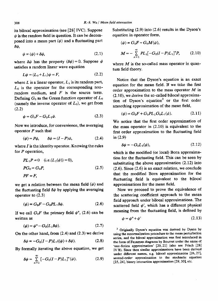
308

its bilocal approximation (see [28] IVC). Suppose 4' is the random field in question. It can be decom- posed into a mean part (4') and a fluctuating part

84,,

4' = (4') + 84, (2.1)

where 84' has the property (84')= 0. Suppose 4' satisfies a random linear wave equation

L4' = (Lo + L1)4' = F, (2.2)

where L is a linear operator, L1 is its random part, Lo is the operator for the corresponding non- random medium, and F is the source term. Defining Go as the Green function operator of Lo (namely the inverse operator of L0), we get from (2.2)

4' = G o F - GoLI4'. (2.3)

Now we introduce, for convenience, the averaging operator P such that

(4') = P4', 64/= (I - P)4', (2.4)

where I is the identity operator. Knowing the rules for P operation,

P L x P = 0 (i.e.(Lx(4')) = 0),

PGo = GoP, (2.5)

P F = F ,

we get a relation between the mean field (4') and the fluctuating field 64' by applying the averaging operator to (2.3)

(4") = G o F - GoPLx84'. (2.6)

If we call G o F the primary field 4'°, (2.6) can be written as

(4") = 4"0_ Go(L~84"). (2.7)

On the other hand, from (2.4) and (2.3) we derive

84" = - ( 7 o ( I - P )Lx ((4") + 84'). (2.8)

By formally iterating the above equation, we get

84"= ~ [ - G o ( I - P ) L 1 ] " ( 4 " ) . (2.9) n = l


Substituting (2.9) into (2.6) results in the Dyson's equation in operator form,

(4') = GoF + GoM(4'),

M = - ~. P L ~ [ - G o ( I - P ) L t ] " P , (2.10) n = l

where M is the so-called mass operator in quan- tum field theory.

Notice that the Dyson's equation is an exact equation for the mean field. If we take the first order approximation to the mass operator M in (2.10), we derive the so-called bilocal approximation of Dyson's equation 2 or the first order smoothing approximation of the mean field,

(4') = GoF + GoPLtGoLI (4 ' ) . (2.11)

We notice that the first order approximation of the mass operator in (2.10) is equivalent to the first order approximation to the fluctuating field in (2.9)

60 = - G o L x ( O ) , (2.12)

which is the modified (or local) Born approximation for the fluctuating field. This can be seen by substituting the above approximation (2.12) into (2.6). Since (2.6) is an exact relation, we conclude that the modified Born approximation for the fluctuating field is equivalent to the bilocal approximations for the mean field.

Now we proceed to prove the equivalence of the scattering coefficient approach to the mean field approach under bilocal approximations. The scattered field 0', which has a different physical meaning from the fluctuating field, is defined by

¢0= 0°+4 ' ' (2.13)

2 Originally Dyson's equation was derived by Dyson by using the renormalization procedure to the mean perturbation series, and the biloeal approximation was first introduced in the form of Feynman diagrams by Bourret under the name of 'one-fiction approximation' [20,21] (also see Frisch [28] IV B). Since then similar approximations have been derived under different names, e.g. bilocal approximation [26, 27], second-order approximation to the stochastic equation [25, 24], binary interaction approximation [29, 30], etc.

R.-$. Wu / Mean field attenuation

where 4/ is the actual random field, 4/° is the primary field, or the field when there are no inhomogeneities. The scattered field 4/' is therefore the field caused by the presence of inhomogeneities.

For a short travel distance, the scattered field 4/' can be calculated by the Born approximation,

4/' = -GoL14/° . (2.14)

Because of the smallness of distance, the mean field (4/) differs only slightly from the primary field 4/°. Therefore, the scattered field 4/' calculated by the Born approximation will be nearly equal to the fluctuating field 84/calculated by the modified Born approximation (2.12). It has been shown that, on average, energy can only flow from the mean field to the random field (in accordance with the second law of thermodynamics, [31]). There- fore, the mean field intensity will decrease con- tinuously due to the energy loss by converting to the random field. If the total energy of the scattered field 4/' is considered to be lost, the field attenuation will have the same rate as the mean field because of the approximate equality between (2.12) and (2.14).

From what has been shown above, we know that the single-scattering approximation and the assumption of total loss of scattered energy lead to the equivalence of the energy scattering coefficient and the mean field attenuation. In fact, unlike the fluctuating field 84/, the energy of the scattered field can be transferred back to the total field. The scattered energy is not necessarily lost totally. Suppose the primary wave is travelling along the x-direction through an n layered medium. For the second layer there is a loss of energy due to single-scattering in the layer but it also gains some energy from the waves scattered by the first layer. For the third layer, the wave will gain scattered energy from single-scattering by the second layer and from double scattering by the first layer. Generally, the n th layer will gain scattered energy from layers 1 through n - 1. In the case of large scale inhomogeneities (ka >> 1), when forward scattering is dominant, the energy

3O9

loss by scattering can be quite different from the result obtained by the Born approximation, especially in the forward direction. Even when the criterion for the Born approximation is satisfied, namely that the fractional energy loss calculated by single-scattering formula is much smaller than 1, the frequency dependence of the total field attenuation obtained by considering multiple scattering will be different from the single scattering approximation. This can be seen from the frequency dependence of the directivity pattern of the scattered energy. The directivity of the mean intensity of the scattered field for the correlation functions e -'/a is [15]

1 f (O) = (1 +4ko2a 2 sin 2 10 2, (2.15) 3)

where O is the angle between incident wave and scattered wave, ko is the wave number and a is the correlation length. For greater k0, more scattered energy will be concentrated in the forward direction so that scattered energy loss will deviate more seriously from the calculation of the single- scattering approximation.

To make the physical meaning clearer, we will use again the one-dimensional wave propagation model over the sliced random slab. Suppose that the primary wave is

4/° = A e ik°x, (2..16)

and there is no energy loss during propagation (neglecting reflections). In spite of this, as shown below, we will find that there is a scattering loss equal to the mean field attenuation, if we follow the scattering coefficient approach.

The one-dimensional scalar wave equation is

(~7 2 + k2)4/= 0,

[~7 2 + ko2(1 + 8s)214/

= [~7 2 + k02(1 + 28s + 8s2)]4/

= 0, (2.17)

where 8s is the fluctuating part of the refractive index (see (1.1)). Neglecting the 8s 2 term and using

310 R.-S. Wu / Mean field attenuation

(2.13), we get

( V 2 + k 2)O ' = - k 2o26Sq~. (2.18)

Now we solve the equation for the scattering field by the first slice. Since a6s is small, we can use the Born approximation

(V 2 + k~)0' = -2k26s00. (2.19)

Knowing the 1-D wave Green function ([34],

g(x , x ' ) - -1 _ikolx-x'l (2.20) -- 2k0 c

and recognizing that

L1 = 2k28s , (2.21)

we obtain the scattered field under the Born approximation

ffJ'(x) = - f g (x , x ')LI~O°(x ') d x '

I = ~ e ik° lx -x ' l (2k~Ss)A e ik°x' d x ' Ago

So ~ i 2 = A ~ o (2ko&) e ik°~ dx

= A eik°Xiko6sa

= d/°iko3sa. (2.22)

In obtaining (2.22) we use the fact that x I> a/> x', where a is the thickness of the layer, in view of the assumption that all the scattered energy goes to the positive x-direction.

For our special model we can, in fact, use a simpler derivation for scattered waves (2.22). We know that the phase deviation for the wave after passing through a layer is koa6s , then the resultant field will be

= A e !k°x+ik°aSs

= 0° + 0'. (2.23)

Therefore, we have

~o'= ¢ , - 0 o

= O°(e ik°ans- 1). (2.24)

When koa6s is small,

~ ' = O°ikoa6s.

The mean intensity of the scattered field is

(1¢'12) = (~, '~0'*)

= (14s°12(k~a28sZ))

= [ O ° l k g a 2 y 2

(2.25)

(2.26)

where y is the r.m.s, deviation of refractive index (see 1.2). If we assume that the total energy scattered by single-scattering is lost, the energy loss by scattering of the whole n-layer slab will be proportional to n(lO'12), because of the indepen- dence between different layers. Therefore the scattering coefficient defined as the fractional energy loss per unit distance by passing through the random slab will be

1 n(14/12)__ n k ~ a 2 y 2

na 14t°[ 2 na

= k ~ a y 2

= 2u, (2.27)

where u is the field randomization coefficient, i.e. the attenuation coefficient of the mean field defined by (1.6) and (1.7). We know that the intensity of the mean field will decrease as

I<¢,)l = = 1¢,°12 e -=~x, (2.28)

so we can see how the premise of the total loss of single-scattered energy leads to an identity between the scattering coefficient and the attenuation coefficient of the mean field energy.

3. On acquiring exper imenta l data of the m e a n

field with an e x a m p l e f rom Lasa

A random medium by mathematical definition is an ensemble or a family of innumerable inhomogeneous components. Each component, with a certain probability of existence, differs from others in its detailed structure, but there are some statistical similarities among all components. When we consider wave propagation in a random

R.-$. Wu / Mean ]ieM attenuation

medium, we are dealing therefore with a random wave, namely an infinitely large family of waves, each propagating in an inhomogeneous medium with a certain probability. The mean of a random wave field is the ensemble average over the whole wave family. Therefore, statistically, the average should be taken over a great many experiments for different members of the considered random medium under the same condition. For seismic wave propagation in the earth, the ensemble average may be approximated by a spatial average in certain cases in view of the ergodicity, or as considered within the framework of a 'pseudo- random medium' [35, 28]. However, when taking spatial averages, the non-random phase relation between waves at different points must be taken into account. In the case of ka >> 1 (i.e. wavelength much smaller than the scale of inhomogeneity), the spatial averaging, which of course should cover an area spanning many correlation lengths, will be taken over many wavelengths. The average of the waves will diminish due to non-random term phase interference, if no phase corrections for waves at different points have been implemented. Therefore, as we take the spatial average, a phase correction, which corresponds to the phase change caused by propagation from the reference point to the point considered with the average velocity, must be performed.

First we consider the 1-D problem. A scalar monochromatic wave A e ik°x is incident on and

propagates in a random medium along the x- direction. Each member of the random medium family is a weakly inhomogeneous medium with a scale of inhomogeneity a (correlation length). We know that the phase deviation of the random wave after passing through a distance a is koaSs, where 8s is the fluctuation of the refractive index; then the wave becomes

~O(a) = A(a) e i(k°a+k°aSs).

When the wave travels within the second layer, since 8s in this layer is uncorrelated with the first layer and is arbitrary, we can consider the two layer medium as being from another member of

311

the random medium family, and so on. Thus for a wave which has traveled a distance na,

~(na) = A(na) exp(ikona

+i ~. koaSs,). (3.1) j=l

For a sufficiently large n, assuming the condition for ergodicity is nearly satisfied, we can take the average of these n waves as the approximation of the ensemble average. However, the phase term e ik°"~, which has nothing to do with the randomness of the medium, will interfere with the result. Therefore we must perform a phase correction e -ik°x to eliminate the phase interference. From the above arguments, we conclude that for one- dimensional problems, the mean field at point x can be approximated by

1j-0 (~0(x)) = x ~O(x') e -ik°x' dx'. (3.2)

Here 4t(x')=A(x')e i*~x') is the measured field at point x' ( ~< x). Therefore

~O(x') e-ik°x' = A(x') e i'*~x'),

where &b(x') is the phase deviation from the field of the homogeneous medium.

If the family of n waves for x = na is taken as a random function or a random process, the ~O(x) is a non-stationary process. The decrease of the mean of the process will approximate the 'attenuation' of the mean field, i.e. the randomization of the field. In the simplified model, in which the phase deviation by passing one layer of thickness a can be with equal probability either A~b~ or --A~ba, where A~a is a fixed small quantity, the total phase deviation then is a Wiener -Levy process with zero mean and a variance equal to

n(Aq~a) 2= (x/a) (Aq~a) 2

([36], Ch. 9). We know from (1.5) that the mean of ~O(x) will decrease exponentially with increasing variance of phase deviation, which explains the decrease of mean field with distance x.

312

The averaging formula for a stationary process

_ 1 fXo+X (0(Xo)) - ~x :xo-~ d/(x') e -ik°x' dx '

would not have any use here. If the process is stationary, its mean should remain unchanged, and the decreasing nature of the mean field can not be obtained.

For three dimensional isotropic problems, in the case of ka >> 1, the measurements on the trans-

verse section (or ones that can be reduced to the transverse section), such as the measurements in a seismic array over many correlation lengths, can be used for the calculation of the mean field. Different ray paths wi th separations larger than

the correlation length can be thought of as different realizations of the random medium. However , no a t tempt has been made, to my knowledge, in obtaining the experimental value of the mean field of seismic waves and comparing them with theoretical calculations. Some authors simply compare those measurements on amplitude at tenuation wi th the theoretical results for the mean field, or equivalently, with scattering

coefficient calculations under the single-scattering approximation. Nevertheless, the coherency measurements using the beam forming method conducted by Mereu and Ojo [37] are closely related to the mean field measurement , though no comparison was made to the mean field formu-

lation. The records of Lasa, Norsa or any large aperture

seismic array can be used to obtain the mean field. Some authors have used these array data in study- ing the statistical propert ies of the under-array media [2, 6, 7]. We will use Aki ' s data on phase fluctuation across Lasa to infer the mean field attenuation. From the ampli tude fluctuation and phase delay fluctuation measurements over the large seismic array, Lasa, consisting of 2 1 × 2 5 vertical seismographs and covering an area of d iameter 200 km, Aki derived a 10 km correlation length for the inhomogeneities, and the velocity fluctuation index

3' = ( ( 8 c / C o ) 2 ) = 4%.

R.-$. Wu / Mean fieM attenuation

From these parameters , we can calculate the randomization coefficient ~,. To compare the calculated values of v with the experiments, we use the phase fluctuation data given by Aki ([2], table 1). In the table he listed the rms (root mean square) phase fluctuations over the seismic m-ray measured in the frequency range 0 . 5 H z - l . 5 H z for 17 events. As we pointed out, when the area of the seismic array is large enough to cover many correlation lengths, the spatial average over the array can approximate the ensemble average. We use only the data for frequencies f rom 0.5 Hz to 1 Hz. Above 1 Hz there are few events to be averaged. The frequencies used and the corresponding average rms phase fluctuations (over all events), as well as the numbers of events over which the

averages were taken, are listed in Table 1.

Table 1

Randomization coefficients in the frequency range 0.5 Hz to 1 Hz for the medium under Lasa

N E (8~) 1/2 i=1 tr~b 2 y2k2a

f(Hz) tr~b N N v~, = 2X0 ~ = 2 (rad.) (10-a/kin) (10-3/km)

0.5 0.57 11 3.2 2.19 0.6 0.52 1 2.7 3.16 0.7 0.59 5 3.5 4.30 0.8 0.74 4 5.5 5.61 1.0 0.94 13 8.8 8.77

(&b~) 1/2 is the rms phase fluctuation for the ith event. N is the number of events over which the average is taken.

For ka >> 1, forward scattering is dominant. If we neglect the amplitude at tenuation in calculat- ing the decrease of the mean field, the randomization coefficient v has a simple relation with the

= . F rom (1.5) rms phase fluctuation tr~b (8~2) 1/2 and (1.6), the ampli tude of the mean field (~) is

obtained as

= 1 0 o l e

= I 'ol e -"x. (3.3)


Therefore, if the average propagation distance X0 in the random medium is known, we can relate the randomization coefficient with the phase variance (8~ 2) as

(&b 2) tr~b 2

u = 2-~0 2X0" (3.4)

On the other hand we can calculate v from the medium parameter 3/and a using

v = "g2k °2------~a (1.7) 2

The v value calculated from the measured o-, (assuming X0 = 50 km) and that from the medium parameters are given in Table 1 and are shown in Fig. 1. The square frequency dependence of v agrees fairly well with the measured phase fluctuations, though the data are not sufficient for a decisive test.

313

when the ensemble mean is taken. It has very little connection with amplitude attenuation. A random wave field is a random complex function of position

¢J(r) = A ( r ) e i*(r)

= A (r) e ~t('~(')>+s'~(')], (4.1)

where $(r) is the random wave, A ( r ) is its amplitude, and ~b(r) is its phase. Both amplitude A and phase ~ are random variables. Also, ($) is the ensemble average of ~b, and 8~b is the fluctuating part. Since phase ~b usually changes much faster than A, we can consider A and $ as linearly independent random variables. Therefore

(~) = (A)(e i*)

= (,4) e i<'t'> e -<8~'2>/2. (4.2)

9 - X

.-.. 7 E ,. 6

X I

3

2

I

i a i , i

0 . 5 0 . 8 I

f ( H z )

Fig. 1. Comparison of ( x ) randomization coefficient t,~ (attenuation coefficient of mean field) calculated from measured phase fluctuations by Aki at Lasa, Montana and (--) v, calculated by

the mean-field formulation from the medium parameters.

4. Ampl i tude attenuation and mean-Reld attenuation

We have shown that the mean-field attenuation is mainly a statistical effect due to phase 'interference' among members of a random wave ensemble

The attenuation of the average amplitude (,4) is usually much slower than the t e r m e -(&/'2)/2, so that the mean-field a t tenua t ion is determined mainly by the phase-interfering term e -<8~2>/2. If we neglect the attenuation of the average amplitude (A), we get

(•) = A0 e-<*'2>/2 ei<,>. (4.3)

This is the result we obtained in (1.6). Therefore the mean-field attenuation derived from the parabolic approximation or other approximation methods is merely accounted for by the statistical effect due to phase randomization, and has nothing to do with the average amplitude attenuation.

From the above analysis, we know that the information concerning amplitude attenuation cannot be extracted or recovered from the mean field formulation.

In order to derive the average amplitude attenuation, we need to remove the phase influence before taking the ensemble average. The best way is to multiply its complex conjugate to the wave field, which corresponds to performing a phase

314

correction for every realization of the ensemble before averaging. Thus we get

(~k~b*) = <A ei6A e -i~') = (A2) . (4.4)

We must solve the equation for the second moment (~b4s*), not for the first moment (~>, in order to describe the average amplitude attenuation of a random wave field.

Recently, Wu [32] has derived the amplitude attenuation from the energy transfer relations within a random slab. The basic idea is the follow- ing. The random slab is sliced into layers of thickness a (correlation length) and the Born approximation is used for each slice to calculate the scattered field. To include the multiple scattering effect, only the energy scattered to the back-halfspace is considered lost (for the case that the wavelength is much smaller than the correlation length), and the energy correction is done for each successive slice.

The derived amplitude attenuation has a quite different behavior from the mean-field attenuation in the high frequency range. Contrary to the mean- field attenuation, which has a unique frequency- dependence regardless of the form of the correlation function of the inhomogeneities, the frequency dependences of the amplitude attenuation have different forms for different correlation functions. For exponential correlation function, the equivalent inverse quality factor of scattering attenuation Qs ~ equals ((22) in [32])

2b 43"2ko3a 3

QsZ = k---~o = 1 + 6k 2a 2 + 8k 4oa 4'


Therefore the apparent amplitude attenuation b, in the high frequency range can be approximated by

2

b ~ 3 ' 4a" (4.7)

In the case of Lasa data, taking 3" = 0.04, a = 10km, vp=6km/sec, we have b-~4×10-S/km for frequencies from 0.5 to 1 Hz. Comparing to Fig. 1, we can see that not only is b much smaller than ~,, but the frequency dependence of b is also quite different from that of v. In addition, from (4.7) the attenuation b is nearly inversely proportional to correlation a when koa is large. This property is expected for attenuation. In the case when the scale of inhomogeneities is larger than the wavelength, a decrease in the size of inhomogeneities will increase the number of scat- terers and therefore increase the scattering energy loss. This is contrary to the mean field attenuation, which decreases with decreasing correlation length a (cf. (1.7) and the related comments).

Fig. 2 shows the comparison between the attenuation measurements and the theoretical prediction by mean field attenuation and by amplitude attenuation. The measurements were made by Aki in Kanto, Japan, using a single-station S-coda-ratio method [3]. In the calculation we took the intrinsic attenuation as 4 x 10 -4, based on the observation that most of the Q-1 curves converge at high frequencies to a certain value, which is assumed to be the intrinsic Q-1 [4]. In general the theoretical curve of amplitude attenuation agrees well with the measurements. The

(4.5) discrepancy between the measured data and the prediction by mean-field attenuation further attest to the inadequacy of the mean field formulation for the problem of amplitude attenuation.

where b is the attenuation coefficient of amplitude due to scattering, ko is the wavenumber for the unperturbed medium, and a is the correlation length. The Qs 1 curve has a peak at koa = 1. In the high frequency range, when koa >> 1,

2

Q s l = 3' (4.6) 2koa"

Acknowledgement

I am grateful to Professor Keiiti Aki for his encouragement, criticism and valuable dis- cussions. He pointed out first to me the incon-

R.-S. Wu / Mean field attenuation 315

10-2

10-3

/ " N(r) = exp ( - r / a )

mean field formulation / / a -~, 0,55 km \ /

3' = 1 2 %

/ / Q~I = 4 x 1 0 -4 / / / /

/ / /

// / 0

/// . f ' f - " - Q " ~ x amplitude attenuation (BHIA)

. . , , I I I

0.1 0.s '1115 ~ ~ 1'2 ~4 .Hzl

Fig. 2. Comparison between measurements of amplitude attenuation and theoretical predictions by the mean field formulation and by the amplitude attenuation formula (4.5).

o is Q-1 of S-wave from measured data at area A, Kanto, Japan;

x is Q- t of S-wave from measured data at area B+C, Kanto, Japan (from Aki, 1980);

- - is O~l = Os 1 + Q~1, calculated Q-1 of S-wave, where Qs ~ is the equivalent O - t of scattering attenuation, and Q~-1

is the intrinsic Q- l , here taken as 4 x 10 -4.

sistency of the mean field concept with actual measurements of seismic waves and has suggested many improvements to this work. This work was done during my stay in the Department of Earth and Planetary Sciences of MIT as a visiting scien- tist sponsored by Professor Aki. I wish to thank the Department and MIT for offering me this opportunity. I have also benefitted from the dis- cussions with Prof. T. Madden, Prof. N. Toks6z, Dr. D. Morgan and Dr. H. Sato. Support for this research was provided in part by Department of Energy contract # DE-AC02-76ER02534.

References

[1] K. Aki, "Analysis of the seismic coda of local earthquakes as scattered waves", Z Geophys. Res. 74, 615-631 (1969).

[2] K. Aki, "Scattering of P waves under the Montana Lasa", Z Geophys. Res. 78, 1334-1346 (1973).

[3] K. Aki, "Attenuation of shear waves in the lithosphere for frequencies from 0.05 to 25 Hz", Phys. Earth Planet. Int. 21, 50-60 (1980).

[4] K. Aki, "Scattering and attenuation of shear waves in the lithosphere", J. Geophys. Res. 85, 6496-6504 (1980).

[5] S.A. Fedotov and S.A. Boldyrev, "Frequency dependence of the body-wave absorption in the crust and the upper mantle of the Kuril-Island chain", Izv. Earth Physics 9, 17-33 (1969).

[6] J. Capon, "Characterization of crust and upper mantle structure under Lasa as a random medium", Bull. Seis. Soc. Amer. 64, 235-266 (1974).

[7] K.A. Berteussen, A. Christoffersson, E.S. Husebye, and A. Dahle, "Wave scattering theory in analysis of P wave anomalies at NORSAR and LASA", Geophys. J. Roy. Astr. Soc. 42, 403-417 (1975).

[8] K. Aki and B. Chouet, "Origin of coda waves: source, attenuation and scattering effects", Jr. Geophys. Res. 80, 3322-3342 (1975).

[9] B. Chouet, Source, Scattering and attenuation effects on high frequency seismic waves, Ph.D. Thesis, Massachusetts Institute of Technology, Cambridge, MA (1976).

[10] M. Tsujiura, "Spectral analysis of the coda waves from local earthquakes", Bull. Earthquake Res. Inst. Tokyo Univ. 53, 1-48 (1978).

[11] T.G. Rautian and V.I. Khalturin, "The use of coda for determination of the earthquake source spectrum", Bull. Seis. Soc. Amer. 68, 923-948 (1978).

[12] S.W. Roecker, Seismicity and tectonics of the Pamir- Hindu Kush Region of Central Asia, Ph.D. Thesis, Massachusetts Institute of Technology, Cambridge, MA, Ch. 5 (1981).

[13] H. Sato, "Energy propagation including scattering effects, single isotropic scattering approximation", J. Phy. Earth 25, 27-41 (1977).

[14] C.L. Pekeris, "Note on the scattering of radiation in an inhomogeneous medium", Phys. Rev. 71, 268-269 (1947).

[15] L.A. Chernov, Wave Propagation in a Random Medium, McGraw-Hill, New York (1960).

[16] P.R. Beaudet, "Elastic wave propagation in heterogeneous media", Bull. Seismol. Soc. Amer. 60, 769-784 (1970).

[17] V.K. Varadan, V.V. Varadan, and Y.H. Pao, "Multiple scattering of elastic waves by cylinders of arbitrary cross section. I. SH waves", Z Acoust. Soc. Amer. 63 (5), 1310-1319 (1978).

[18] V.K. Varadan and V.V. Varadan, "Frequency dependence of elastic (SH-) wave velocity and attenuation in anisotropic two phase media", Wave Motion 1, 53-63 (1979).

[19] H. Sato, "Wave propagation in one-dimensional inhomogeneous elastic media", J. Phys. Earth 27, 455- 466 (1979).

[20] R.C. Bourret, "Seismic waves in a randomly stratified earth model", preprint (1980).

316 R.-S. Wu / Mean field attenuation

[21] R.C. Bourret, "Stochastically perturbated fields, with application to wave propagation in random media", Nuovo Cimento 26, 1-31 (1962).

[22] R.C. Bourret, "Propagation of randomly perturbated fields", Canad. Z Phys. 40, 782-790 (1-962).

[23] J.B. Keller, "Wave propagation in random media", Proc. Syrup. AppL Math. 13, 227-246 (1962).

[24] J.B. Keller, "Stochastic equations and wave propagation in random media", Proc. Syrup. Appl. Math. 16, 145-170 (1964).

[25] F.C. Karal and J.B. Keller, "Elastic, electromagnetic and other waves in a random medium", Z Math. Phys. 5 (4), 537-549 (1964).

[26] V.I. Tartaski and M.E. Gertsenshtein, "Propagation of waves in a medium with strong fluctuation of the refractive index", Soviet Physics JETP 17 (2), 458-463 (1963).

[27] V.I. Tatarski, "Propagation of electromagnetic waves in a medium with strong dielectric-constant fluctuations", Soviet Physics JETP 19 (4) 946-953 (1964).

[28] V. Frisch, Wave Propagation in Random Media, Prob- abilistic Methods in Applied Mathematics, Vol. 1, Academic Press, New York (1968) 76-198.

[29] M.S. Howe, "Wave propagation in random media", J. Fluid Mech. 45, 769-783 (1971).

[30] M.S. Howe, "On wave scattering by random inhomogeneities with application to the theory of weak bores", J. Fluid Mech. 45, 785-804 (1971).

[31] M.S. Howe, "Conservation of energy in random media, with application to the theory of sound absorption by an inhomogeneous flexible plate", Proc. Roy. Soc. London A 331, 479-496 (1973).

[32] R.S. Wu, "Attenuation of short period seismic waves due to scattering", Geophys. Res. Len. 9 (1), 9-12 (1982).

[33] B.J. Usinski, The Elements of Wave Propagation in Random Media, McGraw-Hill, New York (1977).

[34] P.M. Morse and H. Feshbach, Methods of Theoretical Physics, McGraw-Hill, New York (1953).

[35] J. Bass, Les Fonctions Pseudo-Aleatoires, Gauthier- Villars (1962).

[36] A. Papoulis, Probability, Random Variables and Stochas- tic Process, McGraw-Hill, New York (1965).

[37] R.F. Mereu, and S. Ojo, "Seismic wave propagation through a crust with random lateral and vertical inhomogeneities", A G U 1980 Spring Meeting, Abstract 593 (1980).

mean field attenuation and amplitude ai~fenuation due …wrs/publication/journal/journal1981... ·...

Documents