matrix iterative methods from the historical, analytic ...strakos/download/2016_munich.pdf ·...
TRANSCRIPT

Matrix iterative methods from the historical, analytic, application,and computational perspective
Zdenek Strakos(Charles University and Academy of Sciences of the Czech Republic, Prague )
IDGK Compact Course, TU Munich, November 2016
1 / 109
Meaning of the words
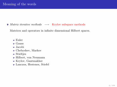
Matrix iterative methods −→ Krylov subspace methods
Matrices and operators in infinite dimensional Hilbert spaces.
EulerGaussJacobiChebyshev, MarkovStieltjesHilbert, von NeumannKrylov, GantmakherLanczos, Hestenes, Stiefel
2 / 109
Meaning of the words
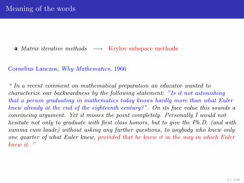
Matrix iterative methods −→ Krylov subspace methods
Cornelius Lanczos, Why Mathematics, 1966
“ In a recent comment on mathematical preparation an educator wanted tocharacterize our backwardness by the following statement: ”Is it not astonishingthat a person graduating in mathematics today knows hardly more than what Eulerknew already at the end of the eighteenth century?”. On its face value this sounds aconvincing argument. Yet it misses the point completely. Personally I would nothesitate not only to graduate with first class honors, but to give the Ph.D. (and withsumma cum laude) without asking any further questions, to anybody who knew onlyone quarter of what Euler knew, provided that he knew it in the way in which Eulerknew it. ”
3 / 109
Meaning of the words
Matrix iterative methods −→ Krylov subspace methods
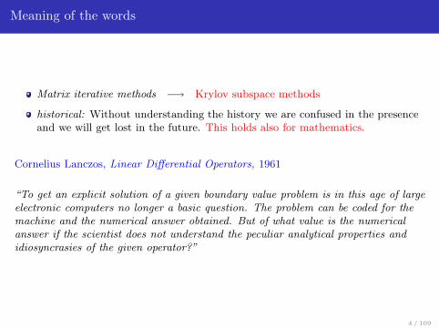
historical: Without understanding the history we are confused in the presenceand we will get lost in the future. This holds also for mathematics.
Cornelius Lanczos, Linear Differential Operators, 1961
“To get an explicit solution of a given boundary value problem is in this age of largeelectronic computers no longer a basic question. The problem can be coded for themachine and the numerical answer obtained. But of what value is the numericalanswer if the scientist does not understand the peculiar analytical properties andidiosyncrasies of the given operator?”
4 / 109
Meaning of the words
Matrix iterative methods −→ Krylov subspace methods
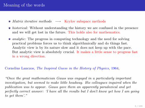
historical: Without understanding the history we are confused in the presenceand we will get lost in the future. This holds also for mathematics.
analytic: The progress in computing technology and the need for solvingpractical problems forces us to think algorithmically and do things fast.Analytic view is by its nature slow and it does not keep up with the pace.But analytic view is absolutely crucial. It makes a little sense to progress fastin a wrong direction.
Cornelius Lanczos, The Inspired Guess in the History of Physics, 1964,
“Once the great mathematician Gauss was engaged in a particularly importantinvestigation, but seemed to make little headway. His colleagues inquired when thepublication was to appear. Gauss gave them an apparently paradoxical and yetperfectly correct answer: ‘I have all the results but I don’t know yet how I am goingto get them’.”
5 / 109
Meaning of the words
Matrix iterative methods −→ Krylov subspace methods
historical: Without understanding the history we are confused in the presenceand we will get lost in the future. This holds also for mathematics.
analytic: The progress in computing technology and the need for solvingpractical problems forces us to think algorithmically and do things fast.Analytic view is by its nature slow and it does not keep up with the pace.But analytic view is absolutely crucial. It makes a little sense to progress fastin a wrong direction.
application: Development and application of mathematics lives in anunbreakable symbiosis. I do not believe in “pure” against “applied”mathematics. This division is artificial, caused by proudness and ambitions. Asa malign disease it leads mathematics to fragmentation and the fields ofmathematics to dangerous isolation. Applications are like a fresh water. Anyapplication must honor the assumptions of the theory.
6 / 109

Meaning of the words - application
Henri Poincare, 1909, graduate of the Polytechnique
“The scientist does not study nature because it is useful; he studies it because hedelights in it, and he delights in it because it is beautiful. If nature were notbeautiful, it would not be worth knowing, and if nature were not worth knowing, lifewould not be worth living. ...I mean that deeper beauty coming from the harmonious order of the parts, and thata pure intelligence can grasp.
Science has had marvelous applications, but a science that would only haveapplications in mind would not be science anymore, it would be only cookery.”
7 / 109
Meaning of the words
Matrix iterative methods −→ Krylov subspace methods
historical: Without understanding the history we are confused in the presenceand we will get lost in the future. This holds also for mathematics.
analytic: The progress in computing technology and the need for solvingpractical problems forces us to think algorithmically and do things fast.Analytic view is by its nature slow and it does not keep up with the pace.But analytic view is absolutely crucial. It makes a little sense to progress fastin a wrong direction.
application: Development and application of mathematics lives in anunbreakable symbiosis. I do not believe in “pure” against “applied”mathematics. This division is artificial, caused by proudness and ambitions. Asa malign disease it leads mathematics to fragmentation and the fields ofmathematics to dangerous isolation. Applications are like a fresh water. Anyapplication must honor the assumptions of the theory.
computational: Computing is a very involved process. Computers should servein solving properly mathematically formulated problems. Mathematics mustrespect limitations of the computing technology.
8 / 109
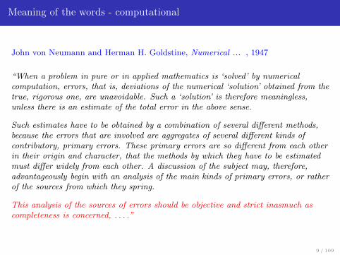
Meaning of the words - computational
John von Neumann and Herman H. Goldstine, Numerical ... , 1947
“When a problem in pure or in applied mathematics is ‘solved’ by numericalcomputation, errors, that is, deviations of the numerical ‘solution’ obtained from thetrue, rigorous one, are unavoidable. Such a ‘solution’ is therefore meaningless,unless there is an estimate of the total error in the above sense.
Such estimates have to be obtained by a combination of several different methods,because the errors that are involved are aggregates of several different kinds ofcontributory, primary errors. These primary errors are so different from each otherin their origin and character, that the methods by which they have to be estimatedmust differ widely from each other. A discussion of the subject may, therefore,advantageously begin with an analysis of the main kinds of primary errors, or ratherof the sources from which they spring.
This analysis of the sources of errors should be objective and strict inasmuch ascompleteness is concerned, . . . .”
9 / 109

Cornelius Lanczos, March 9, 1947
On (what are now called) the Lanczos and CG methods:
“The reason why I am strongly drawn to suchapproximation mathematics problems is ... the fact thata very “economical” solution is possible only when it is very “adequate”.
To obtain a solution in very few stepsmeans nearly always that one has found a waythat does justice to the inner nature of the problem.”
10 / 109

Albert Einstein, March 18, 1947
“Your remark on the importance ofadapted approximation methods makes verygood sense to me, and I am convincedthat this is a fruitful mathematical aspect,and not just a utilitarian one.”
11 / 109

Albert Einstein, March 18, 1947
“Your remark on the importance ofadapted approximation methods makes verygood sense to me, and I am convincedthat this is a fruitful mathematical aspect,and not just a utilitarian one.”
Main principle behind Krylov subspace methods:
Highly nonlinear adaptation of the iterations to the problem.
11 / 109
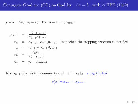
Conjugate Gradient (CG) method for Ax = b with A HPD (1952)
r0 = b − Ax0, p0 = r0 . For n = 1, . . . , nmax :
αn−1 =r∗n−1rn−1
p∗n−1Apn−1
xn = xn−1 + αn−1pn−1 , stop when the stopping criterion is satisfied
rn = rn−1 − αn−1Apn−1
βn =r∗nrn
r∗n−1rn−1
pn = rn + βnpn−1
Here αn−1 ensures the minimization of ‖x − xn‖A along the line
z(α) = xn−1 + αpn−1 .
12 / 109
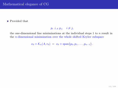
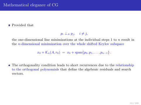
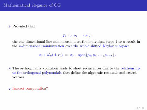
Mathematical elegance of CG
Provided that
pi ⊥A pj , i 6= j,
the one-dimensional line minimizations at the individual steps 1 to n result inthe n-dimensional minimization over the whole shifted Krylov subspace
x0 + Kn(A, r0) = x0 + spanp0, p1, . . . , pn−1 .
13 / 109
Mathematical elegance of CG
Provided that
pi ⊥A pj , i 6= j,
the one-dimensional line minimizations at the individual steps 1 to n result inthe n-dimensional minimization over the whole shifted Krylov subspace
x0 + Kn(A, r0) = x0 + spanp0, p1, . . . , pn−1 .
The orthogonality condition leads to short recurrences due to the relationshipto the orthogonal polynomials that define the algebraic residuals and searchvectors.
Inexact computation?
13 / 109

Antoine de Saint-Exupery , The Wisdom of the Sands, 1944
“I would not bid you pore upon a heap of stones, and turn them over and over, inthe vain hope of learning from them the secret of meditation. For on the level of thestones there is no question of meditation; for that, the temple must have come intobeing. But, once it is built, a new emotion sways my heart, and when I go away, Iponder on the relations between the stones. ...
I must begin by feeling love; and I must first observe a wholeness. After that Imay proceed to study the components and their groupings. But I shall not trouble toinvestigate these raw materials unless they are dominated by something on which myheart is set. Thus I began by observing the triangle as a whole; then I sought tolearn in it the functions of its component lines. ...
So, to begin with, I practise contemplation. After that, if I am able, I analyseand explain. ...
Little matter the actual things that are linked together; it is the links that I mustbegin by apprehending and interpreting.”
14 / 109
Outline
1 What are the Krylov subspace methods and what kind of mathematics isinvolved?
2 Linear projections onto highly nonlinear Krylov subspaces
3 Model reduction and moment matching
4 Convergence and spectral information
5 Inexact computations and numerical stability
6 Functional analysis and infinite dimensional considerations
7 Operator preconditioning, discretization and algebraic computation
8 HPC computations with Krylov subspace methods?
9 Myths about Krylov subspace methods
15 / 109
1. What are the Krylov subspace methods and whatkind of mathematics is involved?
16 / 109

1 Historical development and context
Mechanical quadrature
Newton, Cotes 1720s
Gauss quadrature
Gauss 1814
Gauss quadrature and
orthogonal polynomials
Jacobi 1826
Generalisations of the
Gauss quadrature,
minimal partial realisation
Christoffel 1858/77
Three-term recurrences
and continued fractions
Brouncker, Wallis 1650s
Infinite series expansions
and continued fractions
Euler 1744/48
Continued fractions and
three-term recurrence for
orthogonal polynomials
Chebyshev 1855/59
Continued fractions and
Chebyshev inequalities
Chebyshev 1855,
Markov, Stieltjes 1884
Real symmetric matrices
have real eigenvalues,
interlacing property
Cauchy 1824
Reduction of bilinear
form to tridiagonal form
Jacobi 1848
Diagonalisation of
quadratic forms
Jacobi 1857
Jordan canonical form
Weierstrass 1868,
Jordan 1870
Minimal polynomial
Frobenius 1878
Analytic theory of continued fractions,
Riemann-Stieltjes integral,
solution of the moment problem
Stieltjes 1894
Jacobi form (or matrix)
Hellinger & Toeplitz 1914
Foundations of functional analysis, including continuous spectrum, resolution
of unity, self-adjoined operators, Hilbert space
Hilbert 1906-1912
Orthogonalisation via
the Gramian
Gram 1883
Orthogonalisation algorithms
for functions and vectors
Schmidt 1905/07, Szász 1910
Mathematical foundations of
quantum mechanics
Hilbert 1926/27,
von Neumann 1927/32,
Wintner 1929
Representation theorem
Riesz 1909
Modern numerical analysis
von Neumann & Goldstine 1947
Turing 1948
Krylov subspace methods
Lanczos 1950/52, Hestenes & Stiefel 1952
Transformation of the
characteristic equation
Krylov 1931
Orthogonalisation idea
Laplace 1820
1950
1650
Secular equation of the
moon
Lagrange 1774
Characteristic equation
Cauchy 1840
Krylov sequences
Gantmacher 1934
17 / 109

2 Lanczos, Hestenes and Stiefel
Numerical analysis
Rounding error analysis
Least squares solutions
Gaussian elimination
Matrix theory
Optimisation
Structure and sparsity
Convex geometry
Convergence analysis
Cornelius Lanczos
An iteration method for the solution
of the eigenvalue problem of linear
diff ti l d i t l t 1950
Polynomial preconditioningIterative methods Stopping criteria
Vandermonde determinant
Floating point computationsCost of computations
Data uncertainty
y
Projections
OrthogonalisationOrthogonal polynomials
Linear algebraApproximation theory
Chebyshev, Jacobi and
Legendre polynomials
Minimising functionals
g ydifferential and integral operators, 1950
Solution of systems of linear equations
by minimized iterations, 1952
Chebyshev polynomials in the solution
of large-scale linear systems, 1952
Cauchy-Schwarz inequality
General inner products
Gauss-Christoffel quadrature Riemann-Stieltjes integral
Sturm sequences
Rayleigh quotients Differential and integral operators
Fredholm problem
Functional analysis
g p y
Continued fractions
Liouville-Neumann expansion
Magnus R. Hestenes & Eduard Stiefel
Methods of conjugate gradients for
solving linear systems, 1952
Green s function
Fourier series
Dirichlet and Fejér kernel
Trigonometric interpolation
Gibbs oscillation
Gauss Christoffel quadrature Riemann Stieltjes integral
Real analysis
Dirichlet and Fejér kernel
18 / 109
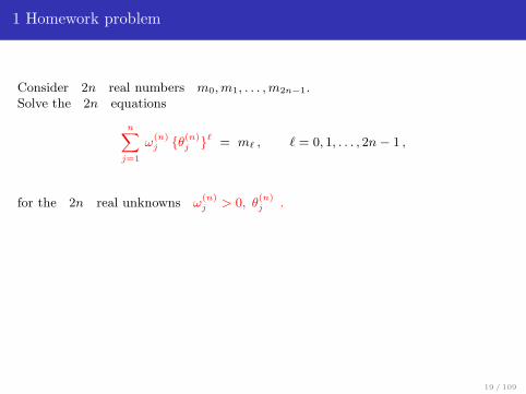
1 Homework problem
Consider 2n real numbers m0, m1, . . . , m2n−1.Solve the 2n equations
n∑
j=1
ω(n)j θ(n)
j ℓ = mℓ , ℓ = 0, 1, . . . , 2n − 1 ,
for the 2n real unknowns ω(n)j > 0, θ
(n)j .
19 / 109
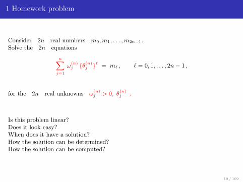
1 Homework problem
Consider 2n real numbers m0, m1, . . . , m2n−1.Solve the 2n equations
n∑
j=1
ω(n)j θ(n)
j ℓ = mℓ , ℓ = 0, 1, . . . , 2n − 1 ,
for the 2n real unknowns ω(n)j > 0, θ
(n)j .
Is this problem linear?Does it look easy?When does it have a solution?How the solution can be determined?How the solution can be computed?
19 / 109
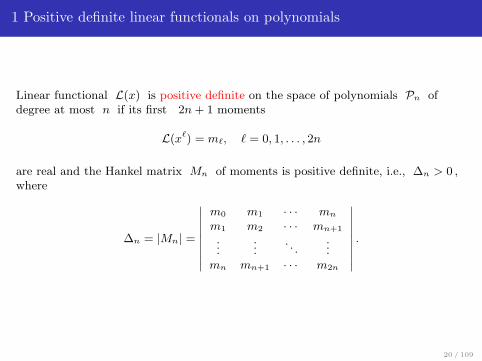
1 Positive definite linear functionals on polynomials
Linear functional L(x) is positive definite on the space of polynomials Pn ofdegree at most n if its first 2n + 1 moments
L(xℓ) = mℓ, ℓ = 0, 1, . . . , 2n
are real and the Hankel matrix Mn of moments is positive definite, i.e., ∆n > 0 ,where
∆n = |Mn| =
∣∣∣∣∣∣∣∣∣
m0 m1 · · · mn
m1 m2 · · · mn+1
......
. . ....
mn mn+1 · · · m2n
∣∣∣∣∣∣∣∣∣
.
20 / 109
1 Stieltjes moment problem (1894) of order n
With the positive definite L(x) we can restrict ourselves to real polynomials of areal variable and write, using a non-decreasing positive distribution function µdefined on the real axis having finite limits at ±∞,
L(f) =
∫f(x) dµ(x) ,
with the inner product
(p, q) := L(p(x)q(x)) =
∫p(x)q(x) dµ(x) .
21 / 109
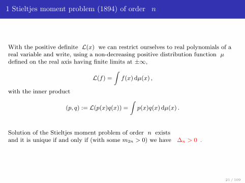
1 Stieltjes moment problem (1894) of order n
With the positive definite L(x) we can restrict ourselves to real polynomials of areal variable and write, using a non-decreasing positive distribution function µdefined on the real axis having finite limits at ±∞,
L(f) =
∫f(x) dµ(x) ,
with the inner product
(p, q) := L(p(x)q(x)) =
∫p(x)q(x) dµ(x) .
Solution of the Stieltjes moment problem of order n existsand it is unique if and only if (with some m2n > 0) we have ∆n > 0 .
21 / 109
1 The unknown ω(n)j , θ
(n)j ?
Cholesky decomposition of the matrix of moments Mn = LnLTn
The entries of the ℓth row of the the inverse L−1n give the coefficients of the
ℓth orthonormal polynomial determined by the positive definite linearfunctional L(x) associated with the matrix of moments Mn .
Roots of the ℓth orthogonal polynomial give the quadrature nodes θ(ℓ)j . The
weights ω(ℓ)j are given by the formula for the interpolatory quadrature.
Computations are done differently
(Gragg and Harrod, Gautschi, Laurie, ...)
O’Leary, S, Tichy, On Sensitivity of Gauss-Christoffel quadrature, NumerischeMathematik, 107, 2007, pp. 147 –174
Pranic, Pozza, S, Gauss quadrature for quasi-definite linear functionals, IMA J.Numer. Anal, 2016 (to appear)
22 / 109
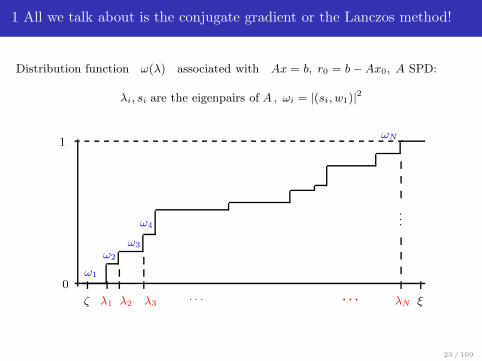
1 All we talk about is the conjugate gradient or the Lanczos method!
Distribution function ω(λ) associated with Ax = b, r0 = b − Ax0, A SPD:
λi, si are the eigenpairs of A , ωi = |(si, w1)|2
...
0
1
ω1
ω2
ω3
ω4
ωN
ζ λ1 λ2 λ3. . . . . . λN ξ
23 / 109

1 Spectral decomposition A =∑N
ℓ=1 λℓ sℓs∗
ℓ
Symbolically
w∗1Aw1 = w∗
1
(N∑
ℓ=1
λℓ sℓs∗ℓ
)w1 ≡ w∗
1
(∫ b
a
λdE(λ)
)w1
=
N∑
ℓ=1
λℓ w∗1sℓ s∗ℓw1 =
N∑
ℓ=1
λℓ ωℓ =
∫ b
a
λ dω(λ) ,
where dE(λℓ) ≡ sℓs∗ℓ and
I =N∑
ℓ=1
sℓs∗ℓ ≡
∫ b
a
dE(λ) .
Hilbert (1906, 1912, 1928), Von Neumann (1927, 1932), Wintner (1929) .
24 / 109
2. Linear projections onto highly nonlinear Krylovsubspaces
References:
J. Liesen. and Z.S., Krylov Subspace Methods, Principles and Analysis. OxfordUniversity Press (2013), Chapter 2
25 / 109
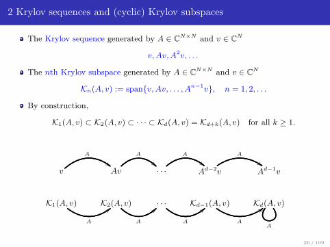
2 Krylov sequences and (cyclic) Krylov subspaces
The Krylov sequence generated by A ∈ CN×N and v ∈ C
N
v, Av, A2v, . . .
The nth Krylov subspace generated by A ∈ CN×N and v ∈ C
N
Kn(A, v) := spanv, Av, . . . , An−1v, n = 1, 2, . . .
By construction,
K1(A, v) ⊂ K2(A, v) ⊂ · · · ⊂ Kd(A, v) = Kd+k(A, v) for all k ≥ 1.
v
A
##Av
A
· · ·
A
""Ad−2v
A
$$Ad−1v
K1(A, v)
A
;;K2(A, v)
A
>>· · ·
A
<<Kd−1(A, v)
A
::Kd(A, v)
A
DD
26 / 109
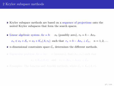
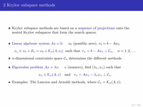
2 Krylov subspace methods
Krylov subspace methods are based on a sequence of projections onto thenested Krylov subspaces that form the search spaces.
Linear algebraic system Ax = b: x0 (possibly zero), r0 = b − Ax0.
xn ∈ x0 + Sn = x0 + Kn(A, r0) such that rn = b − Axn ⊥ Cn, n = 1, 2, . . .
n-dimensional constraints space Cn determines the different methods.
Eigenvalue problem Ax = λx: v (nonzero), find (λn, xn) such that
xn ∈ Kn(A, v) and rn = Axn − λnxn ⊥ Cn.
Examples: The Lanczos and Arnoldi methods, where Cn = Kn(A, v).
27 / 109
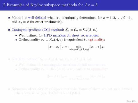
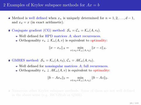
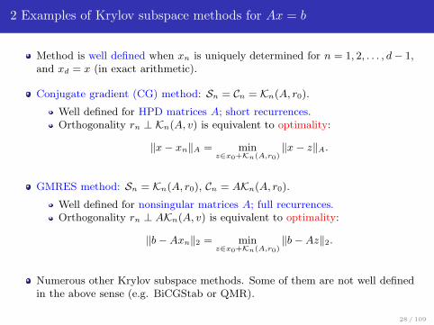
2 Examples of Krylov subspace methods for Ax = b
Method is well defined when xn is uniquely determined for n = 1, 2, . . . , d − 1,and xd = x (in exact arithmetic).
Conjugate gradient (CG) method: Sn = Cn = Kn(A, r0).
Well defined for HPD matrices A; short recurrences.Orthogonality rn ⊥ Kn(A, v) is equivalent to optimality:
‖x − xn‖A = minz∈x0+Kn(A,r0)
‖x − z‖A.
GMRES method: Sn = Kn(A, r0), Cn = AKn(A, r0).
Well defined for nonsingular matrices A; full recurrences.Orthogonality rn ⊥ AKn(A, v) is equivalent to optimality:
‖b − Axn‖2 = minz∈x0+Kn(A,r0)
‖b − Az‖2.
Numerous other Krylov subspace methods. Some of them are not well definedin the above sense (e.g. BiCGStab or QMR).
28 / 109
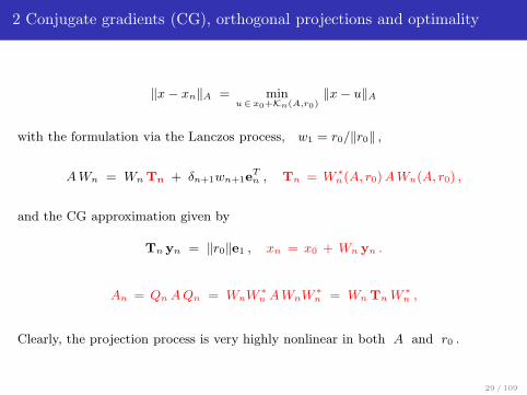
2 Conjugate gradients (CG), orthogonal projections and optimality
‖x − xn‖A = minu∈ x0+Kn(A,r0)
‖x − u‖A
with the formulation via the Lanczos process, w1 = r0/‖r0‖ ,
A Wn = Wn Tn + δn+1wn+1eTn , Tn = W ∗
n(A, r0) AWn(A, r0) ,
and the CG approximation given by
Tn yn = ‖r0‖e1 , xn = x0 + Wn yn .
An = Qn A Qn = WnW ∗n AWnW ∗
n = Wn Tn W ∗n ,
Clearly, the projection process is very highly nonlinear in both A and r0 .
29 / 109
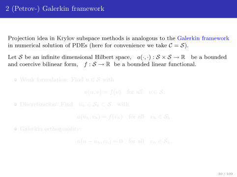
2 (Petrov-) Galerkin framework
Projection idea in Krylov subspace methods is analogous to the Galerkin frameworkin numerical solution of PDEs (here for convenience we take C = S).
Let S be an infinite dimensional Hilbert space, a(·, ·) : S × S → R be a boundedand coercive bilinear form, f : S → R be a bounded linear functional.
Weak formulation: Find u ∈ S with
a(u, v) = f(v) for all v ∈ S .
Discretization: Find uh ∈ Sh ⊂ S with
a(uh, vh) = f(vh) for all vh ∈ Sh.
Galerkin orthogonality:
a(u − uh, vh) = 0 for all vh ∈ Sh.
30 / 109
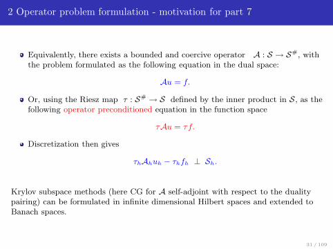
2 Operator problem formulation - motivation for part 7
Equivalently, there exists a bounded and coercive operator A : S → S#, withthe problem formulated as the following equation in the dual space:
Au = f.
Or, using the Riesz map τ : S# → S defined by the inner product in S , as thefollowing operator preconditioned equation in the function space
τAu = τf.
Discretization then gives
τhAhuh − τhfh ⊥ Sh.
Krylov subspace methods (here CG for A self-adjoint with respect to the dualitypairing) can be formulated in infinite dimensional Hilbert spaces and extended toBanach spaces.
31 / 109
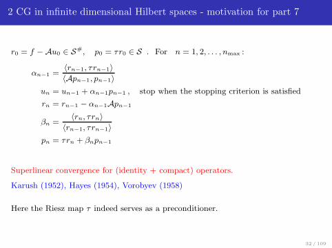
2 CG in infinite dimensional Hilbert spaces - motivation for part 7
r0 = f −Au0 ∈ S#, p0 = τr0 ∈ S . For n = 1, 2, . . . , nmax :
αn−1 =〈rn−1, τrn−1〉〈Apn−1, pn−1〉
un = un−1 + αn−1pn−1 , stop when the stopping criterion is satisfied
rn = rn−1 − αn−1Apn−1
βn =〈rn, τrn〉
〈rn−1, τrn−1〉pn = τrn + βnpn−1
Superlinear convergence for (identity + compact) operators.
Karush (1952), Hayes (1954), Vorobyev (1958)
Here the Riesz map τ indeed serves as a preconditioner.
32 / 109

2 Summary and motivation
Krylov subspace methods for solving linear algebraic problems are based onlinear projections onto nested subspaces.
Krylov subspaces and therefore the resulting methods are highly nonlinear inthe data defining the problem.
The nonlinearity allows to adapt to the problem as the iteration proceeds.This is not apparent, e.g., from the derivation of CG based on theminimization of the quadratic functional, and this fact has affected negativelythe presentation of Krylov subspace methods in textbooks.
The adaptation can be better understood via the model reduction and momentmatching properties of Krylov subspace methods.
33 / 109
3. Model reduction and moment matching
References:
J. Liesen. and Z.S., Krylov Subspace Methods, Principles and Analysis. OxfordUniversity Press (2013), Chapter 3
34 / 109
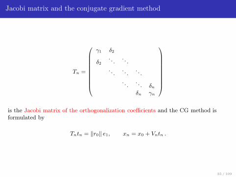
Jacobi matrix and the conjugate gradient method
Tn =
γ1 δ2
δ2
. . .. . .
. . .. . .
. . .
. . .. . . δn
δn γn
is the Jacobi matrix of the orthogonalization coefficients and the CG method isformulated by
Tntn = ‖r0‖ e1, xn = x0 + Vntn .
35 / 109

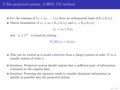
3 The projected system, A HPD, CG method
Let the columns of Vn = [v1, . . . , vn] form an orthonormal basis of Kn(A, r0).
Matrix formulation of xn ∈ x0 + Kn(A, r0) and rn ⊥ Kn(A, r0):
xn = x0 + Vntn
and tn ∈ Cn is found by solving
V ∗n AVn tn = ‖r0‖e1.
This can be viewed as a model reduction from a (large) system of order N to a(small) system of order n.
Intuition: Projected system should capture fast a sufficient part of informationcontained in the original data.
Intuition: Powering the operator tends to transfer dominant information asquickly as possible into the projected system.
36 / 109
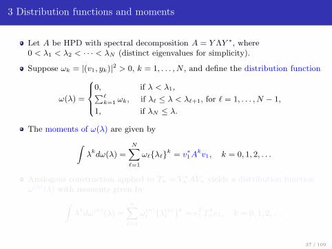
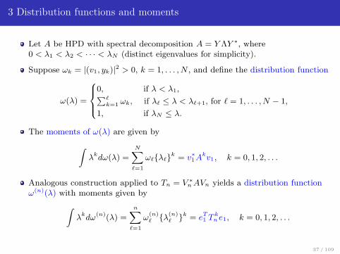
3 Distribution functions and moments
Let A be HPD with spectral decomposition A = Y ΛY ∗, where0 < λ1 < λ2 < · · · < λN (distinct eigenvalues for simplicity).
Suppose ωk = |(v1, yk)|2 > 0, k = 1, . . . , N , and define the distribution function
ω(λ) =
0, if λ < λ1,∑ℓ
k=1 ωk, if λℓ ≤ λ < λℓ+1, for ℓ = 1, . . . , N − 1,
1, if λN ≤ λ.
The moments of ω(λ) are given by
∫λkdω(λ) =
N∑
ℓ=1
ωℓλℓk = v∗1Akv1, k = 0, 1, 2, . . .
Analogous construction applied to Tn = V ∗n AVn yields a distribution function
ω(n)(λ) with moments given by
∫λkdω(n)(λ) =
n∑
ℓ=1
ω(n)ℓ λ(n)
ℓ k = eT1 T k
ne1, k = 0, 1, 2, . . .
37 / 109

3 Stieltjes recurrence and Jacobi matrix
Let φ0(λ) ≡ 1, φ1(λ), . . . , φn(λ) be the first n + 1 orthonormal
polynomials corresponding to the distribution function ω(λ) .
Then, writing Φn(λ) = [φ0(λ), . . . , φn−1(λ)]∗ ,
λ Φn(λ) = Tn Φn(λ) + δn+1 φn(λ) en
represents the Stieltjes recurrence (1893-4), see Chebyshev (1855), Brouncker(1655), Wallis (1656), Toeplitz and Hellinger (1914) with the Jacobi matrix
Tn ≡
γ1 δ2
δ2 γ2
. . .
. . .. . .
δn
δn γn
, δl > 0 , ℓ = 2, . . . , n .
38 / 109
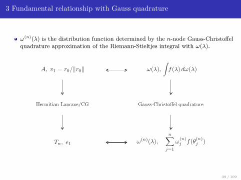
3 Fundamental relationship with Gauss quadrature
ω(n)(λ) is the distribution function determined by the n-node Gauss-Christoffelquadrature approximation of the Riemann-Stieltjes integral with ω(λ).
39 / 109
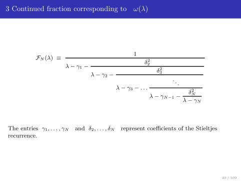
3 Continued fraction corresponding to ω(λ)
FN (λ) ≡ 1
λ − γ1 − δ22
λ − γ2 − δ23
λ − γ3 − . . .
. . .
λ − γN−1 − δ2N
λ − γN
The entries γ1, . . . , γN and δ2, . . . , δN represent coefficients of the Stieltjesrecurrence.
40 / 109
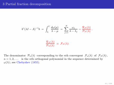
3 Partial fraction decomposition
b∗(λI − A)−1b =
∫ U
L
dω(µ)
λ − µ=
N∑
j=1
ωj
λ − λj
=RN (λ)
PN (λ),
RN (λ)
PN(λ)≡ FN (λ)
The denominator Pn(λ) corresponding to the nth convergent Fn(λ) of FN (λ) ,n = 1, 2, . . . is the nth orthogonal polynomial in the sequence determined byω(λ) ; see Chebyshev (1855).
41 / 109
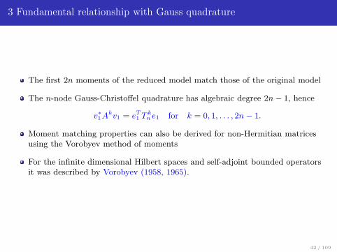
3 Fundamental relationship with Gauss quadrature
The first 2n moments of the reduced model match those of the original model
The n-node Gauss-Christoffel quadrature has algebraic degree 2n − 1, hence
v∗1Akv1 = eT
1 T kne1 for k = 0, 1, . . . , 2n − 1.
Moment matching properties can also be derived for non-Hermitian matricesusing the Vorobyev method of moments
For the infinite dimensional Hilbert spaces and self-adjoint bounded operatorsit was described by Vorobyev (1958, 1965).
42 / 109
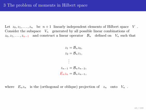
3 The problem of moments in Hilbert space
Let z0, z1, . . . , zn be n + 1 linearly independent elements of Hilbert space V .Consider the subspace Vn generated by all possible linear combinations ofz0, z1, . . . , zn−1 and construct a linear operator Bn defined on Vn such that
z1 = Bnz0,
z2 = Bnz1,
...
zn−1 = Bnzn−2,
Enzn = Bnzn−1,
where Enzn is the (orthogonal or oblique) projection of zn onto Vn .
43 / 109
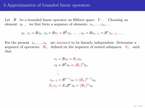
3 Approximation of bounded linear operators
Let B be a bounded linear operator on Hilbert space V . Choosing anelement z0 , we first form a sequence of elements z1, . . . , zn, . . .
z0, z1 = Bz0, z2 = Bz1 = B2z0, . . . , zn = Bzn−1 = Bnzn−1, . . .
For the present z1, . . . , zn are assumed to be linearly independent. Determine asequence of operators Bn defined on the sequence of nested subspaces Vn suchthat
z1 = Bz0 = Bnz0,
z2 = B2z0 = (Bn)2z0,
...
zn−1 = Bn−1z0 = (Bn)n−1z0,
Enzn = EnBnz0 = (Bn)nz0.
44 / 109
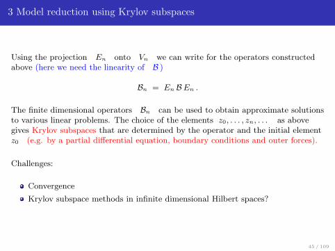
3 Model reduction using Krylov subspaces
Using the projection En onto Vn we can write for the operators constructedabove (here we need the linearity of B )
Bn = En B En .
The finite dimensional operators Bn can be used to obtain approximate solutionsto various linear problems. The choice of the elements z0, . . . , zn, . . . as abovegives Krylov subspaces that are determined by the operator and the initial elementz0 (e.g. by a partial differential equation, boundary conditions and outer forces).
Challenges:
Convergence
Krylov subspace methods in infinite dimensional Hilbert spaces?
45 / 109

4. Convergence and spectral information
References
J. Liesen. and Z.S., Krylov Subspace Methods, Principles and Analysis. OxfordUniversity Press (2013), Chapter 5, Sections 5.1 - 5.7
T. Gergelits and Z.S., Composite convergence bounds based on Chebyshevpolynomials and finite precision conjugate gradient computations, Numer. Alg.65, 759-782 (2014)
46 / 109
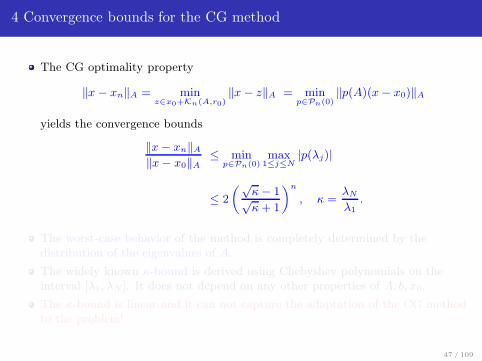
4 Convergence bounds for the CG method
The CG optimality property
‖x − xn‖A = minz∈x0+Kn(A,r0)
‖x − z‖A = minp∈Pn(0)
‖p(A)(x− x0)‖A
yields the convergence bounds
‖x − xn‖A
‖x − x0‖A
≤ minp∈Pn(0)
max1≤j≤N
|p(λj)|
≤ 2
(√κ − 1√κ + 1
)n
, κ =λN
λ1.
The worst-case behavior of the method is completely determined by thedistribution of the eigenvalues of A.
The widely known κ-bound is derived using Chebyshev polynomials on theinterval [λ1, λN ]. It does not depend on any other properties of A, b, x0.
The κ-bound is linear and it can not capture the adaptation of the CG methodto the problem!
47 / 109
4 CG, large outliers and condition numbers
Consider the desired accuracy ǫ , κs(A) ≡ λN−s/λ1 . Then
k = s +
⌈ln(2/ǫ)
2
√κs(A)
⌉
CG steps will produce the approximate solution xn satisfying
‖x − xn‖A ≤ ǫ ‖x − x0‖A .
This statement qualitatively explains superlinear convergence ofCG at the presence of large outliers in the spectrum, assumingexact arithmetic.
48 / 109
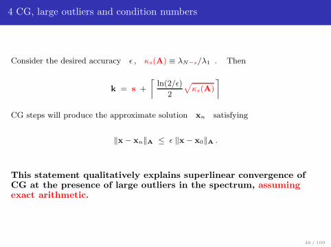
4 Adaptive Chebyshev bound?
0 20 40 60 80 100
10−15
10−10
10−5
100
49 / 109
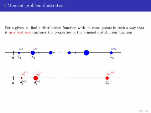
4 Moment problem illustration
For a given n find a distribution function with n mass points in such a way thatit in a best way captures the properties of the original distribution function
0
tω1
λ1
②ω2
λ2
r . . . r ⑤ ωN
λN
0
sω
(n)1
θ(n)1
③ω
(n)2
θ(n)2
. . . ω
(n)n
θ(n)n
50 / 109

4 CG and Gauss quadrature errors
At any iteration step n , CG represents the matrix formulation of the n-pointGauss quadrature of the R-S integral determined by A and r0 ,
∫f(λ) dω(λ) =
n∑
i=1
ω(n)i f(θ
(n)i ) + Rn(f) .
For f(λ) ≡ λ−1 the formula takes the form
‖x − x0‖2A
‖r0‖2= n-th Gauss quadrature +
‖x − xn‖2A
‖r0‖2.
This has became a base for the CG error estimation (see above); see the surveys inS and Tichy, 2002; Meurant and S, 2006; Liesen and S, 2013.
51 / 109
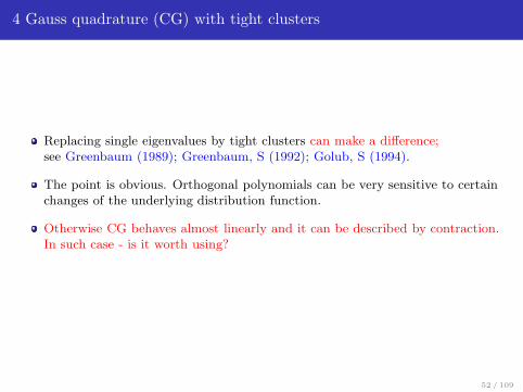
4 Gauss quadrature (CG) with tight clusters
Replacing single eigenvalues by tight clusters can make a difference;see Greenbaum (1989); Greenbaum, S (1992); Golub, S (1994).
The point is obvious. Orthogonal polynomials can be very sensitive to certainchanges of the underlying distribution function.
Otherwise CG behaves almost linearly and it can be described by contraction.In such case - is it worth using?
52 / 109
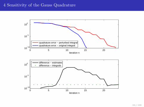
4 Sensitivity of the Gauss Quadrature
0 5 10 15 2010
−10
10−5
100
iteration n
quadrature error − perturbed integralquadrature error − original integral
0 5 10 15 2010
−10
10−5
100
iteration n
difference − estimatesdifference − integrals
53 / 109
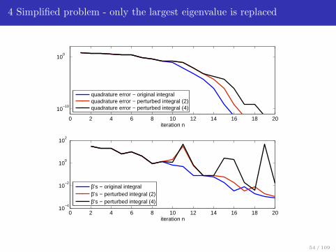
4 Simplified problem - only the largest eigenvalue is replaced
0 2 4 6 8 10 12 14 16 18 20
10−10
100
iteration n
quadrature error − original integralquadrature error − perturbed integral (2)quadrature error − perturbed integral (4)
0 2 4 6 8 10 12 14 16 18 2010
−4
10−2
100
102
iteration n
β’s − original integralβ’s − perturbed integral (2)β’s − perturbed integral (4)
54 / 109
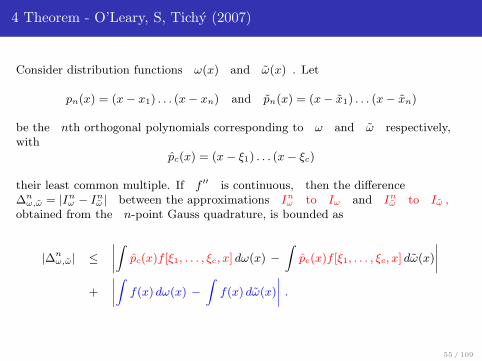
4 Theorem - O’Leary, S, Tichy (2007)
Consider distribution functions ω(x) and ω(x) . Let
pn(x) = (x − x1) . . . (x − xn) and pn(x) = (x − x1) . . . (x − xn)
be the nth orthogonal polynomials corresponding to ω and ω respectively,with
pc(x) = (x − ξ1) . . . (x − ξc)
their least common multiple. If f ′′ is continuous, then the difference∆n
ω,ω = |Inω − In
ω | between the approximations Inω to Iω and In
ω to Iω ,obtained from the n-point Gauss quadrature, is bounded as
|∆nω,ω| ≤
∣∣∣∣∫
pc(x)f [ξ1, . . . , ξc, x] dω(x) −∫
pc(x)f [ξ1, . . . , ξc, x] dω(x)
∣∣∣∣
+
∣∣∣∣∫
f(x) dω(x) −∫
f(x) dω(x)
∣∣∣∣ .
55 / 109
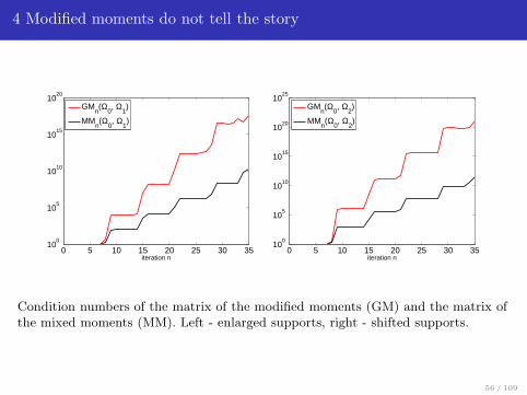
4 Modified moments do not tell the story
0 5 10 15 20 25 30 3510
0
105
1010
1015
1020
iteration n
GMn(Ω
0, Ω
1)
MMn(Ω
0, Ω
1)
0 5 10 15 20 25 30 3510
0
105
1010
1015
1020
1025
iteration n
GMn(Ω
0, Ω
2)
MMn(Ω
0, Ω
2)
Condition numbers of the matrix of the modified moments (GM) and the matrix ofthe mixed moments (MM). Left - enlarged supports, right - shifted supports.
56 / 109
4 Summary of the CG/Lanczos part
1 Gauss-Christoffel quadrature for a small number of quadrature nodes can behighly sensitive to small changes in the distribution function enlarging itssupport.
2 In particular, the difference between the corresponding quadratureapproximations (using the same number of quadrature nodes) can be manyorders of magnitude larger than the difference between the integrals beingapproximated.
3 This sensitivity in Gauss-Christoffel quadrature can be observedfor discontinuous, continuous, and even analytic distribution functions,and for analytic integrands uncorrelated with changes in the distributionfunctions and with no singularity close to the interval of integration.
57 / 109
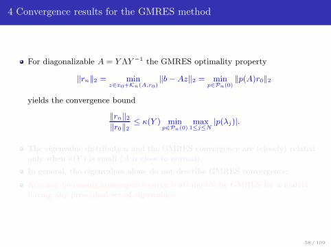
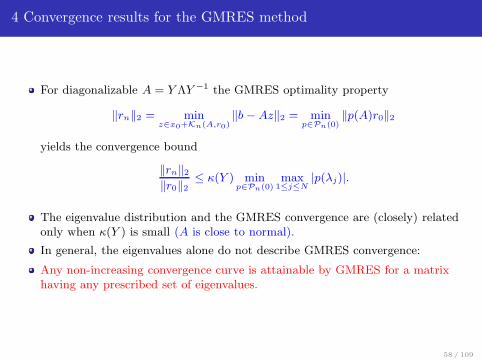
4 Convergence results for the GMRES method
For diagonalizable A = Y ΛY −1 the GMRES optimality property
‖rn‖2 = minz∈x0+Kn(A,r0)
‖b − Az‖2 = minp∈Pn(0)
‖p(A)r0‖2
yields the convergence bound
‖rn‖2
‖r0‖2≤ κ(Y ) min
p∈Pn(0)max
1≤j≤N|p(λj)|.
The eigenvalue distribution and the GMRES convergence are (closely) relatedonly when κ(Y ) is small (A is close to normal).
In general, the eigenvalues alone do not describe GMRES convergence:
Any non-increasing convergence curve is attainable by GMRES for a matrixhaving any prescribed set of eigenvalues.
58 / 109

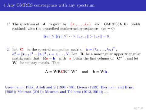
4 Any GMRES convergence with any spectrum
Given any spectrum and any sequence of the nonincreasing residual norms, acomplete parametrization is known of the set of all GMRES associated matricesand right hand sides.
The set of problems for which the distribution of eigenvalues alone does notcorrespond to convergence behavior is not of measure zero and it is not pathological.
Widespread eigenvalues alone can not be identified with poor convergence.
Clustered eigenvalues alone can not be identified with fast convergence.
Equivalent orthogonal matrices; pseudospectrum indication.
59 / 109
4 Any GMRES convergence with any spectrum
1 The spectrum of A is given by λ1, . . . , λN and GMRES(A,b) yieldsresiduals with the prescribed nonincreasing sequence (x0 = 0)
‖r0‖ ≥ ‖r1‖ ≥ · · · ≥ ‖rN−1‖ > ‖rN‖ = 0 .
2 Let C be the spectral companion matrix, h = (h1, . . . , hN )T ,h2
i = ‖ri−1‖2 − ‖ri‖2 , i = 1, . . . , N . Let R be a nonsingular upper triangularmatrix such that Rs = h with s being the first column of C−1 , and letW be unitary matrix. Then
A = WRCR−1
W∗ and b = Wh .
Greenbaum, Ptak, Arioli and S (1994 - 98); Liesen (1999); Eiermann and Ernst(2001); Meurant (2012); Meurant and Tebbens (2012, 2014); .....
60 / 109
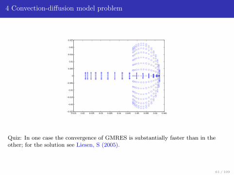
4 Convection-diffusion model problem
0.015 0.02 0.025 0.03 0.035 0.04 0.045 0.05 0.055 0.06 0.065−0.025
−0.02
−0.015
−0.01
−0.005
0
0.005
0.01
0.015
0.02
0.025
Quiz: In one case the convergence of GMRES is substantially faster than in theother; for the solution see Liesen, S (2005).
61 / 109
5. Inexact computation and numerical stability
References
J. Liesen. and Z.S., Krylov Subspace Methods, Principles and Analysis. OxfordUniversity Press (2013), Chapter 5, Sections 5.8 - 5.11
T. Gergelits and Z.S., Composite convergence bounds based on Chebyshevpolynomials and finite precision conjugate gradient computations, Numer. Alg.65, 759-782 (2014)
62 / 109
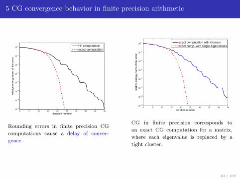
5 CG convergence behavior in finite precision arithmetic
0 5 10 15 20 25 30 35 40 4510
−14
10−12
10−10
10−8
10−6
10−4
10−2
100
iteration number
rela
tive
ener
gy n
orm
of t
he e
rror
FP computationexact computation
Rounding errors in finite precision CG
computations cause a delay of conver-
gence.
0 5 10 15 20 25 30 35 40 4510
−14
10−12
10−10
10−8
10−6
10−4
10−2
100
iteration number
rela
tive
ener
gy n
orm
of t
he e
rror
exact computation with clustersexact comp. with single eigenvalues
CG in finite precision corresponds to
an exact CG computation for a matrix,
where each eigenvalue is replaced by a
tight cluster.
63 / 109
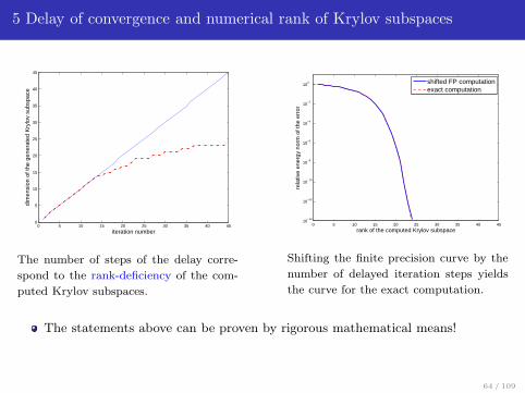
5 Delay of convergence and numerical rank of Krylov subspaces
0 5 10 15 20 25 30 35 40 450
5
10
15
20
25
30
35
40
45
iteration number
dim
ensi
on o
f the
gen
erat
ed K
rylo
v su
bspa
ce
The number of steps of the delay corre-
spond to the rank-deficiency of the com-
puted Krylov subspaces.
0 5 10 15 20 25 30 35 40 4510
−14
10−12
10−10
10−8
10−6
10−4
10−2
100
rank of the computed Krylov subspace
rela
tive
ener
gy n
orm
of t
he e
rror
shifted FP computationexact computation
Shifting the finite precision curve by the
number of delayed iteration steps yields
the curve for the exact computation.
The statements above can be proven by rigorous mathematical means!
64 / 109
5 Mathematical model of FP CG
CG in finite precision arithmetic can be seen as the exact arithmetic CG for theproblem with the slightly modified distribution function with larger support, i.e.,with single eigenvalues replaced by tight clusters.
Paige (1971-80), Greenbaum (1989),Parlett (1990), S (1991), Greenbaum and S (1992), Notay (1993), ... , Druskin,Kniznermann, Zemke, Wulling, Meurant, ...Recent reviews and updates in Meurant and S, Acta Numerica (2006); Meurant(2006); Liesen and S (2013).
One particular consequence is becoming very relevant: In FP computations, thecomposite convergence bounds eliminating large outlying eigenvalues at the cost ofone iteration per eigenvalue (see Axelsson (1976), Jennings (1977)) are not valid.
65 / 109
5 Optimality in finite precision Lanczos (CG) computations?
In exact arithmetic, local orthogonality properties of CG are equivalent to theglobal orthogonality properties and therefore also to the CG optimality recalledabove.
In finite precision arithmetic the local orthogonality properties are preservedproportionally to machine precision, but the global orthogonality and thereforethe optimality wrt the underlying distribution function is lost.
in finite precision arithmetic computations (or, more generally, in inexactKrylov subspace methods) the optimality property does not have any easilyformulated meaning with respect to the subspaces generated by the computedresidual (or direction) vectors.
Using the results of Greenbaum from 1989, it does have, however, a welldefined meaning with respect to the particular distribution functions definedby the original data and the rounding errors in the steps 1 trough n.
66 / 109
5 Optimality in finite precision Lanczos (CG) computations?
Consider the following mathematically equivalent formulation of CG
A Wn = Wn Tn + δn+1wn+1eTn , Tn = W ∗
n(A, r0) AWn(A, r0) ,
and the CG approximation given by
Tn yn = ‖r0‖e1 , xn = x0 + Wn yn .
Greenbaum proved that the Jacobi matrix computed in finite precisionarithmetic can be considered a left principal submatrix of a certain largerJacobi matrix having all its eigenvalues close to the eigenvalues of the originalmatrix A.
This is equivalent to saying that convergence behavior in the first n steps ofthe given finite precision Lanczos computation can equivalently be described asthe result of the exact Gauss quadrature for certain distribution function thatdepends on n having tight clusters of points of increase around the originaleigenvalues of A.
67 / 109

5 Analysis of the FP CG behaviour
68 / 109

5 Numerical stability of GMRES
In finite precision, the loss of orthogonality using the modified Gram-SchmidtGMRES is inversely proportional to the normwise relative backward error
‖b − Axn‖2
‖b‖2 + ‖A‖2‖xn‖2.
Loss of orthogonality (blue) and normwise relative backward error (red) for aconvection-diffusion model problem with two different “winds”:
0 5 10 15 20 25 30 35 40 4510
−18
10−16
10−14
10−12
10−10
10−8
10−6
10−4
10−2
100
0 10 20 30 40 50 6010
−18
10−16
10−14
10−12
10−10
10−8
10−6
10−4
10−2
100
It can be shown that the MGS-GMRES is normwise backward stable.
69 / 109

5 Delay of convergence due to inexactness
0 20 40 60 80 100
10−15
10−10
10−5
100
?
0 100 200 300 400 500 600 700 800
10−15
10−10
10−5
100
iteration number
residualsmooth uboundbackward errorloss of orthogonalityapproximate solutionerror
Here numerical inexactness due to roundoff. How much may we relax accuracy ofthe most costly operations without causing an unwanted delay and/or affecting themaximal attainable accuracy? That will be crucial in exascale computations.
70 / 109
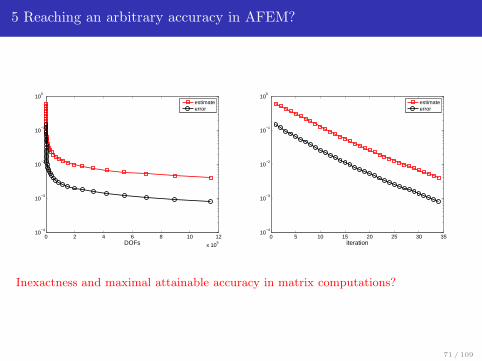
5 Reaching an arbitrary accuracy in AFEM?
0 2 4 6 8 10 12
x 105
10−4
10−3
10−2
10−1
100
DOFs
estimateerror
0 5 10 15 20 25 30 3510
−4
10−3
10−2
10−1
100
iteration
estimateerror
Inexactness and maximal attainable accuracy in matrix computations?
71 / 109
6. Functional analysis and infinite dimensionalconsiderations
References
J. Malek and Z.S., Preconditioning and the Conjugate Gradient Method in theContext of Solving PDEs. SIAM Spotlight Series, SIAM (2015), Chapter 9
72 / 109
6 Bounded invertible operators
Let V be an infinite dimensional Hilbert space, B a bounded linear operator onV that has a bounded inversion. Consider the problem
B u = f , f ∈ V .
The identity operator on an infinite dimensional Hilbert space is not compact.
Since BB−1 = I , it follows that B can not be compact.
Approximation of B by finite dimensional operatorsBn : V → Vn , Vn is finite dimensional?
73 / 109

6 Compact and finite dimensional operators
A uniform (in norm) limit of finite dimensional operators Bn is a compactoperator.
Every compact operator on a Hilbert space is a uniform limit of a sequence offinite dimensional operators.
A uniform limit of compact operators is a compact operator.
Bounded invertible operators in Hilbert (holds also for Banach) spaces can not beapproximated in norm to an arbitrary accuracy by neither compact nor finitedimensional operators! Approximation can be considered only in the sense of strongconvergence (pointwise limit); for the method of moments see Vorobyev (1958, 1965)
‖Bn w − Bw‖ → 0 ∀w ∈ V .
74 / 109
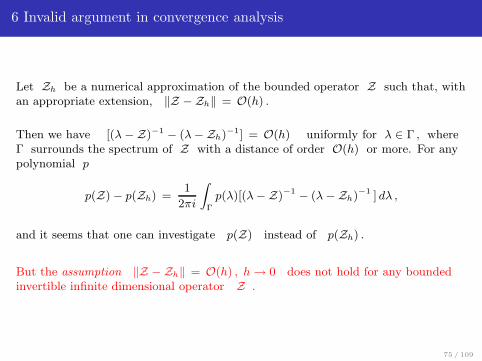
6 Invalid argument in convergence analysis
Let Zh be a numerical approximation of the bounded operator Z such that, withan appropriate extension, ‖Z − Zh‖ = O(h) .
Then we have [(λ −Z)−1 − (λ −Zh)−1] = O(h) uniformly for λ ∈ Γ , whereΓ surrounds the spectrum of Z with a distance of order O(h) or more. For anypolynomial p
p(Z) − p(Zh) =1
2πi
∫
Γ
p(λ)[(λ −Z)−1 − (λ −Zh)−1 ] dλ ,
and it seems that one can investigate p(Z) instead of p(Zh) .
But the assumption ‖Z − Zh‖ = O(h) , h → 0 does not hold for any boundedinvertible infinite dimensional operator Z .
75 / 109
7. Operator preconditioning, discretization andalgebraic computation
References
J. Malek and Z.S., Preconditioning and the Conjugate Gradient Method in theContext of Solving PDEs. SIAM Spotlight Series, SIAM (2015)
J. Papez, J.Liesen and Z.S., Distribution of the discretization and algebraicerror in numerical solution of partial differential equations, Linear Alg. Appl.449, 89-114 (2014)
J. Papez, Z.S., and M. Vohralık Estimating and localizing the algebraic and totalnumerical errors using flux reconstructions, (2016, submitted for publication)
J. Papez and Z.S., Subtleties of the residual-based a posteriori error estimatorfor total error, (2016, submitted for publication)
76 / 109
Functional analysis and iterative methods
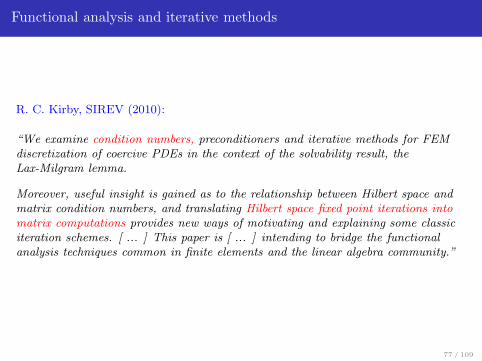
R. C. Kirby, SIREV (2010):
“We examine condition numbers, preconditioners and iterative methods for FEMdiscretization of coercive PDEs in the context of the solvability result, theLax-Milgram lemma.
Moreover, useful insight is gained as to the relationship between Hilbert space andmatrix condition numbers, and translating Hilbert space fixed point iterations intomatrix computations provides new ways of motivating and explaining some classiciteration schemes. [ ... ] This paper is [ ... ] intending to bridge the functionalanalysis techniques common in finite elements and the linear algebra community.”
77 / 109

Functional analysis and iterative methods
K. A. Mardal and R. Winther, NLAA (2011):
“The main focus will be on an abstract approach to the construction ofpreconditioners for symmetric linear systems in a Hilbert space setting [ ... ] Thediscussion of preconditioned Krylov space methods for the continuous systems will bea starting point for a corresponding discrete theory.
By using this characterization it can be established that the conjugate gradientmethod converges [ ... ] with a rate which can be bounded by the condition number [... ] However, if the operator has a few eigenvalues far away from the rest of thespectrum, then the estimate is not sharp. In fact, a few ‘bad eigenvalues’ will havealmost no effect on the asymptotic convergence of the method.”
78 / 109
Functional analysis and iterative methods
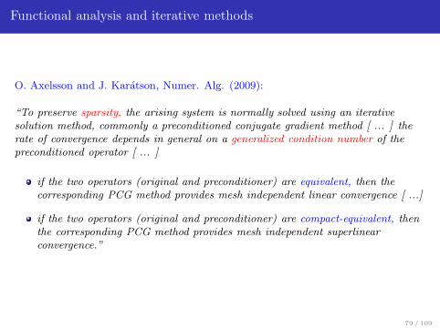
O. Axelsson and J. Karatson, Numer. Alg. (2009):
“To preserve sparsity, the arising system is normally solved using an iterativesolution method, commonly a preconditioned conjugate gradient method [ ... ] therate of convergence depends in general on a generalized condition number of thepreconditioned operator [ ... ]
if the two operators (original and preconditioner) are equivalent, then thecorresponding PCG method provides mesh independent linear convergence [ ...]
if the two operators (original and preconditioner) are compact-equivalent, thenthe corresponding PCG method provides mesh independent superlinearconvergence.”
79 / 109
7 Mesh independent condition number
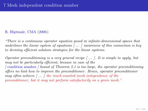
R. Hiptmair, CMA (2006):
“There is a continuous operator equation posed in infinite-dimensional spaces thatunderlines the linear system of equations [ ... ] awareness of this connection is keyto devising efficient solution strategies for the linear systems.
Operator preconditioning is a very general recipe [ ... ]. It is simple to apply, butmay not be particularly efficient, because in case of the[ condition number ] bound of Theorem 2.1 is too large, the operator preconditioningoffers no hint how to improve the preconditioner. Hence, operator preconditionermay often achieve [ ... ] the much-vaunted mesh independence of thepreconditioner, but it may not perform satisfactorily on a given mesh.”
80 / 109

7 Linear asymptotic behavior?
V. Faber, T. Manteuffel and S. V. Parter, Adv. in Appl. Math. (1990):
“For a fixed h, using a preconditioning strategy based on an equivalent operator maynot be superior to classical methods [ ... ] Equivalence alone is not sufficient for agood preconditioning strategy. One must also choose an equivalent operator forwhich the bound is small.
There is no flaw in the analysis, only a flaw in the conclusions drawn from theanalysis [ ... ] asymptotic estimates ignore the constant multiplier. Methods withsimilar asymptotic work estimates may behave quite differently in practice.”
81 / 109
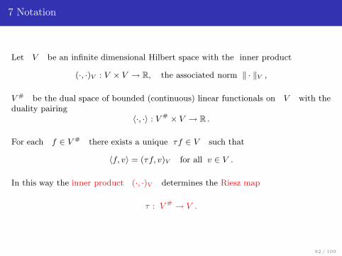
7 Notation
Let V be an infinite dimensional Hilbert space with the inner product
(·, ·)V : V × V → R, the associated norm ‖ · ‖V ,
V # be the dual space of bounded (continuous) linear functionals on V with theduality pairing
〈·, ·〉 : V # × V → R .
For each f ∈ V # there exists a unique τf ∈ V such that
〈f, v〉 = (τf, v)V for all v ∈ V .
In this way the inner product (·, ·)V determines the Riesz map
τ : V # → V .
82 / 109
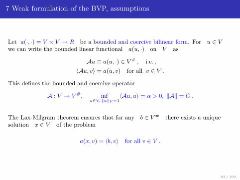
7 Weak formulation of the BVP, assumptions
Let a(·, ·) = V × V → R be a bounded and coercive bilinear form. For u ∈ Vwe can write the bounded linear functional a(u, ·) on V as
Au ≡ a(u, ·) ∈ V # , i.e. ,
〈Au, v〉 = a(u, v) for all v ∈ V .
This defines the bounded and coercive operator
A : V → V #, infu∈V, ‖u‖V =1
〈Au, u〉 = α > 0, ‖A‖ = C .
The Lax-Milgram theorem ensures that for any b ∈ V # there exists a uniquesolution x ∈ V of the problem
a(x, v) = 〈b, v〉 for all v ∈ V .
83 / 109

7 Operator problem formulation
Equivalently,〈Ax − b, v〉 = 0 for all v ∈ V ,
which can be written as the equation in V # ,
Ax = b , A : V → V #, x ∈ V, b ∈ V # .
We will consider A self-adjoint with respect to the duality pairing 〈·, ·〉 .
84 / 109
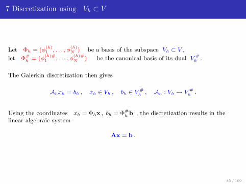
7 Discretization using Vh ⊂ V
Let Φh = (φ(h)1 , . . . , φ
(h)N ) be a basis of the subspace Vh ⊂ V ,
let Φ#h = (φ
(h)#1 , . . . , φ
(h)#N ) be the canonical basis of its dual V #
h .
The Galerkin discretization then gives
Ahxh = bh , xh ∈ Vh , bh ∈ V #h , Ah : Vh → V #
h .
Using the coordinates xh = Φhx , bh = Φ#h b , the discretization results in the
linear algebraic system
Ax = b .
85 / 109
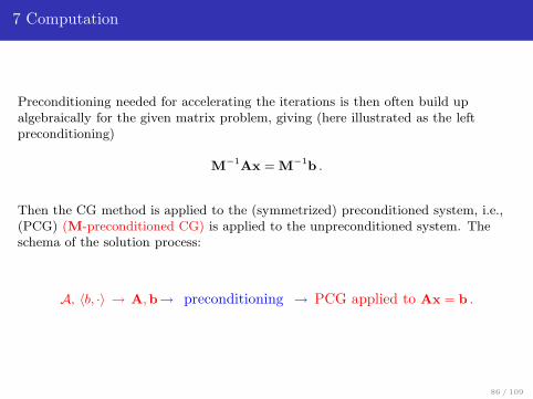
7 Computation
Preconditioning needed for accelerating the iterations is then often build upalgebraically for the given matrix problem, giving (here illustrated as the leftpreconditioning)
M−1
Ax = M−1
b .
Then the CG method is applied to the (symmetrized) preconditioned system, i.e.,(PCG) (M-preconditioned CG) is applied to the unpreconditioned system. Theschema of the solution process:
A, 〈b, ·〉 → A,b→ preconditioning → PCG applied to Ax = b .
86 / 109
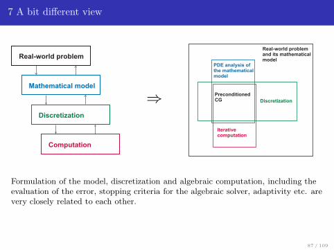
7 A bit different view
⇒
Formulation of the model, discretization and algebraic computation, including theevaluation of the error, stopping criteria for the algebraic solver, adaptivity etc. arevery closely related to each other.
87 / 109
7 Operator formulation of the problem
Recall that the inner product (·, ·)V defines the Riesz map τ .It can be used to transform the equation in V #
Ax = b , A : V → V #, x ∈ V, b ∈ V # .
into the equation in V
τAx = τb, τA : V → V, x ∈ V, τb ∈ V ,
This transformation is called operator preconditioning.
88 / 109
7 The mathematically best preconditioning?
With the choice of the inner product (·, ·)V = a(·, ·) we get
a(u, v) = 〈Au, v〉 = a(τAu, v)
i.e.,τ = A−1 , and the preconditioned system x = A−1b .
The inner product can be defined using an operator
B ≈ A , (·, ·)V = (·, ·)B = 〈Bu, v〉 .
Thenτ = B−1 , and the preconditioned system B−1Ax = B−1b .
What does it mean B ≈ A ?
Concept of norm equivalence and spectral equivalence of operators.
89 / 109
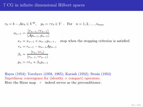
7 CG in infinite dimensional Hilbert spaces
r0 = b −Ax0 ∈ V #, p0 = τr0 ∈ V . For n = 1, 2, . . . , nmax
αn−1 =〈rn−1, τrn−1〉〈Apn−1, pn−1〉
xn = xn−1 + αn−1pn−1 , stop when the stopping criterion is satisfied
rn = rn−1 − αn−1Apn−1
βn =〈rn, τrn〉
〈rn−1, τrn−1〉pn = τrn + βnpn−1
Hayes (1954); Vorobyev (1958, 1965); Karush (1952); Stesin (1954)Superlinear convergence for (identity + compact) operators.Here the Riesz map τ indeed serves as the preconditioner.
90 / 109
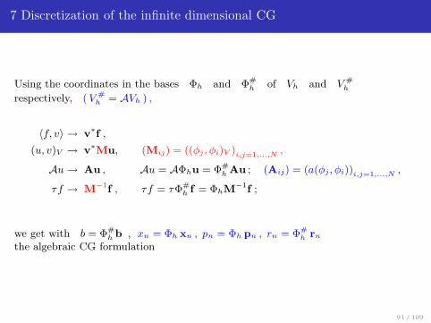
7 Discretization of the infinite dimensional CG
Using the coordinates in the bases Φh and Φ#h of Vh and V #
h
respectively, ( V #h = AVh ) ,
〈f, v〉 → v∗f ,
(u, v)V → v∗Mu, (Mij) = ((φj , φi)V )
i,j=1,...,N,
Au → Au , Au = AΦhu = Φ#h Au ; (Aij) = (a(φj , φi))i,j=1,...,N
,
τf → M−1
f , τf = τΦ#h f = ΦhM
−1f ;
we get with b = Φ#h b , xn = Φh xn , pn = Φh pn , rn = Φ#
h rn
the algebraic CG formulation
91 / 109
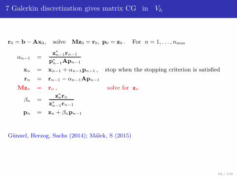
7 Galerkin discretization gives matrix CG in Vh
r0 = b − Ax0, solve Mz0 = r0, p0 = z0 . For n = 1, . . . , nmax
αn−1 =z∗
n−1rn−1
p∗n−1Apn−1
xn = xn−1 + αn−1pn−1 , stop when the stopping criterion is satisfied
rn = rn−1 − αn−1Apn−1
Mzn = rn , solve for zn
βn =z∗
nrn
z∗n−1rn−1
pn = zn + βnpn−1
Gunnel, Herzog, Sachs (2014); Malek, S (2015)
92 / 109
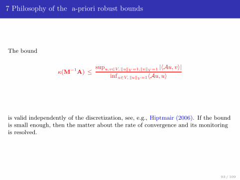
7 Philosophy of the a-priori robust bounds
The bound
κ(M−1A) ≤
supu,v∈V, ‖u‖V =1,‖v‖V =1 |〈Au, v〉|infu∈V, ‖u‖V =1〈Au, u〉
is valid independently of the discretization, see, e.g., Hiptmair (2006). If the boundis small enough, then the matter about the rate of convergence and its monitoringis resolved.
93 / 109
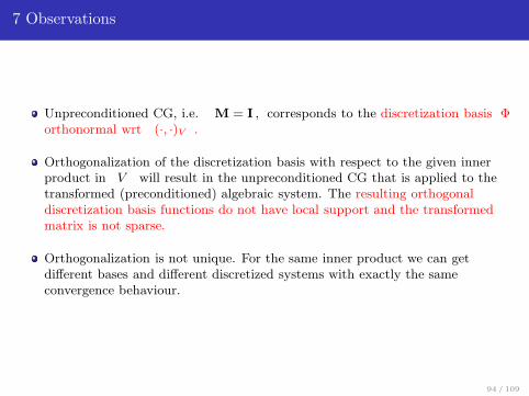
7 Observations
Unpreconditioned CG, i.e. M = I , corresponds to the discretization basis Φorthonormal wrt (·, ·)V .
Orthogonalization of the discretization basis with respect to the given innerproduct in V will result in the unpreconditioned CG that is applied to thetransformed (preconditioned) algebraic system. The resulting orthogonaldiscretization basis functions do not have local support and the transformedmatrix is not sparse.
Orthogonalization is not unique. For the same inner product we can getdifferent bases and different discretized systems with exactly the sameconvergence behaviour.
94 / 109
7 Algebraic preconditioning?
Consider an algebraic preconditioning with the (SPD) preconditioner
M = LL∗ = L (QQ
∗) L∗
Where QQ∗ = Q∗Q = I .
Question: Can any algebraic preconditioning be expressed in the operatorpreconditioning framework? How does it link with the discretization and the choiceof the inner product in V ?
95 / 109
7 Change of the basis and of the inner product
Transform the discretization bases
Φ = Φ ((LQ)∗)−1, Φ# = Φ#LQ .
with the change of the inner product in V (recall (u, v)V = v∗Mu )
(u, v)new,V = (Φu, Φv)new,V := v∗u = v
∗LQQ
∗L
∗u = v
∗LL
∗u = v
∗Mu .
The discretized Hilbert space formulation of CG gives the algebraicallypreconditioned matrix formulation of CG with the preconditioner M
(more specifically, it gives the unpreconditioned CG applied to the algebraicallypreconditioned discretized system).
96 / 109
7 Sparsity, locality, global transfer of information
Sparsity of matrices of the algebraic systems is always presented as an advantage ofthe FEM discretizations.
Sparsity means locality of information in the individual matrix rows/columns.Getting a sufficiently accurate approximation to the solution may then requiremany matrix-vector multiplications (a large dimension of the Krylov space).
Preconditioning can be interpreted in part as addressing the unwanted consequenceof sparsity (locality of the supports of the basis functions). Globally supportedbasis functions (hierarchical bases preconditioning, DD with coarse spacecomponents, multilevel methods, hierarchical grids etc.) can efficiently handle thetransfer of global information.
97 / 109

7 Example - Nonhomogeneous diffusion tensor
0 5 10 15 20 25 30 35 4010
−3
10−2
10−1
100
101
102
103
104
Squared energy norm of the algebraic error
P1 FEM ; cond =2.57e+03P1 FEM ichol ; cond =2.67e+01P1 FEM lapl ; cond =1.00e+02P1 FEM ichol(1e−02) ; cond =1.72e+00
PCG convergence: unpreconditioned; ichol (no fill-in); Laplace operatorpreconditioning; ichol (drop-off tolerance 1e-02). Uniform mesh, condition numbers
2.5e03, 2.6e01, 1.0e02, 1.7e00.
98 / 109

7 Transformed basis elements
−1
0
1
−1
0
10
0.25
0.5
0.75
1
Discretization basis function: P1 FEM; nnz = 1
−1
0
1
−1
0
10
0.02
0.04
0.06
Discretization basis function: P1 FEM ichol; nnz = 5
Original discretization basis element and its transformation corresponding to theichol preconditioning.
99 / 109
7 Transformed basis elements
−1
0
1
−1
0
10
0.2
0.4
0.6
0.8
Discretization basis function: P1 FEM lapl; nnz = 225
−1
0
1
−1
0
10
0.02
0.04
0.06
0.08
Discretization basis function: P1 FEM ichol(1e−02); nnz = 214
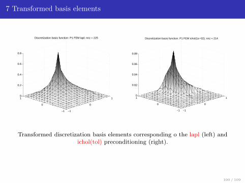
Transformed discretization basis elements corresponding o the lapl (left) andichol(tol) preconditioning (right).
100 / 109
8. HPC computations with Krylov subspace methods?
References
E. Carson, M. Rozloznık, Z.S., P, Tichy, and M. Tuma, On the numericalstability analysis of pipelined Krylov subspace methods, (2016, submitted forpublication).
101 / 109
9. Myths about Krylov subspace methods
Myth: A belief given uncritical acceptance by the members of a group especially insupport of existing or traditional practices and institutions.
Webster’s Third New International Dictionary, Enc. Britannica Inc., Chicago (1986)
102 / 109
9 Widespread statements that are misleading or plainly incorrect
1 Minimal polynomials and finite termination property
2 Chebyshev bounds and CG
3 Spectral information and clustering of eigenvalues
4 Operator-based bounds and functional analysis arguments on convergence
5 Finite precision computations can not be seen as a minor modification of theexact considerations
6 Linearization of nonlinear phenomenon without noticing that this eliminatesthe main principle behind the phenomenon, i.e. the adaptation to the problem
7 Short term recurrences can not guarantee well conditioned basis due torounding errors. This is true even for symmetric positive definite problems, andit remains true also for nonsymmetric problems
8 Sparsity can have positive as well as negative effects to computations
103 / 109
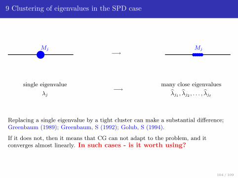
9 Clustering of eigenvalues in the SPD case
④Mj
−→ tttttMj
single eigenvalue
λj
−→many close eigenvalues
λj1 , λj2 , . . . , λjℓ
Replacing a single eigenvalue by a tight cluster can make a substantial difference;Greenbaum (1989); Greenbaum, S (1992); Golub, S (1994).
If it does not, then it means that CG can not adapt to the problem, and itconverges almost linearly. In such cases - is it worth using?
104 / 109
9 Minimal polynomials, asymptotics
It is not true that CG (or other Krylov subspace methods used for solvingsystems of linear algebraic equations with symmetric matrices) applied to amatrix with t distinct well separated tight clusters of eigenvalues produces ingeneral a large error reduction after t steps; see Sections 5.6.5 and 5.9.1 ofLiesen, S (2013). This myth has been disproved more than 20 years ago; seeGreenbaum (1989); S (1991); Greenbaum, S (1992). Still it is persistentlyrepeated in literature as an obvious fact.
With no information on the structure of invariant subspacesit is not true that distribution of eigenvalues provides insight intothe asymptotic behavior of Krylov subspace methods (such as GMRES)applied to systems with generally nonsymmetric matrices; see Sections 5.7.4,5.7.6 and 5.11 of Liesen, S (2013). As before, the relevant results Greenbaum, S(1994); Greenbaum, Ptak, S (1996) and Arioli, Ptak, S (1998) are (almost)twenty years old.
105 / 109
9 How the mathematical myths are created?
Rutishauser (1959) as well as Lanczos (1952) considered CG principallydifferent in their nature from the method based on the Chebyshev polynomials.
Daniel (1967) did not identify the CG convergence with the Chebyshevpolynomials-based bound. He carefully writes (modifyling slightly his notation)
“assuming only that the spectrum of the matrix A lies inside the interval[λ1, λN ], we can do no better than Theorem 1.2.2.”
That means that the Chebyshev polynomials-based bound holds for anydistribution of eigenvalues between λ1 and λ1 and for any distribution ofthe components of the initial residuals in the individual invariant subspaces.
Why we do not read the original works? They are many times most valuablesources of insight, that can be gradually forgotten and can be overshadowed bycommonly accepted myth ...
106 / 109
9 Analogy with a priori and a posteriori numerical PDE analysis
Think of a priori and a posteriori numerical PDE analysis!
The Chebyshev bound is a typical a priori bound; it uses no a posterioriinformation.
A priori bounds are useful for the purpose they have been derived to.They can not take over the role of the a posteriori bounds.
107 / 109
9 Concluding remarks and outlook
Krylov subspace methods adapt to the problem. Exploiting this adaptation isthe key to their efficient use.
Unlike in nonlinear problems and/or multilevel methods, analysis of Krylovsubspace methods can not be based, in general, on contraction arguments.
Individual steps modeling-analysis-discretization-computation should not beconsidered separately within isolated disciplines. They form a single problem.Operator preconditioning follows this philosophy.
Fast HPC computations require handling all involved issues.A posteriori error analysis and stopping criteria are essential ...
Assumptions must be honored
Historia Magistra Vitae
108 / 109

Thank you very much for your kind patience!
109 / 109