Matlab Basics Tutorial

This paper is a tutorial for the first part of the ECG370 L Control lab. Here we will learn how to write a Matlab code for creating a transfer function and then analyzing this transfer code for its reaction to several types of stimulus.

Vectors

Let's start off by creating something simple, like a vector. Enter each element of the vector (separated by a space) between brackets, and set it equal to a variable. For example, to create the vector a, enter into the Matlab command window (you can "copy" and "paste" from your browser into Matlab to make it easy):

a = [1 2 3 4 5 6 9 8 7]

Matlab should return: a = 1 2 3 4 5 6 9 8 7

Let's say you want to create a vector with elements between 0 and 20 evenly spaced in increments of 2 (this method is frequently used to create a time vector):

t = 0:2:20 t = 0 2 4 6 8 10 12 14 16 18 20

Manipulating vectors is almost as easy as creating them. First, suppose you would like to add 2 to each of the elements in vector 'a'. The equation for that looks like:

b = a + 2 b = 3 4 5 6 7 8 11 10 9

Now suppose, you would like to add two vectors together. If the two vectors are the same length, it is easy. Simply add the two as shown below:

c = a + b c = 4 6 8 10 12 14 20 18 16

Subtraction of vectors of the same length works exactly the same way.

Functions

To make life easier, Matlab includes many standard functions. Each function is a block of code that accomplishes a specific task. Matlab contains all of the standard functions such as sin, cos, log, exp, sqrt, as well as many others. Commonly used constants such as pi, and i or j for the square root of -1, are also incorporated into Matlab.

sin(pi/4) ans =

0.7071

To determine the usage of any function, type help [function name] at the Matlab command window.

Matlab even allows you to write your own functions with the function command; follow the link to learn how to write your own functions and see a listing of the functions we created for this tutorial.

Plotting

It is also easy to create plots in Matlab. Suppose you wanted to plot a sine wave as a function of time. First make a time vector (the semicolon after each statement tells Matlab we don't want to see all the values) and then compute the sin value at each time.

t=0:0.25:7; y = sin(t); plot(t,y)

The plot contains approximately one period of a sine wave. Basic plotting is very easy in Matlab, and the plot command has extensive add-on capabilities. I would recommend you visit the plotting page to learn more about it.

Polynomials

In Matlab, a polynomial is represented by a vector. To create a polynomial in Matlab, simply enter each coefficient of the polynomial into the vector in descending order. For instance, let's say you have the following polynomial:

To enter this into Matlab, just enter it as a vector in the following manner

x = [1 3 -15 -2 9] x = 1 3 -15 -2 9

Matlab can interpret a vector of length n+1 as an nth order polynomial. Thus, if your polynomial is missing any coefficients, you must enter zeros in the appropriate place in the vector. For example,

would be represented in Matlab as:

y = [1 0 0 0 1]

You can find the value of a polynomial using the polyval function. For example, to find the value of the above polynomial at s=2,

z = polyval([1 0 0 0 1],2) z = 17

You can also extract the roots of a polynomial. This is useful when you have a high-order polynomial such as

Finding the roots would be as easy as entering the following command;

roots([1 3 -15 -2 9]) ans = -5.5745 2.5836 -0.7951 0.7860

Let's say you want to multiply two polynomials together. The product of two polynomials is found by taking the convolution of their coefficients. Matlab's function conv that will do this for you.

x = [1 2]; y = [1 4 8]; z = conv(x,y) z = 1 6 16 16

Dividing two polynomials is just as easy. The deconv function will return the remainder as well as the result. Let's divide z by y and see if we get x.

[xx, R] = deconv(z,y) xx = 1 2 R = 0 0 0 0

As you can see, this is just the polynomial/vector x from before. If y had not gone into z evenly, the remainder vector would have been something other than zero.

If you want to add two polynomials together which have the same order, a simple z=x+y will work (the vectors x and y must have the same length). In the general case, the user-defined function, polyadd can be used. To use polyadd, copy the function into an m-file, and then use it just as you would any other function in the Matlab toolbox. Assuming you had the polyadd function stored as a m-file, and you wanted to add the two uneven polynomials, x and y, you could accomplish this by entering the command:

z = polyadd(x,y) x = 1 2 y = 1 4 8 z = 1 5 10

Matrices

Entering matrices into Matlab is the same as entering a vector, except each row of elements is separated by a semicolon (;) or a return:

B = [1 2 3 4;5 6 7 8;9 10 11 12] B = 1 2 3 4 5 6 7 8 9 10 11 12 B = [ 1 2 3 4 5 6 7 8 9 10 11 12] B = 1 2 3 4 5 6 7 8 9 10 11 12

Matrices in Matlab can be manipulated in many ways. For one, you can find the transpose of a matrix using the apostrophe key:

C = B' C = 1 5 9 2 6 10 3 7 11 4 8 12

It should be noted that if C had been complex, the apostrophe would have actually given the complex conjugate transpose. To get the transpose, use .' (the two commands are the same if the matix is not complex).

Now you can multiply the two matrices B and C together. Remember that order matters when multiplying matrices.

D = B * C D = 30 70 110 70 174 278 110 278 446 D = C * B D = 107 122 137 152 122 140 158 176 137 158 179 200 152 176 200 224

Another option for matrix manipulation is that you can multiply the corresponding elements of two matrices using the .* operator (the matrices must be the same size to do this).

E = [1 2;3 4] F = [2 3;4 5] G = E .* F E = 1 2 3 4 F = 2 3 4 5 G = 2 6 12 20

If you have a square matrix, like E, you can also multiply it by itself as many times as you like by raising it to a given power.

E^3 ans = 37 54 81 118

If wanted to cube each element in the matrix, just use the element-by-element cubing. E.^3 ans = 1 8 27 64

You can also find the inverse of a matrix: X = inv(E)

X = -2.0000 1.0000 1.5000 -0.5000

or its eigenvalues: eig(E) ans = -0.3723 5.3723

There is even a function to find the coefficients of the characteristic polynomial of a matrix. The "poly" function creates a vector that includes the coefficients of the characteristic polynomial.

p = poly(E) p = 1.0000 -5.0000 -2.0000

Remember that the eigenvalues of a matrix are the same as the roots of its characteristic polynomial: roots(p) ans = 5.3723 -0.3723

Printing

Printing in Matlab is pretty easy. Just follow the steps illustrated below:

Macintosh

To print a plot or a m-file from a Macintosh, just click on the plot or m-file, select Print under the File menu, and hit return.

Windows To print a plot or a m-file from a computer running Windows, just selct Print from the File menu in the window of the plot or m-file, and hit return.

Unix To print a plot on a Unix workstation enter the command: print -P<printername> If you want to save the plot and print it later, enter the command: print plot.ps Sometime later, you could print the plot using the command "lpr -P plot.ps" If you are using a HP workstation to print, you would instead use the command "lpr -d plot.ps"

To print a m-file, just print it the way you would any other file, using the command "lpr -P <name of m-file>.m" If you are using a HP workstation to print, you would instead use the command "lpr -d plot.ps<name of m-file>.m"

Using M-files in Matlab

There are slightly different things you need to know for each platform.

Macintosh

There is a built-in editor for m-files; choose "New M-file" from the File menu. You can also use any other editor you like (but be sure to save the files in text format and load them when you start Matlab).

Windows

Running Matlab from Windows is very similar to running it on a Macintosh. However, you need to know that your m-file will be saved in the clipboard. Therefore, you must make sure that it is saved as filename.m

Unix

You will need to run an editor separately from Matlab. The best strategy is to make a directory for all your m-files, then cd to that directory before running both Matlab and the editor. To start Matlab from your Xterm window, simply type: matlab.

You can either type commands directly into matlab, or put all of the commands that you will need together in an m-file, and just run the file. If you put all of your m-files in the same directory that you run matlab from, then matlab will always find them.

Getting help in Matlab

Matlab has a fairly good on-line help; type help commandname

for more information on any given command. You do need to know the name of the command that you are looking for; a list of the all the ones used in these tutorials is given in the command listing; a link to this page can be found at the bottom of every tutorial and example page.

Here are a few notes to end this tutorial.

You can get the value of a particular variable at any time by typing its name.

B B = 1 2 3 4 5 6 7 8 9 You can also have more that one statement on a single line, so long as you separate them with either a semicolon or comma.

Also, you may have noticed that so long as you don't assign a variable a specific operation or result, Matlab with store it in a temporary variable called "ans".

TRANSFER FUNCTION: The purpose of a transfer function (TF) should be covered in lecture class. Here, we will only work with the mechanics of the TF and how to manipulate one for the purpose of analyzing a system. In this case today the system will be an electric circuit, but be aware this represents only a small fraction of the types of systems that are represented by transfer functions. For our purposes at this time a TF is a s space function that represents the zeros and poles of a system in the s plane. They have the general format of : System Function (s) = (Asn-1 + Bsn-2 +… Ms + N) (Psn+ Qs n-1+ …Xs + Y) It should be noted that in class you were taught that the order of the numerator should be less than that of the denominator. Please adhere to this restriction for this class, but note that Matlab will often accept any transfer function. In Matlab, like any programming language, the computer will do what it is told. It will create any TF, but it is up to you to make sure that the TF created is a valid one and the one you desire. The TF created is a ratio of polynomial coefficient arrays. That is, one creates the denominator and the numerator by creating an array then the computer binds them with a “create a transfer function command”. To create the coefficient array one looks at the s function for the numerator. One uses the coefficients for the array elements. For example the s function : N(s) = 1 s4 + 2s3 + 5s + 1 would have a coefficient array of num=[ 1 2 0 5 1] . Obviously the s2 term is not existent in the given function so its coefficient is 0. Next we wish to create the den array. Let us assume a s function of: D(s) = 2 s3 + 7s2 + 1s + 3 would have a coefficient array of den=[ 2 7 1 3] . The underlined and italicized portions are the actual Matlab commands used to create the arrays. To use these arrays to create a TF we simply use the TF function. Of course one must store this information in some location; here we will use the variable sys. The command would look like: sys = tf(num,den) Matlab would then display the TF in the following manner: Transfer function: s^4 + 2 s^3 + 5 s + 1 --------------------- 2 s^3 + 7 s^2 + s + 3 No attention to the propriety of the TF has yet been made. Recall that for the function to be proper the poles must all exist on the left hand side (- side). Let us check the poles and zeros of our made up system. The command to check the poles and zeros of the TF are the commands pole and zero. For example the Matlab program would return the following responses: zero(sys) ans = -2.6556

0.4264 + 1.3143i 0.4264 - 1.3143i -0.1972 pole(sys) ans = -3.4802 -0.0099 + 0.6564i -0.0099 - 0.6564i One can quickly see that the transfer function does not describe a proper system. Although this is the method suggested for a control application, the same effect can be realized using a more general term roots for any polynomial. roots(den) ans = -3.4802 -0.0099 + 0.6564i -0.0099 - 0.6564i This gives the same results as the pole command which finds the roots of the denominator for the TF. ANALYSIS: Analysis of a circuit means finding its response to a stimulus. The response is usually determined in terms of numerical data or graphically. Either representation is available through Matlab. Here we will look at graphical results. The first process we will look at is the response of a circuit subjected to a step function. We will use the following transfer function which will be referred to as syt2. 6 s2 + 1 --------------------- s3 + 3 s2 + 3 s + 1 Using the method outlined above create this TF. The simplest method to use to generate the response of a step function on the system is with the command: step(syt2)

You will create a graph such as:

st

There is a great deal of information provided in this graph, and a great deal more can be derived from this graph if one uses the tools available in the figure menu. The three mocommon desired characteristics are the overshoot, undershoot and the settling time. There are several methods to determine these parameters, but here we will try to

just label the points and hand calculate them.

In the figure menu choose Tools and then make sure the Data Cursor is checked. As you move your cursor around the graph the cursor will take the shape of a cross. Place the cross on the highest point, then the lowest point and where the solid (data) line and the dotted line finally meet, then left click the cursor. This will place a label on the graph at that point. The result will be similar to the following.

This is not the automatic reading method for these results, but one can take the data from this graph to hand calculate the results. Once the root locus section is reached a tutorial for determining such parameters for that purpose will be discussed. Try similar graphs with the impulse command.

STEP(SYS) plots the step response of the LTI model SYS. STEP(SYS,TFINAL) simulates the step response from t=0 to the final time t=TFINAL. For discrete-time models with unspecified sampling time, TFINAL is interpreted as the number of samples. STEP(SYS1,SYS2,...,T) plots the step response of multiple LTI models SYS1,SYS2,... on a single plot. The time vector T is optional. You can also specify a color, line style, and marker for each system, as in step(sys1,'r',sys2,'y--',sys3,'gx'). What this function does is to show the response of the system to a unit step input. It can be used with any system including electronic circuits. Let us use the following transfer function: s^2 + 2 s + 3 --------------------- s^3 + 2 s^2 + 3 s + 4 This is an arbitrary TF, however it exhibits some interesting characteristics. We will then execute the command step (sys) The following graph appears.

0 5 10 15 20 25 300

0.2

0.4

0.6

0.8

1

1.2

1.4Step Response

Time (sec)

Ampl

itude

A Pspice simulation of the same circuit would yield the same results if you knew a circuit with this TF. Once you have this graph, you can annotate it with labels and plot points. From these points you can calculate the frequency of oscillation and other interesting characteristics. The process for such characteristics as rise time and settling time is by pressing the right mouse button and selecting the desired function. On the graph points will appear on the plot. These dots represent such characteristics as rise time, settling time and so on. By left clinking on the dot the information will appear. An example of this is provided in the graph below. Sometimes you are only interested in a specific time period starting from 0. In that case you should use the format STEP(SYS,TFINAL). This simulates the step response from t=0 to the final time t=TFINAL.

Although a Pspice simulation can be used to obtain similar information, this program will yield results for systems that have transfer functions not derived from electronic circuits. Keep in mind that as a percentage, electronics is only a small fraction of the applications of Controls. Because of this once the Transfer Function has been determined; no other circuitry considerations will be used. The step function is only one of the options available. Another function is the impulse function: IMPULSE(SYS) plots the impulse response of the LTI model SYS (created with either TF, ZPK, or SS). The time range and number of points are chosen automatically. For continuous systems with direct feed through, the infinite pulse at t=0 is disregarded. IMPULSE(SYS,TFINAL) simulates the impulse response from t=0 to the final time t=TFINAL. For discrete-time systems with unspecified sampling time, TFINAL is interpreted as the number of samples. IMPULSE(SYS,T) uses the user-supplied time vector T for simulation. For discrete-time models, T should be of the form Ti:Ts:Tf where Ts is the sample time. For continuous-time models, T should be of the form Ti:dt:Tf where dt will become the sample time of a discrete approximation to the continuous system. The impulse is always assumed to arise at t=0 (regardless of Ti). It should be noted that the impulse itself is a simulated stimulation of infinite intensity for a time of 0 duration. Although this is impossible in reality, recall that the transfer function can be determined from the impulse response. A command of impulse (sys) will give the results shown below:

Again certain properties can be displayed on the graph by right clicking the pointer on the curve itself. Step and impulse are vital tools in controls. You will use them often. Beyond the step and impulse functions are functions that are more common to your electronics background. These would be a sine wave, triangle wave, square wave and some mix of these various functions. It is also possible to create the response to these or any arbitrary function using Matlab using the LSIM function. LSIM Simulate time response of LTI models to arbitrary inputs. LSIM(SYS,U,T) plots the time response of the LTI model SYS to the input signal described by U and T. The time vector T consists of regularly spaced time samples and U is a matrix with as many columns as inputs and whose i-th row specifies the input value at time T(i). For example, t = 0:0.01:5; u = sin(t); lsim(sys,u,t) Simulates the response of a single-input model SYS to the input u(t)=sin(t) during 5 seconds.

Using the same transfer function as above, you should display the following figure

Although this figure is in itself uninteresting there are certain aspects that are important. First note that the system has an initial value, and the initial response differs from the steady state response. The power of this function is that any input signal can be simulated. The above response is that of a sine wave. We could just as easily constructed a triangle wave and used it as a input stimulus. Impulse and Step are very important commands in Matlab. In motor control, one wishes to provide a step function as a simulation to the turning on of the motor. Impulse functions reveal information concerning the TF of the system. Often, a different or maybe unusual stimulus is required. In this case one would wish to create a waveform. For a simulation with an arbitrary input one would use the lsim command. lsim simulates the (time) response of continuous or discrete linear systems to arbitrary inputs. When invoked without left-hand arguments, lsim plots the response on the screen. lsim(sys,u,t) produces a plot of the time response of the LTI model sys to the input time history t,u. The vector t specifies the time samples for the simulation and consists of regularly spaced time samples. t = 0:dt:Tfinal The matrix u must have as many rows as time samples (length(t)) and as many columns as system inputs. Each row u(i,:) specifies the input value(s) at the time sample t(i). Obviously it is necessary to create the u and t matrix first. For this the command gensig is used

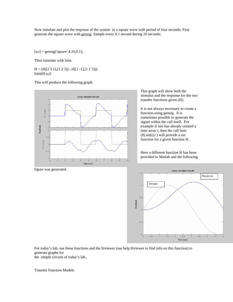
Now simulate and plot the response of the system to a square wave with period of four seconds. First enerate the square wave with gensigg . Sample every 0.1 second during 10 seconds:

,0.1);

= [tf([2 5 1],[1 2 3]) ; tf([1 -1],[1 1 5])]

imulus and the response for the two

a me array t, then the call lsim

(t),t ) will provide a sin

gure was generated.

the ltiviewer (use help ltiviewer to find info on this function) to enerate graphs for e simple circuits of today’s lab..

ransfer Function Models

[u,t] = gensig('square',4,10 Then simulate with lsim. Hlsim(H,u,t) This will produce the following graph.

This graph will show both the sttransfer functions given (H). It is not always necessary to create a function using gensig. It is sometimes possible to generate the signal within the call itself. For example if one has already createdti(H,sinfunction for a given function H.

Here a different function H has been provided to Matlab and the following

fi For today’s lab, use these functions andgth T

This section explains how to specify continuous-time SISO and MIMO transfer function models. The specification of discrete-time transfer function models is a simple extension of the continuous-time case

ee Discrete-Time Models). In this section you can also read about how to specify transfer functions

ISO Transfer Function Models

here are two ways to specify SISO transfer functions: Using the tf command As rational expressions in

o specify a SISO transfer function model using the tf command, type = tf(num,den)

ting the coefficients of the polynomials and , respectively, when ese polynomials are ordered in descending powers of s. The resulting variable h is a TF object containing

, you can create the transfer function

y typing = tf([1 0],[1 2 10])

AB responds with tion:

------------ 2 + 2 s + 10

so specify transfer functions as rational expressions in the Laplace variable s by: Defining the ariable s as a special TF model

on in s

or example, once s is defined with tf as in 1, = s/(s^2 + 2*s +10);

roduces the same transfer function as = tf([1 0],[1 2 10]);

(sconsisting of pure gains. S A continuous-time SISO transfer function is characterized by its numerator and denominator , both polynomials of the Laplace variable s. Tthe Laplace variable s Th where num and den are row vectors lisththe numerator and denominator data. For example bh MATLTransfer func s --s^ Note the customized display used for TF objects. You can alvs = tf('s'); Entering your transfer function as a rational expressi FH ph

freqresp

e frequency response over grid of frequencies

= freqresp(sys,w)

escription

s,w) turns a 3-D array H with the frequency as the last dimension (see "Arguments" below). For LTI arrays of

continuous time, the response at a frequency is the transfer function value at . For state-space models,

discrete time, the real frequencies w(1),..., w(N) are mapped to points on the unit circle using the

here is the sample time. The transfer function is then evaluated at the resulting values. The default is odels with unspecified sample time.

emark

sys is an FRD model, freqresp(sys,w), w can only include frequencies in sys.frequency. Interpolation and re not supported. To interpolate an FRD model, use interp.

rguments

systems, H(1,1,k) gives the scalar response at the frequency w(k). For MIMO systems, the equency response at w(k) is H(:,:,k), a matrix with as many rows as outputs and as many columns as

xample

Comput Syntax H D H = freqresp(sys,w) computes the frequency response of the LTI model sys at the real frequency points specified by the vector w. The frequencies must be in radians/sec. For single LTI Models, freqresp(syresize [Ny Nu S1 ... Sn], freqresp(sys,w) returns a [Ny-by-Nu-by-S1-by-...-by-Sn] length (w) array. Inthis value is given by Intransformation wused for m R Ifextrapolation a A The output argument H is a 3-D array with dimensions For SISOfrinputs. E

Compute the frequency response of

Type 00]

= freqresp(P,w)

0 0.5000- 0.5000i 0.2000+ 0.6000i 1.0000

0 0.0099- 0.0990i 0.9423+ 0.2885i 1.0000

0 0.0001- 0.0100i 0.9994+ 0.0300i 1.0000

e three displayed matrices are the values of for

in the 3-D array H is relative to the frequency vector w, so you can extract the frequency sponse at rad/sec by

==10)

0 0.0099- 0.0990i 0.9423+ 0.2885i 1.0000

lgorithm

or transfer functions or zero-pole-gain models, freqresp evaluates the numerator(s) and denominator(s) at

h frequency oint, taking advantage of the Hessenberg structure. The reduction to Hessenberg form provides a good

between efficiency and reliability. See [1] for more details on this technique.

iagnostics

the system has a pole on the axis (or unit circle in the discrete-time case) and w happens to contain this equency point, the gain is infinite, is singular, and freqresp produces the following warning message.

at the frequencies . w = [1 10 1HH(:,:,1) = - H(:,:,2) = H(:,:,3) = Th The third indexreH(:,:,w ans = A Fthe specified frequency points. For continuous-time state-space models , the frequency response is For efficiency, is reduced to upper Hessenberg form and the linear equation is solved at eacpcompromise D Iffr bode

Compute the Bode frequency response of LTI models

ode(sys)

ode(sys1,sys2,...,sysN,w) N,'PlotStyleN')

ag,phase,w] = bode(sys)

escription

),

ted as 20log10, where is the system's equency response. Bode plots are used to analyze system properties such as the gain margin, phase

rete, e MIMO case, bode produces an array of Bode plots, each plot showing the Bode

sponse of one particular I/O channel. The frequency range is determined automatically based on the

us on ax}. To use particular frequency points,

t w to the vector of desired frequencies. Use logspace to generate logarithmically spaced frequency

ngle figure. All systems must have the same number of inputs and outputs, but may otherwise be a mix of

sysN,'PlotStyleN') specifies which color, linestyle, and/or marker should be used plot each system. For example,

ode(sys1,'r--',sys2,'gx')

ys1 and green 'x' markers for the second system sys2.

ments ag,phase,w] = bode(sys) ag,phase] = bode(sys,w)

Syntax bbode(sys,w) bode(sys1,sys2,...,sysN) bbode(sys1,'PlotStyle1',...,sys [m D bode computes the magnitude and phase of the frequency response of LTI models. When invoked withoutleft-side arguments, bode produces a Bode plot on the screen. The magnitude is plotted in decibels (dBand the phase in degrees. The decibel calculation for mag is compufrmargin, DC gain, bandwidth, disturbance rejection, and stability. bode(sys) plots the Bode response of an arbitrary LTI model sys. This model can be continuous or discand SISO or MIMO. In thresystem poles and zeros. bode(sys,w) explicitly specifies the frequency range or frequency points to be used for the plot. To foca particular frequency interval [wmin,wmax], set w = {wmin,wmsevectors. All frequencies should be specified in radians/sec. bode(sys1,sys2,...,sysN) or bode(sys1,sys2,...,sysN,w) plots the Bode responses of several LTI models on a sicontinuous and discrete systems. This syntax is useful to compare the Bode responses of multiple systems. bode(sys1,'PlotStyle1',...,tob uses red dashed lines for the first system s When invoked with left-side argu[m[m

return the magnitude and phase (in degrees) of the frequency response at the frequencies w (in rad/sec). he outputs mag and phase are 3-D arrays with the frequency as the last dimension (see "Arguments" elow for details). You can convert the magnitude to decibels by

20*log10(mag)

emark

sys is an FRD model, bode(sys,w), w can only include frequencies in sys.frequency.

rguments

he output arguments mag and phase are 3-D arrays with dimensions

tems are treated as arrays of SISO systems and the magnitudes and phases are computed for each ISO entry hij independently (hij is the transfer function from input j to output i). The values mag(i,j,k) and hase(i,j,k) then characterize the response of hij at the frequency w(k).

xample

plot the Bode response of the continuous SISO system

typing = tf([1 0.1 7.5],[1 0.12 9 0 0]);

o plot the response on a wider frequency range, for example, from 0.1 to 100 rad/sec, type

ou can also discretize this system using zero-order hold and the sample time second, and compare the ntinuous and discretized responses by typing

d = c2d(g,0.5) ,'b--')

r continuous-time systems, bode computes the frequency response by evaluating the transfer function on e imaginary axis . Only positive frequencies are considered. For state-space models, the frequency

Tbmagdb = R If A T For SISO systems, mag(1,1,k) and phase(1,1,k) give the magnitude and phase of the response at the frequency = w(k). MIMO sysSp E You can bygbode(g) Tbode(g,{0.1 , 100}) Ycogbode(g,'r',gd Algorithm Fothresponse is

When numerically safe, is diagonalized for maximum speed. Otherwise, is reduced to upper Hessenberg

cy and liability. See [1] for more details on this technique.

ponse is obtained by evaluating the transfer function on the nit circle. To facilitate interpretation, the upper-half of the unit circle is parametrized as

here is the sample time. is called the Nyquist frequency. The equivalent "continuous-time frequency" is

periodic with period , bode plots the response only up to the Nyquist frequency . If the sample time is nspecified, the default value is assumed.

the system has a pole on the axis (or unit circle in the discrete case) and w happens to contain this equency point, the gain is infinite, is singular, and bode produces the warning message ingularity in freq. response due to jw-axis or unit circle pole.

form and the linear equation is solved at each frequency point, taking advantage of the Hessenberg structure. The reduction to Hessenberg form provides a good compromise between efficienre For discrete-time systems, the frequency resu wthen used as the -axis variable. Because isu Diagnostics IffrS nichols

ols frequency response of LTI models

yntax

ichols(sys1,'PlotStyle1',...,sysN,'PlotStyleN')

ag,phase,w] = nichols(sys) = nichols(sys,w)

ichols(sys) produces a Nichols plot of the LTI model sys. This model can be continuous or discrete, SISO

Compute Nich S nichols(sys) nichols(sys,w) nichols(sys1,sys2,...,sysN) nichols(sys1,sys2,...,sysN,w) n [m[mag,phase] Description nichols computes the frequency response of an LTI model and plots it in the Nichols coordinates. Nichols plots are useful to analyze open- and closed-loop properties of SISO systems, but offer little insight into MIMO control loops. Use ngrid to superimpose a Nichols chart on an existing SISO Nichols plot. nor MIMO. In the MIMO case, nichols produces an array of Nichols plots, each plot showing the response

of one particular I/O channel. The frequency range and gridding are determined automatically basesystem poles and zeros.

d on the

y

ichols(sys1,sys2,...,sysN) or nichols(sys1,sys2,...,sysN,w) superimposes the Nichols plots of several LTI odels on a single figure. All systems must have the same number of inputs and outputs, but may

therwise be a mix of continuous- and discrete-time systems. You can also specify a distinctive color, each system plot with the syntax

ichols(sys1,'PlotStyle1',...,sysN,'PlotStyleN')

ee bode for an example.

hen invoked with left-hand arguments,

turn the magnitude and phase (in degrees) of the frequency response at the frequencies w (in rad/sec). he outputs mag and phase are 3-D arrays similar to those produced by bode (see the bode reference page).

sponse of the system um = [-4 48 -18 250 600]; en = [1 30 282 525 60]; = tf(num,den)

ichols(H); ngrid

he right-click menu for Nichols plots includes the Tight option under Zoom. You can use this to clip nbounded branches of the Nichols plot.

____________________________________________________

r LTI system response analysis

nichols(sys,w) explicitly specifies the frequency range or frequency points to be used for the plot. To focus on a particular frequency interval [wmin,wmax], set w = {wmin,wmax}. To use particular frequencpoints, set w to the vector of desired frequencies. Use logspace to generate logarithmically spaced frequency vectors. Frequencies should be specified in radians/sec. nmolinestyle, and/or marker forn S W[mag,phase,w] = nichols(sys) [mag,phase] = nichols(sys,w) reTThey have dimensions Example Plot the Nichols rendH n Tu _______ ltiview Initialize an LTI Viewer fo Syntax

ltiview ltiview(sys1,sys2,...,sysn)

iview('plottype',sys1,sys2,...,sysn) iview('plottype',sys,extras)

',viewers) iview('current',sys1,sys2,...,sysn,viewers)

escription

ed without input arguments, initializes a new LTI Viewer for LTI system response

iview(sys1,sys2,...,sysn) opens an LTI Viewer containing the step response of the LTI models s1,sys2,...,sysn. You can specify a distinctive color, line style, and marker for each system, as in s1 = rss(3,2,2);

('plottype',sys) initializes an LTI Viewer containing the LTI response type indicated by plottype for odel sys. The string plottype can be any one of the following:

zmap'

yquist' ols'

igma'

r,

ample, iview({'step';'nyquist'},sys)

rguments supported by the various LTI model assed to the ltiview command.

xtras is one or more input arguments as specified by the function named in plottype. These arguments may e required or optional, depending on the type of LTI response. For example, if plottype is 'step' then extras

ltltltiview('clearlt D ltiview when invokanalysis. ltsysysys2 = rss(4,2,2); ltiview(sys1,'r-*',sys2,'m--'); ltiviewthe LTI m'step' 'impulse' 'initial' 'lsim' 'p'bode''n'nich's o plottype can be a cell vector containing up to six of these plot types. For exlt displays the plots of both of these response types for a given system sys. ltiview(plottype,sys,extras) allows the additional input aresponse functions to be p ebmay be the desired final time, Tfinal, as shown below. ltiview('step',sys,Tfinal)

However, if plottype is 'initial', the extras arguments must contain the initial conditions x0 and may contain

al',sys,x0,Tfinal)

iview('clear',viewers) clears the plots and data from the LTI Viewers with handles viewers.

ewers) adds the responses of the systems sys1,sys2,...,sysn to the LTI do not have the same I/O dimensions as those

er is first cleared and only the new responses are shown.

inally, iview(plottype,sys1,sys2,...sysN)

zes an LTI Viewer containing the responses of multiple LTI models, using the plot styles in yle, when applicable. See the individual reference pages of the LTI response functions for more

formation on specifying plot styles.

other arguments, such as Tfinal. ltiview('initi See the individual references pages of each possible plottype commands for a list of appropriate argumentsfor extras. lt ltiview('current',sys1,sys2,...,sysn,viViewers with handles viewers. If these new systems currently in the LTI Viewer, the LTI View Fltltiview(plottype,sys1,PlotStyle1,sys2,PlotStyle2,...) ltiview(plottype,sys1,sys2,...sysN,extras) initiali

lotStPin lsim Simulate LTI model response to arbitrary inputs

im(sys,u,t,x0,'foh')

im(sys1,sys2,...,sysN,u,t) ys2,...,sysN,u,t,x0)

im(sys1,'PlotStyle1',...,sysN,'PlotStyleN',u,t)

,t,x] = lsim(sys,u,t,x0)

im(sys)

escription

e (time) response of continuous or discrete linear systems to arbitrary inputs. When voked without left-hand arguments, lsim plots the response on the screen.

Syntax lsim(sys,u,t) lsim(sys,u,t,x0) lsim(sys,u,t,x0,'zoh') ls lslsim(sys1,sls [y ls D lsim simulates thin

lsim(sys,u,t) produces a plot of the time response of the LTI model sys to the input time history t,u. The

he LTI model sys can be continuous or discrete, SISO or MIMO. In discrete time, u must be sampled at

ime sampling dt=t(2)-t(1) is used to discretize the continuous model. If dt is too large ndersampling), lsim issues a warning suggesting that you use a more appropriate sample time, but will

r the system states. This syntax applies only to ate-space models.

ys,u,t,x0,'foh') explicitly specifies how the input values should be interpolated etween samples (zero-order hold or linear interpolation). By default, lsim selects the interpolation method utomatically based on the smoothness of the signal U.

mulates the responses of several LTI models to the same input history t,u and plots these responses on a ngle figure. As with bode or plot, you can specify a particular color, linestyle, and/or marker for each

im(sys1,'y:',sys2,'g--',u,t,x0)

ode or step.

hen invoked with left-hand arguments, ,t] = lsim(sys,u,t)

turn the output response y, the time vector t used for simulation, and the state trajectories x (for state-

tes. input data is undersampled (see

lgorithm).

im(sys), with no additional arguments, opens the Linear Simulation Tool, which affords greater flexibility specifying input signals and initial conditions. See Specifying Input Signals and Input Conditions in

x for more information.

vector t specifies the time samples for the simulation and consists of regularly spaced time samples. t = 0:dt:Tfinal The matrix u must have as many rows as time samples (length(t)) and as many columns as system inputs. Each row u(i,:) specifies the input value(s) at the time sample t(i). Tthe same rate as the system (t is then redundant and can be omitted or set to the empty matrix). In continuous time, the t(uuse the specified sample time. See Algorithm for a discussion of sample times. lsim(sys,u,t,x0) further specifies an initial condition x0 fost lsim(sys,u,t,x0,'zoh') or lsim(sba Finally, lsim(sys1,sys2,...,sysN,u,t) sisisystem, for example, ls The multisystem behavior is similar to that of b W[y[y,t,x] = lsim(sys,u,t) % for state-space models only [y,t,x] = lsim(sys,u,t,x0) % with initial state respace models only). No plot is drawn on the screen. The matrix y has as many rows as time samples (length(t)) and as many columns as system outputs. The same holds for x with "outputs" replaced by staNote that the output t may differ from the specified time vector when the A lsinGetting Started with the Control System Toolbo Example

Simulate and plot the response of the system

a square wave with period of four seconds. First generate the square wave with gensig. Sample every 0.1

hen simulate with lsim. 1],[1 2 3]) ; tf([1 -1],[1 1 5])]

im(H,u,t)

iscrete-time systems are simulated with ltitr (state space) or filter (transfer function and zero-pole-gain).

ms are discretized with c2d using either the 'zoh' or 'foh' method ('foh' is used for ooth input signals and 'zoh' for discontinuous signals such as pulses or square waves). The sampling

period can drastically affect simulation results. To illustrate why, consider the

its response to a square wave with period 1 second, you can proceed as follows: 2 = 62.83^2 = tf(w2,[1 2 w2]) = 0:0.1:5; % vector of time samples

im evaluates the specified sample time, gives this warning undersampled. Sample every 0.016 sec or

ster.

this response, discretize using the recommended sampling period: t=0.016;

0:dt:5; s = (rem(ts,1)>=0.5)

im(hd,us,ts)

his response exhibits strong oscillatory behavior hidden from the undersampled version.

tosecond during 10 seconds: [u,t] = gensig('square',4,10,0.1); TH = [tf([2 5ls Algorithm D Continuous-time systesmperiod is set to the spacing dt between the user-supplied time samples t. The choice of sampling second-order model To simulatewht u = (rem(t,1)>=0.5); % square wave values lsim(h,u,t) lsWarning: Input signal isfa and produces this plot. To improve ondts=uhd = c2d(h,dt) ls T lsim

Simulate LTI model response to arbitrary inputs

im(sys,u,t,x0,'foh')

im(sys1,sys2,...,sysN,u,t) ys2,...,sysN,u,t,x0)

im(sys1,'PlotStyle1',...,sysN,'PlotStyleN',u,t)

,t,x] = lsim(sys,u,t,x0)

im(sys)

escription

e (time) response of continuous or discrete linear systems to arbitrary inputs. When voked without left-hand arguments, lsim plots the response on the screen.

im(sys,u,t) produces a plot of the time response of the LTI model sys to the input time history t,u. The

he LTI model sys can be continuous or discrete, SISO or MIMO. In discrete time, u must be sampled at

ime sampling dt=t(2)-t(1) is used to discretize the continuous model. If dt is too large ndersampling), lsim issues a warning suggesting that you use a more appropriate sample time, but will

r the system states. This syntax applies only to ate-space models.

ys,u,t,x0,'foh') explicitly specifies how the input values should be interpolated etween samples (zero-order hold or linear interpolation). By default, lsim selects the interpolation method utomatically based on the smoothness of the signal U.

Syntax lsim(sys,u,t) lsim(sys,u,t,x0) lsim(sys,u,t,x0,'zoh') ls lslsim(sys1,sls [y ls D lsim simulates thin lsvector t specifies the time samples for the simulation and consists of regularly spaced time samples. t = 0:dt:Tfinal The matrix u must have as many rows as time samples (length(t)) and as many columns as system inputs. Each row u(i,:) specifies the input value(s) at the time sample t(i). Tthe same rate as the system (t is then redundant and can be omitted or set to the empty matrix). In continuous time, the t(uuse the specified sample time. See Algorithm for a discussion of sample times. lsim(sys,u,t,x0) further specifies an initial condition x0 fost lsim(sys,u,t,x0,'zoh') or lsim(sba Finally, lsim(sys1,sys2,...,sysN,u,t)

simulates the responses of several LTI models to the same input history t,u and plots these responses on a ngle figure. As with bode or plot, you can specify a particular color, linestyle, and/or marker for each

--',u,t,x0)

he multisystem behavior is similar to that of bode or step.

any rows as time samples ength(t)) and as many columns as system outputs. The same holds for x with "outputs" replaced by states.

he output t may differ from the specified time vector when the input data is undersampled (see lgorithm).

the Linear Simulation Tool, which affords greater flexibility specifying input signals and initial conditions. See Specifying Input Signals and Input Conditions in

imulate and plot the response of the system

ds. First generate the square wave with gensig. Sample every 0.1 10 seconds:

,t] = gensig('square',4,10,0.1);

hen simulate with lsim. = [tf([2 5 1],[1 2 3]) ; tf([1 -1],[1 1 5])]

are simulated with ltitr (state space) or filter (transfer function and zero-pole-gain).

used for gnals and 'zoh' for discontinuous signals such as pulses or square waves). The sampling

acing dt between the user-supplied time samples t.

affect simulation results. To illustrate why, consider the r model

o simulate its response to a square wave with period 1 second, you can proceed as follows:

sisystem, for example, lsim(sys1,'y:',sys2,'g T When invoked with left-hand arguments, [y,t] = lsim(sys,u,t) [y,t,x] = lsim(sys,u,t) % for state-space models only [y,t,x] = lsim(sys,u,t,x0) % with initial state return the output response y, the time vector t used for simulation, and the state trajectories x (for state-space models only). No plot is drawn on the screen. The matrix y has as m(lNote that tA lsim(sys), with no additional arguments, opens inGetting Started with the Control System Toolbox for more information. Example S to a square wave with period of four seconsecond during[u THlsim(H,u,t) Algorithm Discrete-time systems Continuous-time systems are discretized with c2d using either the 'zoh' or 'foh' method ('foh' issmooth input siperiod is set to the sp The choice of sampling period can drasticallysecond-orde T

w2 = 62.83^2

(t,1)>=0.5); % square wave values im(h,u,t)

im evaluates the specified sample time, gives this warning

is plot.

improve on this response, discretize using the recommended sampling period: t=0.016;

s = (rem(ts,1)>=0.5)

im(hd,us,ts)

ory behavior hidden from the undersampled version.

+++++++++++++++++++++++++++++++++++++++++++++++++++++++++

enerate test input signals for lsim

,t] = gensig(type,tau)

escription

,t] = gensig(type,tau) generates a scalar signal u of class type and with period tau (in seconds). The

in'Sine wave.'square'Square wave.'pulse'Periodic pulse.

also specifies the time duration Tf of the signal and the spacing Ts between e time samples t.

h = tf(w2,[1 2 w2]) t = 0:0.1:5; % vector of time samples u = (remls lsWarning: Input signal is undersampled. Sample every 0.016 sec or faster. and produces th Todts=0:dt:5; uhd = c2d(h,dt) ls This response exhibits strong oscillat ++++++ gensig G Syntax [u[u,t] = gensig(type,tau,Tf,Ts) D [ufollowing types of signals are available. 's gensig returns a vector t of time samples and the vector u of signal values at these samples. All generated signals have unit amplitude. [u,t] = gensig(type,tau,Tf,Ts) th

You can feed the outputs u and t directly to lsim and simulate the response of a single-input linear system the specified signal. Since t is uniquely determined by Tf and Ts, you can also generate inputs for multi-

enerate a square wave with period 5 seconds, duration 30 seconds, and sampling every 0.1 second. ('square',5,30,0.1)

lot(t,u) % Plot the resulting signal. axis([0 30 -1 2]) See Also lsim Simulate response to arbitrary inputs

toinput systems by repeated calls to gensig. Example G[u,t] = gensig p

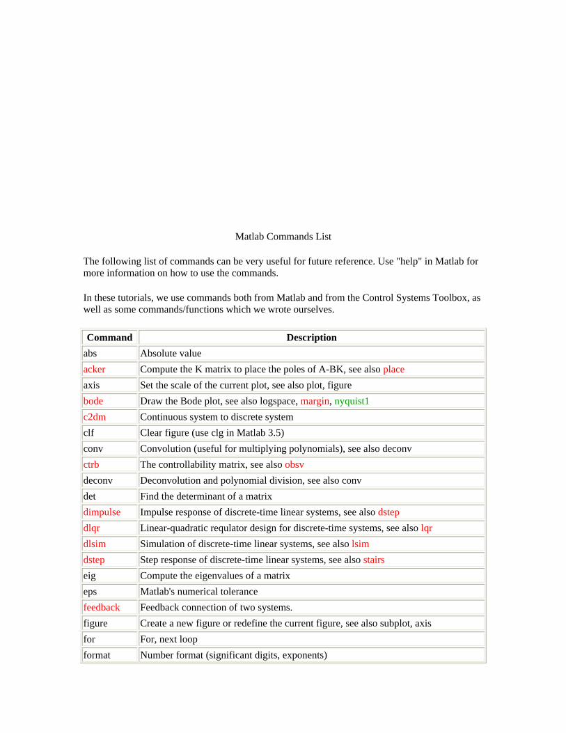
Matlab Com

following s can be very useful for future reference. Use "help" in Matlab for nforma

se tutor Control Systems Toolbox, as s some

nd ription

mands List

The list of commandmore i tion on how to use the commands.

In the ials, we use commands both from Matlab and from thewell a commands/functions which we wrote ourselves.

Comma Descabs Absolute value acker f A-BK, see also place Compute the K matrix to place the poles oaxis Set the scale of the current plot, see also plot, figure bode pace, margin, nyquist1 Draw the Bode plot, see also logsc2dm Continuous system to discrete system clf Clear figure (use clg in Matlab 3.5) conv Convolution (useful for multiplying polynomials), see also deconv ctrb The controllability matrix, see also obsv deconv n, see also conv Deconvolution and polynomial divisiodet Find the determinant of a matrix dimpulse Impulse response of discrete-time linear systems, see also dstep dlqr Linear-quadratic requlator design for discrete-time systems, see also lqr dlsim iscrete-time linear systems, see also lsim Simulation of ddstep Step response of discrete-time linear systems, see also stairs eig Compute the eigenvalues of a matrix eps Matlab's numerical tolerance feedback Feedback connection of two systems. figure new figure or redefine the current figure, see also subplot, axis Create afor For, next loop format exponents) Number format (significant digits,

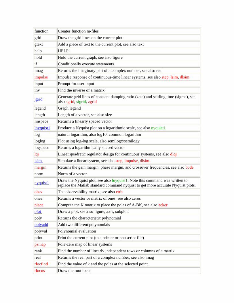
function Creates function m-files grid Draw the grid lines on the current plot gtext Add a piece of text to the current plot, see also text help HELP! hold Hold the current graph, see also figure if tements Conditionally execute staimag Returns the imaginary part of a complex number, see also real impulse Impulse response of continuous-time linear systems, see also step, lsim, dlsim input Prompt for user input inv Find the inverse of a matrix

jgrid Generate grid lines of constant damping ratio (zeta) and settling time (sigma), see also sgrid, sigrid, zgrid

legend Graph legend length Length of a vector, see also size linspace Returns a linearly spaced vector lnyquist1 Produce a Nyquist plot on a logarithmic scale, see also nyquist1 log natural logarithm, also log10: common logarithm loglog Plot using log-log scale, also semilogx/semilogy logspace Returns a logarithmically spaced vector lqr Linear quadratic regulator design for continuous systems, see also dlqr lsim Simulate a linear system, see also step, impulse, dlsim. margin see also bode Returns the gain margin, phase margin, and crossover frequencies,norm Norm of a vector

nyquist1 Draw the Nyquist plot, see also lnyquist1. Note this command was written to mand nyquist to get more accurate Nyquist plots. replace the Matlab standard com

obsv The observability matrix, see also ctrb ones Returns a vector or matrix of ones, see also zeros place Compute the K matrix to place the poles of A-BK, see also acker plot Draw a plot, see also figure, axis, subplot. poly Returns the characteristic polynomial polyadd Add two different polynomials polyval n Polynomial evaluatioprint Print the current plot (to a printer or postscript file) pzmap Pole-zero map of linear systems rank Find the number of linearly independent rows or columns of a matrix real eal part of a complex number, see also imag Returns the rrlocfind Find the value of k and the poles at the selected point rlocus Draw the root locus

roots ial Find the roots of a polynomrscale Find the scale factor for a full-state feedback system

set Set(gca,'Xtick',xticks,'Ytick',yticks) to control the number and spacing of tick marks on the axes

series Series interconnection of Linear time-independent systems

sgrid Generate grid lines of constant damping ratio (zeta) and natural frequency (Wn), see also jgrid, sigrid, zgrid

sigrid Generate grid lines of constant settling time (sigma), see also jgrid, sgrid, zgrid size Gives the dimension of a vector or matrix, see also length sqrt Square root ss Create state-space models or convert LTI model to state space, see also tf ss2tf State-space to transfer function representation, see also tf2ss ss2zp State-space to pole-zero representation, see also zp2ss stairs Stairstep plot for discreste response, see also dstep step Plot the step response, see also impulse, lsim, dlsim. subplot Divide the plot window up into pieces, see also plot, figure text Add a piece of text to the current plot, see also title, xlabel, ylabel, gtext tf Creation of transfer functions or conversion to transfer function, see also ss tf2ss Transfer function to state-space representation, see also ss2tf tf2zp Transfer function to Pole-zero representation, see also zp2tf title Add a title to the current plot

wbw Returns the bandwidth frequency given the damping ratio and the rise or settling time.

xlabel/ylabel , see also title, text, gtext Add a label to the horizontal/vertical axis of the current plot

zeros Returns a vector or matrix of zeros

zgrid Generates grid lines of constant damping ratio (zeta) and natural frequency (Wn), see also sgrid, jgrid, sigrid

zp2ss Pole-zero to state-space representation, see also ss2zp zp2tf Pole-zero to transfer function representation, see also tf2zp

Most of the following was provided by Mathworks Inc.

This case study demonstratedesign of a computer hard-d

s the ability to perform classical digital control design by going through the isk read/write head position controller.

Using Newton's law, a simple model for the read/write head is the differential equation

Deriving the Model

•

where is the inertia of the head assembly, is the viscous damping coefficient of the bearings, is the

return spring constant, is the motor torque constant, is the angular position of the head, and is the

Taking the Laplace transform, the transfer function from

input current.

to is

•

kg , Nm/rad, and Usin he values Nm/(rad/sec), g tNm , fo MATLAB prompt, type

4; K = 10; Ki = .05;

en = [J C K]; ,den)

/rad rm the transfer function description of this system. At the

• J = .01; C = 0.00um = Ki; • n

• d• H = tf(num

•

MA AB

ransfer function: • 0.05

---------- • 0.01 s^2 + 0.004 s + 10

The task here is to design a digital controller that provides accurate positioning of the read/write head. The desi is cause our plant will be equi ed er (with a zero-order hold) connected to its input, use c2d with the 'zoh' s

g period = 0.005 second

nsfer function: 5

-------------------- • z^2 - 1.973 z + 0.998

• Sampling time: 0.005

You can compare the Bode plots of the continuous and discretized models with

• bode(H,'-',Hd,'--')

TL responds with

• T

• -------------

•

Model Discretization

gn performed in the digital domain. First, discretize the continuous plant. Bepp with a digital-to-analog convert di cretization method. Type

• Ts = 0.005; % samplin• Hd = c2d(H,Ts,'zoh') • Tra• 6.233e-05 z + 6.229e-0• ---

•

•

•

•

To analyze the discrete system, plot its step response, type

• step(Hd)

•

•

The system oscillates quite a bit. This is probably due to very light damping. You can check this by computing the open-loop poles. Type

• % Open-loop poles of discrete model • damp(Hd) • Eigenvalue Magnitude Equiv. Damping Equiv. Freq. • • 9.87e-01 + 1.57e-01i 9.99e-01 6.32e-03

3.16e+01 • 9.87e-01 - 1.57e-01i 9.99e-01 6.32e-03

3.16e+01 •

The poles have very light equivalent damping and are near the unit circle. You need to design a compensator that increases the damping of these poles.

Right-Click Menus

The LTI Viewer provides a set of controls and options that you can access by right-clicking your mouse. Once you have imported a model into the LTI Viewer, the options you can select include

• Plot Type -- Change the plot type. Available types include step, impulse, Bode, Bode magnitude, Nichols, Nyquist, and singular values plots.

• Systems -- Select or clear any models that you included when you created the response plot.

• Characteristics -- Add information about the plot. The characteristics available change from plot to plot. For example, Bode plots have stability margins available, but step responses have rise time and steady-state values available.

• Grid -- Add grids to your plots. • Normalize -- Scale responses to fit the view (only available for time-domain plot types). • Full View -- Use automatic limits to make the entire curve visible. • Properties -- Open the Property Editor.

• You can use this editor to customize various attributes of your plot. See Customizing Plot Properties and Preferences online under "Customization" for a full description of the Property Editor.

Alternatively, you can open the Property Editor by double-clicking in an empty region of the response plot.

Displaying Response Characteristics on a Plot

For example, to see the rise time for the DC motor step response, right-click your mouse and select Rise Time under Characteristics, as this figure illustrates.

Figure 3-4: Using Right-Click Menus to Display the Rise Time for a Step Response

The rise time is defined as the amount of time it takes the step response to go from 10% to 90% of the steady-state value.

The LTI Viewer calculates and displays the rise time for the step response.

Figure 3-5: DC Motor Step Response with the Rise Time Displayed

To display the values of any plot characteristic marked on a plot, place your mouse on the blue dot that marks the characteristic. This opens a data marker with the relevant information displayed. To make the marker persistent, left-click on the blue dot.

For example, this figure shows the rise time value for the DC motor step response.

Figure 3-6: Using Your Mouse to Get the Rise Time Values

Note that you can left-click anywhere on a particular plot line to see the response values of that plot at that point. You must either place your cursor over the blue dot or left-click, however, if you want to see the rise time value.

For more information about data markers, see Data Markers.

Changing Plot Type

You can view other plots using the right-click menus in the LTI Viewer. For example, if you want to see the open loop Bode plots for the DC motor model, select Plot Type and then Bode from the right-click menu.

Figure 3-7: Changing the Step Response to a Bode Plot

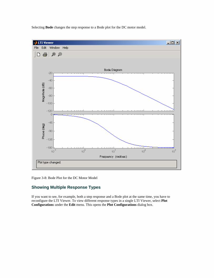
Selecting Bode changes the step response to a Bode plot for the DC motor model.

Figure 3-8: Bode Plot for the DC Motor Model

Showing Multiple Response Types

If you want to see, for example, both a step response and a Bode plot at the same time, you have to reconfigure the LTI Viewer. To view different response types in a single LTI Viewer, select Plot Configurations under the Edit menu. This opens the Plot Configurations dialog box.

Figure 3-9: Using the Plot Configurations Dialog Box to Reconfigure the LTI Viewer

You can select up to six plots in one viewer. Choose the Response type for each plot area from the right-hand side menus. There are nine available plot types:

• Step • Impulse • Bode (magnitude and phase) • Bode Magnitude (only) • Nyquist • Nichols • Sigma • Pole/Zero • I/O pole/zero

DC Motor

SISO Example: the DC MotorA simple model of a DC motor driving an inertial load shows the angular rate of the load, , as the output and applied voltage, , as the input. The ultimate goal of this example is to control the angular rate by varying the applied voltage. This picture shows a simple model of the DC motor. Figure 2-1: A Simple Model of a DC Motor Driving an Inertial Load In this model, the dynamics of the motor itself are idealized; for instance, the magnetic field is assumed to be constant. The resistance of the circuit is denoted by R and the self-inductance of the armature by L. If you are unfamiliar with the basics of DC motor modeling, consult any basic text on physical modeling. The important thing here is that with this simple model and basic laws of physics, it is possible to develop differential equations that describe the behavior of this electromechanical system. In this example, the relationships between electric potential and mechanical force are Faraday's law of induction and Ampère's law for the force on a conductor moving through a magnetic field. Mathematical DerivationThe torque seen at the shaft of the motor is proportional to the current i induced by the applied voltage, where Km, the armature constant, is related to physical properties of the motor, such as magnetic field strength, the number of turns of wire around the conductor coil, and so on. The back (induced) electromotive force, , is a voltage proportional to the angular rate seen at the shaft, where Kb, the emf constant, also depends on certain physical properties of the motor. The mechanical part of the motor equations is derived using Newton's law, which states that the inertial load J times the derivative of angular rate equals the sum of all the torques about the motor shaft. The result is this equation, where is a linear approximation for viscous friction. Finally, the electrical part of the motor equations can be described by or, solving for the applied voltage and substituting for the back emf, This sequence of equations leads to a set of two differential equations that describe the behavior of the motor, the first for the induced current, and the second for the resulting angular rate. State-Space Equations for the DC MotorGiven the two differential equations derived in the last section, you can now develop a state-space representation of the DC motor as a dynamical system. The current i and the angular rate are the two states of the system. The applied voltage, , is the input to the system, and the angular velocity is the output. Figure 2-2: State-Space Representation of the DC Motor Example

Getting Started Constructing SISO ModelsOnce you have a set of differential equations that describe your plant, you can construct SISO models using simple commands in the Control System Toolbox. The following sections discuss: Constructing a state-space model of the DC motor Converting between model representations Creating transfer function and zero/pole/gain models Constructing a State-Space Model of the DC MotorListed below are nominal values for the various parameters of a DC motor. R= 2.0 % Ohms

L= 0.5 % Henrys

Km = .015 % Torque constant

Kb = .015 % emf constant

Kf = 0.2 % Nms

J= 0.02 % kg.m^2/s^2

Given these values, you can construct the numerical state-space representation using the ss function. A = [-R/L -Kb/L; Km/J -Kf/J]

B = [1/L; 0];

C = [0 1];

D = [0];

sys_dc = ss(A,B,C,D)

This is the output of the last command. a =

x1 x2

x1 -4 -0.03

x2 0.75 -10

b =

u1

x1 2

x2 0

c =

x1 x2

y1 0 1

d =

u1

y1 0

Converting Between Model RepresentationsNow that you have a state-space representation of the DC motor, you can convert to other model representations, including transfer function (TF) and zero/pole/gain (ZPK) models. Transfer Function Representation. You can use tf to convert from the state-space representation to the transfer function. For example, use this code to convert to the transfer function representation of the DC motor. sys_tf = tf(sys_dc)

Transfer function:

1.5

------------------

s^2 + 14 s + 40.02

Zero/Pole/Gain Representation. Similarly, the zpk function converts from state-space or transfer function representations to the zero/pole/gain format. Use this code to convert from the state-space representation to the zero/pole/gain form for the DC motor. sys_zpk = zpk(sys_dc)

Zero/pole/gain:

1.5

-------------------

(s+4.004) (s+9.996)

Note The state-space representation is best suited for numerical computations. For highest accuracy, convert to state space prior to combining models and avoid the transfer function and zero/pole/gain representations, except for model specification and inspection. See Reliable Computations in the online Control System Toolbox documentation for more information on numerical issues. Constructing Transfer Function and Zero/Pole/Gain ModelsIn the DC motor example, the state-space approach produced a set of matrices that represents the model. If you choose a different approach, you can construct the corresponding models using tf, zpk, ss, or frd. sys = tf(num,den) % Transfer function

sys = zpk(z,p,k) % Zero/pole/gain

sys = ss(a,b,c,d) % State-space

sys = frd(response,frequencies) % Frequency response data

For example, if you want to create the transfer function of the DC motor directly, use these commands. s = tf('s');

sys_tf = 1.5/(s^2+14*s+40.02)

The Control System Toolbox builds this transfer function. Transfer function:

1.5

--------------------

s^2 + 14 s + 40.02

Alternatively, you can create the transfer function by specifying the numerator and denominator with this code. sys_tf = tf(1.5,[1 14 40.02])

Transfer function:

1.5

------------------

s^2 + 14 s + 40.02

To build the zero/pole/gain model, use this command. sys_zpk = zpk([],[-9.996 -4.004], 1.5)

This is the resulting zero/pole/gain representation. Zero/pole/gain:

1.5

-------------------

(s+9.996) (s+4.004)

Discrete Time SystemsThe Control Systems Toolbox provides full support for discrete time systems. You can create discrete systems in the same way that you create analog systems; the only difference is that you must specify a sample time period for any model you build. For example, sys_disc = tf(1, [1 1], .01); creates a SISO model in the transfer function format. Transfer function: 1 ----- z + 1 Sampling time: 0.01 Adding Time Delays to Discrete-Time ModelsYou can add time delays to discrete-time models by specifying an input or output time delay when building the model. The time delay must be a nonnegative integer that represents a multiple of the sampling time. For example, sys_delay = tf(1, [1 1], 0.01,'outputdelay',5); produces a system with an output delay of 0.05 second. Transfer function: 1 z^(-5) * ----- z + 1 Sampling time: 0.01 Adding Delays to Linear ModelsYou can add time delays to linear models by specifying an input or output delay when building a model. For example, to add an input delay to the DC motor, use this code. sys_tfdelay = tf(1.5, [1 14 40.02],'inputdelay',0.05) The Control System Toolbox constructs the DC motor transfer function, but adds a 0.05 second delay. Transfer function: 1.5 exp(-0.05*s) * ------------------ s^2 + 14 s + 40.02