MATLAB Basics 6 plotting

Anthony Rossiter

University of Sheffield

1

Slides by Anthony Rossiter

For a neat organisation of all videos and resources

http://controleducation.group.shef.ac.uk/indexwebbook.html

Introduction

1. The previous videos demonstrate how to use basic MATLAB functionality.

2. It is useful to next to consider how to form plots and graphs which look good and can be exported into reports and other formats.

3. A summary of the main plotting options is given here as more advanced users will easily be able to pursue further options.

Slides by Anthony Rossiter

2

List of common plotting options • Do your want multiple line plots on the same set of

axis? • Do you want multiple axis (subfigures) in the same

figure window? • Change colour, thickness and style of lines plots. • Adding labels to axis and a title and changing

fontsize. • Changing domain and range (equivalently ‘zoom in’). • Adding text, arrows, etc. • Saving a figure for further edit. • Exporting a figure as .eps, .jpg or other form for use

outside of MATLAB. • Etc.

Slides by Anthony Rossiter

3

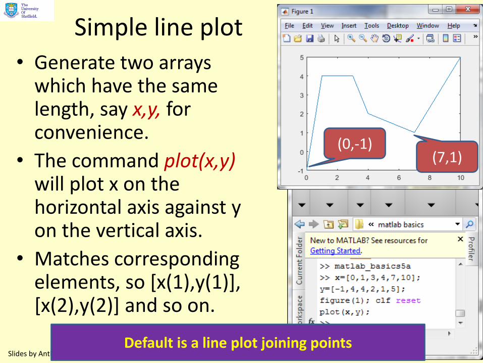
Simple line plot

• Generate two arrays which have the same length, say x,y, for convenience.

• The command plot(x,y) will plot x on the horizontal axis against y on the vertical axis.

• Matches corresponding elements, so [x(1),y(1)], [x(2),y(2)] and so on.

Slides by Anthony Rossiter

4

(0,-1) (7,1)

Default is a line plot joining points

Nominating a figure window

It is better to always say which figure window you wish to use or MATLAB will choose the one it thinks is active.

figure(1) - next plot statement will use figure 1.

figure(4) - next plot statement will use figure 4.

If you want the figure window to be clean, use ‘clf’ which is short for clean figure. This ensures you do not inherit any lines or other information from previous uses of that figure window.

Slides by Anthony Rossiter

5

Colours and markers

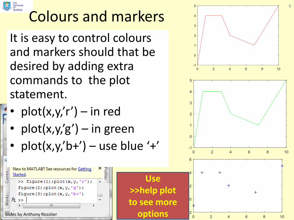
It is easy to control colours and markers should that be desired by adding extra commands to the plot statement.

• plot(x,y,’r’) – in red

• plot(x,y,’g’) – in green

• plot(x,y,’b+’) – use blue ‘+’

Slides by Anthony Rossiter

6

Use >>help plot to see more

options

Adding labels It is important that plots are presented nicely and

clearly.

• Use legend.m to match lines with colours.

• Use xlabel.m, ylabel.m to mark axis.

• Use title.m to give a figure title.

Experiment with putting in labels of your choice.

Use >> help title, and so on to get more detailed help on how to use these labels. We will give some illustrations.

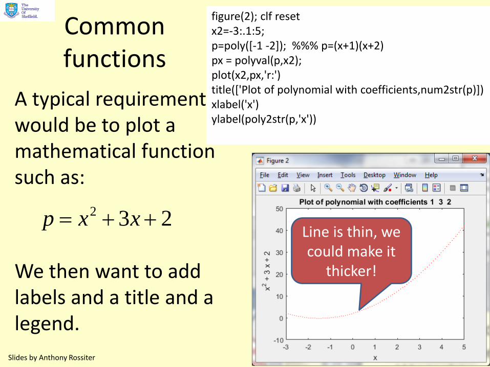
Common functions

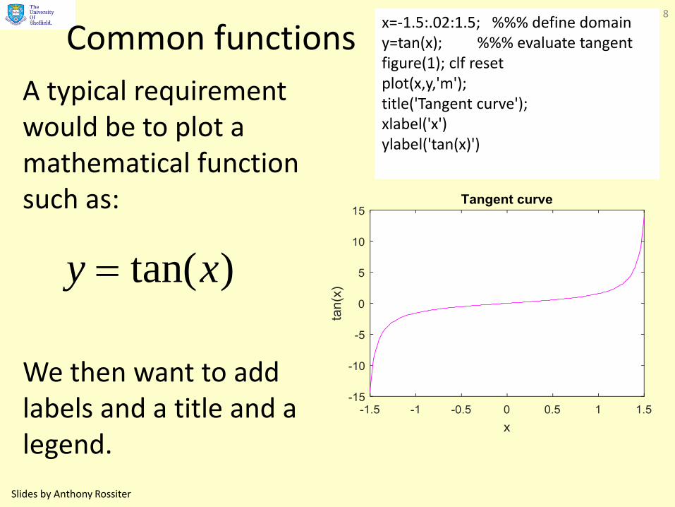
A typical requirement would be to plot a mathematical function such as:

We then want to add labels and a title and a legend.

Slides by Anthony Rossiter

8

)tan(xy

x=-1.5:.02:1.5; %%% define domain y=tan(x); %%% evaluate tangent figure(1); clf reset plot(x,y,'m'); title('Tangent curve'); xlabel('x') ylabel('tan(x)')

Common functions

A typical requirement would be to plot a mathematical function such as:

We then want to add labels and a title and a legend.

Slides by Anthony Rossiter

9

232 xxp

figure(2); clf reset x2=-3:.1:5; p=poly([-1 -2]); %%% p=(x+1)(x+2) px = polyval(p,x2); plot(x2,px,'r:') title(['Plot of polynomial with coefficients,num2str(p)]) xlabel('x') ylabel(poly2str(p,'x'))

Line is thin, we could make it

thicker!

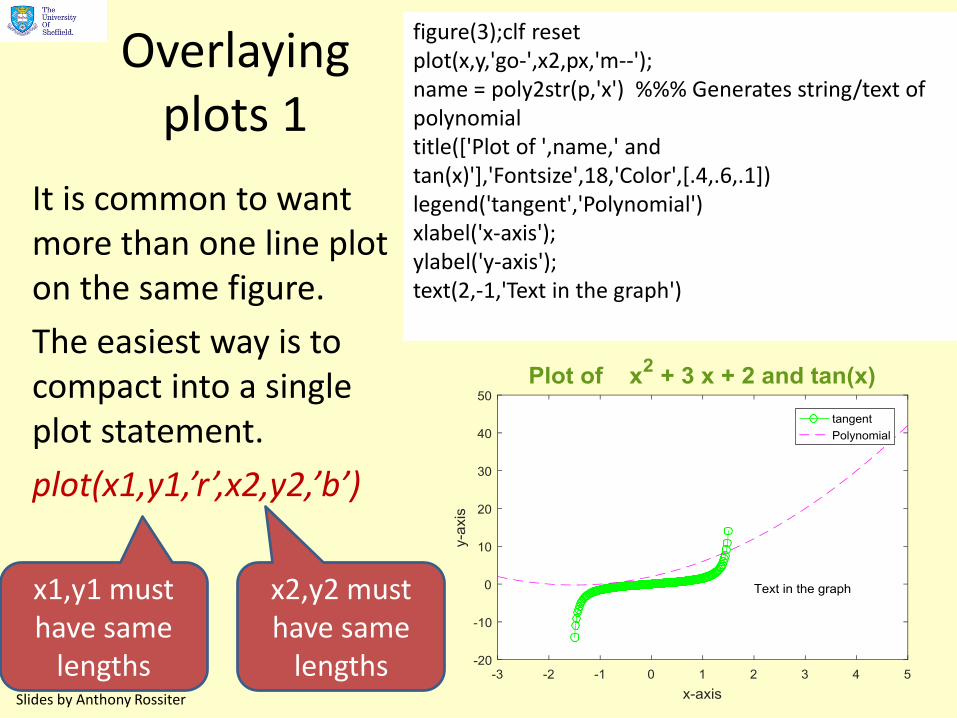
Overlaying plots 1

It is common to want more than one line plot on the same figure.

The easiest way is to compact into a single plot statement.

plot(x1,y1,’r’,x2,y2,’b’)

Slides by Anthony Rossiter

10 figure(3);clf reset plot(x,y,'go-',x2,px,'m--'); name = poly2str(p,'x') %%% Generates string/text of polynomial title(['Plot of ',name,' and tan(x)'],'Fontsize',18,'Color',[.4,.6,.1]) legend('tangent','Polynomial') xlabel('x-axis'); ylabel('y-axis'); text(2,-1,'Text in the graph')

x1,y1 must have same

lengths

x2,y2 must have same

lengths

Hold on and hold off

In many cases you may wish to overlay 4,5, 10 or more line plots.

• Putting these in a single command is clumsy, especially if you want different colours and markers.

• Also, you may generate a basic figure now and want to add a line plot to it later.

• The default with plot is to ‘clear existing line plots’, but you can override this with the ‘hold on’ command which instructs MATLAB to add the new line plot to the existing figure.

Slides by Anthony Rossiter

11

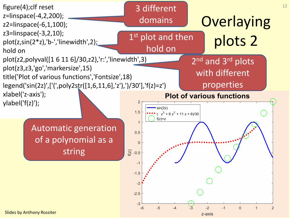
Overlaying plots 2

Slides by Anthony Rossiter

12 figure(4);clf reset z=linspace(-4,2,200); z2=linspace(-6,1,100); z3=linspace(-3,2,10); plot(z,sin(2*z),'b-','linewidth',2); hold on plot(z2,polyval([1 6 11 6]/30,z2),'r:','linewidth',3) plot(z3,z3,'go','markersize',15) title('Plot of various functions','Fontsize',18) legend('sin(2z)',['(',poly2str([1,6,11,6],'z'),')/30'],'f(z)=z') xlabel('z-axis'); ylabel('f(z)');

3 different domains

1st plot and then hold on

2nd and 3rd plots with different

properties

Automatic generation of a polynomial as a

string

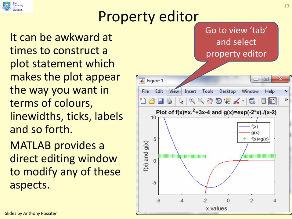
Property editor It can be awkward at times to construct a plot statement which makes the plot appear the way you want in terms of colours, linewidths, ticks, labels and so forth.

MATLAB provides a direct editing window to modify any of these aspects.

Slides by Anthony Rossiter

13

Go to view ‘tab’ and select

property editor

Slides by Anthony Rossiter

14

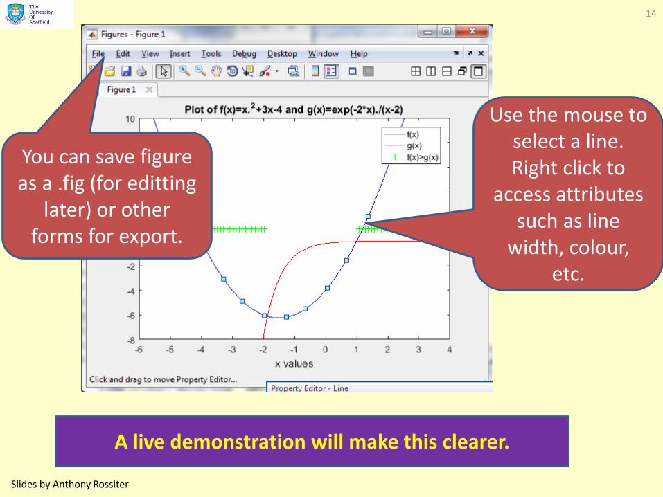
Use the mouse to select a line. Right click to

access attributes such as line

width, colour, etc.

A live demonstration will make this clearer.

You can save figure as a .fig (for editting

later) or other forms for export.

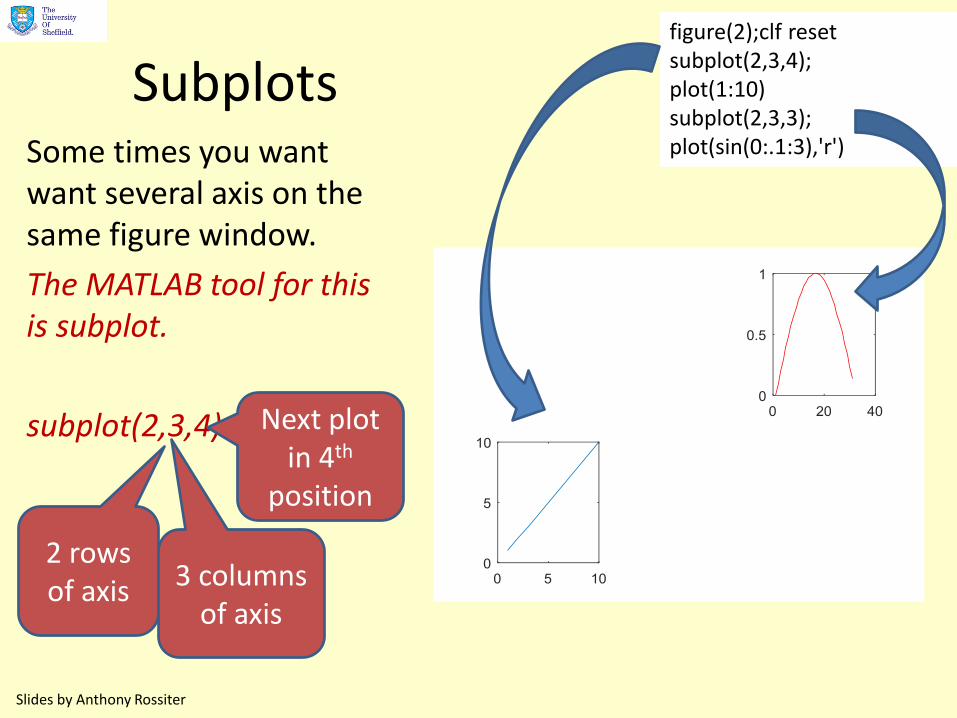
Subplots Some times you want want several axis on the same figure window.

The MATLAB tool for this is subplot.

subplot(2,3,4)

Slides by Anthony Rossiter

15 figure(2);clf reset subplot(2,3,4); plot(1:10) subplot(2,3,3); plot(sin(0:.1:3),'r')

2 rows of axis 3 columns

of axis

Next plot in 4th

position

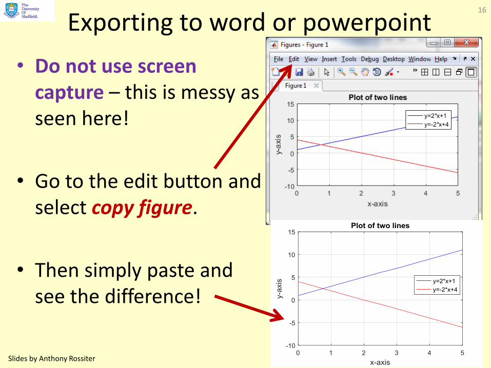
Exporting to word or powerpoint

• Do not use screen capture – this is messy as seen here!

• Go to the edit button and select copy figure.

• Then simply paste and see the difference!

Slides by Anthony Rossiter

16

LIVE DEMONSTRATIONS WITH MATLAB

Slides by Anthony Rossiter

17

Go through the following to see core plotting options and their use

matlab_basics6a.m

matlab_basics6b.m

Conclusions

Demonstrated the ease with which MATLAB can produce good quality plots for display.

1. Easy to control line colours, thickness and marker types.

2. Easy to overlay several line plots.

3. Easy to add labels, titles and legends.

4. Convenient editor for post processing.

5. Easy to save or export into any convenient format.

Slides by Anthony Rossiter

18

© 2016 University of Sheffield This work is licensed under the Creative Commons Attribution 2.0 UK: England & Wales Licence. To view a copy of this licence, visit http://creativecommons.org/licenses/by/2.0/uk/ or send a letter to: Creative Commons, 171 Second Street, Suite 300, San Francisco, California 94105, USA. It should be noted that some of the materials contained within this resource are subject to third party rights and any copyright notices must remain with these materials in the event of reuse or repurposing. If there are third party images within the resource please do not remove or alter any of the copyright notices or website details shown below the image. (Please list details of the third party rights contained within this work. If you include your institutions logo on the cover please include reference to the fact that it is a trade mark and all copyright in that image is reserved.)

Anthony Rossiter Department of Automatic Control and

Systems Engineering University of Sheffield www.shef.ac.uk/acse

For a neat organisation of all videos and resources

http://controleducation.group.shef.ac.uk/indexwebbook.html