CONTENTS

Preface xiAcknowledgments xv

Abbreviations xvii

P A R T I B A S E B A L LP A R T I B A S E B A L L

1. Baseball’s Pythagorean Theorem 3

2. Who Had a Better Year: Mike Trout or Kris Bryant? 12

3. Evaluating Hitters by Linear Weights 18

4. Evaluating Hitters by Monte Carlo Simulation 31

5. Evaluating Baseball Pitchers, Forecasting Future Pitcher Per for mance, and an Introduction to Statcast 44

6. Baseball Decision Making 60

7. Evaluating Fielders 73

8. Win Probability Added (WPA) 84

9. Wins Above Replacement (WAR) and Player Salaries 92

10. Park Factors 101

11. Streakiness in Sports 105

12. The Platoon Effect 124

13. Was Tony Perez a Great Clutch Hitter? 127

viii Contents

14. Pitch Count, Pitcher Effectiveness, and PITCHf/x Data 133

15. Would Ted Williams Hit .406 today? 139

16. Was Joe DiMaggio’s 56- Game Hitting Streak the Greatest Sports Rec ord of All Time? 142

17. Projecting Major League Per for mance 151

P A R T I I F O O T B A L LP A R T I I F O O T B A L L

18. What Makes NFL Teams Win? 159

19. Who’s Better: Brady or Rod gers? 164

20. Football States and Values 170

21. Football Decision Making 101 178

22. If Passing Is Better than Running, Why Don’t Teams Always Pass? 186

23. Should We Go for a One- Point or a Two- Point Conversion? 195

24. To Give Up the Ball Is Better than to Receive: The Case of College Football Overtime 207

25. Has the NFL Fi nally Gotten the OT Rules Right? 211

26. How Valuable Are NFL Draft Picks? 222

27. Player Tracking Data in the NFL 229

P A R T I I I B A S K E T B A L LP A R T I I I B A S K E T B A L L

28. Basketball Statistics 101: The Four Factor Model 249

29. Linear Weights for Evaluating NBA Players 259

30. Adjusted +/− Player Ratings 265

31. ESPN RPM and FiveThirtyEight RAPTOR Ratings 282

Contents ix

32. NBA Lineup Analy sis 289

33. Analyzing Team and Individual Matchups 296

34. NBA Salaries and the Value of a Draft Pick 303

35. Are NBA Officials Prejudiced? 307

36. Pick- n- Rolling to Win, the Death of Post Ups and Isos 313

37. SportVU, Second Spectrum, and the Spatial Basketball Data Revolution 321

38. In- Game Basketball Decision Making 341

P A R T I V O T H E R S P O R T SP A R T I V O T H E R S P O R T S

39. Soccer Analytics 355

40. Hockey Analytics 373

41. Volleyball Analytics 385

42. Golf Analytics 391

43. Analytics and Cyber Athletes: The Era of e- Sports 398

P A R T V S P O R T S G A M B L I N GP A R T V S P O R T S G A M B L I N G

44. Sports Gambling 101 409

45. Freakonomics Meets the Bookmaker 420

46. Rating Sports Teams 423

47. From Point Ratings to Probabilities 447

48. The NCAA Evaluation Tool (NET) 464

49. Optimal Money Management: The Kelley Growth Criterion 468

50. Calcuttas 474

x Contents

P A R T V I M E T H O D S A N D M I S C E L L A N E O U SP A R T V I M E T H O D S A N D M I S C E L L A N E O U S

51. How to Work with Data Sources: Collecting and Visualizing Data 479

52. Assessing Players with Limited Data: The Bayesian Approach 490

53. Finding Latent Patterns through Matrix Factorization 499

54. Network Analy sis in Sports 508

55. Elo Ratings 524

56. Comparing Players from Diff er ent Eras 531

57. Does Fatigue Make Cowards of Us All? The Case of NBA Back- to- Back Games and NFL Bye Weeks 538

58. The College Football Playoff 543

59. Quantifying Sports Collapses 551

60. Daily Fantasy Sports 559

Bibliography 569Index 579

C H A P T E R 1C H A P T E R 1

BASEBALL’S PYTHAGOREAN THEOREMThe more runs that a baseball team scores, the more games the team should win. Conversely, the fewer runs a team gives up, the more games the team should win. Bill James, prob ably the most celebrated advocate of applying mathe matics to analy sis of Major League Base-ball (often called sabermetrics), studied many years of Major League Baseball standings and found that the percentage of games won by a baseball team can be well approximated by the formula

runs scored2

runs scored2 + runs allowed2= Estimateof percentage

of games won. (1)

This formula has several desirable properties:

• Predicted win percentage is always between 0 and 1.• An increase in runs scored increases predicted win

percentage.• A decrease in runs allowed increases predicted win

percentage.

Consider a right triangle with a hypotenuse (the longest side) of length c and two other sides of length a and b. Recall from high school geometry that the Pythagorean Theorem states that a triangle is a right triangle if and only if a2 + b2 = c2 must hold. For example, a

4 Chapter 1

triangle with sides of lengths 3, 4, and 5 is a right triangle because 32 + 42 = 52. The fact that equation (1) adds up the squares of two numbers led Bill James to call the relationship described in (1) Base-ball’s Pythagorean Theorem.

Let’s define R = runs scoredruns allowed

as a team’s scoring ratio. If we

divide the numerator and denominator of (1) by (runs allowed)2, then the value of the fraction remains unchanged and we may re-write (1) as equation (1′).

R2

R2 +1= Estimate of percentage of gameswon (1′)

Figure 1-1 (see file Mathleticschapter1files.xlsx for all of this chap-ter’s analy sis) shows how well (1′) predicts teams’ winning percent-ages for Major League Baseball teams during the 2005–2016 sea-sons. For example, the 2016 Los Angeles Dodgers scored 725 runs

and gave up 638 runs. Their scoring ratio was R = 725638

=1.136. Their

predicted win percentage from Baseball’s Pythagorean Theorem

was 1.1362

1.1362 +1= .5636. The 2016 Dodgers actually won a fraction

91162

= .5618 of their games. Thus (1′) was off by 0.18% in predicting

the percentage of games won by the Dodgers in 2016.For each team define Error in Win Percentage Prediction to equal

Actual Winning Percentage minus Predicted Winning Percentage. For example, for the 2016 Atlanta Braves, Error = .42 − .41 = .01 (or 1.0%), and for the 2016 Colorado Rockies, Error = .46 − .49 = −.03 (or 3%). A positive error means that the team won more games than predicted while a negative error means the team won fewer games than predicted. Column J computes for each team the absolute value of the prediction error. Recall that absolute value of a number is simply the distance of the number from 0. That is, | 5 | = | −5 | = 5. In cell J1 we average the absolute prediction errors for each team to obtain a mea sure of how well our predicted win percentages fit the actual team winning percentages. The average of absolute forecasting

Baseball’s Pythagorean Theorem 5

errors is called the MAD (mean absolute deviation).1 We find that for our dataset the predicted winning percentages of the Pythagorean Theorem were off by an average of 2.17% per team.

Instead of blindly assuming win percentage can be approximated by using the square of the scoring ratio, perhaps we should try a formula to predict winning percentage, such as

Rexp

Rexp +1. (2)

If we vary exp in (2) we can make (2) better fit the actual dependence of winning percentage on the scoring ratio for diff er ent sports.

1. Why didn’t we just average the actual errors? Because averaging positive and negative errors would result in positive and negative errors canceling out. For ex-ample, if one team wins 5% more games than (1′) predicts and another team wins 5% less games than (1′) predicts, the average of the errors is 0 but the average of the absolute errors is 5%. Of course, in this simple situation estimating the average error as 5% is correct while estimating the average error as 0% is nonsensical.

123456789101112131415161718192021

A B C D E F G H I Jexp 2.000 MAD: 0.021

Year Team Wins Losses Runs Opp Runs Ratio Pred W–L% Act W–L% Error2016 ARI 69 93 752 890 0.845 0.42 0.43 0.0092016 ATL 68 93 649 779 0.833 0.41 0.42 0.0102016 BAL 89 73 744 715 1.041 0.52 0.55 0.0302016 BOS 93 69 878 694 1.265 0.62 0.57 0.0412016 CHC 103 58 808 556 1.453 0.68 0.64 0.0432016 CHW 78 84 686 715 0.959 0.48 0.48 0.0022016 CIN 68 94 716 854 0.838 0.41 0.42 0.0072016 CLE 94 67 777 676 1.149 0.57 0.58 0.0112016 COL 75 87 845 860 0.983 0.49 0.46 0.0282016 DET 86 75 750 721 1.040 0.52 0.53 0.0112016 HOU 84 78 724 701 1.033 0.52 0.52 0.0022016 KCR 81 81 675 712 0.948 0.47 0.50 0.0272016 LAA 74 88 717 727 0.986 0.49 0.46 0.0362016 LAD 91 71 725 638 1.136 0.56 0.56 0.0022016 MIA 79 82 655 682 0.960 0.48 0.49 0.0082016 MIL 73 89 671 733 0.915 0.46 0.45 0.0052016 MIN 59 103 722 889 0.812 0.40 0.36 0.0332016 NYM 87 75 671 617 1.088 0.54 0.54 0.0052016 NYY 84 78 680 702 0.969 0.48 0.52 0.034

F I G U R E 1 . 1F I G U R E 1 . 1 Baseball’s Pythagorean Theorem 2005–2016.

6 Chapter 1

For baseball, we will allow exp in (2) (exp is short for exponent) to vary between 1 and 3. Of course exp = 2 reduces to the Pythago-rean Theorem.

Figure 1-2 shows how the MAD changes as we vary exp between 1 and 3. This was done using the Data Table feature in Excel.2 We see that indeed exp = 1.8 yields the smallest MAD (1.99%). An exp value of 2 is almost as good (MAD of 2.05%), so for simplicity we will stick with Bill James’s view that exp = 2. Therefore exp = 2 (or 1.8) yields the best forecasts if we use an equation of form (2). Of course, there might be another equation that predicts winning percentage better than the Pythagorean Theorem from runs scored and allowed. The Pythago-

2. See Chapter 1 Appendix for an explanation of how we used Data Tables to de-termine how MAD changes as we vary exp between 1 and 3. Additional information available at https:// support . office . com / en - us / article / calculate - multiple - results - by - using - a - data - table - e95e2487 - 6ca6 - 4413 - ad12 - 77542a5ea50b.

F I G U R E 1 . 2F I G U R E 1 . 2 Dependence of Pythagorean Theorem Accuracy on Exponent.

567891011121314151617181920212223242526

N OMAD

0.0211.1 0.028122451.2 0.026179631.3 0.024415631.4 0.022892671.5 0.021602481.6 0.020690091.7 0.020142721.8 0.01992951.9 0.0201094

2 0.0205132.1 0.021144322.2 0.022087932.3 0.023287492.4 0.024734362.5 0.026402582.6 0.028238112.7 0.030193552.8 0.032285142.9 0.03447043

3 0.03670606

Baseball’s Pythagorean Theorem 7

rean Theorem is simple and intuitive, however, and does very well. After all, we are off in predicting team wins by an average of 162 * .0205, which is approximately three wins per team. Therefore, I see no reason to look for a more complicated (albeit slightly more accurate) model.

H O W W E L L D O E S T H E P Y T H A G O R E A N H O W W E L L D O E S T H E P Y T H A G O R E A N T H E O R E M F O R E C A S T ?T H E O R E M F O R E C A S T ?

To test the utility of the Pythagorean Theorem (or any prediction model) we should check how well it forecasts the future. We chose to compare the Pythagorean Theorem’s forecast for each Major League Baseball playoff series (2005–2016) against a prediction based just on games won. For each playoff series the Pythagorean method would predict the winner to be the team with the higher scoring ratio while the “games won” approach simply predicts the winner of a playoff series to be the team that won more games. We found that the Pythagorean approach correctly predicted 46 of 84 playoff series (54.8%) while the “games won” approach correctly predicted the winner of only 55% (44 out of 80) playoff series.3 The reader is prob-ably disappointed that even the Pythagorean method only correctly forecasts the outcome of under 54% of baseball playoff series. We believe that the regular season is a relatively poor predictor of the playoffs in baseball because a team’s regular season rec ord depends a lot on the per for mance of five starting pitchers. During the playoffs, teams only use three or four starting pitchers, so a lot of the regular season data (games involving the fourth and fifth starting pitchers) are not relevant for predicting the outcome of the playoffs.

For anecdotal evidence of how the Pythagorean Theorem fore-casts the future per for mance of a team better than a team’s win- loss rec ord, consider the case of the 2005 Washington Nationals. On July 4, 2005, the Nationals were in first place with a rec ord of 50–32. If we had extrapolated this win percentage, we would have predicted

3. In four playoff series the opposing teams had identical win- loss rec ords, so the “games won” approach could not make a prediction.

8 Chapter 1

a final rec ord of 99–63. On July 4, 2005, the Nationals’ scoring ratio was .991. On July 4, 2005, equation (1) would predict the Nationals to win around half (40) of the remaining 80 games and finish with a 90–72 rec ord. In real ity, the Nationals only won 31 of their remain-ing games and finished at 81–81!

I M P O R T A N C E O F P Y T H A G O R E A N T H E O R E MI M P O R T A N C E O F P Y T H A G O R E A N T H E O R E M

The Baseball Pythagorean Theorem is also impor tant because it al-lows us to determine how many extra wins (or losses) will result from a trade. As an example, suppose a team has scored 850 runs during a season and also given up 800 runs. Suppose we trade an  SS ( Joe) who “created”4 150 runs for a shortstop (Greg) who created 170 runs in the same number of plate appearances. This trade will cause the team (all other things being equal) to score

170 − 150 = 20 more runs. Before the trade, R = 850800

=1.0625, and we

would predict the team to have won 162 *1.06252

1+1.06252= 85.9 games.

After the trade, R = 870800

=1.0875, and we would predict the team to

have won 162 *1.08752

1+1.08752= 87.8 games. Therefore, we estimate the trade

makes our team 87.8 − 85.9 = 1.9 games better. In Chapter 9, we will see how the Pythagorean Theorem can be used to help determine fair salaries for Major League Baseball players.

F O O T B A L L A N D B A S K E T B A L L F O O T B A L L A N D B A S K E T B A L L “ P Y T H A G O R E A N T H E O R E M S ”“ P Y T H A G O R E A N T H E O R E M S ”

Does the Pythagorean Theorem hold for football and basketball? Daryl Morey, currently the General Man ag er for the Houston Rockets NBA team, has shown that for the NFL, equation (2) with

4. In Chapters 2–4 we will explain in detail how to determine how many runs a hitter creates.

Baseball’s Pythagorean Theorem 9

exp = 2.37 gives the most accurate predictions for winning percent-age, while for the NBA, equation (2) with exp = 13.91 gives the most accurate predictions for winning percentage. Figure 1-3 gives the predicted and actual winning percentages for the 2015 NFL, while Figure 1-4 gives the predicted and actual winning percentages for the 2015–2016 NBA. See the file Sportshw1.xls

For the 2008–2015 NFL seasons we found MAD was minimized by exp = 2.8. Exp = 2.8 yielded a MAD of 6.08%, while Morey’s exp = 2.37 yielded a MAD of 6.39%. For the NBA seasons 2008–2016 we found exp = 14.4 best fit actual winning percentages. The MAD for these seasons was 2.84% for exp = 14.4 and 2.87% for exp = 13.91. Since Morey’s values of exp are very close in accuracy to the values we found from recent seasons we will stick with Morey’s values of exp. See file Sportshw1.xls.

Assuming the errors in our forecasts follow a normal random variable (which turns out to be a reasonable assumption) we would

F I G U R E 1 . 3F I G U R E 1 . 3 Predicted NFL Winning Percentages: Exp = 2.37.

J K L M NMAD 0.051Act W-L% Error

0.813 0.0710.5 0.010 MAD

0.313 0.070 Exp 0.0511305580.5 0.032 1.5 0.087458019

0.938 0.179 1.6 0.0837863930.375 0.026 1.7 0.080410576

0.75 0.026 1.8 0.0772917280.188 0.072 1.9 0.074380834

0.25 0.075 2 0.0716988790.75 0.144 2.1 0.069282984

0.438 0.003 2.2 0.0670486720.625 0.0480.563 0.016 2.4 0.063455288

0.5 0.118 2.5 0.0621588110.313 0.085 2.6 0.0612796310.688 0.005 2.7 0.0608192710.375 0.006 2.8 0.0607587080.688 0.078 2.9 0.060941558

0.75 0.034 3 0.0613579210.438 0.028 3.1 0.0618918860.375 0.095 3.2 0.0626486370.625 0.004 3.3 0.0635949580.438 0.000 3.4 0.064745280.438 0.015 3.5 0.0659557420.625 0.036

2.3 0.065010818

123456789101112131415161718192021222324252627

A B C D E F G H I

Year2015201520152015201520152015201520152015201520152015201520152015201520152015201520152015201520152015

TeamArizona CardinalsAtlanta FalconsBaltimore RavensBuffalo BillsCarolina PanthersChicago BearsCincinnati BengalsCleveland BrownsDallas CowboysDenver BroncosDetroit LionsGreen Bay PackersHouston TexansIndianapolis ColtsJacksonville JaguarsKansas City ChiefsMiami DolphinsMinnesota VikingsNew England PatriotsNew Orleans SaintsNew York GiantsNew York JetsOakland RaidersPhiladelphia EaglesPittsburgh Steelers

Wins13

858

156

1234

127

10985

116

1112

76

1077

10

Losses38

1181

104

1312

49678

115

10549

106996

Ties0000000000000000000000000

PF PA Ratio489 313 1.56339 345 0.98328 401 0.82379 359 1.06500 308 1.62335 397 0.84419 279 1.50278 432 0.64275 374 0.74355 296 1.20358 400 0.90368 323 1.14339 313 1.08333 408 0.82376 448 0.84405 287 1.41310 389 0.80365 302 1.21465 315 1.48408 476 0.86420 442 0.95387 314 1.23359 399 0.90377 430 0.88423 319 1.33

Exp 2.370Pred W–L%

0.7420.4900.3830.5320.7590.4010.7240.2600.3250.6060.4350.5770.5470.3820.3980.6930.3690.6100.7160.4100.4700.6210.4380.4230.661

10 Chapter 1

expect around 95% of our NBA win forecasts to be accurate within 2.5 * MAD = 7.3%. Over 82 games this is about 6 games. So whenever the Pythagorean forecast for wins is off by more than six games, the Pythagorean prediction is an “outlier.” When we spot outliers we try and explain why they occurred. The 2006–2007 Boston Celtics had a scoring ratio of .966, and Pythagoras predicts the Celtics should have won 31 games. They won seven fewer games (24). During that season many people suggested the Celtics “tanked” games to improve their chance of having the #1 pick (Greg Oden and Kevin Durant went 1–2) in the draft lottery. The shortfall in the Celtics’ wins does not prove this conjecture, but the evidence is consistent with the Celtics win-ning substantially fewer games than chance would indicate.

F I G U R E 1 . 4F I G U R E 1 . 4 Predicted NBA Winning Percentages: Exp = 13.91.

123456789101112131415161718192021222324252627

A B C D E F G HExp 13.910

Year Team Wins Losses Points Opp Points Ratio Pred W-L%2015-16 Atlanta Hawks 48 34 8433 8137 1.04 0.6222015-16 Boston Celtics 48 34 8669 8406 1.03 0.6062015-16 Brooklyn Nets 21 61 8089 8692 0.93 0.2692015-16 Charlotte Hornets 48 34 8479 8256 1.03 0.5922015-16 Chicago Bulls 42 40 8335 8456 0.99 0.4502015-16 Cleveland Cavaliers 57 25 8555 8063 1.06 0.6952015-16 Dallas Mavericks 42 40 8388 8413 1 0.4902015-16 Denver Nuggets 33 49 8355 8609 0.97 0.3972015-16 Detroit Pistons 44 38 8361 8311 1.01 0.5212015-16 Golden State Warriors 73 9 9421 8539 1.1 0.7972015-16 Houston Rockets 41 41 8737 8721 1 0.5062015-16 Indiana Pacers 45 37 8377 8237 1.02 0.5582015-16 Los Angeles Clippers 53 29 8569 8218 1.04 0.6412015-16 Los Angeles Lakers 17 65 7982 8766 0.91 0.2142015-16 Memphis Grizzlies 42 40 8126 8310 0.98 0.4232015-16 Miami Heat 48 34 8204 8069 1.02 0.5572015-16 Milwaukee Bucks 33 49 8122 8465 0.96 0.3602015-16 Minnesota Timberwolves 29 53 8398 8688 0.97 0.3842015-16 New Orleans Pelicans 30 52 8423 8734 0.96 0.3772015-16 New York Knicks 32 50 8065 8289 0.97 0.4062015-16 Oklahoma City Thunder 55 27 9038 8441 1.07 0.7212015-16 Orlando Magic 35 47 8369 8502 0.98 0.4452015-16 Philadelphia 76ers 10 72 7988 8827 0.9 0.2002015-16 Phoenix Suns 23 59 8271 8817 0.94 0.2912015-16 Portland Trail Blazers 44 38 8622 8554 1.01 0.528

I J K L MMAD 0.0287Act W-L% Error

0.585 0.0370.585 0.0210.256 0.013 Exp 0.02870.585 0.007 12 0.03402860.512 0.062 12.2 0.03321350.695 6E-05 12.4 0.03242820.512 0.022 12.6 0.03171990.402 0.005 12.8 0.03104450.537 0.016 13 0.0304509

0.89 0.093 13.2 0.02989640.5 0.006 13.4 0.0294269

0.549 0.009 13.6 0.02904080.646 0.005 13.8 0.02875330.207 0.007 14 0.02859950.512 0.089 14.2 0.02849970.585 0.028 14.4 0.02844810.402 0.042 14.6 0.02847270.354 0.03 14.8 0.0285680.366 0.011 15 0.0287573

0.39 0.016 15.2 0.02896920.671 0.05 15.4 0.02926750.427 0.018 15.6 0.02961780.122 0.078 15.8 0.0300081

0.28 0.011 16 0.03045290.537 0.009

Baseball’s Pythagorean Theorem 11

C H A P T E R 1 A P P E N D I X : D A T A T A B L E SC H A P T E R 1 A P P E N D I X : D A T A T A B L E S

The Excel Data Table feature enables us to see how a formula changes as the values of one or two cells in a spreadsheet are modified. In this appendix we show how to use a one- way data table to determine how the accuracy of (2) for predicting team winning percentage de-pends on the value of exp. To illustrate let’s show how to use a one- way data table to determine how varying exp from 1 to 3 changes our average error in predicting an MLB’s team winning percentage (see Figure 1-2).

Step 1: We begin by entering the pos si ble values of exp (1, 1.1, . . . , 3) in the cell range N7:N26. To enter these values we simply enter 1 in N7 and 1.1 in N8 and select the cell range N7:N8. Now we drag the cross in the lower right- hand corner of N8 down to N26.

Step 2: In cell O6 we enter the formula we want to loop through and calculate for diff er ent values of exp by entering the formula = J1. Then we select the “ table range” N6:O26.

Step 3: Now we select Data Table from the What If section of the ribbon’s Data tab.

Step 4: We leave the row input cell portion of the dialog box blank but select cell G1 (which contains the value of exp) as the col-umn input cell. After selecting OK we see the results shown in Fig-ure 1-2. In effect, Excel has placed the values 1, 1.1, . . . , 3 into cell G1 and computed our MAD for each listed value of exp.

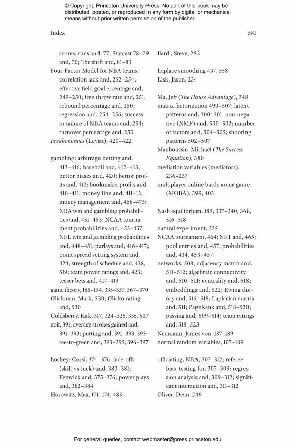
INDEX

Adler, Joseph, 65, 124, 127; Baseball Hacks, 65, 124, 127, 133

Albright, S. C., 120–121Annis, David, 345

back-to-back games, NBA teams and, 538–540

Baseball between the Numbers, 67Baseball Hacks (Adler), 54, 106Bayes theorem 490–494; average and,

293–295; conjugate distributions and, 494–495; evaluating kickers and, 494–496; Monty Hall and, 492–493; posterior distribution and, 493–494; prior and, 497–498

Bellman, Richard, 198Berk, Jonathan, 214Berri, David (Wages of Wins), 164, 259Berry, Scott, 534Big Data Bowl, 230Birnbaum, Phil, 183, 225Boswell, Thomas, 24Bowl Championship Series (BCS),

433; playoff alternatives and, 545; team rankings and, 433, 544–546

Braess paradox, 515

brainteaser, 150Brodie, Mark, 117; Every Shot Counts

and, 391Brook, Stacey (Wages of Wins), 164, 259Burke, Brian, 133–34; Bayesian evalu-

ation of QBs and, 498; deferring in NFL OT and, 217; value of football states and, 174

bye week, NFL teams, 540–542

Cabot, Vic, 172Calcutta auction, 474–476calibration curve (referred to also

as reliability or validation curve) 356–359, 389–390, 403, 459

Carter, Virgil, 172clustering 335–336, 340, 372; k-means

and, 513collapses, probabilities and, 551;

Mavericks and Raptors, 2019 and, 554; Mets, 1986 World Series and, 556–558; Patriots and Falcons, Super Bowl LI and, 552–554; Warriors and Cavaliers, 2016 NBA finals and, 551–552

conjugate distribution, 494

The letters t or f following a page number indicate a table or figure on that page.

580 Index

conversions: the chart and, 198–203; dynamic programming and, 198; one- point versus two- point, 195–197

convex hull, 239–240, 322–323Cook, Earnshaw (Percentage Baseball),

37

decision-making, baseball, 60, 70; base running and, 69–70; base steal-ing and, 67–69; bunting and, 67; expected value of random variables and, 63–65; experiments and ran-dom variables and, 63; possible states and, 61–62; runs per inning and, 72; tagging up from third base and, 71

decision-making, basketball, 341; corner three defense and, 335–339; end-game strategy and, 342–348; fouling with a three-point lead and, 344–348; lineup analysis and, 289–295; matchups and, 296–302; shooting three-point shot down two and, 342–344; two-person zero sum game theory (TPZSG), 337–338

decision-making, football, 178; accept-ing penalties and, 183; conversions and, 195–206; dynamic program-ming and, 198–203; field goal at-tempts and, 179–182; payoff matrix and, 186–193; possible states and, 170–174; punting and, 182–183; run-pass mix and, 184–185, 188–193; state values and, 175–177; two-person zero sum game theory (TPZSG) and, 186–193

Defense-Independent Component ERA (DICE), 53–55

Dewan, John 76; Fielding Bible and, 76–79

Dolphin, Andrew, 90, 134drafts: implied draft position value

curve, NFL and, 222–226; NBA ef-ficiency and, 305–306; NFL mock drafts and, 227; Winner’s Curse and, 227–228

eigenvalues and eigenvectors, 511–512, 514

e-sports 398–399; DOTA 2 hero adjusted +/—and, 401–403; DOTA 2 win probability and, 400–401; multiplayer online battle arena and, 399, 403; NBA2K league and, 404–405

Elo, 524; hyperparameters and, 525, 529–530; preseason NFL team rat-ings and, 526–528

Engelmann, Jeremias, 283, 287Excel: @RISK and, 37–38, 119; ad-

justed +/− ratings, 279–281; Analy-sis Toolpak Add-In, 29–30, 253; COUNTIFS, and SUMIFS functions in, 140; Data Table feature of, 6, 11, 42–43, 453, 456–457, 463; Monte Carlo simulation and, 32–34; Pois-son random variables and, 143–145, 443; regression tool and, 19, 29–30; Solver and, 270, 279–281, 414–415, 424, 427–428, 435–436, 442, 469, 532–533, 565–566; Trend Curve feature, 47, 59; VLOOKUP formula and, 426–427, 441, 454–455

fielders, evaluation of, 73; fielding per-centage and, 73–75; pitch framing and, 83; range factor and, 75–76; runs saved, wins and, 77–78;

Index 581

scores, runs and, 77; Statcast 78–79 and, 70; The shift and, 81–83

Four-Factor Model for NBA teams: correlation lack and, 252–254; effective field goal ercentage and, 249–250; free throw rate and, 251; rebound percentage and, 250; regression and, 254–256; success or failure of NBA teams and, 254; turnover percentage and, 250

Freakonomics (Levitt), 420–422

gambling: arbitrage betting and, 413–416; baseball and, 412–413; bettor biases and, 420; bettor prof-its and, 410; bookmaker profits and, 410–411; money line and, 411–12; money management and, 468–473; NBA win and gambling probabili-ties and, 451–453; NCAA tourna-ment probabilities and, 453–457; NFL win and gambling probabilities and, 448–451; parlays and, 416–417; point spread setting system and, 424; strength of schedule and, 428, 519; team power ratings and, 423; teaser bets and, 417–419

game theory, 186–194, 335–337, 367–370Glickman, Mark, 530; Glicko rating

and, 530Goldsberry, Kirk, 317, 324–325, 335, 507golf, 391; average strokes gained and,

391–393; putting and, 391–393, 395; tee-to-green and, 393–395, 396–397

hockey: Corsi, 374–376; face-offs (skill-vs-luck) and, 380–381; Fenwick and, 375–376; power plays and, 382–384

Horowitz, Max, 171, 174, 483

Ilardi, Steve, 283

Laplace smoothing 437, 558Lisk, Jason, 234

Ma, Jeff (The House Advantage), 348matrix factorization 499–507; latent

patterns and, 500–501; non-nega-tive (NMF) and, 500–502; number of factors and, 504–505; shooting patterns 502–507

Mauboussin, Michael (The Success Equation), 380

mediation variables (mediators), 236–237

multiplayer online battle arena game (MOBA), 399, 403

Nash equilibrium, 189, 337–340, 368, 516–518

natural experiment, 335NCAA tournament, 464; NET and, 465;

pool entries and, 457; probabilities and, 434, 453–457

networks, 508; adjacency matrix and, 511–512; algebraic connectivity and, 510–511; centrality and, 518; embeddings and, 522; Ewing the-ory and, 515–518; Laplacian matrix and, 511; PageRank and, 518–520; passing and, 509–514; team ratings and, 518–523

Neumann, James von, 187, 189normal random variables, 107–109

officiating, NBA, 307–312; referee bias, testing for, 307–309; regres-sion analysis and, 309–312; signifi-cant interaction and, 311–312

Oliver, Dean, 249

582 Index

On-Base Percentage (OBP), 26On-Base Plus Slugging (OPS), 26optimization: regression and, 19–21;

regularization and, 273–275ordinal logistic regression, 547–550overtime, NFL, 211–212; fair solution

and, 213–215; mathematical model of, 212–213

overtime college football, 207–210

p-values, 21–22page rank, 519Palmer, Pete, 24park factors, 101–104; range factor

and, 76payrolls: fair salary in MLB and,

98–99; NBA and, 303–304Pelton, Kevin, 285Percentage Baseball (Cook), 37Perez, Tony, 127–131pitchers, evaluation and forecasting

of: DICE and, 53–55; earned run average (ERA) and, 44–45; ERA as a predictive tool and, 47–49; MAD and, 51; saves and, 46

pitchers, pitch count and, 133–136platoon effect (splits), 67, 124–126players in different eras, 139–141;

aging and, 534; all-time greats and, 534–535; NBA player quality changes and, 531–534

players value: adjusted +/− ratings, NBA and, 267–275; ESPN RPM, NBA and, 283, 283t; luck ad-justed +/–, NBA and, 285; major league equivalents and, 151–153; Marcel projection and, 153–156; NBA draft efficiency and, 305–306; NBA efficiency rating and, 260–261, 261t; NFL draft picks and, 222–227;

plate appearances and, 82–83; PIMP, NBA and, 285; Player Ef-ficiency Rating (PER), NBA and, 261; pure +/− ratings, NBA and, 265–266; RAPTOR, NBA and 285, 283t; salaries and, 98–99, 303–305; Win Scores and Wins Produced 283t; Winner’s Curse and, 227–228; win scores and wins produced, NBA and, 262–264

player tracking data, 229, 321; convex hull and, 239–240, 322–323; corner 3s and, 329–340; defense and, 323–325; expected point value (DeepHoops) and, 325–329; NBA and, 321–340; NFL and, 229–246; offensive line and, 239–242; pass-ing (NFL) and, 230–239, 242–246

Player Win Averages, 84; baserunning and, 89; fielding ratings and, 88; Win Expectancy Finder and, 84–85

Pluto, Terry (Tall Tales), 265Poisson random variables, 143–145,

180, 358, 377–379, 442–445Pomeroy, Ken, 350predictions in sports, 57–58; Bradley-

Terry model and, 387–390; ERA using DICE and, 47, 54; gener-alized linear models and, 174, 180–181, 355–359; least squares team ratings and, 424–428; Marcel projection and, 153–156; NCAA tournament and, 453–457; net-work ratings and, 518–523; NFL playoffs and, 457–458; probability calibration (Platt scaling) and, 458–462; Pythagorean theorems and, 8–10, 385; ridge regression and, 273–275; soccer and, 442–446

Price, Joseph, 307, 312

Index 583

principal component analysis, 513–514probability matching, 370probability theory, 63; consecutive

no-hitters and, 148–150; DiMag-gio’s 56-game hitting streak and, 146–148; expected value and, 63–65; experiments and random variables and, 63; independent events and, 144; law of conditional expectation and, 65; law of rare events and, 143; NBA win and gam-bling probabilities and, 293–94; NCAA tournaments and, 294–96; NFL win and gambling probabili-ties and, 290–92; perfect games and, 144–145; pitching consecutive no hitters and, 148–150; sports col-lapses and, 551–558; team wins, bet covers and, 447–462.

Pythagorean Theorem: baseball and, 3–7; football and basketball and, 8–10; forecasting and, 7–8; mean absolute deviation (MAD) and, 5–6, 5f, 6f; runs, wins and, 78; Trout and, 40–41; volleyball and, 385

quarterbacks, rating of, 164–169; Burke’s regression and, 166–169, 166f, 167f

random variables, 63–65; expected value and, 64; independence and, 114, 144; normal distribution and, 107–109; Poisson and, 143–144; variances and, 291–292.

ranking teams: BCS and, 433–439; Elo and, 524–525; evaluating of-fenses and defenses and, 431–433; Glicko and, 530; home edge and, 290, 388, 424–425, 447, 524; mean absolute errors and, 428–431; mul-

tiplicative ratings and, 439–444; power ratings and, 424, 447; strength of schedule and, 428, 519; wins and losses and, 433–439

rare events, probability of, 143Reese, S., 534regressions, 18–20; Excel and, 29–30;

logistic and, 179–182, 216–218, 218t, 233–235, 233t, 234f, 235t, 241, 333, 334t, 356–357,357t; NBA officiating and, 309–312; Oliver’s Four Factors and, 255; ordinal logistic and, 547–550, 549t; p-values and, 21; quarterback ratings and, 166–169; ridge and , 273–275; scoring margins, NFL teams and, 159–162; Skellam, soccer and, 445

Romer, David, 172–174Rosen, Peter A., 207R-squared value (RSQ), 48–51; Excel

and, 56Runs Created formula, 13–15, 22, 152

sabermetrics, 3, 80, 380Sagarin, Jeff, 31, 37; clutch hitters and,

129; expected values (NFL) and, 172–173, 173t, NFL overtime, and 219–221; team ratings and, 431, 438–439, 447–448, 453–454, 539–542; WINVAL, 268–273

Schatz, Aaron, 58Schmidt, Martin (Wages of Wins), 164,

259Shandler, Ron, 58Silver, Nate (The Signal and the Noise),

497skill curves, 515–516slugging percentage (SLG), 12, 26–27,

27f, 152Smith, Ozzie, 75

584 Index

Sobel test (mediation variable), 237soccer: expected goals and, 355–358,

360–362; game theory and, 367–370; Markov chains and, 362–367; penalty kicks and, 367–370; player tracking data and, 371–372

Spurr, David, 45Stoll, Greg, Win Expectancy Finder

and, 84streakiness: baseball hitting and,

120–122; hot hand and, 107, 113–122; hot teams and, 122–123; hypothesis testing and, 112–113; normal random variables and, 107–109; random sequences and, 105–107; Wald Wolfowitz runs test (WWRT) and, 107, 111–112; z-scores and, 109–111

synergy: isolation and, 319–320; pick-and-roll and, 313–317; play type data, 313; post-ups and, 317–319

Tall Tales (Pluto), 265Tango, Tom: Marcel projection

system, 153–156; The Book and, 104, 134; weighted on-base average (wOBA) and, 93–94

Thaler, Richard, 222, 305Thomson, Bobby, 84, 91Tversky, A., 106–107, 113two-person zero sum game theory

(TPZSG), 186–194, 337–338, 367–370two proportion z-test, 383–384

Ulam, Stanislaw, 32

Vallone, R., 107, 113–114Ventura, Sam, 174, 373, 380, 483volleyball: Bradley-Terry model

and, 387–390; Pythagorean and, 385

Vollman, Rob (Stat Shot), 374

Wages of Wins (Berri, Schmidt, Brook), 164, 259

Wald Wolfowitz runs test (WWRT), 107, 111

Wilson, Rick L., 207–208Win Expectancy Finder, 84, 85f, 556,

557fWinner’s Curse: MLB free agents and,

99; NFL draft and, 227–228win probability: added baseball and,

84–88; DOTA 2 and, 399–404, 401t, 403f; in-game and, 553–554, 555–556; NFL and, 171, 174–175, 204–206, 218t; PageRank and, 521; Platt scaling and, 458–462; pulling the goalie and, 376–379; team rat-ings and, 447–458; volleyball and, 387–390, 390f

WINVAL ratings, 268; impact ratings and, 277–278; Khris Middleton contract and, 279; top 10 players and, 271f

Wolfers, Justin, 307, 312Woolner, Keith, 135

Yurko, Ron, 171, 174, 483

z-scores, 109–111, 113