MATHEMATICS OF COMPUTATIONVolume 74, Number 250, Pages 603–627S 0025-5718(04)01678-3Article electronically published on May 21, 2004

A FAST SWEEPING METHOD FOR EIKONAL EQUATIONS

HONGKAI ZHAO

Abstract. In this paper a fast sweeping method for computing the numer-ical solution of Eikonal equations on a rectangular grid is presented. Themethod is an iterative method which uses upwind difference for discretizationand uses Gauss-Seidel iterations with alternating sweeping ordering to solvethe discretized system. The crucial idea is that each sweeping ordering followsa family of characteristics of the corresponding Eikonal equation in a certaindirection simultaneously. The method has an optimal complexity of O(N) forN grid points and is extremely simple to implement in any number of dimen-sions. Monotonicity and stability properties of the fast sweeping algorithm areproven. Convergence and error estimates of the algorithm for computing thedistance function is studied in detail. It is shown that 2n Gauss-Seidel itera-tions is enough for the distance function in n dimensions. An estimation of thenumber of iterations for general Eikonal equations is also studied. Numericalexamples are used to verify the analysis.

1. Introduction

The Eikonal equation

(1.1) |∇u(x)| = f(x), x ∈ Rn,

with boundary condition, u(x) = φ(x), x ∈ Γ ⊂ Rn, has many applications inoptimal control, computer vision, geometric optics, path planing, etc. This nonlin-ear boundary value problem is a first order hyperbolic partial differential equation(PDE). Information propagates along characteristics from the boundary. Due tothe nonlinearity, characteristics may intersect like the formation of shocks in hyper-bolic conservation law. The solution is still continuous at these intersections butmay not be differentiable. The existence and uniqueness of the viscosity solutionare shown in [4].

There are two key ingredients for any numerical algorithm for the Eikonal equa-tion. The first key ingredient is the derivation of a consistent and accurate dis-cretization scheme, i.e., a numerical Hamiltonian. The numerical scheme has tofollow the causality of the partial differential equation and has to deal with non-differentiability at intersections of characteristics properly. Since the problem is

Received by the editor September 20, 2003.2000 Mathematics Subject Classification. Primary 65N06, 65N12, 65N15, 35L60.Key words and phrases. Eikonal equation, characteristics, Godunov scheme, upwind difference,

Gauss-Seidel iteration, Courant-Friedrichs-Lewy (CFL) condition.This work was partially supported by the Sloan Fundation, ONR grant N00014-02-1-0090 and

DARPA grant N00014-02-1-0603.

c©2004 American Mathematical Society

603

604 HONGKAI ZHAO

nonlinear, a large system of nonlinear equations has to be solved after the dis-cretization. Hence the second key ingredient is an efficient method for solving thelarge nonlinear system.

There are mainly two types of approaches for solving the Eikonal equation. Oneapproach is to transform it to a time dependent problem. For example, if we haveu(x) = 0, x ∈ Γ, then u(x) is the first arrival time at x for a wave front startingat Γ with a normal velocity that is equal to 1

f(x) . This can be solved by the levelset method. In the control framework, a semi-Lagrangian scheme is obtained forHamilton-Jacobi equations by discretizing in time the dynamic programming prin-ciple [9, 10]. However, many time steps may be needed for the convergence of thesolution in the entire domain due to finite speed of propagation and CFL condi-tion for time stability. The other approach is to treat the problem as a stationaryboundary value problem and to design an efficient numerical algorithm to solve thesystem of nonlinear equations after discretization. For example, the fast marchingmethod [19, 16, 11] is of this type. In the fast marching method, the update ofthe solution follows the causality in a sequential way; i.e., the solution is updatedone grid point by one grid point in the order that the solution is strictly increasing(decreasing). Hence an upwind difference scheme and a heapsort algorithm areneeded. The complexity is of order O(N log N) for N grid points, where the log Nfactor comes from the heapsort algorithm.

Here we present and analyze an iterative algorithm, called the fast sweepingmethod, for computing the numerical solution for the Eikonal equation on a rect-angular grid in any number of space dimensions. The fast sweeping method ismotivated by the work in [2] and was first used in [21] for computing the distancefunction. The main idea of the fast sweeping method is to use nonlinear upwinddifference and Gauss-Seidel iterations with alternating sweeping ordering. In con-trast to the fast marching method, the fast sweeping method follows the causalityalong characteristics in a parallel way; i.e., all characteristics are divided into a fi-nite number of groups according to their directions and each Gauss-Seidel iterationwith a specific sweeping ordering covers a group of characteristics simultaneously.The fast sweeping method is extremely simple to implement. The algorithm is op-timal in the sense that a finite number of iterations is needed. So the complexityof the algorithm is O(N) for a total of N grid points. The number of iterationsis independent of grid size. The accuracy is the same as any other method whichsolves the same system of discretized equations. The fast sweeping method hasbeen extended to more general Hamilton-Jacobi equations [18, 12]. Extensions tohigh order discretization will be studied in future reports.

The idea of alternating sweeping ordering was also used in Danielsson’s algo-rithm [6]. The algorithm computes the distance mapping, i.e., the relative (x, y)coordinate of a grid point to its closest point using an iterative procedure. Daniels-son’s algorithm is based on a strict dimension by dimension discrete formulationwhich in general does not follow the real characteristics of the distance function intwo and higher dimensions and hence results in low accuracy and twice as manyiterations compared to the fast sweeping method we present here. Danielsson’salgorithm does not work for distance functions to more general data sets such asthe distance to a curve or a surface. Neither does it extend to general Eikonalequations. Recently another discrete approach that uses the idea of fast sweepingmethod was proposed in [17]. It can compute the distance function more accurately

A FAST SWEEPING METHOD FOR EIKONAL EQUATIONS 605

but does not apply to general Eikonal equations either. Other related methods in-clude a dynamic programming approach and post sweeping idea in [15] and a groupmarching method in [13].

Here is the outline of the paper. In Section 2 we present the scheme and themotivation behind it. We then show a few monotonicity properties and a maximumchange principle for the fast sweeping algorithm in Section 3. In Section 4 we provethe convergence and error estimates for the distance function. We discuss the fastsweeping method for general Eikonal equations in Section 5. In Section 6 we presentnumerical results to verify our analysis and we show a few applications.

2. The fast sweeping algorithm and the motivation

We present the fast sweeping method for computing the viscosity solution u(x) ≥0 for the model problem

(2.1)|∇u(x)| = f(x), x ∈ Rn,u(x) = 0, x ∈ Γ ⊂ Rn,

where f(x) > 0. For simplicity the algorithm is presented in two dimensions. Theextension to higher dimensions is straightforward. We use xi,j to denote a gridpoint in the computational domain Ω, h to denote the grid size and uh

i,j to denotethe numerical solution at xi,j .

2.1. The fast sweeping algorithm.Discretization. We use the following Godunov upwind difference scheme [14]

to discretize the partial differential equation at interior grid points:

(2.2)[(uh

i,j − uhxmin)+]2 + [(uh

i,j − uhy min)+]2 = f2

i,jh2

i = 2, . . . , I − 1, j = 2, . . . , J − 1,

where uhx min = min(uh

i−1,j , uhi+1,j), uh

y min = min(uhi,j−1, u

hi,j+1) and

(x)+ =

x, x > 0,

0, x ≤ 0.

One sided difference is used at the boundary of the computational domain.For example, at a left boundary point x1,j , a one sided difference is usedin the x direction,

[(uh1,j − uh

2,j)+]2 + [(uh

1,j − uhy min)+]2 = f2

1,jh2.

Initialization. To enforce the boundary condition, u(x) = 0 for x ∈ Γ ⊂ Rn,assign exact values or interpolated values at grid points in or near Γ. Thesevalues are fixed in later calculations. Assign large positive values at allother grid points. These values will be updated later.

Gauss-Seidel iterationswith alternating sweeping orderings. At eachgrid xi,j whose value is not fixed during the initialization, compute thesolution, denoted by u, of (2.2) from the current values of its neighborsuh

i±1,j , uhi,j±1 and then update uh

i,j to be the smaller one between u and itscurrent value; i.e., unew

i,j = min(uoldi,j , u). We sweep the whole domain with

four alternating orderings repeatedly:

(1) i = 1 : I, j = 1 : J, (2) i = I : 1, j = 1 : J,(3) i = I : 1, j = J : 1, (4) i = 1 : I, j = J : 1.

606 HONGKAI ZHAO

The unique solution to the equation

(2.3) [(x − a)+]2 + [(x − b)+]2 = f2i,jh

2,

where a = uhx min, b = uh

y min, is

(2.4) x =

min(a, b) + fi,jh, |a − b| ≥ fi,jh,

a+b+√

2f2i,jh2−(a−b)2

2 , |a − b| < fi,jh.

In n dimensions the unique solution x to

(2.5) [(x − a1)+]2 + [(x − a2)+]2 + · · · + [(x − an)+]2 = f2i,jh

2

can be found in the following systematic way. First we order the ak’s in increasingorder. Without loss of generality, assume a1 ≤ a2 ≤ · · · ≤ an and define an+1 = ∞.There is an integer p, 1 ≤ p ≤ n, such that x is the unique solution that satisfies

(2.6) (x − a1)2 + (x − a2)2 + · · · + (x − ap)2 = f2i,jh

2 and ap < x ≤ ap+1;

i.e., x is the intersection of the straight line x = y, x, y ∈ Rp, with the spherecentered at a = (a1, a2, . . . , ap) of radius fi,jh in the first quadrant in Rp. We findx and p in the following recursive way. Start with p = 1. If x = a1 + fi,jh ≤ a2,then x = x. Otherwise find the unique solution x > a2 that satisfies

(x − a1)2 + (x − a2)2 = f2i,jh

2.

If x ≤ a3, then x = x. Otherwise repeat the procedure until we find p and x thatsatisfy (2.6).

Here are a few remarks about the algorithm:(1) The upwind difference scheme (2.2) is a special case of the general Godunov

numerical Hamiltonian proposed in [1]. The numerical Hamiltonian can bewritten as

Hh(Dx−ui,j, D

x+ui,j , D

y−ui,j, D

y+ui,j)

=√

max(Dx−ui,j)+, (Dx+ui,j)−2 + max(Dy

−ui,j)+, (Dy+ui,j)−2,

where

Dx−ui,j = ui,j−ui−1,j

h , Dx+ui,j = ui+1,j−ui,j

h ,

Dy−ui,j = ui,j−ui,j−1

h , Dy+ui,j = ui,j+1−ui,j

h ,

and (·)+ means taking the positive part and (·)− means taking the negativepart. Instead of using the upwind difference scheme (2.2), we can also use

[(uhi,j − uh

i−1,j)+]2 + [(uh

i,j − uhi+1,j)

+]2

+ [(uhi,j − uh

i,j−1)+]2 + [(uh

i,j − uhi,j+1)

+]2 = f2i,jh

2,

i = 2, . . . , I − 1, j = 2, . . . , J − 1,

(2.7)

which corresponds to the numerical Hamiltonian

Hh(Dx−ui,j , D

x+ui,j, D

y−ui,j , D

y+ui,j)

=√

[(Dx−ui,j)+]2 + [(Dx+ui,j)−]2 + [(Dy

−ui,j)+]2 + [(Dy+ui,j)−]2.

Both numerical Hamiltonians are monotone. The only difference betweenthese two formulations is at the intersections of characteristics. The second

A FAST SWEEPING METHOD FOR EIKONAL EQUATIONS 607

formulation may have larger truncation errors at those intersections as willbe explained in Section 4.

(2) In practice it may be desirable to restrict the computation to a neighbor-hood of the boundary Γ. For example, if we want to restrict the compu-tation in the neighborhood where the first arrival time is less than T , i.e.,xi,j : u(xi,j) < T , then we can use the following simple cutoff crite-rion: in the Gauss-Seidel iteration we update the solution at a grid pointxi,j only if at least one of its neighbors has a value smaller than T , i.e., ifmin(uh

x min, uhy min) < T .

(3) The large value assigned initially should be larger than the maximum pos-sible value of u(x) in the computation domain. For example, let fM =maxx∈Ω f(x) and let D be the diameter of the computational domain Ω.The initially assigned large value should be larger than FMD.

(4) In higher dimensions, the discretization (2.2) is easily extended dimensionby dimension and there are 2n different sweeping orderings in n dimensions.

(5) If we want to compute the viscosity solution u(x) ≤ 0 for (2.1), we modifythe discretization (2.2) to

(2.8)[(uh

i,j − uhxmax)−]2 + [(uh

i,j − uhy max)−]2 = f2

i,jh2,

i = 2, . . . , I − 1, j = 2, . . . , J − 1,

where uhx max = max(uh

i−1,j , uhi+1,j), uh

y max = max(uhi,j−1, u

hi,j+1) and

(x)− =

0, x > 0,

−x, x ≤ 0.

In the initialization, we assign small negative values at grid points whosevalues are to be updated. In the Gauss-Seidel iteration, we update the valueat a grid point only if the new value obtained by solving (2.8) is larger thanits old value.

2.2. The motivation. In the fast sweeping algorithm the upwind difference schemeused in the discretization enforces the causality; i.e., the solution at a grid pointis determined by its neighboring values that are smaller. The one sided differencescheme at the boundary enforces the propagation of information to be from insideto outside since the data set Γ is contained in the computational domain. If allgrid points can be ordered according to the causality along characteristics, one it-eration of the Gauss-Seidel iteration is enough for convergence. For example, theheapsort algorithm is used in the fast marching method to sort out this order everytime a grid point is updated. The key point behind Gauss-Seidel iterations withdifferent sweeping ordering is that each sweep will follow the causality of a groupof characteristics in certain directions simultaneously and all characteristics can bedivided into a finite number of such groups according to their directions. The valueat each grid point is always nonincreasing during the iterations due to the updatingrule. Whenever a grid point obtains the minimal value it can reach, the value isthe correct value and the value will not be changed in later iterations.

We use the distance function as an example to illustrate the motivation. Thedistance function d(x) to a set Γ satisfies the Eikonal equation

|∇d(x)| = 1, d(x) = 0, x ∈ Γ.

608 HONGKAI ZHAO

All characteristics of this equation are straight lines that radiate from the set Γ. Inone dimension, the upwind differencing at the interior grid point i is

(2.9) [(uhi − min(uh

i−1, uhi+1))

+]2 = h2, 2 ≤ i ≤ I − 1.

We use two Gauss-Seidel iterations with sweeping orderings, i = 1 : I and i = I : 1successively, to solve the above system. The update of the distance value at grid isimply becomes

unewi = min(min(ui−1, ui+1) + h, ui).

Figure 2.1 shows how one sweep from left to right followed by one more sweepfrom right to left is enough to finish the calculation of the distance function. Thisfollows because there are only two directions for the characteristics in one dimen-sion, left to right or vice versa. In another word, the distance value at any gridpoint can be computed from either its left neighbor or right neighbor by exactlydi = min(di−1, di+1) + h. The first sweep will cover those characteristics that gofrom left to right; i.e., those grid points whose values are determined by theirleft neighbors are computed correctly. Similarly, in the second sweep all those gridpoints whose values are determined by their right neighbors are computed correctly.Since we only update the current value if the newly computed value is smaller, thosevalues that have been calculated correctly in the first sweep have achieved their min-imal possible values and will not be changed in the second sweep. Convergence intwo sweeps is true for arbitrary Eikonal equations in one dimension. In the specialcase of the distance function, it is easy to see that the fast sweeping method findsthe exact distance function in two sweeps.

In higher dimensions characteristics have infinitely many directions which cannotbe followed exactly by the Cartesian grid lines. Here are two important questions forthe fast sweeping algorithm: (1) How many Gauss-Seidel iterations are needed? (2)What is the error estimate? The most important observation is that all directions ofcharacteristics can be classified into a finite number of groups for distance functions.For example, in two dimensions all directions of characteristics can be classified intofour groups, up-right, up-left, down-left and down-right. Information propagatesalong characteristics in the above four groups of directions. The four differentorderings of the Gauss-Seidel iterations and the upwind differencing are meant tocover the four groups of characteristics, respectively. Figure 2.2(a) illustrates whythe fast sweeping method converges after four sweeps with different orderings forthe distance function to a single point. The solution uh

i,j at each grid point in thefirst quadrant depends on the solution at uh

i−1,j and uhi,j−1 which have already been

computed and can be recursively traced all the way back to the data point in thefirst sweep. So we get the correct values for all grid points in the first quadrantplus the points on the positive x and y axes after the first sweep. For the samereason, after the second sweep the grid points in the second quadrant and on the

(a) the computed distance function af-ter the first left to right Gauss-Seidelsweeping

(b) the computed distance function af-ter the second right to left Gauss-Seidel sweeping

Figure 2.1. The fast sweeping algorithm in one dimension.

A FAST SWEEPING METHOD FOR EIKONAL EQUATIONS 609

i=1:I, j=1:J

i=1:I, j=J:1

i=I:1, j=1:J

i=I:1, j=J:1

i

j

(a) the fast sweeping algorithm for asingle data point

i

j

i=1:I, j=1:J

i=1:I, j=1,J

i=1:i, j=J:1

i=1:i, j=J:1

i=I:1, j=1:J

i=I:1, j=1:J

i=I:1, j=J:1

i=I:1, j=J:1

(b) the fast sweeping algorithm for acircle

Figure 2.2. The fast sweeping algorithm in two dimensions.

negative x axis get the correct values. Moreover, since those grid points in thefirst quadrant and on the positive x and y axes already have their minimal valuesand satisfy the discretized equations, these values will not change in the secondsweep. Similarly, after the third sweep those grid points in the third quadrantand on the negative y axis get the correct values and the computed correct valuesin the first and second quadrants are maintained. After four sweeps we get thecorrect values for all grid points that satisfy the system of equations (2.2). Figure2.2(b) demonstrates another case which computes the distance function to a circlein two dimensions using the fast sweeping algorithm. Again, each grid point getsits correct value in one of the four sweeps.

In the case of one data point, the distance function is smooth except at thedata point. For a more general data set, interactions of characteristics at theirintersections can cause more than 2n sweeps for the iteration to converge in ndimensions. It is impossible to track the exact number of sweeps for the highlynonlinear discretized system in general. However, we will show that in n dimensions,after 2n sweeps the fast sweeping method can compute a numerical solution to thedistance function that is as accurate as the numerical solution after the iterationconverges. This means 2n sweeps is good enough in practice for computing thedistance function to an arbitrary data set. For general Eikonal equations, thecharacteristics are curves instead of straight lines. So more than one sweep maybe needed to cover one characteristic curve. We will see that given a fixed domainand the right-hand side f(x), the number of sweeps needed is still finite and isindependent of grid size.

3. Basic properties of the fast sweeping algorithm

Here we prove a few basic monotonicity properties and a maximum change prin-ciple for the fast sweeping algorithm. The following simple fact for the solution ofequation (2.5) provides the monotonicity and maximum change principle for thefast sweeping algorithm.

610 HONGKAI ZHAO

Lemma 3.1. Let x be the solution to equation (2.5). We have

(3.1) 1 ≥ ∂x

∂a1≥ ∂x

∂a2≥ · · · ≥ ∂x

∂an≥ 0

and

(3.2)∂x

∂a1+

∂x

∂a2+ · · · + ∂x

∂an= 1.

Proof. Differentiating equation (2.5) with respect to ak, we get

∂x

∂ak=

(x − ak)+∑nm=1(x − am)+

.

As a direct consequence of the lemma, we have

Proposition 3.2. In the Gauss-Seidel iteration for the fast sweeping method, themaximum change of uh at any grid point is less than or equal to the maximumchange of uh at its neighboring points.

Lemma 3.3. The fast sweeping algorithm is monotone in the initial data.

Proof. This is a direct consequence from Lemma 3.1; i.e., the monotonicity propertyof the solution to (2.5). If uh(xi,j) ≤ vh(xi,j) at all grid points initially, thenuh(xi,j) ≤ vh(xi,j) at all grid points after any number of Gauss-Seidel iterations.

Lemma 3.4. The solution of the fast sweeping algorithm is nonincreasing witheach Gauss-Seidel iteration.

Proof. This is exactly because of the way we update the solution in the Gauss-Seideliterations described in the third step of the algorithm.

The following corollary shows the stability property for the fast sweeping method.We present it in two dimensions but it is true in general.

Corollary 3.5. Let u(k) and v(k) be two numerical solutions at the k-th iterationof the fast sweeping algorithm. Let ‖ · ‖∞ be the maximum norm. We have

(1) ‖u(k) − v(k)‖∞ ≤ ‖u(k−1) − v(k−1)‖∞,(2) 0 ≤ maxi,ju(k)

i,j − u(k+1)i,j ≤ maxi,ju(k−1)

i,j − u(k)i,j .

Proof. Let us assume that the first update at the k-th iteration is at point xi,j ,u

(k)i,j = minu(k−1)

i,j , u, where u solves (2.2) with neighboring values u(k−1)i−1,j , u

(k−1)i+1,j ,

u(k−1)i,j−1 , u

(k−1)i,j+1 . The same is true for v

(k)i,j . From the maximum change principle, we

have|u(k)

i,j − v(k)i,j | ≤ ‖u(k−1) − v(k−1)‖∞.

For an update at any other grid point later in the iteration, the neighboring valuesused for the update are either from the previous iteration or from an earlier updatein the current iteration, both of which satisfy the above bound. By induction, weprove (1).

The second statement is a simple consequence of the monotonicity of the fastsweeping method and the previous statement by setting v(k) = u(k−1).

A FAST SWEEPING METHOD FOR EIKONAL EQUATIONS 611

Remark. The second statement provides an effective stopping criterion for sweeping.Before correct information from the boundary Γ has reached all grid points, ‖u(k)−u(k−1)‖∞ is of O(1). When ‖u(k) − u(k−1)‖∞ is O(h), the information has reachedall points and we can stop the sweeping in practice. Although the iteration has notconverged yet, the numerical solution is already as accurate as the converged oneas we will see from the numerical examples. The iterative solution will change lessand less in later iterations and converges to the solution of the discretized system.

Theorem 3.6. The iterative solution by the fast sweeping algorithm convergesmonotonically to the solution of the discretized system.

Proof. Denote the numerical solution after the k-th sweep by u(k)i,j . Since u

(k)i,j

is bounded below by 0 and is nonincreasing with Gauss-Seidel iterations, u(k)i,j is

convergent for all i, j. After each sweep, for each i, j we have

[(u(k)i,j − u

(k)xmin)+]2 + [(u(k)

i,j − u(k)y min)+]2 − f2

i,jh2 ≥ 0,

because any later update of neighbors of u(k)i,j in the same sweep is nonincreasing.

Moreover, it is easy to see that after u(k)i,j is updated, the function

F (u(k)i−1,j , u

(k)i+1,j , u

(k)i,j−1, u

(k)i,j+1) = [(u(k)

i,j − u(k)x min)+]2 + [(u(k)

i,j − u(k)y min)+]2 − f2

i,jh2

is Lipschitz continuous in all variables and the Lipschitz constant is bounded by

2 max(u(k)i,j − u

(k)i−1,j)

+, (u(k)i,j − u

(k)i+1,j)

+, (u(k)i,j − u

(k)i,j−1)

+, (u(k)i,j − u

(k)i,j+1)

+.Since u

(k)i,j is monotonically convergent for every i, j, we can have an upper bound

C > 0 for the Lipschitz constant. Let δ(k) = maxi,j(u(k−1)i,j − u

(k)i,j ) be the maxi-

mum change at all grid points during the k-th sweep. From Corollary 3.5 and theconvergence of u

(k)i,j , δ(k) goes monotonically to zero. After the k-th iteration, we

have0 ≤ [(u(k)

i,j − u(k)x min)+]2 + [(u(k)

i,j − u(k)y min)+]2 − f2

i,jh2 ≤ Cδ(k).

So u(k)i,j converges to the solution to (2.2).

4. Convergence and error estimate for the distance function

Although it is shown that the fast sweeping algorithm is convergent by Theorem3.6, the main issue for the efficiency of the fast sweeping method is the number ofiterations needed and the error estimate. In this section we prove a few concreteresults for the distance function. Since the fast sweeping algorithm is highly nonlin-ear, the proof can only be based on the monotonicity properties and the maximumchange principle proved in Section 3. Some of the proofs will be stated in twodimensions for simplicity. We use the following notations: Γ denotes the data setto which we want to compute the distance function, uh(x, Γ) denotes the numer-ical solution using the fast sweeping method, d(x, Γ) denotes the exact distancefunction, h is the grid size, and n is the spatial dimension.

Theorem 4.1. For a single data point Γ = x0, the numerical solution, uh(x, x0),of the fast sweeping method converges in 2n sweeps in Rn and satisfies

d(x, x0) ≤ uh(x, x0) ≤ d(x, x0) + O(|h log h|),where d(x, x0) is the distance function to x0.

612 HONGKAI ZHAO

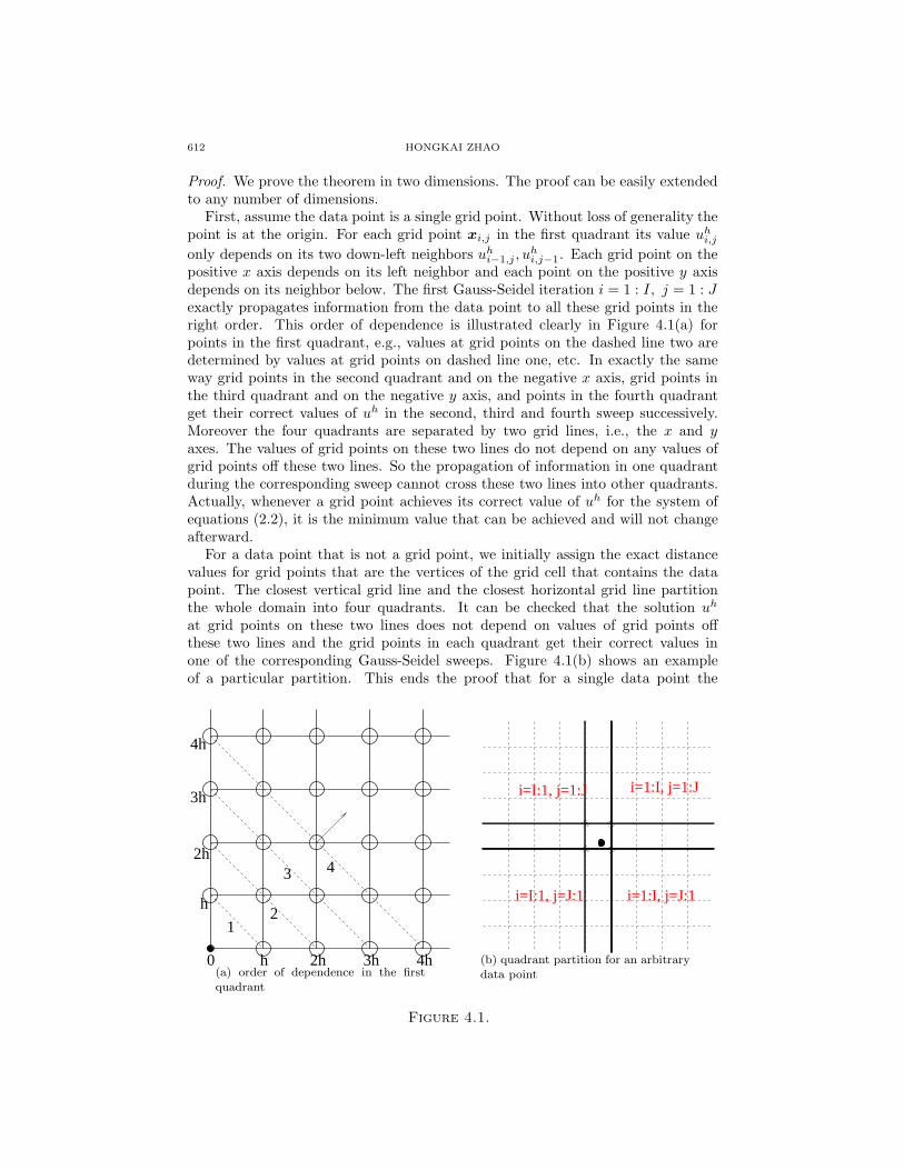
Proof. We prove the theorem in two dimensions. The proof can be easily extendedto any number of dimensions.

First, assume the data point is a single grid point. Without loss of generality thepoint is at the origin. For each grid point xi,j in the first quadrant its value uh

i,j

only depends on its two down-left neighbors uhi−1,j , u

hi,j−1. Each grid point on the

positive x axis depends on its left neighbor and each point on the positive y axisdepends on its neighbor below. The first Gauss-Seidel iteration i = 1 : I, j = 1 : Jexactly propagates information from the data point to all these grid points in theright order. This order of dependence is illustrated clearly in Figure 4.1(a) forpoints in the first quadrant, e.g., values at grid points on the dashed line two aredetermined by values at grid points on dashed line one, etc. In exactly the sameway grid points in the second quadrant and on the negative x axis, grid points inthe third quadrant and on the negative y axis, and points in the fourth quadrantget their correct values of uh in the second, third and fourth sweep successively.Moreover the four quadrants are separated by two grid lines, i.e., the x and yaxes. The values of grid points on these two lines do not depend on any values ofgrid points off these two lines. So the propagation of information in one quadrantduring the corresponding sweep cannot cross these two lines into other quadrants.Actually, whenever a grid point achieves its correct value of uh for the system ofequations (2.2), it is the minimum value that can be achieved and will not changeafterward.

For a data point that is not a grid point, we initially assign the exact distancevalues for grid points that are the vertices of the grid cell that contains the datapoint. The closest vertical grid line and the closest horizontal grid line partitionthe whole domain into four quadrants. It can be checked that the solution uh

at grid points on these two lines does not depend on values of grid points offthese two lines and the grid points in each quadrant get their correct values inone of the corresponding Gauss-Seidel sweeps. Figure 4.1(b) shows an exampleof a particular partition. This ends the proof that for a single data point the

0 h 2h 3h 4h

h

2h

3h

4h

12

3 4

(a) order of dependence in the firstquadrant

i=1:I, j=1:Ji=I:1, j=1:J

i=I:1, j=J:1 i=1:I, j=J:1

(b) quadrant partition for an arbitrarydata point

Figure 4.1.

A FAST SWEEPING METHOD FOR EIKONAL EQUATIONS 613

fast sweeping algorithm converges in four Gauss-Seidel iterations with alternatingsweeping ordering in two dimensions.

Now we show the error estimate for grid points in the first quadrant. The proofis exactly the same for all other quadrants. Again we first assume the data pointis a grid point. The exact distance function d(x) satisfies the Eikonal equation|∇d(x)| = 1 everywhere except at the data point. Using Taylor expansion at gridpoint xi,j , we have

di,j − di−1,j = h(dx)i,j − h2

2 dxx(ξi,j),

di,j − di,j−1 = h(dy)i,j − h2

2 dyy(ηi,j),(4.1)

where ξi,j and ηi,j are two intermediate points on the line segments connecting xi,j ,xi−1,j and connecting xi,j , xi,j−1, respectively. At x = (x, y),

(4.2)dx(x, y) = x√

x2+y2> 0, 0 < dxx(x, y) = y2

(x2+y2)3/2 ≤ 1√x2+y2

,

dy(x, y) = y√x2+y2

> 0, 0 < dyy(x, y) = x2

(x2+y2)3/2 ≤ 1√x2+y2

.

So the distance function satisfies the following equation at xi,j :

(4.3) [di,j − (di−1,j − h2

2dxx(ξi,j))]2 + [di,j − (di,j−1 − h2

2dyy(ηi,j))]2 = h2.

Since the solution of the quadratic equation (2.3) depends monotonically on (a, b),we have d(x, x0) ≤ uh(x, x0). Using the explicit expression (4.2) for the derivativesand the maximum change principle, the local truncation error satisfies

(4.4) eT (xi,j) ≤ h2

2max(dxx(xi−1,j), dyy(xi,j−1)) ≤ h2

2 min(d(xi−1,j), d(xi,j−1)).

The global error estimate comes from the fact the accumulation of truncation errorsis in the same direction of information propagation as is shown in Figure 4.1(a);i.e., grid points on line i + j = k depend only on grid points on line i + j ≤ k − 1.Define ek = maxi+j=k(uh

i,j − di,j). Using the simple fact that

d(xi,j) = h√

i2 + j2,(i + j)2

2≤ i2 + j2 ≤ (i + j)2,

and the maximum change principle, we have

uhi,j − di,j ≤ max(uh

i−1,j − di−1,j +h2

2dxx(xi−1,j),

uhi,j−1 − di,j−1 +

h2

2dxx(xi,j−1))

≤ ek−1 +h2

2 min(d(xi−1,j), d(xi,j−1))≤ ek−1 +

h√2(k − 1)

.

So the maximum error that can be accumulated at xi,j for k = i + j is

(4.5) ek ≤ e1 +h√2

i+j−1∑k=1

1k≤ e1 +

h√2(1 + ln(i + j − 1)) = O(h log(

1h

)).

Here e1 is the maximum error for grid points on the line i + j = 1, which is 0 ifthe data point is a grid point. The proof and estimate are exactly the same in ndimensions.

614 HONGKAI ZHAO

If the data point x0 is not a grid point, all the error estimates are the sameexcept that e1 = O(h), which yields the same result.

Remark. The error estimate is sharp since there is no cancellation of local truncationerrors and the accumulation of truncation errors for grid points xi,i on the diagonalis exactly of O(h log( 1

h )).

When there is more than one data point, the situation becomes more complicatedbecause there are interactions among data points. Characteristics from differentdata points intersect and the distance function is not differentiable at equal distancepoints. For the exact distance function to a data set composed of discrete points,i.e., Γ = xmM

m=1, the interaction is simply the minimum rule, i.e.,

d(x, Γ) = min[d(x, x1), d(x, x2), . . . , d(x, xM )].

Let uh(x, xi) be the numerical solution to the distance function to a single pointxi by the fast sweeping method and define

(4.6) uh(x, Γ) = min[uh(x, x1), uh(x, x2), . . . , uh(x, xM )].

From our previous results for a single point we have

d(x, Γ) ≤ uh(x, Γ) ≤ d(x, Γ) + O(|h log h|)after four sweeps.

Lemma 4.2. For an arbitrary set of discrete points Γ = xmMm=1, uh(x, Γ) ≤

uh(x, Γ).

Proof. For any fixed x there is an i, 1 ≤ i ≤ M , such that

uh(x, Γ) = min[uh(x, x1), uh(x, x2), . . . , uh(x, xM )] = uh(x, xi).

After the initialization step, uh(x, Γ) ≤ uh(x, xi), 1 ≤ i ≤ M . From the mono-tonicity in initial data for the fast sweeping algorithm, stated in Lemma 3.3, wehave

uh(x, Γ) ≤ uh(x, xi) = uh(x, Γ)

after any number of sweeps.

Let uh(x, Γ) be the solution to the system of discretized equations, e.g., (2.2) intwo dimensions.

Theorem 4.3. For an arbitrary set of discrete points Γ = xmMm=1, the numerical

solution uh(x, Γ) by the fast sweeping method after 2n sweeps, satisfies

uh(x, Γ) ≤ uh(x, Γ) ≤ d(x, Γ) + O(|h log h|).Proof. The solution to the system of discretized equations, uh(x, Γ), can be viewedas the solution by the fast sweeping algorithm after the iteration converges asis shown in Theorem 3.6. Since the solution of the fast sweeping algorithm isnonincreasing with Gauss-Seidel iterations, we have uh(x, Γ) ≥ uh(x, Γ) after anynumber of sweeps. So after 2n sweeps, the numerical solution uh(x, Γ) producedby the fast sweeping algorithm satisfies

uh(x, Γ) ≤ uh(x, Γ) ≤ uh(x, Γ) = d(x, Γ) + O(h log1h

).

A FAST SWEEPING METHOD FOR EIKONAL EQUATIONS 615

Since the upwind difference is of first order accuracy, |uh(x, Γ) − d(x, Γ)| is atmost O(h). The general results for Hamilton Jacobi equations, e.g., [5, 14, 3, 7],show that the numerical solution from a consistent and monotone scheme convergesto the viscosity solution with the order of h

12 . The upper bound in the above

theorem is sharp as is shown in Theorem 4.1. If the error estimate, |uh(x, Γ) −d(x, Γ)|, is also O(|h log h|) or worse, the theorem says that for the distance function,the iterative solution after 2n sweeps is as accurate as uh(x, Γ). Any other methodthat solves the same discretized system of equations has the same accuracy too.

However, we do not have d(x, Γ) ≤ uh(x, Γ) for a general data set Γ due to theinteractions among data points. Figure 4.2 shows an example of two data points.At those circled grid points the characteristics from both data points meet. Thedistance function follows either one of the characteristics. For example at grid point(1, 1) the distance function satisfies

[(d1,1 − d1,2)+]2 = h2 or [(d1,1 − d2,1)+]2 = h2

and d1,1 = 2h. However in our upwind scheme, the numerical solution uh uses bothcharacteristics and satisfies

[(uh1,1 − uh

1,2)+]2 + [(uh

1,1 − uh2,1)

+]2 = h2,

which gives uh1,1 = (1 + 1√

2)h < d1,1. We can view this as the information propaga-

tion speed is numerically doubled. However, since the upwind scheme uses at mosttwo characteristics from ux min in the x-direction and from uy min in the y-directionin two dimensions, we show that this is actually the worst truncation error that canoccur at a grid point due to the interactions of data points, i.e. when characteristicsintersect orthogonally and align with both axes. For instance in two dimensions,without loss of generality suppose uh

i,j ≥ uhi,j−1 ≥ uh

i−1,j and

(uhi,j − uh

i−1,j)2 + (uh

i,j − uhi,j−1)

2 = h2.

Then (uhi,j − uh

i−1,j)2 ≥ h2/2 and the equality holds when uh

i,j−1 = uhi−1,j. On the

other hand the distance function satisfies (di,j−di−1,j)2 ≤ h2 and the equality holdswhen the x axis is a characteristic. In n dimensions, the characteristics can be usedat most n times when they intersect at one grid point. So the worst local truncation

error due to the interactions of characteristics is√

1 − 1nh. For the modified version

of the fast sweeping algorithm (2.7), the truncation errors at equal distance pointscan be twice as much.

To get a clearer picture of the convergence of the iteration and error estimate for ageneral data set, we have to study the interactions among data points more carefully.We can partition all grid points into the Voronoi cell of each data point. TheVoronoi diagram is according to the the numerical solution uh(x, x1), uh(x, x2), . . . ,uh(x, xM ); i.e., a grid point x is in the Voronoi cell of xm if

uh(x, xm) = min[uh(x, x1), uh(x, x2), . . . , uh(x, xM )].

If a grid point and all its neighboring grid points belong to the same Voronoi cell, wecall it an interior point. Otherwise we call it a boundary point. The interaction ofdifferent data points occurs only at boundary points. Figure 4.3(a) shows a typicalVoronoi cell for a data point xm. For cell boundary points (those circled points),uh(x, Γ) may pick up information from more than one data point.

616 HONGKAI ZHAO

x

x

1

2(1,1) (1,2) (1,3)

(2,1) (2,2) (2,3)

(3,1) (3,2) (3,3)

The numerical solution for two datapoints 1,2

Figure 4.2.

xm

Voronoi cellxi,j x

x

(a) error at the cell boundary and itspropagation

domain of dependence

Voronoi cell

x m(b) domain of dependence of a gridpoint

Figure 4.3.

To get the lower bound for the numerical solution after 2n sweeps, we useuh(x, Γ) = min[uh(x, x1), uh(x, x2), . . . , uh(x, xM )] as the initial data and startthe fast sweeping iteration. Due to the monotonicity in initial data we get a solu-tion that provides a lower bound for the numerical solution for which we use thestandard initialization step. uh(x, Γ) already satisfies the discretized equations atinterior points of each Voronoi cell. After we start the fast sweeping algorithm, thedecrease of the values at interior points of each Voronoi cell is caused by the inter-actions at Voronoi cell boundaries. Moreover, if we start with uh(xi,j , Γ), it is easyto show |uh(xi,j , Γ)−uh(xi±1,j±1, Γ)| ≤ h from the system of discretized equationsat each grid point and the definition of Voronoi cells. Hence from the maximumchange principle Proposition 3.2, we can imagine that the maximum decrease ofvalues at all grid points due to the interactions at the Voronoi cell boundary isof order h. But unlike the case for the real distance function where informationpropagates only along characteristics and all characteristics flow into the Voronoicell boundary, in the finite difference scheme a grid point may have a larger domainof dependence as is illustrated in Figure 4.3(b). So interactions at Voronoi cellboundaries may propagate into the cell. This may also cause more than 2n sweeps

A FAST SWEEPING METHOD FOR EIKONAL EQUATIONS 617

for convergence in n dimensions. Example 1 in Section 6 shows that even for twodata points in two dimensions, more than four sweeps are needed for the iterationto converge.

Now we consider computing the distance function to an arbitrary set. For ex-ample, instead of discrete points, Γ is a smooth curve or surface.

Theorem 4.4. If the distance function in the neighborhood of an arbitrary data setΓ in Rn is given initially, let uh(x, Γ) be the numerical solution by the fast sweepingmethod after 2n sweeps. We have

uh(x, Γ) ≤ uh(x, Γ) ≤ d(x, Γ) + O(h log1h

),

where uh(x, Γ) is the solution to the discretized system (2.2).

Proof. Let Γ be the set of grid points that encloses the set Γ; i.e., Γ contains verticesof all those grid cells that intersect with Γ. We have

(4.7) |d(x, Γ) − d(x, Γ)| = O(h),

since for any y ∈ Γ, ∃yi,j ∈ Γ such that |yi,j − y| = O(h) and vice versa.By the monotonicity in initial data, uh(x, Γ) ≥ uh(x, Γ) after any number of

sweeps, since initially uh(x, Γ) starts with distance to Γ for x ∈ Γ while uh(x, Γ) = 0for x ∈ Γ. However, the initial difference between uh(x, Γ) and uh(x, Γ) is O(h).By the contraction property from Corollary 3.5, we have

(4.8) uh(x, Γ) − uh(x, Γ) = O(h), ∀x,

after any number of sweeps. We apply Theorem 4.3 to uh(x, Γ) and combine itwith (4.7) and (4.8) to finish the proof.

Actually for an arbitrary data set, which can be discrete points and/or continuousmanifolds, we only need approximate distance values at grid points near the dataset within first order accuracy, since the upwind finite difference scheme is at mostof first order.

5. General Eikonal equations

For the general Eikonal equation (2.1), the characteristics are curves startingfrom the boundary. The key issue is the maximum number of sweeps needed to coverinformation propagation along a single characteristic curve. This number, which isanalogous to the condition number for elliptic equations, determines the numberof iterations needed for the fast sweeping algorithm. For a single characteristiccurve starting at a point x0 ∈ Γ, we divide it into the least number of pieces suchthat the tangent directions in each piece belong to the same quadrant. Informationpropagation along each piece can be covered by one of the sweepings orderingsuccessively. So the number of sweeps needed to cover the whole characteristiccurve is proportional to the number of pieces or turns. Figure 5.1 shows an examplein 2D. The characteristic curve starting from x0 ∈ Γ can be divided into five pieces.The tangent directions in each piece belong to the same quadrant. If we order oneround of four alternating sweeps as in Section 2, the first and the second piecesare covered by the first and fourth sweeps in the first round, respectively, the thirdpiece is covered by the third sweep in the second round, the fourth piece is coveredby the second sweep in the third round and the fifth piece is covered by the firstsweep in the fourth round.

618 HONGKAI ZHAO

x 0

1 2

3

4

5

Ω

Γ

Figure 5.1. Division of a characteristic curve for a generalEikonal equation.

One quantity that can characterize how sharp the tangent of a curve can turn iscurvature. The following lemma shows a bound on the curvature of any character-istic curve.

Lemma 5.1. The maximum curvature for any characteristic curve of equation

(2.1) is bounded by maxx∈Ω

∣∣∣∣∇f(x)f(x)

∣∣∣∣.Proof. Denote H(q, x) = |q| − f(x), where q = ∇u. The characteristic equation is

x = ∇qH = ∇u

f(x) ,

q = −∇xH = ∇f(x),u = ∇u · x = f(x).

The information propagates along the characteristics from smaller u to larger u.Since |x| = 1, the curvature along a characteristic is

x =∇u

f(x)− ∇u

f2(x)∇f · x

=∇f(x)f(x)

−(∇f(x)

f(x)· ∇u

|∇u|) ∇u

|∇u|=

∇f(x)f(x)

− Pn∇f(x)f(x)

,

where Pn is the projection on the normal direction n =∇u

|∇u| . So |x| ≤∣∣∣∣∇f(x)

f(x)

∣∣∣∣.

A FAST SWEEPING METHOD FOR EIKONAL EQUATIONS 619

So for general Eikonal equations the number of iterations for the fast sweepingmethod depends on the right-hand side f(x) and the size and dimension of the com-putational domain only. The computed numerical solution has the same accuracyas the solution by any other method that uses the same discretization.

If the boundary Γ and f(x) are smooth and f(x) > 0, then Γ is a noncharac-teristic boundary and there is a neighborhood of Γ in which characteristics do notcross each other and the solution u(x) is smooth (see [8]). Let this neighborhoodbe ΩΓ. We have

Theorem 5.2. The numerical solution uhi,j to the discretized system (2.2) is of

first order in ΩΓ; i.e., |uhi,j − u(xi,j)| = O(h), xi,j ∈ ΩΓ.

Proof. Without loss of generality, suppose the numerical solution to (2.2) satisfiesthe equation

(uhi,j − uh

i−1,j)2 + (uh

i,j − uhi,j−1)

2 = f2i,jh

2

at a grid point xi,j , while the true solution u(x) satisfies

[ui,j − (ui−1,j − h2

2uxx(ξi,j))]2 + [ui,j − (ui,j−1 − h2

2uyy(ηi,j))]2 = f2

i,jh2

at xi,j , where ξi,j and ηi,j are two intermediate points on the line segments con-necting xi,j , xi−1,j and connecting xi,j , xi,j−1, respectively. Since uxx, uyy arebounded, from the maximum change property, Lemma 3.1, we can deduce that thelocal truncation error is O(h2). The propagation and accumulation of truncationerrors following the causality along characteristics in a finite domain is at mostO(h).

This error estimate breaks down when the solution has singularities. Since thecharacteristics do intersect for general Eikonal equations, we cannot use this ar-gument after characteristics intersect. We quote the general error estimate resultsfor monotone schemes for Hamilton-Jacobi equations [5, 14, 3, 7]. The error is oforder O(h1/2). In general, there are two scenarios for the solution to have singular-ities. In the first scenario Γ is smooth but characteristics intersect and shocks areformed. The solution is continuous but not differentiable at shocks. The numericalsolution can be only first order accurate at shocks. However, characteristics andinformation flow into shocks for the true solution. Numerically we also observe thaterrors made at shocks do not propagate away from shocks and hence high orderschemes can achieve high order accuracy in smooth regions. In the second scenarioΓ has singularities such as corners and kinks. Hence the solution also has singular-ities at Γ. The distance function to a single point is such an example. Again onlyfirst order accuracy can be achieved near the boundary for any numerical scheme.Since characteristics and information flow out of the boundary, errors made nearthe boundary will propagate out to the computational domain. So the global errorwill be at most of first order no matter what scheme is used. The only solution isto use a finer grid near singularities at the boundary.

6. Numerical results

In this section we will use numerical examples to test the fast sweeping algo-rithm and to verify the analysis in previous sections. We can compute the distancefunction only in a narrow neighborhood of the data set as is described in Section 2if needed, which saves an order of magnitude of computational cost.

620 HONGKAI ZHAO

For computing the distance function to a set of discrete points, we use the fol-lowing procedure for the initialization step. First initialize the distance value of allgrid points to be a large value, which should be larger than the maximum possiblevalues for our later computed distance value uh in the domain. Then go througheach data point and update the distance values of its neighboring grid points. Forexample, for each data point we find the grid cell that contains it and then computethe exact distance value of vertices of the grid cell to the data point. We replacethe current values of these vertices whenever distance to this data point providesa smaller value. Of course we can include more neighboring grid points for whichthe exact distance values are computed. In our calculations, distance values arecomputed at grid points that are within two grid cells of the data set in the ini-tialization step except for the first example. After going through all data points,we have computed exact distance values at those grid points in a neighborhood ofthe data set. All other grid points remain to have a large value. This procedure isof complexity O(M) for M data points. In general we can find the global distancefunction to any data set as long as the distance values on grid points neighboringthe set are provided or computed initially.

Example 1. This example shows the interaction of two data points on a simplegrid in two dimensions. Five iterations are needed for the fast sweeping algorithm toconverge. However, changes after four iterations are O(h) no matter what size thegrid is as we have tested. In Figure 6.1 we show the results after each iteration ona 7× 7 grid. The two data points are grid points at (2, 6), (5, 2). For this example,we scale the grid size to be 1. Initially, as is shown in Table 6.1(a), we assign a largeenough number (100 is enough for this grid) to grid points that are not data pointsand assign zero to those two data points. Table 6.1(b) shows the numerical solutionafter the first sweep, i = 1 : 7, j = 1 : 7. Table 6.1(c)–(f) shows the numericalsolution after second, third, fourth and fifth sweep. Table 6.2 shows the maximumchange between each sweep. The changes in the first four sweeps are significantsince every time there are grid points whose values change from their initial (large)assignments to the correct values. The change between fourth sweep and fifth sweep,which is caused by the interaction of two points when their characteristics intersectat the Voronoi cell boundary, is much less than O(h) (h = 1 in this case). For testswith different grid sizes and different locations of two data points, it may take morethan five iterations to converge but changes after four iterations are always small.Table 6.1(g) shows the exact distance function. Those underlined numerical valuesin Table 6.1(e) show where the numerical solution is smaller than the exact distancefunction due to the interaction of these two data points. Table 6.1(h) shows theVoronoi diagram according to the numerical solutions of the distance function toeach single data point, as is explained in Section 4. The integer at each grid pointshows to which data point it is closer. We see the interaction occurs exactly at theVoronoi boundary. All these numerical results agree with our analysis.

Example 2. In this example we compute the distance function to discrete pointsin both two and three dimensions to test the convergence and accuracy of the fastsweeping method. In the first case we have a single data point in both two andthree dimensions. The domain is a unit square/cube. The data point is locatedat ( 1√

2, 1√

3) in two dimensions and ( 1√

2, 1√

3, 0.1π) in three dimensions. Table 6.3

shows errors measured in different norms with different grid sizes. For one singlepoint the fast sweeping method converges exactly in four sweeps in two dimensionsand in eight sweeps in three dimensions.

A FAST SWEEPING METHOD FOR EIKONAL EQUATIONS 621

Table 6.1.

100 100 100 100 100 100 100100 0 100 100 100 100 100100 100 100 100 100 100 100100 100 100 100 100 100 100100 100 100 100 100 100 100100 100 100 100 0 100 100100 100 100 100 100 100 100

2 1 1.707 2.545 3.442 4.338 5.1921 0 1 2 3 3.893 4.673

100 1 2 3 3 3.442 4.048100 100 100 3 2 2.545 3.252100 100 100 2 1 1.707 2.545100 100 100 1 0 1 2100 100 100 100 1 2 3

(a) initial setup (b) after 1st sweep

1.707 1 1.707 2.545 3.442 4.338 5.1921 0 1 2 3 3.893 4.673

1.707 1 1.707 2.707 3 3.442 4.0483 2 2.925 2.545 2 2.545 3.252

4.371 3.442 2.545 1.707 1 1.707 2.5454 3 2 1 0 1 2

4.707 3.707 2.707 1.707 1 1.707 2.707

1.707 1 1.707 2.545 3.442 4.338 5.1921 0 1 2 3 3.893 4.673

1.707 1 1.707 2.545 2.925 3.416 4.0372.545 2 2.545 2.545 2 2.545 3.2523.541 2.925 2.545 1.707 1 1.707 2.5453.924 2.997 2 1 0 1 24.514 3.544 2.545 1.707 1 1.707 2.545

(c) after 2nd sweep (d) after 3rd sweep

1.707 1 1.707 2.545 3.442 4.338 5.1921 0 1 2 2.997 3.884 4.668

1.707 1 1.707 2.545 2.925 3.416 4.0372.545 2 2.545 2.545 2 2.545 3.2523.416 2.925 2.545 1.707 1 1.707 2.5453.882 2.997 2 1 0 1 24.334 3.441 2.545 1.707 1 1.707 2.545

1.707 1 1.707 2.545 3.441 4.334 5.1861 0 1 2 2.997 3.882 4.662

1.707 1 1.707 2.545 2.925 3.416 4.0372.545 2 2.545 2.545 2 2.545 3.2523.416 2.925 2.545 1.707 1 1.707 2.5453.882 2.997 2 1 0 1 24.334 3.441 2.545 1.707 1 1.707 2.545

(e) after 4th sweep (f) after 5th sweep

1.414 1 1.414 2.236 3.162 4.123 5.0991 0 1 2 3 4 4.472

1.414 1 1.414 2.236 3 3.162 3.6062.236 2 2.236 2.236 2 2.236 2.8283.162 3 2.236 1.414 1 1.414 2.236

4 3 2 1 0 1 24.123 3.162 2.236 1.414 1 1.414 2.236

2 2 2 2 2 2 22 2 2 2 2 2 12 2 2 2 1 1 12 2 2 1 1 1 12 2 1 1 1 1 11 1 1 1 1 1 11 1 1 1 1 1 1

(g) exact distance (h) Voronoi diagram

Table 6.2.

k = 1 2 3 4 5 6‖uk − uk−1‖∞ 99 98.293 0.83 0.181 0.007 0

maximum change in each sweep

Table 6.3.

h = 0.02 0.01 0.005 0.0025

‖e‖∞ 0.04981 0.02440 0.01097 0.00672

‖e‖L2 0.02885 0.01386 0.00554 0.00307

‖e‖L1 0.02864 0.01371 0.00536 0.00283

h = 0.02 0.01 0.005

‖e‖∞ 0.06040 0.02909 0.01429

‖e‖L2 0.02496 0.01135 0.00359

‖e‖L1 0.02461 0.01111 0.00305

(a) two dimensions (b) three dimensionsdistance function to a single data point

Table 6.4.

h = 0.02 0.01 0.005 0.0025

‖e‖∞ 0.05565 0.02793 0.01400 0.00693

‖e‖L2 0.03385 0.01695 0.00793 0.00366

‖e‖L1 0.03310 0.01670 0.00777 0.00357

h = 0.02 0.01 0.005

‖e‖∞ 0.06819 0.03355 0.01641

‖e‖L2 0.03728 0.01618 0.00673

‖e‖L1 0.03772 0.01604 0.00653

(a) two dimensions (b) three dimensionsdistance function to a set of 100 random data points

In the second case, we generate a set of 100 random points in a unit square intwo dimensions and in a unit cube in three dimensions. In two dimensions it takesup to eight sweeps to converge. In three dimensions it takes up to 20 sweeps to

622 HONGKAI ZHAO

Table 6.5.

h = 0.02 0.01 0.005 0.0025

‖e‖∞ 0.05565 0.02793 0.01400 0.00693

‖e‖L2 0.03385 0.01695 0.00793 0.00366

‖e‖L1 0.03310 0.01670 0.00777 0.00357

h = 0.02 0.01 0.005

‖e‖∞ 0.02122 0.01304 0.00783

‖e‖L2 0.00381 0.00197 0.00100

‖e‖L1 0.00307 0.00159 0.00081

(a) two dimensions (b) three dimensionsdistance function to a continuous set

(a) contour plot in 2D(b) the contour uh = 0.03 in 3D

Figure 6.1.

converge. We show in Table 6.4 the errors after four sweeps in two dimensions andeight sweeps in three dimensions.

Example 3. In this example we compute the distance function to two continuoussets, four linked circles in two dimensions and four spheres in three dimensions.Again it takes more than four sweeps in two dimensions and eight sweeps in threedimensions to converge in both cases. We show errors after four sweeps in twodimensions and eight sweeps in three dimensions in Table 6.5 In Figure 6.1 weshow the contour plot of the numerical solution in two dimensions and a particularcontour in three dimensions.

Example 4. In this example we present two cases for general Eikonal equations.In the first case we show convergence and order of accuracy of the fast sweepingalgorithm. The exact solution is

u(x, y) = |e(√

x2+y2−r0)(ax2+2bxy+cy2+d) − 1|,where r0 = 0.2, a = 0.1, b = 0.5, c = 1, d = 0.4. Also, |∇u| is computed explicitlyand is used as the given f(x, y). The boundary condition is u(x, y) = 0 at the circle√

x2 + y2 = r0. We use the exact values of u(x, y) at grid points near the circleinitially. We set the convergence criterion to be ‖u(k) − u(k−1)‖∞ < ε = 10−6. Thenumber of iterations and errors in different norms are shown in Table 6.6. We see

A FAST SWEEPING METHOD FOR EIKONAL EQUATIONS 623

Figure 6.2. Contour plot of the solution; dotted line is where theboundary condition is prescribed.

−0.6 −0.4 −0.2 0 0.2 0.4 0.6−0.5

−0.4

−0.3

−0.2

−0.1

0

0.1

0.2

0.3

0.4

0.5

0.2

0.4

0.6

0.8

1

1.2

1.4

1.6

1.8

(a) graph of f(x, y) (b) contour plot of the solution (solidline) and f(x, y) (dashed line)

Figure 6.3.

that the number of iterations is independent of grid size. The contour plot of thesolution is shown in Figure 6.2.

Note that the errors in all norms show first order convergence. This is due to thefact that the boundary, i.e., the initial wave front, is smooth. The only singularity isat the center where |∇u| = 0. However, characteristics flow into the singularity; i.e.,the error at the singularity is determined by the error around it. This is contraryto the case where the boundary has singularities; e.g., the boundary is a singlepoint or there are corners at the boundary. In this case characteristics flow out ofthe singularities of the boundary. Hence numerical errors made at singularities willpropagate out and can accumulate, which gives a global error of order h log( 1

h) justas in the case for the distance function to a single point.

624 HONGKAI ZHAO

Table 6.6.

h = 0.02 0.01 0.005 0.0025# of iterations 8 8 8 8

‖e‖∞ 0.02538 0.01280 0.00644 0.00322‖e‖L2 0.00549 0.00274 0.00137 0.00068‖e‖L1 0.00383 0.00194 0.00097 0.00049

Table 6.7.

iteration 1 2 3 4 5 6 7 8

h=1/200 106 106 106 0.33398 0.01158 0.07068 1.0019x10−6 1.0597x10−6

h=1/300 106 106 106 0.33781 0.01248 0.07368 1.0101x10−6 2.5106x10−6

h=1/400 106 106 106 0.33982 0.01299 0.07529 8.8493x10−7

h=1/500 106 106 106 0.34107 0.01332 0.07630 7.4581x10−7

maximum difference between two consecutive iterations

In the second case we compute the first arrival time for a point source at(x0, y0) = (0, 0). The Eikonal equation is

|∇u| = f(x, y) = 1 + e−40[(x+0.2)2+(y+0.2)2] − e−40[(x−0.2)2+(y−0.2)2], u(0, 0) = 0.

So the corresponding velocity field is 1/f(x, y) and the ratio between the maximumvelocity and the minimum velocity is 6.667 × 105. The function f(x, y) is shownin Figure 6.3(a). In Figure 6.3(b) the solid line is the contour plot of the arrivaltime and the dashed line is the contour plot of f(x, y). The largest differencebetween two consecutive iterations is shown in Table 6.7. We set the initial largevalue to be 106. The convergence criterion is the maximum difference between twoconsecutive iterations less than 10−6. Although six to seven iterations are neededfor this convergence criterion for different grids, we can see clearly from this tablethat only the first six iterations are essential. After six iterations, the differencedrops dramatically and is much smaller than the grid size. This means that it takessix iterations to cover the information propagation along all characteristic curves inthe computation domain. This pattern is independent of grid size. The computingtime scales linearly with the grid size. For this example, it only takes 0.2 secondsfor the computation on a 500× 500 grid using a 2.4 GHz PC.

Example 5. We present a potential application for function reconstruction. Intheory, for a C1 function u(x), x ∈ Rn, if all local minima (or maxima) of utogether with its gradient |∇u| are known, we can reconstruct the function u(x)by solving the Eikonal equation with the prescribed local minima (or maxima)as the boundary condition. Here we apply this idea to the reconstruction of adiscrete function. Suppose ui,j is a two dimensional discrete function defined atgrid points (xi, yj). We first search for all local minima. ui,j is a local minimumif ui,j ≤ minui+1,j, ui−1,j , ui,j−1, ui,j+1. We record the location, (i, j), and thevalue ui,j . Next we extract the gradient information at points that are not localminima. In order to construct the exact inverse process for our fast sweepingalgorithm, we use upwind difference to compute the gradient at a grid point (xi, yj)

A FAST SWEEPING METHOD FOR EIKONAL EQUATIONS 625

020

4060

80100

0

20

40

60

80

100−8

−6

−4

−2

0

2

4

6

8

10

(a) reconstruction of the peak function (b) reconstruction of the hat function

Figure 6.4.

as follows. Let

uxmin = min(ui−1,j , ui+1,j),

uy min = min(ui,j−1, ui,j+1).

Define

ux = ui,j−ux min

h if ui,j > uxmin,0 if ui,j ≤ uxmin,

uy = ui,j−uy min

h if ui,j > uy min,0 if ui,j ≤ uy min,

andfi,j = |∇u|i,j =

√u2

x + u2y.

By enforcing the values at the minima and solving the system (2.2), we can recoverui,j to machine precision. In regions where ui,j is constant, fi,j = |∇u|i,j = 0.Here we show the reconstruction of the peak function and the hat function inMatlab. For the peak function, there are six local minimal grid points and ittakes 10 iterations to converge. The reconstruction is exact to machine precisionand is shown in Figure 6.4(a). For the hat function, there are many local minimadue to the valleys and the number of minima scales with the number of grid points.It takes seven iterations to converge. The reconstruction is also exact to machineprecision and is shown in Figure 6.4(b).

Example 6. As the last example, we present an application of the distance functionin computer visualization. In [20], efficient algorithms are developed to analyze andvisualize large sets of unorganized points using the distance function and distancecontours. In particular, an appropriate distance contour can be extracted veryquickly for the visualization of the data set, which avoids sorting out complicatedordering and connections among all data points. Figure 6.5 shows the visualizationof a Buddha statue using a distance contour on a 156× 371× 156 grid from pointsobtained by a laser scanner. The data set has 543,652 points and is obtained from

626 HONGKAI ZHAO

(a) front (b) diagonal (c) back

Figure 6.5. Visualization of 3D scanned points using a distance contour.

The Stanford 3D Scanning Repository. The whole process takes a few seconds dueto the fast computation of the distance function.

Acknowledgment

The author would like to thank Dr. Paul Dupuis for some interesting discussionsthat started the work.

References

1. M. Bardi and S. Osher, The nonconvex multi-dimensional Riemann problem for Hamilton-Jacobi equations, SIAM Anal. 22(2) (1991), 344–351. MR 91k:35056

2. M. Boue and P. Dupuis, Markov chain approximations for deterministic control problems withaffine dynamics and quadratic cost in the control, SIAM J. Numer. Anal. 36 (1999), no. 3,667–695. MR 2000a:49054

3. B. Cockburn and J. Qian, A short introduction to continuous dependence results for Hamilton-Jacobi equations, Collected Lectures on the Preservation of Stability Under Discretization(D. Estep and S. Tavener, Eds.), SIAM, 2002.

4. M.G. Crandall and P.L. Lions, Viscosity solutions of Hamilton-Jacobi equations, Trans. Amer.Math. Soc. 277 (1983) no. 1, 1–42. MR 85g:35029

5. , Two approximations of solutions of Hamilton-Jacobi equations, Math. Comp. 43(1984), no. 167, 1–19. MR 86j:65121

6. P. Danielsson, Euclidean distance mapping, Computer Graphics and Image Processing 14(1980), 227–248.

7. K. Deckelnick and C.M. Elliott, Uniqueness and error analysis for Hamilton-Jacobi equationswith discontinuities, preprint (2003).

8. Lawrence C. Evans, Partial differential equations, Graduate Studies in Mathematics, vol. 19,AMS, 1998. MR 99e:35001

9. M. Falcone and R. Ferretti, Discrete time high-order schemes for viscosity solutions ofHamilton-Jacobi-Bellman equations, Numer. Math. 7 (1994), no. 3, 315–344. MR 95d:49045

A FAST SWEEPING METHOD FOR EIKONAL EQUATIONS 627

10. , Semi-Lagrangian schemes for Hamilton-Jacobi equations, discrete representation for-mulae and Godunov methods, J. Comput. Phys. 175 (2002), no. 2, 559–575. MR 2003f:65151

11. J. Helmsen, E. Puckett, P. Colella, and M. Dorr, Two new methods for simulating photolithog-raphy development in 3d, Proc. SPIE 2726 (1996), 253–261.

12. C.Y. Kao, S. Osher, and J. Qian, Lax-Friedrichs sweeping scheme for static Hamilton-Jacobiequations, UCLA CAM report (2003).

13. S. Kim, An o(n) level set method for Eikonal equations, SIAM J. Sci. Comput. (2001).14. E. Rouy and A. Tourin, A viscosity solution approach to shape-from-shading, SIAM J. Num.

Anal. 29 (1992), no. 3, 867–884. MR 93d:6501915. W. A. J. Schneider, K. A. Ranzinger, A. H. Balch, and C. Kruse, A dynamic programming

approach to first arrival traveltime computation in media with arbitrarily distributed velocities,Geophysics (1992).

16. J.A. Sethian, A fast marching level set method for monotonically advancing fronts, Proc. Nat.Acad. Sci. 93 (1996), no. 4, 1591–1595. MR 97c:65171

17. Y.R. Tsai, Rapid and accurate computation of the distance function using grids, J. Comp.Phys. 178 (2002), no. 1, 175–195. MR 2003e:65029

18. Y.R. Tsai, L.-T Cheng, S. Osher, and H.K. Zhao, Fast sweeping algorithms for a class ofHamilton-Jacobi equations, SIAM J. Numer. Anal. 41 (2003), no. 2, 673–694.

19. J.N. Tsitsiklis, Efficient algorithms for globally optimal trajectories, IEEE Transactions on

Automatic Control 40 (1995), no. (9), 1528–1538. MR 96d:4903920. H.K. Zhao, Analysis and visualization of large set of unorganized data points using the dis-

tance function, preprint (2002).21. H.K. Zhao, S. Osher, B. Merriman, and M. Kang, Implicit and non-parametric shape recon-

struction from unorganized points using variational level set method, Computer Vision andImage Understanding 80 (2000), no. 3, 295–319.

Department of Mathematics, University of California, Irvine, California 92697-3875

E-mail address: zhao@math.uci.edu