mathematical models for natural gas forecasting · pdf filemathematical models for natural gas...

CANADIAN APPLIED

MATHEMATICS QUARTERLY

Volume 17, Number 4, Winter 2009

MATHEMATICAL MODELS FOR NATURAL

GAS FORECASTING

STEVEN R. VITULLO, RONALD H. BROWN1,GEORGE F. CORLISS AND BRIAN M. MARX

ABSTRACT. It is vital for natural gas Local DistributionCompanies (LDCs) to forecast their customers’ natural gas de-mand accurately. A significant error on a single very cold daycan cost the customers of the LDC millions of dollars. This pa-per looks at the financial implication of forecasting natural gas,the nature of natural gas forecasting, the factors that impactnatural gas consumption, and describes a survey of mathemati-cal techniques and practices used to model natural gas demand.Many of the techniques used in this paper currently are imple-mented in a software GasDayTM , which is currently used by 24LDCs throughout the United States, forecasting about 20% ofthe total U.S. residential, commercial, and industrial consump-tion. Results of GasDay’sTM forecasting performance also ispresented.

1 Introduction A natural gas Local Distribution Company (LDC)faces many challenges in the business of supplying gas to its customers.The gas supply system of an LDC consists of gate stations, compres-sors, gas storage, and customers. The LDC must operate these systemsto assure delivery of gas in adequate volumes at required pressures un-der all circumstances. For efficient, economical, and safe operation, thedaily gas demanded by the customers must be known in advance with arelatively high degree of accuracy. Similar models are used to forecasthourly demands and also monthly and longer term demands. This paperdiscusses methods to predict aggregate daily demand of the customersof an LDC.

The customer base of an LDC consists of many individual customers,each with unique demand characteristics. Customers use gas for spaceheating, known as heating load, for heating water, drying, cooking andbaking, and other processes, known as base load, and for electric power

1Director, GasDayTM Project.Keywords: Neural networks, regression, utility forecasting.

Copyright c©Applied Mathematics Institute, University of Alberta.

807

808 S. R. VITULLO ET AL.

generation. Heating load is dependent on weather (most importantlytemperature) factors that affect consumption. Meanwhile, base load ac-counts for other factors that are not weather dependent and tend to beconstant, although it may change over time with growth in customerbase. Heating load is challenging to forecast as it requires forecastsof weather factors, and base load is difficult to forecast because it re-quires knowledge of customer behavior. The customer base generallyis divided into four categories: residential, commercial, industrial, andelectric power generation [1]. In this paper, we discuss just residen-tial, commercial, and industrial demand. The demand characteristics ofthese three categories differ significantly. The residential customer de-mands are typically temperature sensitive with increasing consumptionon weekends. A commonly used measurement for natural gas energy con-sumption is a decatherm, equal to one million British thermal units [1].A typical gas-heated Wisconsin residence consumes approximately onedecatherm of gas on a cold winter day. Commercial customers tend tobe temperature sensitive and decrease their gas use on weekends. In-dustrial customers tend to be less temperature sensitive but also havedecreasing consumption on weekends. Additionally, customers are sub-divided into two service contract groups. A firm customer has a servicecontract which anticipates no service interruptions, and an interruptiblecustomer has a service contract that allows the LDC to interrupt serviceduring peak demand times. We do not discuss or model electric powergenerators because electric power generated at one end of the countrycan be transported to the other end of the country for end use. Thismakes forecasting natural gas demand for electric power generation afundamentally different forecasting problem outside the scope of thispaper.

LDCs are required by state utility commissions to supply uninter-rupted gas service to their firm customers in a cost-effective mannerduring a peak day, the day on which maximum gas loads are experi-enced. Since a large portion of natural gas is consumed for space heating,natural gas consumption in many operational areas is heavily weather-dependent [46]. Thus, the peak load day is likely to occur during thecoldest weather conditions. For example, a large natural gas utility mayhave a heat-dependent load of approximately 10,000 decatherms perdegree Fahrenheit. This means that approximately 10,000 additionaldecatherms of natural gas are consumed (for heating purposes) for eachdegree Fahrenheit colder it gets. The contract price of natural gas hasvaried in recent years from approximately $4.00 to approximately $15.00per decatherm, whereas the spot market price of gas on a high demand

NATURAL GAS FORECASTING 809

day can be 10 times the contract price [17]. Thus, in this example,$400,000 to $1,500,000 of additional cost is introduced for each degreeFahrenheit the LDC overestimated the temperature during extreme coldweather conditions, assuming the gas was purchased on the spot marketat 10 times the cost of gas purchased under contract. The large cost theLDC incurs for buying gas on the spot market is passed directly to theend customer. Accurate forecasting of air conditioning loads and of non-temperature dependent gas demand (commonly referred to as baseloadgas) during warm weather conditions is equally important.

Historically, many methods have been used to predict daily demand[29, 32, 33]. Gas controllers have used methods such as looking at usepatterns on similar historical days and scatter plots of use versus tem-perature. Often these methods are applied successfully only by expertswith years of experience at the LDC.

Along with deregulation of gas prices came the need to forecast cus-tomer demand for natural gas more accurately than before. Althoughmany of the larger LDCs have the ability to store or withdrawal gasto cover their forecast error, the majority of LDCs do not have storagecapabilities, making their forecast accuracy critical. Many LDC’s havedeveloped mathematical formulas to predict gas demand with varyingdegrees of success. These models are developed using historical demanddata and other historical data and information, such as weather condi-tions and day of the week.

2 Mathematical models to forecast daily demand The mostcommon mathematical modeling techniques used to forecast daily de-mand are multiple linear regression and artificial neural networks. Thissection briefly presents these two methods used by GasDayTM, a fore-casting software application licensed to 24 LDCs in the US. Section 3and 4 present the factors used by GasDayTM that affect daily naturalgas demand and data quality, respectively. These sections focus on thethings we considered when building GasDayTM. Section 5 presents ananalysis of the performance of GasDay’sTM forecasts.

2.1 Multiple linear regression Multiple Linear Regression (MLR)[15, 18] is one of the most commonly used methods for prediction mod-els, and it has been applied to utility forecasting [19]. Suppose for N

days (1 ≤ k ≤ N), we have customer demand Si and M independentfactors, xk,j , for 1 ≤ k ≤ N and 1 ≤ j ≤ M we think may affect Si. The


multiple linear regression model estimates

Sk ≈ Sk = β0 +

m∑

j=1

βjxk,j ,

where each βj is a parameter that specifies how the output is relatedto the j input. Its accuracy is limited, however, by the assumption of alinear relationship between the input factors and the output (gas demandin this case). For the daily demand model, β0 may represent base load,β1 may represent the use per heating degree day factor, and xi,1 mayrepresent Heating Degree Days, etc. GasDayTM has up to an eight dayforecasting horizon, with a separate MLR for each forecast horizon.

2.2 Artificial neural networks Artificial Neural Networks (ANN)[36, 37, 41] are mathematical models which can approximate any (non-linear) continuous function arbitrarily well [23, 24]. The ANN acquiresknowledge through a training process [42]. Modelers of gas consump-tion have been attracted to ANN’s because of this capability of mappingunknown nonlinear relationships between inputs and the output [27]. Inparticular, the nonlinear properties of the ANN allow the direct inputof temperature, wind speed, and prior day temperatures into the ANNnodes without accounting for interactions and the nonlinear response ofthese impacts [8, 9, 10]. In addition, the training process builds aninput-output relationship that interpolates well to a situation that maynot exactly match the training data.

However, while an ANN is quite good at interpolating a solution thatwas not presented during training, it is not as good at extrapolatingoutside the domain of the training knowledge. For example, in the gasestimation problem, this means that if the ANN model was not trainedwith historical data from days of extreme weather, the model may notperform well on such days. GasDayTM uses a separate ANN for eachforecasting horizon.

2.3 Dynamic model adaptation Combining multiple forecasts frommodels such as artificial neural networks or multiple linear regressioncan reduce errors arising from faulty assumptions, bias, or mistakes indata [21]. Bates and Granger [6] suggest that combining several fore-casts together tends to decrease forecasting error because the combinedforecast has equal to or frequently less variance than each of the compo-nent forecasts, and Dickinson [14] provides a mathematical proof of this.Armstrong [2] surveyed research on combining forecasts over the last 40


years, concluding that to obtain the best combined forecast accuracy thefollowing guidelines should be considered.

• use different component forecast methods,• use at least five component forecasts when possible,• use equal weights unless you have strong evidence to support unequal

weighting of forecasts,• use trimmed means,• use different data, and• use the track record and domain knowledge to vary the combination

weights.

Natural gas forecasting is an ideal case for combining forecasts, be-cause the forecaster is not always certain which forecasting model ismost accurate. As discussed earlier, linear regression extrapolates bet-ter than ANNs, but the ANNs often perform better on days similar toones in its training set. While our two component models (MLR andANN) each produce estimates of consumption, a weighted combinationof these models often yields improved results over the best of the compo-nent model estimates. The combination of component model estimatesalso helps to hedge the forecast since it tends on average to produceestimates that deviate less from the actual consumption.

The model parameters for a ANN are fixed each time the modelis retrained. However, combining techniques can allow the forecastingmodel to adapt dynamically each time it is run, by dynamically updat-ing weights, for example, adjusting the weights to compensate for loadgrowth or behavioral changes in gas consumption between offline retrain-ing of the underlying models. Applying dynamic model adaptation toa daily load forecasting system can both reduce the daily average errorand reduce the worst case errors caused by unusual days not observedin the training set.

3 Factors that affect daily demand In this section, we discussmany factors that affect natural gas consumption [11, 30]. Additionally,we show mathematical representations of these factors used as inputs tothe GasDayTM MLR and ANN models.

3.1 Modeling temperature effects The most significant factor formodeling natural gas consumption is temperature, since most gas is usedfor space heating. The daily average temperature and the daily gas con-sumption for a region in Wisconsin versus day are shown in Figure 1.


(The customer demand has been scaled to protect proprietary informa-tion.)

−50

0

50

100

1−Jan−96

1−Jan−97

1−Jan−98

1−Jan−99

1−Jan−00

1−Jan−01

1−Jan−02

1−Jan−03

1−Jan−04

1−Jan−05

1−Jan−06

1−Jan−07

1−Jan−08

1−Jan−09

Tem

pera

ture

o F

0

200

400

600

800

1000

1−Jan−96

1−Jan−97

1−Jan−98

1−Jan−99

1−Jan−00

1−Jan−01

1−Jan−02

1−Jan−03

1−Jan−04

1−Jan−05

1−Jan−06

1−Jan−07

1−Jan−08

1−Jan−09

Sca

led

Flow

FIGURE 1: Daily average temperature and daily gas consumption fora region in Wisconsin vs. day.

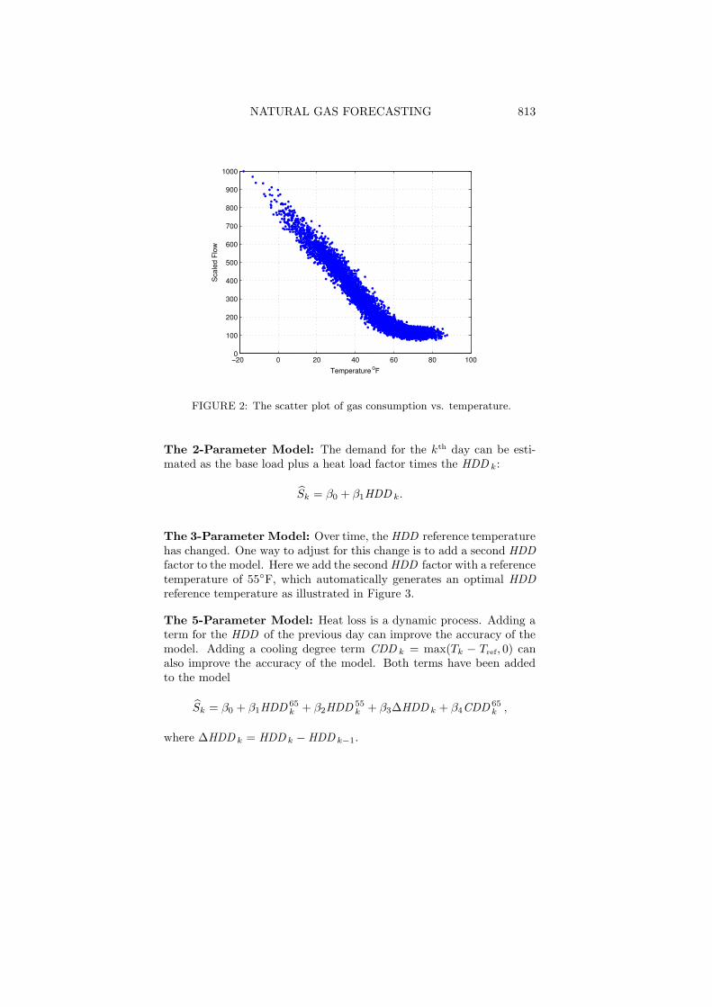
When temperatures are cold, as temperature increases, gas consump-tion decreases in a nearly linear way, although once the ambient tem-perature reaches approximately 55 to 65 degrees Fahrenheit, consump-tion levels off. Once the average temperature reaches a certain tem-perature, space heating no longer occurs; consumption levels are nearsome constant value known as base load. This nonlinear characteris-tic was observed long ago and used to define the Heating Degree Day(HDD) [3, 4, 13] as

HDD k = max(0, Tref − Tk),

where Tk is the average temperature for the kth day, and Tref is thereference temperature, historically set to 65◦F or 18◦C. Gas consump-tion versus average temperature for individual days has been plottedin Figure 2, which illustrates that gas consumption is approximatelyproportional to HDD.


−20 0 20 40 60 80 1000

100

200

300

400

500

600

700

800

900

1000

Sca

led

Flow

Temperature oF

FIGURE 2: The scatter plot of gas consumption vs. temperature.

The 2-Parameter Model: The demand for the kth day can be esti-mated as the base load plus a heat load factor times the HDD k:

Sk = β0 + β1HDD k.

The 3-Parameter Model: Over time, the HDD reference temperaturehas changed. One way to adjust for this change is to add a second HDDfactor to the model. Here we add the second HDD factor with a referencetemperature of 55◦F, which automatically generates an optimal HDDreference temperature as illustrated in Figure 3.

The 5-Parameter Model: Heat loss is a dynamic process. Adding aterm for the HDD of the previous day can improve the accuracy of themodel. Adding a cooling degree term CDD k = max(Tk − Tref, 0) canalso improve the accuracy of the model. Both terms have been addedto the model

Sk = β0 + β1HDD 65

k + β2HDD 55

k + β3∆HDD k + β4CDD 65

k ,

where ∆HDD k = HDD k − HDD k−1.


Temperature

Dem

and

55 65

FIGURE 3: Adding a second HDD term has the effect of allowing al-gorithmic adjustment of the HDD reference temperature.

3.2 Modeling wind effects Another important factor is wind, be-cause buildings lose more heat on a windy day than on a calm day. Windcould be added as another term to the models above, but then the windeffect would be the same at all temperatures, while it is well known thatthe impact of wind increases with HDD. A common method that workswell is to use Heating Degree Days adjusted for Wind (HDDW). If WSis wind speed in mph,

HDDW =

(WS + 152

160

)× HDD, WS ≤ 8

HDD, WS = 8(

WS + 72

80

)× HDD, WS > 8 .

3.3 Previous day demand Typically, the load forecasts are made forthe coming day before the current day’s gas day is complete. Thus, thecurrent day’s demand is not known. However, yesterday is over, so theflow for that day may be known. Adding this and earlier daily flowsas inputs to the forecast model, making it autoregressive, can reduceforecast error significantly.


3.4 Modeling day of the week effects Gas consumption varies bythe day of the week. For example, on weekends, as residential con-sumption increases, demand is typically more than offset by decreasedconsumption of both commercial and industrial consumption. Gas loadforecasters have used many techniques to try to capture this effect, pri-marily by adding day-of-the-week indicator model inputs.

Weekday/Weekend indicator: A binary indicator variable can beadded to the model to distinguish weekdays from weekends. That is,the variable Weekend is 1 on Saturdays and Sundays and 0 on the otherdays of the week. This term can be added to any of the models describedabove.

Friday indicator: Since the industry definition of a gas day for a Fridayincludes the Saturday morning start-up, typically demand for gas dayFriday is lower than the other weekdays, yet higher than Saturday andSunday demands. This effect varies from region to region at an LDCand certainly across the country. This effect can be accounted for bysetting the indicator variable to a number between 0 and 1 on Fridays.

Sine/cosine indicators: Periodic phenomena can be represented byFourier series [38]. The days of the week are periodic with a period ofseven days, so we can use a day-of-the-week DOW variable to representthe fundamental seven day frequency, 1 = Sunday, 2 = Monday, etc.:

sin

(2πDOW

7

), cos

(2πDOW

7

).

Seven day lag: Another technique for improving the demand forecastincludes both the demand and the temperature/HDD for the day sevendays ago, unless the day seven days earlier was a holiday.

3.5 Holidays and days around holidays Holidays and days nearholidays typically have lower demands than if the day was not a holiday.One approach that can be used with or without the above mentionedday of week adjustment is to average the residual errors in the trainingdata on specific holidays and adjust the demand forecast. For example,if, after parameterizing our model, we evaluate the model on all of theNew Years Days in the training set and calculate the forecast error asthe demand forecast minus the actual flow, and calculate the averageerrors, we can subtract this average error to adjust the forecast on NewYears Day.


Holiday adjustments: Another common way to predict gas consump-tion for a holiday is to pretend that the day is a Saturday. Days nearholidays also can be adjusted, i.e., the day before a holiday can be setto a Friday, or when a holiday falls on a Monday, set the Sunday toSaturday and set the holiday (Monday) to a Sunday. Models that usedemands from previous days are biased low on days after holidays, asthe low holiday demand is now an input to the model. This low holidaydemand can be adjusted by adding in the average error to make it actlike a non-holiday.

3.6 Other factors Many other potential factors exist, such as solar ra-diation, cloud cover, precipitation, dew point, direction of the wind, tapwater temperature, bill shock, occupancy rates, industrial productionrates, and other econometric factors, to name a few. Some of these fac-tors can be measured directly, while others cannot, or at least, cannotbe measured reasonably. Solar radiation and cloud cover affect tem-peratures throughout the day. For example, the evening temperaturedecrease is less on a cloudy day than on a clear day. Wind directionhas an effect, especially in coastal regions next to oceans or the GreatLakes. The dew point is a measure of humidity, and more gas tends tobe consumed on humid days. Precipitation measures rain and snow fall.Industrial production and other economic factors affect gas consump-tion especially in parts of the country where there is a large industrialconcentration. For example, in Michigan the economic recession causeda decrease in auto production, reducing gas consumption. Bill shocks,as experienced in 2005 when hurricanes hit the Gulf of Mexico, causepeople to turn down their thermostats in an effort to reduce their billsafter having paid a large gas bills for their prior billing period or inresponse to media coverage.

4 Data quality When building models from historical data, thedata quality of the training data set is critical. Most model fitting algo-rithms, including MLR and the ANN training methods discussed above,are designed to minimize the error standard deviation, a form of squarederror. If the training data contains errors, the model does not fit well.

Data cleaning: The best scenario is to start with good data, butenough good historical data is not always available. We can use pre-liminary demand forecast models to detect anomalous data, which canbe confirmed, and corrected or discarded before final models are devel-oped [26, 28, 39, 40].


Data disaggregation: Similarly, for some LDC’s, the only historicaldemand data available may be (approximately) monthly, although dailydemand forecasts are required. It often is possible to use preliminarydemand forecast models to disaggregate monthly data into approximatehistorical daily data before final models are developed [45]. Similartechniques can be used to give good hourly demand forecasts in thepresence of unreliable hourly flow data [35].

Number of training days: Insufficient historical data can introduceproblems in training models to predict gas consumption. When train-ing ANN’s, heuristically, ten times as many training set vector pairsas weights in the ANN are needed. Otherwise, the ANN will “memo-rize” the training vector pairs and will not generalize the trends in thedata well. This memorizing phenomena is known as over-training orover-fitting. Similar problems occur with linear regression models if thetraining data set is not large enough or sufficiently rich.

Growth in the customer base: Models are developed from a verylarge experience base, but models for an LDC are trained on historicaldata from that LDC. The most recent years of gas consumption historytend to be most relevant. The older data is not a good indication of thecurrent customer base characteristics due to both customer base growth(“growth” can be negative) and demand-side management. Because ofthis non-stationary customer base, building a model to predict demandfor the next heating season is difficult, but growth adjustments can becalculated [19, 20, 22, 25, 44].

Let us consider an example to illustrate this. Suppose a model isbuilt using data from the most recent five years from an operating areawith substantial growth. If all days in the training data set are equallyweighted, the model best predicts the load for the average customer basein the training data set. The residual errors of the model is smallest forthe middle year. The errors tend to be positive (larger predictions thanactual demand) over the first two years of the training data, and tendto be negative (smaller predictions than actual demand) over the lasttwo years of the training data. Our goal is to build a model to predictdemand for the coming heating season, but the model best predicts theheating season three years prior.

This problem can be partially overcome by “growing” the older his-torical data [12]. A simple way to grow historical data is to make itall look like it occurred during the most recent heating season. Thisis accomplished by calculating linear regression models for each heating


season. The demands from heating seasons before the most recent canbe adjusted by adding a base-load factor to each day to make the baseloads the same as the most recent season and by adding additional de-mand proportional to the HDD to each day to make the use per HDDfactor the same as the use per HDD for the most recent season. Forexample, using only 2008–2009 data, we built a 2-parameter model

Sk = β2009

0+ β2009

1HDD k,

and using only 2007–2008 data, we built a 2-parameter model

Sk = β2008

0+ β2008

1HDD k.

We then grew the 2007–2008 heating season data as

Snewk = Sk +

(β2009

0− β2008

0

)+

(β2009

1− β2008

1

)HDD k.

The “new” 2007–2008 demand data has the same base load and heatload factor as the 2008–2009 data, but it is appropriate for the weatherof 2007–2008.

Flow vs. demand: Models built using flow (consumption) data pre-dict flow. Models built using demand data predict demand. On mostdays, flow equals demand. However, on days when the LDC interruptscustomers, or injects from storage, or when a hurricane disrupts an en-tire region, the gas that flows through the city gate stations is less thanthe demand for gas.

Figure 4 shows the actual flow versus temperature for a different oper-ating area than Figure 2, which contains many interruptible customers.The “bend over” effect at colder temperatures is caused by customersbeing interrupted. To make a flow forecasting model predict demand,the historical training data must be augmented with estimated inter-rupted flow, so that the model built using this data predicts demand.

Operating areas: Forecast accuracies often can be improved by sub-dividing the region for which demand forecasts are required into smalleroperating areas and forecasting each area with separately trained mod-els. Smaller areas may benefit from more accurate average weather fore-casts, from a more homogenous customer base, or from other factors.

Multiple weather stations: Forecast accuracies often can be im-proved by using carefully tuned weighted averages of weather forecastsfrom multiple stations in or near the target operating area.


10 20 30 40 50 60 70 80 90 100100

200

300

400

500

600

700

800

900

1000

Sca

led

Flow

Temperature oF

FIGURE 4: Flow versus temperature for an operating area with inter-ruptible customers.

Generalization, interpolation, and extrapolation: Claims havebeen made that ANN’s are excellent generalizers [24, 47]; that an ANNcan learn general trends from a training data set and then can makevalid estimates for an input that it has not seen before [7, 43]. Thisis true if the input is similar to inputs in the training data, but it isfalse if the input is not close to any of the inputs in the training data.A better way to state the capabilities of an ANN is that it interpolateswell, but in general, it extrapolates unpredictably [5, 16]. In contrast,the linear regression model extrapolates very predictably [31], and inthe gas demand forecasting case, quite well.

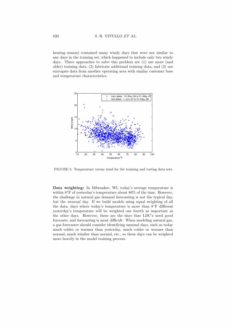
This implies that the ANN model forecasts gas demand estimateswell on days that are similar to historical days in the training set, andnot as well on days that are not similar to those in the training set.This rightly brings up concerns for demand estimations on peak daysand even uncommon days (days that are significantly colder, warmeror windier than normal, days that are much warmer or colder than theprevious day, etc.).

Figure 5 shows temperature versus wind for the training set (12 Nov.1994 to 31 May 1997) and the testing set (1 June 1997 to 31 May 1998)for an ANN trained for the 1997–1998 heating season. Even thoughthe 1997–1998 heating season was mild (El-Nino), the testing set (the


heating season) contained many windy days that were not similar toany days in the training set, which happened to include only two windydays. Three approaches to solve this problem are (1) use more (andolder) training data, (2) fabricate additional training data, and (3) usesurrogate data from another operating area with similar customer baseand temperature characteristics.

10 20 30 40 50 60 70 80 90 1000

5

10

15

20

25

Win

d (m

ph)

Temperature oF

train dates: 12−Nov−94 to 31−May−97test dates: 1−Jun−97 to 31−May−98

FIGURE 5: Temperature versus wind for the training and testing data sets.

Data weighting: In Milwaukee, WI, today’s average temperature iswithin 8◦F of yesterday’s temperature about 80% of the time. However,the challenge in natural gas demand forecasting is not the typical day,but the unusual day. If we build models using equal weighting of allthe data, days where today’s temperature is more than 8◦F differentyesterday’s temperature will be weighted one fourth as important asthe other days. However, these are the days that LDC’s need goodforecasts, and forecasting is most difficult. When modeling natural gas,a gas forecaster should consider identifying unusual days, such as todaymuch colder or warmer than yesterday, much colder or warmer thannormal, much windier than normal, etc., so these days can be weightedmore heavily in the model training process.


5 GasDay performance The following presentation of GasDayTM

forecasting results is performed on 14 different operating areas for autility in the US. The models that generated these forecasts were trainedon September 14, 2009 so results shown from October 2009 through July2010 are exclusive of the training data set. Their flow has been scaledto protect their proprietary data. Figure 6 shows the scaled flow andthe GasDayTM estimated flow for a one-day-ahead forecast for January2010.

Figure 7 shows the temperature and one-day-ahead temperature fore-casts for January, which corresponds to the flow and flow estimate inFigure 6. Figures 6 and 7 show time series for operating area one. ForJanuary 7th, 16th, 19th, and 20th, GasDayTM had large forecast errors,as shown in in Figure 6. On these days, the weather forecast error wasalso several degrees. Hence, the accuracy of GasDay’sTM forecasts aredependent on the accuracy of the weather forecasts used.

FIGURE 6: Flow and GasDayTM one-day-ahead estimated flow

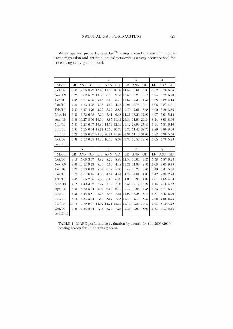
Tables 1 and 2 show Mean Absolute Percent Error (MAPE) by monthfor the 14 different operating areas. MAPE for the period of October2009 through July 2010 is also reported. Table 1 and 2 show resultsfor the Linear Regression (LR), Artificial Neural Network (ANN), andGasDay’sTM combined estimate (GD). We empirically observe the sameconclusions Bates and Granger [6] and Dickinson [14] assert. For the


FIGURE 7: Temperature and one-day-ahead temperature forecast

period of October 2009 through July 2010 on 11 of 14 operating areas,GasDay’sTM estimate is better than the best of the two component mod-els, and all 14 GasDay estimates are better than the worst componentmodel. Operating areas 3, 9, and 14 contain large concentrations of in-dustrial customers that have less heating load sensitivity, making themharder to forecast.

6 Summary In this paper, we have emphasized the importancefor LDCs to make accurate natural gas demand forecasts and the finan-cial consequences to their customers if they do not. Additionally, wedescribed two important model fitting algorithms used by GasDayTM

to forecast daily natural gas demand: multiple linear regression andartificial neural networks. The impacts of temperature, wind, priorday weather, previous day demands, day of the week, and holidays ongas consumption have been discussed, along with common data qualityissues such as the length of the training data set, the differences be-tween flow and demand, and customer base growth are also discussed.In addition, we described the models and variables that are used byGasDayTM to forecast LDCs consumption and the data quality issuesthat must be addressed before good models can be trained. A surveyof GasDayTM performance results show that GasDayTM forecasts gasconsumption well.


When applied properly, GasDayTM using a combination of multiplelinear regression and artificial neural networks is a very accurate tool forforecasting daily gas demand.

1 2 3 4

Month LR ANN GD LR ANN GD LR ANN GD LR ANN GD

Oct.’09 8.83 9.36 8.72 12.40 11.53 10.02 14.59 16.61 13.30 6.52 5.76 6.06

Nov.’09 5.28 5.52 5.52 10.33 8.79 9.57 17.58 15.26 15.18 6.24 6.79 6.20

Dec.’09 4.48 5.21 5.05 5.45 5.09 5.72 11.62 14.33 11.54 3.68 3.89 4.13

Jan.’10 4.80 4.73 4.28 5.38 4.92 4.73 10.94 13.75 12.71 4.06 3.87 4.01

Feb.’10 7.57 6.47 4.76 3.22 3.22 3.86 9.79 7.61 8.68 4.90 3.29 3.86

Mar.’10 6.30 6.72 6.68 7.29 7.41 6.48 14.31 13.20 12.90 4.97 5.01 5.12

Apr.’10 9.86 10.27 8.66 10.64 8.65 11.41 29.84 31.99 29.34 8.14 8.08 8.66

May’10 5.81 6.23 6.07 10.84 14.79 12.16 31.12 28.93 27.43 6.94 5.51 6.10

Jun.’10 5.82 5.35 6.44 15.77 15.53 10.70 40.26 31.46 32.73 9.29 8.80 8.66

Jul.’10 5.29 5.36 6.27 20.23 20.81 11.99 32.91 31.13 31.67 5.82 5.96 5.46

Oct.’09 6.39 6.52 6.25 10.20 10.13 8.69 21.33 20.50 19.59 6.05 5.70 5.83

to Jul.’10

5 6 7 8

Month LR ANN GD LR ANN GD LR ANN GD LR ANN GD

Oct.’09 3.16 5.06 3.67 9.82 8.26 8.86 12.54 10.04 9.25 5.58 5.87 6.23

Nov.’09 8.66 13.12 9.73 5.30 5.06 4.42 11.21 11.98 8.86 11.66 9.65 9.78

Dec.’09 6.28 5.33 6.13 5.89 6.12 5.83 6.47 10.25 5.66 5.40 5.41 5.84

Jan.’10 5.78 6.51 6.15 4.60 4.34 4.41 4.79 4.81 4.01 3.42 2.35 2.70

Feb.’10 2.48 3.56 2.95 5.60 5.63 5.25 4.06 3.95 4.07 4.81 4.68 4.83

Mar.’10 4.18 4.40 3.02 7.27 7.12 7.08 8.51 12.12 8.22 4.14 4.16 4.62

Apr.’10 5.66 5.72 5.34 6.04 6.09 6.19 9.42 12.95 7.38 6.53 6.77 6.71

May’10 5.36 6.45 5.81 8.26 7.45 7.64 12.92 13.28 13.73 6.37 6.42 6.20

Jun.’10 3.16 3.33 3.44 7.30 8.02 7.38 11.19 7.19 8.30 7.66 7.96 6.23

Jul.’10 10.78 9.79 9.97 14.92 14.21 15.36 11.75 9.86 10.47 7.61 8.10 4.29

Oct.’09 5.58 6.34 5.64 7.53 7.25 7.27 9.33 9.69 8.03 6.31 6.13 5.73

to Jul.’10

TABLE 1: MAPE performance evaluation by month for the 2009/2010heating season for 14 operating areas.


9 10 11

Month LR ANN GD LR ANN GD LR ANN GD

Oct.’09 8.26 7.04 5.82 9.47 8.35 7.03 14.40 14.87 13.90

Nov.’09 7.02 7.57 6.39 8.11 10.36 9.51 8.41 9.96 8.09

Dec.’09 5.26 4.61 5.16 6.77 10.34 7.04 5.00 5.21 5.89

Jan.’10 5.33 4.99 5.17 4.86 4.89 5.70 4.48 4.25 4.32

Feb.’10 7.93 6.32 6.21 4.53 3.77 4.31 6.73 5.69 4.97

Mar.’10 11.66 9.61 8.68 8.70 8.84 7.80 5.78 5.88 6.45

Apr.’10 15.33 10.48 9.44 14.01 18.08 9.89 10.41 9.95 10.12

May’10 29.63 23.11 19.27 12.98 11.39 6.40 6.01 6.05 6.85

Jun.’10 28.87 26.20 17.65 13.83 21.50 8.54 6.55 5.72 6.61

Jul.’10 21.91 23.31 13.01 14.48 14.25 13.34 4.81 4.82 4.89

Oct.’09 14.15 12.36 9.70 9.80 11.20 7.98 7.25 7.24 7.22

to Jul.’10

12 13 14

Month LR ANN GD LR ANN GD LR ANN GD

Oct.’09 10.67 9.18 8.09 9.68 8.99 9.65 23.26 25.44 16.14

Nov.’09 6.33 5.28 5.58 11.68 10.73 9.19 16.30 17.44 16.70

Dec.’09 4.17 3.56 3.48 4.63 4.61 4.86 18.08 19.91 19.71

Jan.’10 4.59 4.38 4.02 3.92 3.76 4.17 9.49 10.14 8.28

Feb.’10 3.42 3.39 4.22 5.99 6.70 6.20 9.28 10.02 8.29

Mar.’10 6.39 6.59 5.49 5.67 5.77 5.99 10.98 10.45 9.66

Apr.’10 8.43 9.38 7.24 10.07 7.81 8.54 25.01 19.66 19.19

May’10 7.48 8.53 3.99 5.68 5.67 5.53 18.99 14.47 14.95

Jun.’10 8.13 7.20 4.92 4.56 4.67 4.59 17.20 15.26 16.04

Jul.’10 10.77 8.30 5.06 4.95 4.79 4.65 19.22 14.00 15.42

Oct.’09 7.07 6.60 5.21 6.67 6.33 6.33 16.83 16.00 14.47

to Jul.’10

TABLE 2: MAPE performance evaluation by month for the 2009/2010heating season for 14 operating areas.

REFERENCES

1. American Gas Association, (2010), http://www.aga.org.2. J. S. Armstrong, Principles of Forecasting a Handbook for Researchers and

Practitioners, Kluwer Academic Publishers, Boston, 2001.3. J. G. Asbury, C. Maslowski and R. O. Mueller, Solar availability for winter

space heating: an analysis of SOLMET data, 1953 to 1975, Science 206(4419)(1979), 679–681.


4. D. G. Baker, Effect of obervation time on mean temperature estimation, J.Appl. Meteor.14(4) (1975), 471–476.

5. E. Barnard and L. F. A. Wessels, Extrapolation and interpolation in neuralnetwork classifiers, IEEE Control Syst. Mag. 12(5) (1992), 50–53.

6. J. M. Bates and C. W. J. Granger, The combination of forecasts, Oper. Res.Q. 20 (1969), 451–468.

7. D. S. Broomhead and D. Lowe, Multivariable functional interpolation andadaptive networks, Complex Syst. 2(3) (1988), 321–355.

8. R. H. Brown, I. Matin and X. Feng, Development of feed-forward neural net-work models for gas short-term load forecasting, 222–229, Proc. Adaptive Con-trol Systems Technology Symposium; Theme: High Tech Controls for Energyand Environment, Pittsburgh, PA, 1994.

9. R. H. Brown, I. Matin, P. Kharouf and L. P. Piessens, Development of artificialneural network models to predict daily gas consumption, AGA Forecasting Rev.5 (1996), 1–22.

10. R. H. Brown, T. M. Richardson and J. E. Buchanan, Forecasting daily sendoutdemand with artificial neural networks, 131–139, Amer. Gas Assoc. OperatingSection Pre-Print Proc., Cleveland, OH, 1999.

11. R. H. Brown, OK, who is playing with the thermostat?, Gas Forecaster’s Fo-rum, Albuquerque, NM, October 2003.

12. R. H. Brown, Y. Li, B. Pang, S. R. Vitullo and G. F. Corliss, Detrendingdaily natural gas demand data using domain knowledge, 10, Proc. 30th Int.Symposium on Forecasting, San Diego, CA, 2010.

13. P. M. Dare, A study of the severity of the midwestern winters of 1977 and1978 using heating degree days determined from both measured and wind chilltemperatures, Bull. Amer. Meteor. Soc. 62(7) (1981), 974–982.

14. J. P. Dickinson, Some statistical results in the combination of forecasts, Oper.Res. Q. 24(2) (1998).

15. N. R. Draper and H. Smith, Applied Regression Analysis, 3rd ed., John Wiley& Sons, New York, 1998.

16. W. Duch and G. H. F. Diercksen, Neural networks as tools to solve problemsin physics and chemistry, Comput. Phys. Comm. 82(2–3) (1994), 91–103.

17. Energy and Environmental Analysis Inc., The Impacts of Recent Hurricaneson U.S. Gas Markets for the Upcoming Winter, Technical Report, 2005.

18. A. S. Goldberger, Topics in Regression Analysis, Macmillan, New York, 1968.19. T. Haida and S. Muto, Regression based peak load forecasting using a trans-

formation technique, IEEE Trans. Power Syst. 9(4) (1994), 1788–1794.20. T. Haida, S. Muto, Y. Takahashi and Y. Ishi, Peak load forecasting using

multiple-year data with tend data processing techniques, Electr. Eng. Japan124 (1998), 7–16.

21. S. Halim, Selection of Inputs for Generating Combinatorial Daily Natural GasDemand Forecasts, M.S. thesis Marquette University Department of Electricaland Computer Engineering, Milwaukee, WI, 2004.

22. M. He, Annual Transformation Algorithm for Hourly Data in Natural GasConsumption, M.S. thesis, Marquette University Department of Electrical andComputer Engineering, Milwaukee, WI, 2007.

23. J. J. Hopfield, Neural networks and physical systems with emergent collectivecomputational abilities, Proc. Nat. Acad. Sci. USA 79 (1982), 2554–2558.

24. K. Hornick, M. Stinchcombe and H. White, Multilayer feedforward networksare universal approximators, Neural Networks 2 (1989), 359–366.

25. D. Hughes and R. H. Brown, Analysis of customer base growth over time, GasForecaster’s Forum, Greensboro, NC, 2002.

26. R. O. Kennedy, Detecting Outliers and Meter Anomalies in Natural Gas Cus-tomer Flow Data, M.S. thesis, Marquette University Department of Electricaland Computer Engineering, Milwaukee, WI, 2006.


27. A. Khotanzad, H. Elragal and T. L. Lu, Combination of artificial neural net-work forecasters for prediction of natural gas consumption, IEEE Trans. NeuralNetworks 11 (2000), 464–473.

28. S. Kiware, Detection of Outlies in Time Series Data, M.S. thesis, MarquetteUniversity Department of Mathematics, Statistics, and Computer Science, Mil-waukee, WI, 2010.

29. R. R. Levary and B. V. Dean, A natural gas model under uncertainty in de-mand, Oper. Res. 28(6) (1980), 1360–1374.

30. H. L. Lim and R. H. Brown, Hourly gas load forecasting model input factoridentification using a genetic algorithm, 670–673, Proc. 44th IEEE MidwestSymposium on Circuits and Systems, Dayton, OH, 2001.

31. H. Lohninger, Evaluation of neural networks based on radial basis functionsand their application to the prediction of boiling points from structural param-eters, J. Chem. Information Comput. Sci. 33(5) (1993), 736–744.

32. F. K. Lyness, Gas demand forecasting, The Statistician 33(1) (1984).33. F. K. Lyness, Consistent forecasting of severe winter gas demand, J. Oper.

Res. Soc. 32(5) (1981), 347–459.34. B. M. Marx, Forecasting Daily Processing Tomato Harvest Tonnage in Califor-

nia, M.S. thesis, Marquette University Department of Electrical and ComputerEngineering, Milwaukee, WI, 2004.

35. B. Marx, Fitting a Continuous Profile to Hourly Natural Gas Flow Data,Ph.D. thesis, Marquette University Department of Electrical and ComputerEngineering, Milwaukee, WI, 2007.

36. W. S. McCulloch and W. Pitts, A logical calculus of the ideas immenent innervous activity, Bull. Math. Biophys. 5 (1943), 115–133.

37. M. L. Minsky and S. A. Papert, Perceptrons, The MIT Press, Cambridge, MA,1969. (Expanded ed. 1990.)

38. A. V. Oppenheim, A. S. Willsky and S. H. Nawab, Signals and Sytems 2nded., Prentice Hall, Upper Saddle, NJ, 1997.

39. Ronald K. Pearson, Outliers in process modeling and identification, IEEETrans.Control Syst. Technol. 10(1) (2002), 55–63.

40. Ronald K. Pearson, Mining Imperfect Data, SIAM, U.S.A., 2005.41. F. Rosenblatt, Principles of Neurodynamics: Perceptrons and the Theory of

Brain Mechanisms, Spartan, New York, 1962.42. D. E. Rummelhart, G. E. Hinton, and R. J. Williams, Learning internal repre-

sentations by error propagation, Parallel Distributed Processing, D. E. Rum-melhart, J. L. McClelland, and the PDP Research Group, The MIT Press,Cambridge, MA, 1986, 318–362.

43. D. Suter, Neural net surface interpolation, Proceedings of the 1987 Interna-tional Conference on Systems, Man, and Cybernetics, IEEE 1 (1987), 118–123,New York, NY., USA.

44. A. Taware, Forecasting and Identification Methods Applied to Gas Load Esti-mation Problems, M.S. thesis, Marquette University Department of Electricaland Computer Engineering, Milwaukee, WI, 1998.

45. S. R. Vitullo, Disaggregating Interval Time-Series Data Applied to NaturalGas Flow Estimation, M.S. thesis, Marquette University Department of Elec-trical and Computer Engineering, Milwaukee, WI, 2007.

46. T. H. Welch, J. G. Smith, J. P. Rix and R. D. Reader, Meeting seasonal peakdemand for natural gas, Operational Research Quarterly 22 (1971), 93–106.

47. A. Weiland and R. Leighton, Geometric analysis of neural network capabili-ties, 385–392, IEEE First International Conference on Neural Networks, SOSPrinting 3, San Diego, CA, 1987.


Department of Electrical and Computer Engineering

P. O. Box 1881, Marquette University, Milwaukee, WI 53201–1881

E-mail address: [email protected]




mathematical models for natural gas forecasting · pdf filemathematical models for natural gas...

Documents