Mathematical Modeling

Williams, Gueret a. o.

Tony Hürlimann

Department of Informatics

University of Fribourg

CH – 1700 Fribourg (Switzerland)

tony.huerlimann@unifr.ch

January 4, 2020

Copyright © 2019All rights reserved. Department of InformaticsUniversity of FribourgCH-1700 Fribourg SwitzerlandEmail: tony.huerlimann@unifr.chWWW: http://www.virtual-optima.com

i

ii

CONTENTS

1 Introduction 31.1 Model and Related Concepts . . . . . . . . . . . . . . . . . . 41.2 The Model Building Process . . . . . . . . . . . . . . . . . . . 61.3 The Modeling Language LPL . . . . . . . . . . . . . . . . . . 101.4 Mathematical Notation . . . . . . . . . . . . . . . . . . . . . 16

1.4.1 Set-Names versus Index-Names . . . . . . . . . . . . . 161.4.2 Logic-mathematical Notation . . . . . . . . . . . . . . 171.4.3 Logical Operators . . . . . . . . . . . . . . . . . . . . 18

2 Problems from William's Book 192.1 Food Manufacture I (will01) . . . . . . . . . . . . . . . . . . 202.2 Food Manufacture II (will02) . . . . . . . . . . . . . . . . . . 212.3 Factory planning I (will03) . . . . . . . . . . . . . . . . . . . 232.4 Factory planning II (will04) . . . . . . . . . . . . . . . . . . . 242.5 Manpower Planning (will05) . . . . . . . . . . . . . . . . . . 262.6 Refinery Optimization I (will06) . . . . . . . . . . . . . . . . 282.7 Refinery Optimization II (will06a) . . . . . . . . . . . . . . . 312.8 Mining (will07) . . . . . . . . . . . . . . . . . . . . . . . . . 332.9 Farm Planning (will08) . . . . . . . . . . . . . . . . . . . . . 342.10 Economic Planning (will09) . . . . . . . . . . . . . . . . . . . 362.11 Decentralization (will10) . . . . . . . . . . . . . . . . . . . . 382.12 Curve Fitting (linear) (will11) . . . . . . . . . . . . . . . . . . 402.13 Curve Fitting (quadratic) (will11a) . . . . . . . . . . . . . . . 432.14 Logical Design (will12) . . . . . . . . . . . . . . . . . . . . . 442.15 Market Sharing I (will13) . . . . . . . . . . . . . . . . . . . . 462.16 Market Sharing II: (will13a) . . . . . . . . . . . . . . . . . . . 482.17 Opencast Mining I (will14) . . . . . . . . . . . . . . . . . . . 502.18 Opencast Mining II (will14a) . . . . . . . . . . . . . . . . . . 52

iii

2.19 Opencast Mining III (will14b) . . . . . . . . . . . . . . . . . . 542.20 Tariff Rates (Power Generation) (will15) . . . . . . . . . . . . 562.21 Hydro power (will16) . . . . . . . . . . . . . . . . . . . . . . 582.22 T3-dimensional Noughts and Crosses (will17) . . . . . . . . . 602.23 Optimizing a Constraint (will18) . . . . . . . . . . . . . . . . 622.24 Distribution I (will19) . . . . . . . . . . . . . . . . . . . . . . 642.25 Distribution II (will19a) . . . . . . . . . . . . . . . . . . . . . 662.26 Depot Location (Distribution 2) (will20) . . . . . . . . . . . . 682.27 Agricultural Pricing I (will21) . . . . . . . . . . . . . . . . . . 702.28 Agricultural Pricing II (will21a) . . . . . . . . . . . . . . . . . 732.29 Efficiency Analysis (EA) (will22) . . . . . . . . . . . . . . . . 742.30 Milk Collection (will23) . . . . . . . . . . . . . . . . . . . . . 762.31 Yield Management (will24) . . . . . . . . . . . . . . . . . . . 782.32 Car Rental I (will25) . . . . . . . . . . . . . . . . . . . . . . . 802.33 Car Rental II (will26) . . . . . . . . . . . . . . . . . . . . . . 832.34 Lost Baggage Distribution (will27) . . . . . . . . . . . . . . . 862.35 Protein Folding (will28) . . . . . . . . . . . . . . . . . . . . . 882.36 Protein Comparison (will29) . . . . . . . . . . . . . . . . . . 902.37 Product Mix I (willi005) . . . . . . . . . . . . . . . . . . . . . 912.38 Product Mix II (willi005a) . . . . . . . . . . . . . . . . . . . . 922.39 Vegetable Oil Blending (willi008) . . . . . . . . . . . . . . . . 932.40 Multi-Plant Planning (willi055) . . . . . . . . . . . . . . . . . 942.41 Transportation (willi082) . . . . . . . . . . . . . . . . . . . . 952.42 Production Planning (willi085) . . . . . . . . . . . . . . . . . 962.43 Minimum Cost Flow (willi090) . . . . . . . . . . . . . . . . . 972.44 Shortest Path Problem (willi093) . . . . . . . . . . . . . . . . 982.45 Maximum Flow (willi094) . . . . . . . . . . . . . . . . . . . . 992.46 Critical Path (willi095) . . . . . . . . . . . . . . . . . . . . . 1002.47 A Small QP (willi142) . . . . . . . . . . . . . . . . . . . . . . 1012.48 LP-relaxtion versus IP-solution (willi155) . . . . . . . . . . . 1022.49 LP-relaxtion versus 0-1-IP-solution (willi155z) . . . . . . . . . 105

3 Problems from the Gueret Book 1073.1 Animal food production (guer04-2) . . . . . . . . . . . . . . . 1083.2 Production of alloys (guer04-3) . . . . . . . . . . . . . . . . . 1093.3 Refinery (guer04-4) . . . . . . . . . . . . . . . . . . . . . . . 1103.4 Cane Sugar Production (guer04-5) . . . . . . . . . . . . . . . 1113.5 Opencast Mining (guer04-6) . . . . . . . . . . . . . . . . . . 1123.6 Production of Electricity (guer04-7) . . . . . . . . . . . . . . . 1133.7 Stadium Construction (guer05-2) . . . . . . . . . . . . . . . . 1143.8 Flow-shop Scheduling (guer05-3) . . . . . . . . . . . . . . . . 1173.9 Job Shop: non-generic version (guer05-4a) . . . . . . . . . . . 1193.10 Job Shop: generic version (guer05-4b) . . . . . . . . . . . . . 1203.11 Sequencing jobs on a bottleneck machine (guer05-5) . . . . . . 1213.12 Paint production (guer05-6) . . . . . . . . . . . . . . . . . . . 1223.13 Assembly line balancing (guer05-7) . . . . . . . . . . . . . . . 123

iv

3.14 Planning the production of bicycles (guer06-2) . . . . . . . . . 1243.15 Production of drinking glasses (guer06-3) . . . . . . . . . . . 1253.16 Material Requirement Planning (guer06-4) . . . . . . . . . . . 1263.17 Production of elec. components (guer06-5) . . . . . . . . . . . 1273.18 Production of fiberglass (guer06-6) . . . . . . . . . . . . . . . 1283.19 Assign prod batches to machines (guer06-7) . . . . . . . . . . 1293.20 Wagon load balancing (guer07-2) . . . . . . . . . . . . . . . . 1303.21 Barge loading (guer07-3) . . . . . . . . . . . . . . . . . . . . 1313.22 Tank loading (guer07-4) . . . . . . . . . . . . . . . . . . . . . 1323.23 Backing up files (guer07-5) . . . . . . . . . . . . . . . . . . . 1333.24 Cutting sheet metal (guer07-6) . . . . . . . . . . . . . . . . . 1343.25 Cutting steel bars for desk legs (guer07-7) . . . . . . . . . . . 1353.26 Car rental (guer08-2) . . . . . . . . . . . . . . . . . . . . . . 1363.27 Choosing the mode of transport (guer08-3) . . . . . . . . . . . 1373.28 Depot location (guer08-4) . . . . . . . . . . . . . . . . . . . . 1383.29 Heating oil delivery (guer08-5) . . . . . . . . . . . . . . . . . 1393.30 Combining diff modes of transport (guer08-6) . . . . . . . . . 1403.31 Fleet planning for vans (guer08-7) . . . . . . . . . . . . . . . 1413.32 Flight connections at a hub (guer09-2) . . . . . . . . . . . . . 1423.33 Composing flight crews (guer09-3) . . . . . . . . . . . . . . . 1433.34 Scheduling flight langings (guer09-4) . . . . . . . . . . . . . . 1443.35 Airline hub location (guer09-5) . . . . . . . . . . . . . . . . . 1453.36 Planning a flight tour (guer09-6) . . . . . . . . . . . . . . . . 1463.37 Network reliability (guer10-2) . . . . . . . . . . . . . . . . . 1473.38 Dimensioning of a mobile phone network (guer10-3) . . . . . 1483.39 Routing tlephone calls (guer10-4) . . . . . . . . . . . . . . . . 1493.40 Construction of a cabled networkt (guer10-5) . . . . . . . . . 1503.41 Scheduling of telecomm. via satellite (guer10-6) . . . . . . . . 1513.42 Localisation of GSM transmitters (guer10-7) . . . . . . . . . . 1523.43 Choice of loans (guer11-2) . . . . . . . . . . . . . . . . . . . 1533.44 Publicity campaign (guer11-3) . . . . . . . . . . . . . . . . . 1543.45 Portfolio selection (guer11-4) . . . . . . . . . . . . . . . . . . 1553.46 Finacing an early retirment scheme (guer11-5) . . . . . . . . . 1563.47 Family budget (guer11-6) . . . . . . . . . . . . . . . . . . . . 1573.48 Choice of expansion projects (guer11-7) . . . . . . . . . . . . 1583.49 Mean variance portfolio (guer11-8) . . . . . . . . . . . . . . . 1593.50 Assigning personnel to machines (guer12-2) . . . . . . . . . . 1603.51 Scheduling nurses (guer12-3) . . . . . . . . . . . . . . . . . . 1613.52 Establishing a college timetable (guer12-4) . . . . . . . . . . . 1623.53 Exam scheduling (guer12-5) . . . . . . . . . . . . . . . . . . 1633.54 Personnel assignment (guer12-6) . . . . . . . . . . . . . . . . 1643.55 Personnel at a construction site (guer12-7) . . . . . . . . . . . 1663.56 Water conveyance mamangement (guer13-2) . . . . . . . . . . 1673.57 CCTV surveillance (guer13-3) . . . . . . . . . . . . . . . . . . 1683.58 Rigging elections (guer13-4) . . . . . . . . . . . . . . . . . . 169

v

3.59 Gritting roads (guer13-5) . . . . . . . . . . . . . . . . . . . . 1703.60 Location of income tax offices (guer13-6) . . . . . . . . . . . . 1733.61 Efficiency of hospitals (guer13-7) . . . . . . . . . . . . . . . . 1743.62 MasterMind (guer14-2) . . . . . . . . . . . . . . . . . . . . . 1753.63 Probleme de logique sur le marathon de Paris (guer14-3) . . . 1763.64 Chercheurs dans un Congres (guer14-4) . . . . . . . . . . . . 1773.65 Grille et jetons (guer14-5) . . . . . . . . . . . . . . . . . . . . 1783.66 Partage de tonneaux entre des neveux (guer14-6) . . . . . . . 1793.67 Le probleme des n reines (guer14-7) . . . . . . . . . . . . . . 180

4 Various Textbooks 1814.1 Forestry Production Planning (forestry) . . . . . . . . . . . . 1814.2 Wyndor Glass Company (hill03-1-1) . . . . . . . . . . . . . . 1844.3 Mary’s Radiation Therapy (hill03-4-1) . . . . . . . . . . . . . 1854.4 Kibbutzim Crop Allocation (hill03-4-2) . . . . . . . . . . . . . 1864.5 Nori/Leets Air Pollution (hill03-4-3) . . . . . . . . . . . . . . 1874.6 Save-It Company (hill03-4-4) . . . . . . . . . . . . . . . . . . 1884.7 Save-It Company (hill03-4-4b) . . . . . . . . . . . . . . . . . 1894.8 Union Airways Personnel (hill03-4-5) . . . . . . . . . . . . . . 1904.9 Distribution Unlimited (hill03-4-6) . . . . . . . . . . . . . . . 1914.10 Wyndor Glass (hill07-1-1) . . . . . . . . . . . . . . . . . . . . 1924.11 Upper Bound (hill07-3-1) . . . . . . . . . . . . . . . . . . . . 1934.12 Goal Programming (hill07-5-1) . . . . . . . . . . . . . . . . . 1944.13 P-T Company (hill08-1-1) . . . . . . . . . . . . . . . . . . . . 1954.14 Northern Airplane (hill08-1-2) . . . . . . . . . . . . . . . . . 1964.15 Metro Water (hill08-1-3) . . . . . . . . . . . . . . . . . . . . . 1974.16 Job Shop Company (hill08-3-1) . . . . . . . . . . . . . . . . . 1984.17 Better Products Company (hill08-3-2a) . . . . . . . . . . . . . 1994.18 Better Products Company (hill08-3-2b) . . . . . . . . . . . . . 2004.19 Shortest Path (hill09-3-1) . . . . . . . . . . . . . . . . . . . . 2014.20 Maximum Flow (hill09-5-1) . . . . . . . . . . . . . . . . . . . 2024.21 Minimum Cost (hill09-6-1) . . . . . . . . . . . . . . . . . . . 2034.22 Critical Path (hill10-1-1) . . . . . . . . . . . . . . . . . . . . . 2044.23 Crashing (hill10-5-1) . . . . . . . . . . . . . . . . . . . . . . . 2054.24 Calif. Manufacturing (hill12-1-1) . . . . . . . . . . . . . . . . 2064.25 Production Rates (hill12-4-1) . . . . . . . . . . . . . . . . . . 2074.26 TV Spots (hill12-4-2a) . . . . . . . . . . . . . . . . . . . . . . 2084.27 TV Spots (hill12-4-2b) . . . . . . . . . . . . . . . . . . . . . . 2094.28 Crew Assignments (hill12-4-3) . . . . . . . . . . . . . . . . . 2104.29 Nonlinear constraint (hill13-2-1) . . . . . . . . . . . . . . . . 2114.30 Nonlinear Objective (hill13-2-2) . . . . . . . . . . . . . . . . . 2124.31 Nonlinear Objective 2 (hill13-2-3) . . . . . . . . . . . . . . . . 2134.32 Convex Programming (hill13-9-1) . . . . . . . . . . . . . . . 2144.33 Odds And Even (hill14-1-1) . . . . . . . . . . . . . . . . . . . 2154.34 Political Variaton 1 (hill14-2-1) . . . . . . . . . . . . . . . . . 2164.35 Political Variation 2 (hill14-2-2) . . . . . . . . . . . . . . . . . 217

vi

4.36 Political Variation 3 (hill14-2-3) . . . . . . . . . . . . . . . . . 2184.37 School Board Scheduling (hillC3-1) . . . . . . . . . . . . . . . 2194.38 Manufacturing (hillP3-1-3) . . . . . . . . . . . . . . . . . . . 2204.39 TV Manufacturing (hillP3-1-4) . . . . . . . . . . . . . . . . . 2214.40 Resource PQ (hillP3-1-5) . . . . . . . . . . . . . . . . . . . . 2224.41 Insurance (hillP3-1-6) . . . . . . . . . . . . . . . . . . . . . . 2234.42 Auto Spare Parts (hillP3-1-7) . . . . . . . . . . . . . . . . . . 2244.43 Resource QRS (hillP3-2-1) . . . . . . . . . . . . . . . . . . . . 2254.44 Invest Venture (hillP3-2-3) . . . . . . . . . . . . . . . . . . . 2264.45 Investment (hillP3-4-10) . . . . . . . . . . . . . . . . . . . . . 2274.46 Investor ABCD (hillP3-4-11) . . . . . . . . . . . . . . . . . . 2284.47 Alloy Blending (hillP3-4-12) . . . . . . . . . . . . . . . . . . . 2294.48 Computer Fac Oper Assignment (hillP3-4-13) . . . . . . . . . 2304.49 Warehouse Storage (hillP3-4-14) . . . . . . . . . . . . . . . . 2314.50 Paper Manufacturing (hillP3-4-15) . . . . . . . . . . . . . . . 2324.51 Steak-Potato Diet (hillP3-4-6) . . . . . . . . . . . . . . . . . . 2334.52 Pig Feed Blending (hillP3-4-7) . . . . . . . . . . . . . . . . . 2344.53 Plant Production Planning (hillP3-4-8) . . . . . . . . . . . . . 2354.54 Cargo Plane Planning (hillP3-4-9) . . . . . . . . . . . . . . . . 2364.55 MidWest Grain Elevator (midwest) . . . . . . . . . . . . . . . 2374.56 Fertilizer (murty2-1) . . . . . . . . . . . . . . . . . . . . . . . 2424.57 Gasoline Blending (murty2-2) . . . . . . . . . . . . . . . . . . 2434.58 Diet Problem (murty2-3) . . . . . . . . . . . . . . . . . . . . 2444.59 Transportation (murty2-4) . . . . . . . . . . . . . . . . . . . . 2454.60 Marriage Problem (murty2-5) . . . . . . . . . . . . . . . . . . 2464.61 Multi-Period Planning (murty2-6) . . . . . . . . . . . . . . . 2474.62 Breck and Dapper (shapiro1-1) . . . . . . . . . . . . . . . . . 2484.63 DowPont Chemical (shapiro1-2) . . . . . . . . . . . . . . . . 2494.64 Portfolio Selection (shapiro1-3) . . . . . . . . . . . . . . . . . 2504.65 Portfolio Selection (shapiro1-3b) . . . . . . . . . . . . . . . . 2514.66 Transportation (shapiro1-4) . . . . . . . . . . . . . . . . . . . 2524.67 Multi-Period Scheduling (shapiro1-5) . . . . . . . . . . . . . 2534.68 Giapetto Wood Carving (winst3-1-1) . . . . . . . . . . . . . . 2554.69 Giapetto Wood Carving II (winst3-1-1s) . . . . . . . . . . . . 2564.70 Dorian Advertising (winst3-2-2) . . . . . . . . . . . . . . . . 2574.71 Dorian Advertising (winst3-2-2s) . . . . . . . . . . . . . . . . 2584.72 Auto Company (winst3-3-3) . . . . . . . . . . . . . . . . . . 2594.73 Auto Company (winst3-3-3s) . . . . . . . . . . . . . . . . . . 2604.74 Auto Company (infeasible) (winst3-3-4) . . . . . . . . . . . . 2614.75 Unbounded Problem (winst3-3-5) . . . . . . . . . . . . . . . 2624.76 Diet Problem (winst3-4-6) . . . . . . . . . . . . . . . . . . . . 2634.77 Diet Problem (winst3-4-6s) . . . . . . . . . . . . . . . . . . . 2644.78 Star Oil (winst3-6-8) . . . . . . . . . . . . . . . . . . . . . . . 2654.79 Semicond Eletronics (winst3-7-9) . . . . . . . . . . . . . . . . 2664.80 Rylon Corporation (winst3-9-11) . . . . . . . . . . . . . . . . 268

vii

4.81 Sailco (winst3-10-12) . . . . . . . . . . . . . . . . . . . . . . 2704.82 Farmer Jones (winstP3-1-1) . . . . . . . . . . . . . . . . . . . 2714.83 Farmer Jones (winstP3-1-1s) . . . . . . . . . . . . . . . . . . 2724.84 Truck Corporation (winstP3-1-4) . . . . . . . . . . . . . . . . 2734.85 Product-Mix (Truck Co) (winstP3-1-4s) . . . . . . . . . . . . . 2744.86 Leary Chemical (winstP3-2-3) . . . . . . . . . . . . . . . . . . 2754.87 Chemical Product Processes (winstP3-2-3s) . . . . . . . . . . 2764.88 Furniture Corporation (winstP3-2-5) . . . . . . . . . . . . . . 2774.89 Product-Mix (Furniture Corporation) (winstP3-2-5s) . . . . . . 2784.90 Money Manager (winstP3-3-10s) . . . . . . . . . . . . . . . . 2794.91 Momiss River Pollution (winstP3-4-1) . . . . . . . . . . . . . 2804.92 US Lab (winstP3-4-2) . . . . . . . . . . . . . . . . . . . . . . 2814.93 Diet Problem (winstP3-4-3) . . . . . . . . . . . . . . . . . . . 2824.94 Gold Mining (winstP3-4-4) . . . . . . . . . . . . . . . . . . . 2834.95 Capital Budget (winstP3-6-2) . . . . . . . . . . . . . . . . . . 2844.96 Blending Candy (winstP3-8-1) . . . . . . . . . . . . . . . . . 2854.97 Blending Oranges (winstP3-8-2) . . . . . . . . . . . . . . . . 2864.98 Blending Portfolio (winstP3-8-3) . . . . . . . . . . . . . . . . 2874.99 Blending Investments (winstP3-8-4) . . . . . . . . . . . . . . 2884.100Blending Oils (winstP3-8-5) . . . . . . . . . . . . . . . . . . . 2894.101Blending Oils (winstP3-8-5b) . . . . . . . . . . . . . . . . . . 2904.102Blending fertilizer (winstP3-8-6) . . . . . . . . . . . . . . . . 2914.103Blending chemicals (winstP3-8-7) . . . . . . . . . . . . . . . . 2924.104Highland TV and Radio (winstP3-8-8) . . . . . . . . . . . . . 2934.105Production Process (Sunco Oil) (winstP3-9-1) . . . . . . . . . 2944.106Production Process (winstP3-9-2) . . . . . . . . . . . . . . . . 2964.107Production Process (Rylon Corp.) (winstP3-9-3) . . . . . . . . 2974.108Production Process (winstP3-9-5) . . . . . . . . . . . . . . . . 2994.109Production Process (Daisy Drug) (winstP3-9-6) . . . . . . . . 3004.110Production Process (Lizzies Dairy) (winstP3-9-7) . . . . . . . . 3014.111Production Process (Lizzies Dairy) (winstP3-9-7b) . . . . . . . 3034.112Product-Mix (Bloomington Breweries) (winstR3-01) . . . . . . 3054.113Product-mix (Farmer Jones Cake) (winstR3-02) . . . . . . . . 3064.114Investment (winstR3-03) . . . . . . . . . . . . . . . . . . . . 3074.115Process Oil (Sunco Oil) (winstR3-04) . . . . . . . . . . . . . . 3084.116Investment (Finco) (winstR3-05) . . . . . . . . . . . . . . . . 3094.117Blending Steel (winstR3-06) . . . . . . . . . . . . . . . . . . . 3104.118Production Planning (winstR3-07) . . . . . . . . . . . . . . . 3124.119Production Planning with Diet (winstR3-08) . . . . . . . . . . 3134.120Process Scheduling (winstR3-09) . . . . . . . . . . . . . . . . 3144.121Product-mix (Carco Advertising) (winstR3-10) . . . . . . . . . 3164.122Process Oil (winstR3-11) . . . . . . . . . . . . . . . . . . . . 3174.123Telephone Survey (winstR3-12) . . . . . . . . . . . . . . . . . 3194.124Feed Blending (winstR3-13) . . . . . . . . . . . . . . . . . . . 3204.125Feed Blending (winstR3-14) . . . . . . . . . . . . . . . . . . . 321

viii

4.126Feed Blending (winstR3-14b) . . . . . . . . . . . . . . . . . . 3224.127Production Planning (winstR3-15) . . . . . . . . . . . . . . . 3234.128Product Mix (winstR3-17) . . . . . . . . . . . . . . . . . . . . 3244.129Bus-ville SchoolDistricts (winstR3-18) . . . . . . . . . . . . . 3254.130Brady (winstR3-19) . . . . . . . . . . . . . . . . . . . . . . . 3274.131Canadian Parks Commission (winstR3-20) . . . . . . . . . . . 3284.132Chandler Enterprises (winstR3-21) . . . . . . . . . . . . . . . 3304.133Alden Enterprices (winstR3-22) . . . . . . . . . . . . . . . . . 3324.134Kiriakis (winstR3-23) . . . . . . . . . . . . . . . . . . . . . . 3344.135Multi-Period Planning (winstR3-40) . . . . . . . . . . . . . . 3364.136Production Planning (winstR3-40b) . . . . . . . . . . . . . . . 3374.137Multi-Period Finance Planning (winstR3-41) . . . . . . . . . . 3384.138Transporation: Waste disposal (winstR3-42) . . . . . . . . . . 3394.139Product-mix with blending (winstR3-45) . . . . . . . . . . . . 3414.140Review Prob (Priceler) (winstR3-46) . . . . . . . . . . . . . . 3424.141EJ-Korvair DeptStore (winstR3-53) . . . . . . . . . . . . . . . 344

5 Models from the GAMS Library 3475.1 Linear Quadratic Control Problem (abel) . . . . . . . . . . . . 3475.2 Agreste Farm Level Model of NE Brazil (agreste) . . . . . . . 3495.3 Ajax Paper Company Production Schedule (ajax) . . . . . . . 3555.4 Sample Problem (AMPL) (ampl) . . . . . . . . . . . . . . . . 3565.5 Bid Evaluation (bid) . . . . . . . . . . . . . . . . . . . . . . . 3575.6 Bid Evaluation (bid1) . . . . . . . . . . . . . . . . . . . . . . 3585.7 Blending Problem I (blend) . . . . . . . . . . . . . . . . . . . 3605.8 Hanging Chain COPS 2.0 3 (chain) . . . . . . . . . . . . . . . 3615.9 Chance Constraint Feed Mix Problem (chance) . . . . . . . . . 3625.10 Organic Fertilizer Use in Intensive Farming (china) . . . . . . 3635.11 Financial Optimization: Financial Engineering (cmo) . . . . . 3725.12 Peacefully Coexisting Armies of Queens (coex) . . . . . . . . 3765.13 Peacefully Coexisting Armies of Queens - tight (coexx) . . . . 3775.14 Alcuin’s River Crossing (cross) . . . . . . . . . . . . . . . . . 3785.15 3-dimensional Noughts and Crosses (cube) . . . . . . . . . . 3795.16 Simple Farm Level Model (demo1) . . . . . . . . . . . . . . . 3805.17 Non-transitive Dice Design (dice) . . . . . . . . . . . . . . . . 3835.18 Stigler’s Nutrition model (diet1) . . . . . . . . . . . . . . . . 3845.19 Fertilizer Production (egypt) . . . . . . . . . . . . . . . . . . 3865.20 House Plan Design (house) . . . . . . . . . . . . . . . . . . . 3885.21 Tanglewood Chair Manufacturing (tangle) . . . . . . . . . . . 3895.22 A Travel Optimization Problem (travel) . . . . . . . . . . . . 3905.23 A Transportation Problem (trnsport) . . . . . . . . . . . . . . 391

6 Miscellaneous 3936.1 A simple blending problem (alloy) . . . . . . . . . . . . . . . 3936.2 Assign Consulters (assign1) . . . . . . . . . . . . . . . . . . . 3946.3 Agriculture Production (crop) . . . . . . . . . . . . . . . . . 395

ix

6.4 Import and Export Goods (export) . . . . . . . . . . . . . . . 3966.5 A Small Portfolio Model (lin193) . . . . . . . . . . . . . . . . 3976.6 Exposures in Media Vehicles (media) . . . . . . . . . . . . . . 3986.7 Mexican Steel Industry (mexican) . . . . . . . . . . . . . . . . 3996.8 A Production Planning Model (omp) . . . . . . . . . . . . . . 4016.9 One Machine Scheduling (ordon) . . . . . . . . . . . . . . . . 4046.10 A Transport Model Fragment (pam) . . . . . . . . . . . . . . 4056.11 The Beer Game (beergame) . . . . . . . . . . . . . . . . . . . 4066.12 Production Planning (aggrplan) . . . . . . . . . . . . . . . . 4106.13 Production Planning (planning) . . . . . . . . . . . . . . . . 4126.14 Multiperiod Production (prod) . . . . . . . . . . . . . . . . . 4136.15 Production and Planning (prodplan) . . . . . . . . . . . . . . 4166.16 Production and Shipment Planning (prodship) . . . . . . . . . 4186.17 A Production Model (produ) . . . . . . . . . . . . . . . . . . 4226.18 Multiperodic Production Planning (product) . . . . . . . . . . 4246.19 Multiperiod Production Scheduling (schedule) . . . . . . . . 4286.20 A Round Trip Problem (vacation) . . . . . . . . . . . . . . . . 4296.21 Multi-period Blending Problem (xpress) . . . . . . . . . . . . 430

x

LIST OF FIGURES

1.1 The Feasible Space . . . . . . . . . . . . . . . . . . . . . . . . 13

2.1 Linear Solution . . . . . . . . . . . . . . . . . . . . . . . . . . 412.2 Quadratic Solution . . . . . . . . . . . . . . . . . . . . . . . . 422.3 The nor-operation, and the nor gate . . . . . . . . . . . . . . . 452.4 The and/xor circuit . . . . . . . . . . . . . . . . . . . . . . . . 452.5 The Folding Structure . . . . . . . . . . . . . . . . . . . . . . 892.6 The Feasible Space and the Objective . . . . . . . . . . . . . . 1012.7 The IP- and the LP-solution . . . . . . . . . . . . . . . . . . . 1022.8 The IP- and the LP-solution are equal . . . . . . . . . . . . . . 1042.9 The IP- and the LP-solution . . . . . . . . . . . . . . . . . . . 105

3.1 The village streets ([26] p.324) . . . . . . . . . . . . . . . . . . 1703.2 The minimal traversing . . . . . . . . . . . . . . . . . . . . . 172

6.1 The Supply Chain . . . . . . . . . . . . . . . . . . . . . . . . 4066.2 Local s-S strategy of ordering . . . . . . . . . . . . . . . . . . 4086.3 Demand estimated strategy of ordering . . . . . . . . . . . . . 4096.4 Product Flow Description . . . . . . . . . . . . . . . . . . . . 418

xi

LIST OF TABLES

1.1 Logical Operators . . . . . . . . . . . . . . . . . . . . . . . . 18

3.1 Data for the Stadium Construction . . . . . . . . . . . . . . . 114

4.1 . . . . . . . . . . . . . . . . . . . . . . . . . . . . . . . . . . 2654.2 . . . . . . . . . . . . . . . . . . . . . . . . . . . . . . . . . . 2664.3 . . . . . . . . . . . . . . . . . . . . . . . . . . . . . . . . . . 2664.4 . . . . . . . . . . . . . . . . . . . . . . . . . . . . . . . . . . 2814.5 . . . . . . . . . . . . . . . . . . . . . . . . . . . . . . . . . . 2844.6 . . . . . . . . . . . . . . . . . . . . . . . . . . . . . . . . . . 3104.7 . . . . . . . . . . . . . . . . . . . . . . . . . . . . . . . . . . 3124.8 . . . . . . . . . . . . . . . . . . . . . . . . . . . . . . . . . . 3134.9 . . . . . . . . . . . . . . . . . . . . . . . . . . . . . . . . . . 3164.10 . . . . . . . . . . . . . . . . . . . . . . . . . . . . . . . . . . 3174.11 . . . . . . . . . . . . . . . . . . . . . . . . . . . . . . . . . . 3194.12 . . . . . . . . . . . . . . . . . . . . . . . . . . . . . . . . . . 3254.13 . . . . . . . . . . . . . . . . . . . . . . . . . . . . . . . . . . 3254.14 . . . . . . . . . . . . . . . . . . . . . . . . . . . . . . . . . . 3284.15 . . . . . . . . . . . . . . . . . . . . . . . . . . . . . . . . . . 3304.16 . . . . . . . . . . . . . . . . . . . . . . . . . . . . . . . . . . 3324.17 . . . . . . . . . . . . . . . . . . . . . . . . . . . . . . . . . . 3324.18 . . . . . . . . . . . . . . . . . . . . . . . . . . . . . . . . . . 3344.19 . . . . . . . . . . . . . . . . . . . . . . . . . . . . . . . . . . 3384.20 . . . . . . . . . . . . . . . . . . . . . . . . . . . . . . . . . . 3394.21 . . . . . . . . . . . . . . . . . . . . . . . . . . . . . . . . . . 3424.22 . . . . . . . . . . . . . . . . . . . . . . . . . . . . . . . . . . 344

xiii

PREFACE

This text is a collection of many mathematical models formulated in the LPLmodeling language and executable directly though the Internet. The modelsare from many sources and are of varying quality. A wide range of applica-tions is covered, but there is no claim of a systematical order. The collectionhas grown over time.

After a short introduction to LPL in Chapter 1, the next Chapter 2 containsall 29 “case studies” of the famous textbook of P. Williams (see [29]. For eachmodel only a short description of the problem is given followed by the formu-lation of the model in LPL format. The name of the model is will?? where ??means the number (01–29) of the case study in the book. Several small modelsspread over the book are also implemented. Their name is willi??? and ???means the page of the book.

Chapter 3 contains all 65 models from the French book of Guéret Christelle,Prins Christian and Sevaux Marc (see [13]. The book has been translated toEnglish by Dash Optimization and is available as [26] (it can be downloadedfrom the Internet and is free. The last chapter 14 of [13] has not been trans-lated, so I give the original French version of the models. Some models thatI used in my master courses have additional comments and explanation, butmost of them only contain the bare bone LPL implementation that can also beexecuted directly though the Internet.

Chapter 4 contains small model from exercises in several known operationsresearch textbooks. There are models from the textbook of Hillier [12], Murty[18], Shapiro [23], and many from Winston [30]. If possible, a small problemdescription was copied from the book.

Chapter 5 implements several models from the GAMS Library.

1

Finally, the last Chapter implements miscellaneous models collected over thetime.

All models are part of an automatic testing of LPL. When a new LPL versionis deployed all these models must run correctly. Selected models can also beused for self study of modeling concepts or in classes.

The reader does not need to install any software to run and solve the modelscompiled in this text. Only an Internet browser and an Internet connection isneeded. A link appears in the title of each model. Click on it, and you are onthe Internet site where the model is prompted in a text box. You can modifyit interactively. Clicking the button “Send” on the web page, sends the modelto the LPL-server, runs it and returns the result after it has been solved in anew browser page. If you know well the syntax of LPL, you can even write anentirely new model and present it to the LPL-server as well. Just click “Send”to solve it.

However, the solution time is limited to 60secs, and large ans complex modelscannot be solved this way.

The book was compiled using the typesetting system LATEX. However, thedocumentation of all models was written in LPL’s own “literate documenta-tion system”. LPL contains a documentation tool (similar to javadoc for Javaprograms) to automatically translate a documented model into a full LATEXcode. Additional information for this tool can be found in the Reference Man-ual of LPL [15].

Availability of the LPL-Modeling-System

The mathematical modeling and all case studies in this book are based onthe software LPL. It is my own contribution to the field of computer-basedmathematical modeling.

Currently, there is an implementation for Windows. A Linux console versionis available – write me an email.

LPL – the software – together with documentation containing the ReferenceManual, several papers and examples can be downloaded at:

www.virtual-optima.com

The paper’s home page can be found at any of the two locations:

textbooks home page (lpl.virtual-optima.com/lpl/mainothers.html)

textbooks home page (lpl.unifr.ch/lpl/mainothers.html)

CHAPTER 1

INTRODUCTION

“The essence of mathematics is not to make simple things com-plicated, but to make complicated things simple.”

— S. Gudder

“Ich betrachte diese einleitenden theoretischen Betrachtungen alsdie schwierigsten, weil wir die ganze Zeit das Gehirn bemühenmüssen. Nachher können wir an seiner Stelle die Mathematikverwenden!”

— A. Eddington

This chapter introduces briefly the concept of a model and related notions.Then it gives a rudimentary overview of the model building process in theway it is used for the examples in the following chapters. Finally, since allmodels are formulated in the executable modeling language LPL, the basicelements of this language are briefly presented.

3

CHAPTER 1. INTRODUCTION 4

1.1. Model and Related Concepts

Solving a small case studies is like solving a mini research problem. Bothrequire a certain insight to see the problem from the right angle, and then ex-plore that idea until one finds a solution. Problem solving is fun! But evenmore exciting than solving a particular instance of a problem by any ad-hocmethod or by trial and error is to find a general method and representation tosolve it. In this book, we are not so much interested in finding a solution to aspecific problem in a precise way. We want to write a general statement thatdescribes it. If we can transform a problem this way, we can give the transfor-mation to existing software (called a solver in this book) to solve it generally.It is the process of building and composing a mathematical model. However,there is not as much “operative” mathematics involved as the reader maysuppose. No complicated derivation or algebraic transformation is used orhas to be learnt. The reader only needs to have an idea of the basic formalmathematical and logical notation and how to read and use it.

So what is a model? The word model has many meanings: “I want to be amodel father for my children”, “She works as a photo model”, “My son playswith the railway model”, “This is an exact model of the Titanic”, “The car wasan old model”, “She is an artist, she can model a head with clay”, Rutherfordcame up with a model of the atom which had electrons orbiting around anucleus, an orrery is a model of our solar system. In operations research (OR)1

we use mathematical models to find the shortest round-trip of a journey or the“best” way to use resources in production.

We use models everywhere, even if we do not recognize them for what theyare. Many of those we are using every day, are becoming routine instruments:The most elementary budget involves a simplified representation of the future– this is a model. Our daily way to the work office makes implicit estimationsabout the traffic. All our decisions are based on implicit or explicit, on moreor less correct assumptions and models. In fact, we could say that modelingitself is a ubiquitous human activity; it is one of the fundamental ways inwhich human understand and modify the world.

While a model is a simplified representation of a problem or a situation, model-ing is the process of building and refining it for greater insight and improveddecision-making. Although the final goal of the modeling process is to obtaina model to work with, the modeling process itself is often as important, be-cause its discovery path teaches us more about the problem than the resultingmodel. Mostly, we do not use the settled model as a static piece of knowledge.What makes it more interesting is the fact that it can be used as a vehicle to

1 Operations research is a branch of applied mathematics and decision theory, whichuses mathematical models, statistics, and algorithms to aid in decision-making. Itis most often used to analyze complex real-world systems, typically with the goalof improving or optimizing performance.

5 CHAPTER 1. INTRODUCTION

further research and queries varying the initial questions and problems.

Models, and especially mathematical models, are capable of giving deeperinsight to understand better how “things tick”. The consequences are that wecan make better decisions and save costs or get better returns. Better modelsare also a vehicle to communication and to accumulate and store our knowledgeand to give us an analytic framework to explore the world, testing alternativesand variants.

Science is modeling – and mathematics as a research of patterns is at the verycore of (better) modeling. Why mathematics? Mathematics is about buildingconcepts, making new links, searching for new patterns – this is inherentlylinked to abstraction. Abstracting is a process of determining the similarities andproperties of different objects that make it possible to address them as one. Itis also a process of finding analogous structures, leaving out the unessential indifferent contexts – this is very much linked to modeling. Of course, it is oftendifficult to classify, to structure – but it is at the core of all scientific activities.

Modeling is a powerful means to solve problems, however, it is all but easy.So, how can modeling be learnt? Problems, in practice, do not come neatlypackaged and expressed in mathematical notation; they turn up in messy,confusing ways, often expressed, if at all, in somebody else’s terminology.Whereas problem solving can generally be approached by more or less well-defined techniques, there is seldom such order in the problem posing mode.Therefore, a modeler needs to learn a number of skills. He must have a goodgrasp of the system or the situation which he is trying to model; he has tochoose the appropriate mathematical tools to represent the problem formally;he must use software tools to solve the models; and finally, he should be ableto communicate the solutions and the results to an audience, who is not nec-essarily skilled in mathematics.

It is often said that modeling skills can only be acquired in a process of learning-by-doing; like learning to ride a bike can only be achieved by getting onthe saddle. It is true that the “case study approach” is most helpful, andmany university courses in (mathematical) modeling use this approach. Butit is also true – once some basic skills have been acquired – that theoreticalknowledge about the mechanics of bicycles can deepen our understandingand enlarge our faculty to ride it. This is even more important for model-ing industrial processes. It is not enough to exercise these skills, one shouldalso acquire methodologies and the theoretical background of modeling. Inapplied mathematics, more time than it is currently spent, should be givento the study of discovery, expression and formulation of the problem, initially innon-mathematical terms. So, the novice first needs to be an observer and then,very quickly, a doer. Modeling is not learnt only by watching others buildingmodels, but also by being actively and personally involved in the modelingprocess.

CHAPTER 1. INTRODUCTION 6

The use of computer modeling tools to simulate, visualize, and analyze math-ematical structures has spread steadily. In the eighties, the “micro-computer”– a word which disappeared as quickly as it emerged – was the archetype of awhole generation of self-made quick and messy models. Everyone producedtheir own simulation tool, mathematical toolbox, etc. This phenomenon hasnow almost vanished. We have powerful packages such as Mathematica,Maple, Axiom, the NAG-library, Matlab, R, Python packages, Julia packages,and powerful MIP solvers to mention just a few, for solving complex prob-lems. But the modeling process still needs more than easy-to-use solvingtools: It also needs tools to integrate different tasks: such as data manipulationtools, representation tools for the model structure, viewing tools to representthe data and structure in different ways, reporting tools, etc. Some tasks canbe done by different software packages: data are preferably manipulated indatabases and spreadsheets, and are best viewed by different graphic tools.

This brings us to the heart of this book: Modeling is still an art with toolsand methods built in an ad-hoc way for a specific context and for a particu-lar type of model. While I believe that modeling will always be an art in thesense of a creative process, I also believe that we can build general computer-based modeling tools that can be used not only to help to find the solution to amathematical model, but also to support the modeling process itself. The ex-traordinary advances in science, on one hand, and in computing performance,on the other hand, leave a cruel gap that can be bridged by general and effi-cient modeling management systems and mathematical modeling languages.As already mentioned, all models presented in this book are formulated withthe modeling language LPL. After the problem is formulated in this languagespecification, our task is finished. The rest – solving a model instance – willbe done by the software.

1.2. The Model Building Process

The immediate approach to solving problems is by trial and error, as men-tioned. An alternative and much more general approach is by creating amodel – in our cases a mathematical model. This has the advantage that thedesigned model can then be applied to a whole class of similar problems andis not only applicable to the specific problem example at hand.

Building a mathematical model means to conceptualize, to invent, to contrivea scheme to turn a “specification” into a operational set of (mathematical)formulas or other concepts. Finding a good model for a problem is not a trivialtask. It is a sloppy process; false steps and dead-ends are common. The ideathat there exists a rational, error-free path from the problem description to auseful model is quite unrealistic. Model building is also non-deterministic:In two situations, you can come up with very different models for the sameproblem. There does not exist a unique way to design a model and no tool is

7 CHAPTER 1. INTRODUCTION

right for everything. In short, modeling is a heuristic process.

This being said, there are nonetheless rules and guidelines for designing goodmodels. The most important ideas are: (1) “identify the essential objects andtheir attributes” leaving away what is accidental. (2) “find a consistent ab-straction”. Abstraction is the ability to engage with the concept and ignorethe irrelevant details, it is the faculty to extract common features from specificexamples.

One of the first books that tried to describe this process of modeling was G.Polya’s How to Solve It (1957) [22]. He decomposes the process into 4 differentsteps:

1. Understanding the problem: You need to understand the problem:What are the data? What is unknown? What is the condition? Is itsufficient, redundant, irrelevant, contradictory? Draw a figure! Intro-duce a suitable notation! Write it down! If you are stuck, start again!

2. Devising a plan: Do you know a related or a similar problem? Findthe connection between the data and the unknowns! Maybe you needto design auxiliary problems and intermediary steps! Look at the un-knowns! Go back to the definitions! Decompose the problem and solvethe parts! Did you use all data? Did you use all conditions?

3. Carrying out the plan: Write it down step by step! Can you show thateach step is correct?

4. Looking back: Examine the solution! Can you check the result or theargument? Can you derive the result differently?

Other methodologies exist. However, most of them decompose the modelinglive cycle into simpler steps, as in:

• understand the problem

• describe the objective in words

• describe each constraint in words

• define the decision variables

• express the objective in terms of the decision variables

• express each constraint in terms of the decision variables

• formalize stepwise and check the result

• iterate and do not stop after the first draft.

The most important rule is not to be fixed on a single approach: if you arestuck, free your mind and try a different technique.

A small example follows to illustrate the main points. Suppose you have tosolve the following problem:

CHAPTER 1. INTRODUCTION 8

“Knowing that the length plus the width of a rectangle is 27, while the areaplus the difference of the length and the width is 183, find the length andwidth!”

One of the key steps in mathematical modeling is to find out what we arelooking for. In this example, it can easily be stated: we are looking for thelength and the width of the rectangle. So, we immediately introduce two sym-bols for them: L and W. Passing from the words to the symbols is a crucialand necessary step and should not be underestimated when building a math-ematical model. One of the difficulties in modeling often stems from the fact,that we cannot easily identify the “objects” in the problem. If we have iden-tified all essential objects, we have reached an important milestone. The restoften follows straight away.

Now, having L and W, we can easily derive from the first part of the statementthat their sum is 27. Therefore, we write it down as: L+W = 27. Write it downon a piece of paper! Do not do it mentally only! The paper is patient, you can throwit away and begin again from scratch! The second part of the statement says, thatthe area plus the difference is 183. The area is L ·W and the difference is L−W.Therefore we have L ·W + L −W = 183. Did we use all information? Yes! Issomething missing? No! Well, probably not. Can we now derive, what L andW are? Yes! So, let’s see. We now have:

L+W = 27L ·W + L−W = 183

That’s the model! We are done. To find a solution, we do some algebraictransformations which is not our modeling business anymore. We leave it toa program to find the correct values for L and W. (The correct and uniquesolution is L = 15 and W = 12, as you can easily verify.)

The problems here and their well polished models in the next chapters givethe impression that modeling is easy and straightforward. It is not! The maingoal of this text is to give you the complete solution on the modeling process,indeed. But I also try to give you a possible step by step procedure on howone could model them. Of course, this itself is an elaborated recipe on how toproceed. In reality, it was a “painful” process that was anything but a straightpath. This has to be kept in mind, when you are going through these stepsof modeling. Nevertheless, it can be helpful to learn techniques and methodson how to build models, on how to attack a problem. To stimulate furtheryour capability of modeling, each “case study” contains a number of ques-tions that you can solve yourself. The proposed answer, also given in thistext, is not necessarily the “right” approach, but gives you an indication how

9 CHAPTER 1. INTRODUCTION

I did it. Maybe this also has an educational effect. Anyway, the reader canonly learn something from the examples, when he goes through all steps andquestions himself. It is better to find a wrong answer (which can be correctedafterwards) than to look up the solution right away.

The approach, I propose for the case studies, is as follows: First, the prob-lem is presented by a short description, this is marked by a title Problem.The information given in this part should be enough to get started with themodeling steps.

Next follows a polished procedure of the model building steps in ModelingSteps. Normally, we begin by identifying the data, that means, the sets and thenumerical data used in the model. The critical step is the introduction of thevariables. The reader should be convinced that he understood this importantpart in the model building process. Often the introduction of the variablesdetermine the rest of the modeling process. In the next step, we develop theconditions (the constraints) that hold about the variables. Finally, the goal, theobjective function, is put forward.

The presentation of the model building process is normally given by enumer-ating the steps to suggest to the reader a logical and sequential order he canfollow. Again the reader, nevertheless, should be aware, that this sequentialordering is only an already polished outline of the real model building pro-cess. It is itself already an abstraction of the labyrinthine process of modeling.However, I did not find a better way of presenting this process. I also wantedto break it down to the main points. To describe the “real process” – of whatis really going on in the brain when modeling – is also not what is actuallyneeded to reconstruct and comprehend the model building process. It wouldbe a lengthy explanation of all the intricate and nebulous thoughts that onegoes through while modeling. Modeling can be learnt, but not by followingthe connotations and tortuous brainwork that one goes through actually. Itcan only be learnt using case studies, if the presentation itself is a clear andunequivocal synopsis of the main steps. If the classical outline proposed inthis book (data – variables – constraints) is the right one, is an open question.Surely, other methods exist.

After the presentation of the modeling steps, a short paragraph follows to lay-out the solution of the problem. This solution is normally found by runningthe model on the computer. Sometimes hints are given to check the result andto verify its correctness.

Finally, each case study ends with some questions. The reader can test hiscomprehension and explore model variants. The questions should stimulatehim to investigate various topics.

CHAPTER 1. INTRODUCTION 10

1.3. The Modeling Language LPL

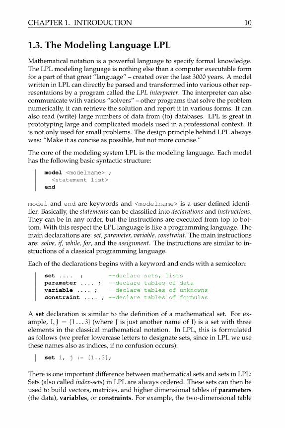
Mathematical notation is a powerful language to specify formal knowledge.The LPL modeling language is nothing else than a computer executable formfor a part of that great “language” – created over the last 3000 years. A modelwritten in LPL can directly be parsed and transformed into various other rep-resentations by a program called the LPL interpreter. The interpreter can alsocommunicate with various “solvers” – other programs that solve the problemnumerically, it can retrieve the solution and report it in various forms. It canalso read (write) large numbers of data from (to) databases. LPL is great inprototyping large and complicated models used in a professional context. Itis not only used for small problems. The design principle behind LPL alwayswas: “Make it as concise as possible, but not more concise.”

The core of the modeling system LPL is the modeling language. Each modelhas the following basic syntactic structure:

model <modelname> ;<statement list>

end

model and end are keywords and <modelname> is a user-defined identi-fier. Basically, the statements can be classified into declarations and instructions.They can be in any order, but the instructions are executed from top to bot-tom. With this respect the LPL language is like a programming language. Themain declarations are: set, parameter, variable, constraint. The main instructionsare: solve, if, while, for, and the assignment. The instructions are similar to in-structions of a classical programming language.

Each of the declarations begins with a keyword and ends with a semicolon:

set .... ; --declare sets, listsparameter .... ; --declare tables of datavariable .... ; --declare tables of unknownsconstraint .... ; --declare tables of formulas

A set declaration is similar to the definition of a mathematical set. For ex-ample, I, J = {1 . . . 3} (where J is just another name of I) is a set with threeelements in the classical mathematical notation. In LPL, this is formulatedas follows (we prefer lowercase letters to designate sets, since in LPL we usethese names also as indices, if no confusion occurs):

set i, j := [1..3];

There is one important difference between mathematical sets and sets in LPL:Sets (also called index-sets) in LPL are always ordered. These sets can then beused to build vectors, matrices, and higher dimensional tables of parameters(the data), variables, or constraints. For example, the two-dimensional table

11 CHAPTER 1. INTRODUCTION

ai,j with i, j ∈ I (that is, a 3× 3 data matrix)

ai,j =

1 2 34 5 67 8 9

can be declared in LPL as follows (the single entries are listed in lexicograph-ical ordering, row by row from left to right, the commas are optional):

parameter a{i,j} := [1 2 3 , 4 5 6 , 7 8 9];

The main difference between the mathematical notation and LPL’s notationis that in LPL we do not need to distinguish between the set names and theindex names. Of course, we could also write:

set I; J; -- set name uppercaseparameter a{i in I,j in J}; -- index names lowercase

to make a difference between set name and index name, but this is not nec-essary in most contexts. A further difference, as already mentioned, betweenmathematical sets and sets defined in LPL is that mathematical sets are un-ordered, while in LPL they are always ordered. However, this difference onlybecomes important when we are referencing, for example, the elements bytheir relative or absolute position, as in expression i − 1 (an expression thatreturns the previous element of element i).

A declaration of a vector of unknown quantities (called variables) is writtenin mathematical notation as xj with j ∈ J. In LPL we write it as follows:

variable x{j};

If the variables are integer or binary we write:

integer variable x{j} [0..100];binary variable y{i};

The expression [0..100] means that the integer variables x{j} are boundto the range [0 . . . 100]. Binary variable can only be zero or one. This means:yi ∈ {0, 1} with i ∈ I.

Constraints are defined in the same way. A constraint vector:2

2The formula uses a very common mathematical symbol (∑

), which is a shortcut fora summation. Hence,∑

j∈J

xj with J = {1 . . . n} is the same as x1 + x2 + . . . + xn

where n is a positive integer. It is supposed that the reader is familiar with thisnotation. In the context of this book and if it is clear to which set the index j is

CHAPTER 1. INTRODUCTION 12

∑j∈J

xj + yi ≤ 10 for all i ∈ I

The constraint is written in LPL as follows:

constraint D{i}: sum{j} x[j] + y[i] <= 10;

In LPL, each constraint has a name (here D) and can be indexed like a variableor a parameter. If the context allows it, the indexes within the expressionscan even be dropped (but this is a matter of style). So the constraint can alsocompactly be written as follows:

constraint D{i}: sum{j} x + y <= 10;

The solve statement is identical to the constraint, except that it begins withthe keyword maximize or minimize. If there is no objective function andwe are only looking for a feasible solution then in LPL we can just use thekeyword solve.

maximize obj: sum{j} x;minimize obj: sum{j} x;solve;

A Simple Example

These basic syntax elements allows us to write complete mathematical modelsin LPL. This is illustrated by a simple example:

Suppose your company produces laptops and printers. A laptop takes 6 hoursof work and generates a revenue of 300=C, while a printer takes 2 hours ofwork and generates a revenue of 200=C. Furthermore, the space in our labo-ratory is limited to 350m2 and each product takes 5m2 of space. We want tofind the “best” production mix, that means, how many of each can be man-ufactured in a week, if the total hours of work is limited to 300 hours perweek?

referring, we also often use the shorter notation∑j

xj instead of∑j∈J

xj with J = {1 . . . n}

In concordance with the LPL syntax, we often do not introduce the symbol for theset J, we just use a index name j. So we use the notation

j ∈ {1 . . . n} instead of j ∈ J , J = {1 . . . n}

13 CHAPTER 1. INTRODUCTION

x

y

6x+2y=300

5x+5y=350

C

A

B

D

Figure 1.1: The Feasible Space

To find the optimal production mix, we introduce two symbols x and y for the(unknown) quantities for the two products. Then the production is limited to6x + 2y ≤ 300 hours, and to 5x + 5y ≤ 350 m2. This is best displayed bya diagram (see Figure 1.1). The points (x, y) within the quadrangle ABCDare the only points that do not violate the two requirements. The point C= (40, 30) is particularly interesting, because it defines the production mixwith the highest revenue, that means, 300x + 200y – the revenue of the mix– cannot be larger without violating either the time or the space constraint.Mathematically we say, that point C maximizes the expression 300x + 200y.We can formulate the problem as a linear system in the following way:

max 300x+ 200ysubject to 6x+ 2y ≤ 300

5x+ 5y ≤ 350x, y ≥ 0

The formulation says to maximize an expression such that the “subject to”conditions (called constraints) are fulfilled. In LPL the problem can be formu-

CHAPTER 1. INTRODUCTION 14

lated as follows (see model tutor013):

model simple;variable x; y;maximize revenue: 300*x + 200*y;constraint A: 6*x + 2*y <= 300;constraint B: 5*x + 5*y <= 350;

end

As expected, solving the model gives x = 40 and y = 30.

The simple example is an instance of an important class of problems having ahuge number of real applications. In the operations research (OR) communitythe class is called linear programs or LP. The general linear model containing nconstraints and m variables can be compactly formulated as follows:

max∑j∈J

cjxj

subject to∑j∈J

Ai,jxj ≤ bi for all i ∈ I

xj ≥ 0 for all j ∈ Jwith J = {1 . . .m}, I = {1 . . . n}, m, n ≥ 0

An even more compact formulation using matrix notation for the model is:

max cxsubject to Ax ≤ b

x ≥ 0

In LPL the general model can be formulated as follows:

model myLP;set i; j;parameter A{i,j}; c{j}; b{i};variable x{j};constraint C{i}: sum{j} A*x <= b;maximize obj: sum{j} c*x;

end

This is very close to the mathematical notation. The model first declares thetwo sets i and j. The data matrix and the two vectors are compactly declaredas Ai,j, cj and bi.4 There size will depend of the number of elements of thetwo sets. The variable vector xj is also declared in a similar way. (The posi-tivity of the variable is automatically assumed by LPL, if no range is given.)

3 http://lpl.virtual-optima.com/lpl/Solver.jsp?name=/tutor014 Note – as already mentioned – in LPL syntax index names can be the same as set

names if no ambiguity is created.

15 CHAPTER 1. INTRODUCTION

The constraints and the maximizing function are also very close to the math-ematical notation. The model does not contain data. They can be added bya separate submodel. For example, to formulate the small example above inthis general form, the data can be added as :

model data;i := [1..2]; j := [1..2];A{i,j} := [6 2 , 5 5];c{j} := [300 200];b{i} := [300 350];

end

Data – we already gave an example – can be placed within the model code orit can be read from files using the Read function. The following data matrix:

ai,j =

2 3 −4 1 15

−5 4 8 1 52 1 14 1 173 4 5 1 70 8 −3 10 1

with i ∈ I, j ∈ J

could be written in LPL as:

set i, j := [1..5];parameter a{i,j} := [2 3 -4 1 15, -5 4 8 1 5,

2 1 14 1 17, 3 4 5 1 7, 0 8 -3 10 1 ];

The matrix elements are listed in lexicographical order (other formats exist).Of course, for large data tables, it is better to read them from files or databasetables. A comma-separated second identifier just introduces another namefor the same set. Hence, i and j represent the same set, but they may be usedas different index names.

Writing the results can be done using the Writep and Write functions. Thesimplest way to output the values of the variable vector x{j} is as follows;

Writep(x);

However, sometimes we need to format the output. To write each value of xjtogether with the set element name on a separate line, we may write in LPL:

Write{j}('Element: %s Value= %6.2f \n', j,x);

The string in single quotes contains the literal text and formatting instructionsthat must be written. %s is a place holder for strings and %6.2f is a placeholder for floating point data (with width 6 and 2 decimals). The values of thefollowing two parameters ,j,x replace the placeholders in the string. Thisexpression means to write (for each element in the set j) on a separate line thefollowing two elements, that is (j,x). More information on this powerful“reporting instruction” can be found in the reference manual of LPL.

CHAPTER 1. INTRODUCTION 16

Data can also be assigned by the assignment instruction. The table assignment

ai,j = cj + bi for all i ∈ I, j ∈ J

would be formulated in LPL as follows:

a{i,j} := c[j] + b[i];

Another often used instruction in the presented case studies is the for loop.Suppose, one would like to optimize a model 10 times (with different param-eters), then one could write:

set loop := [1..10];for{loop} domaximize obj: ... ;....

end

The loop can contain a sequence of any instructions.

The reader should now be able to read and recognize the most basic state-ments of LPL in order to work with the case studies in the following chapters.There is no room here to explain each detail of the language. The interesteduser can get a free LPL version together with the definite language referenceguide and tutor examples. It can be downloaded from the LPL-site.

1.4. Mathematical NotationThe mathematical notation in this book deviates in somewhat from the com-mon notations in three ways.

1.4.1 Set-Names versus Index-Names

The LPL syntax uses some shortcuts in mathematical notation which is re-flected also in the notation of mathematical expressions used in this book. Asalready mentioned, one can use an set name also as an index name and viceversa. So we use the following shorter notation in LPL :

set i := 1..10;set j := 1..5;parameter b{i,j} := i*j;parameter a{i} := sum{j} b[i,j];

instead of the longer notation (although this second notation is also perfectlycorrect in LPL) :

17 CHAPTER 1. INTRODUCTION

set I := 1..10;set J := 1..5;parameter b{i in I,j in J} := i*j;parameter a{i in I} := sum{j in J} b[i,j];

This is also reflected in the mathematical notation often used in this book as :

bi,j = i · j for all i, jai =

∑j

bi,j for all i

i ∈ {1, . . . , 10}j ∈ {1, . . . , 5}

instead of the usual notation :

bi,j = i · j for all i ∈ I, j ∈ J

ai =∑j∈J

bi,j for all i ∈ I

i ∈ I I = {1, . . . , 10}j ∈ J J = {1, . . . , 5}

The difference is that we do not use the set names I or J, if the context is clear,only index names i or j are written.

1.4.2 Logic-mathematical Notation

LPL does not distinguish between Boolean and mathematical operators. AllBoolean operator return 0 or 1, which might be interpreted as false and true.Hence, one can mix these operators in an expression. This is also true inconstraints. We may write, for example:

a=0 or b=1(a=1) + (b=10)

The first expression is common in all kind of programming languages andis a Boolean expression that is true if a is zero or if b is one. The secondexpression seems to be a little bit strange. But on the light that all expressionsare numerical, we have: a = 1 is zero or one, and also b = 10 is zero or one, sothe result of the second expression is zero, one or two. This is also used in themathematical notation and in constraints. For example, in the model will075,the constraint (with variables dm,t ∈ {0, 1} and xm,t ≥ 0) is used:

dm,t ← xm,t > 0

The expression means: “the mine is working if ore is extracted from it”, or “ifa certain positive quantity of ore is delivered from a mine then the variabe dis defined to be true”.

5 http://lpl.virtual-optima.com/lpl/Solver.jsp?name=/will07

CHAPTER 1. INTRODUCTION 18

1.4.3 Logical Operators

LPL uses various logical and Boolean operators that can also be used in con-straints, see Table 1.1. Many problems can be formulated using Boolean orlogical constraints.

Meaning Math. notation LPL syntaxand x∧ y x and yor x∨ y x or ynot ¬x ~xnot and xnandy (¬(x∧ y) x nand ynot or xnory (¬(x∨ y) x nor yimplication x→ y x -> yrev. impl. x← y x <- yexclusive or x ∨̇y x xor yequivalence x ⇐⇒ y x <-> yindexed and

∧i xi and{i} x[i]

indexed or∨

i xi or{i} x[i]indexed xor

∨̇ixi xor{i} x[i]

forall ∀i xi forall{i} x[i]exists ∃i xi exist{i} x[i]indexed nand nandi xi nand{i} x[i]indexed nor nori xi nor{i} x[i]at least 2 atleast(2)i xi atleast(2){i} x[i]at most 2 atmost(2)i xi atmost(2){i} x[i]exactly 2 exactly(2)i xi exactly(2){i} x[i]

Table 1.1: Logical Operators

CHAPTER 2

PROBLEMS FROM WILLIAM’SBOOK

“Approach your problem from the right end and begin with theanswer. Then one day, perhaps you will find the final ques-tion.”

— R. van Gulik

“It isn’t that they can’t see the solution. It is that they can’t seethe problem.”

— G. K. Chesterton

“No mathematician can be a complete mathematician unless heis also something of a poet.”

— Weierstrass

This chapter presents all the models exposed in the famous modeling bookof Williams [29]. All models are implemented in LPL and can be executedstraight away.

19

CHAPTER 2. PROBLEMS FROM WILLIAM’S BOOK 20

2.1. Food Manufacture I (will01)

Problem: A company manufactures (over the next six months) one food by re-fining various raw oils, which come in vegetable and non-vegetable oil – eachwith a given “hardness”. The company can buy oils in the different months.The storage capacity is not a limitation but costs 5ct/ton. The refining capac-ity, however, is limited at 200 tons of veg oil and 250 tons of non-veg oils. The“hardness” of the food must be in certain given ranges. How many tons ofeach oil should the company buy, store, and use in each period in order tomaximize profit by selling the food at a given price ?

Model: The Model is as follows:The problem is from [29] Chapter 13.1.

Listing 2.1: The Complete Model in LPL [15]� �model Will01 "Food Manufacture I";set p := [ January February March April May June ];

r := [ VEG1 VEG2 OIL1 OIL2 OIL3 ] "all oils";v{r} := [ VEG1 VEG2 ] "veg oils";

parameter pr{p,r} := [110 120 130 110 115, 130 130 110 90 115110 140 130 100 95, 120 110 120 120 125100 120 150 110 105, 90 100 140 80 135 ];

hardness{r} := [ 8.8 6.1 2.0 4.2 5.0 ];Pr:=150; Sto:=500; vegCapa:=200; oilCapa:=250;

variablefood{p} "Quantity of food produced";buy{p,r} "Quantity bought in each period";use{p,r} "Quantity used in each period";sto{p,r} "Quantity stored in each period";

constraintBal{r,p}: if(p=1,Sto,sto[p-1,r]) + buy = use + sto;Endstore{r}: sto[#p,r] = Sto;Capacity1{p}: sum{v} use <= vegCapa;Capacity2{p}: sum{r|~v} use <= oilCapa;Hardness{p}: 3*food <= sum{r} hardness*use <= 6*food;Conserve{p}: sum{r} use = food;

maximize profit: sum{p}Pr*food - sum{p,r}(pr*buy+5*sto);Writep(profit,buy,use,sto,food);end� �

21 CHAPTER 2. PROBLEMS FROM WILLIAM’S BOOK

2.2. Food Manufacture II (will02)

Problem: A company manufactures (over the next six months) one food by re-fining various raw oils, which come in vegetable and non-vegetable oil – eachwith a given “hardness”. The company can buy oils in the different months.The storage capacity is not a limitation but costs 5ct/ton. The refining capac-ity, however, is limited at 200 tons of veg oil and 250 tons of non-veg oils. The“hardness” of the food must be in certain given ranges. How many tons ofeach oil should the company buy, store, and use in each period in order tomaximize profit by selling the food at a given price ? Furthermore, we wishto impose the following restrictions :

1. The food may never be made up of more than three different oils.

2. If an oil is used at least 20 tons must be used.

3. If either vegetable oil Veg1 or Veg2 is used, then non-vegetable oilOil3 must also be used.

Model: The Model is as follows:The problem is from [29] Chapter 12.2. Themodel is the same as will011, with exception of the additional restrictions. toimpose these conditions we introduce a 0-1 variable d which is 1 only if thequnatity used (use) of an oil is not zero, that is we must impose:

use > 0↔ d = 1

Listing 2.2: The Complete Model in LPL [15]� �model Will02 "Food Manufacture II";set p := [ January February March April May June ];

r := [ VEG1 VEG2 OIL1 OIL2 OIL3 ] "all oils";v{r} := [ VEG1 VEG2 ] "veg oils";

parameter pr{p,r} := [110 120 130 110 115, 130 130 110 90 115110 140 130 100 95, 120 110 120 120 125100 120 150 110 105, 90 100 140 80 135 ];

hardness{r} := [ 8.8 6.1 2.0 4.2 5.0 ];Pr:=150; Sto:=500; vegCapa:=200; oilCapa:=250;

variablefood{p} "quantity of food produced";buy{p,r} "quantity bought in each period";use{p,r} "quantity used in each period";sto{p,r} "quantity stored in each period";binary d{p,r}; // is 1 if use>0

constraint

1 http://lpl.virtual-optima.com/lpl/Solver.jsp?name=/will01

CHAPTER 2. PROBLEMS FROM WILLIAM’S BOOK 22

Bal{r,p}: if(p=1,Sto,sto[p-1,r])+buy = use+sto;endstore{r}: sto[#p,r]=Sto;Capacity1{p}: sum{v} use <= 200;Capacity2{p}: sum{r|~v} use <= 250;Hardness{p}: 3*food <= sum{r} hardness*use <= 6*food;Conserve{p}: sum{r} use = food;Cond1{p}: sum{r} d <= 3;Cond2{p,r} :use-20*d >=0; -- use>0 -> d=1Cond2a{p,r}:use-if(v,200,250)*d <=0; -- d=1 -> use>0Cond3{p}: d[p,'VEG1']+d[p,'VEG2']-2*d[p,'OIL3']<=0;

maximize profit: sum{p}Pr*food - sum{p,r}(pr*buy+5*sto);Writep(profit,buy,use,sto,food);end� �

23 CHAPTER 2. PROBLEMS FROM WILLIAM’S BOOK

2.3. Factory planning I (will03)

Problem: Seven products are manufactured using different machines over thenext month. Each product yields a certain contribution to profit. Several ma-chines will be down in different months for maintenance. We also want agiven endstock for each product at the end of our time horizont. What mustbe manufactured, stored and sold each month in order to maximize profit, ifthe storage is limited and the market also has limitations on each product?

Model: The Model is as follows:The problem is from [29] Chapter 13.3.

Listing 2.3: The Complete Model in LPL [15]� �model Will03 "Factory planning I";set

p:=[Prod1 Prod2 Prod3 Prod4 Prod5 Prod6 Prod7] "prod";m:=[grinder vDrill hDrill borer planer] "mach";t:=[Jan Feb Mar Apr May Jun] "period";

parameter profit{p} := [10 6 8 4 11 9 3];time{m,p} "machine time table" :=[.5 .7 . . .3 .2 .5,.1 .2 . .3 . .6 . , .2 . .8 . . . .6 ,.05 .03 . .07 .1 . .08 , . . .01 . .05 . .05];

down{t,m} "number of machines down" := [(Jan,grinder) 1 (Feb,hDrill) 2 (Mar,borer) 1(Apr,vDrill) 1 (May,grinder) 1 (May,vDrill) 1(Jun,planer) 1 (Jun,hDrill) 1];

qMach{m} "nr. of machines available" := [4 2 3 1 1];upper{t,p} "market limitation of sells" := [500 1000300 300 800 200 100, 600 500 200 0 400 300 150, 300600 0 0 500 400 100, 200 300 400 500 200 0 100, 0100 500 100 1000 300 0, 500 500 100 300 1100 500 60];

storeCost := 0.5; storeCapacity := 100;endStock := 50; hoursMonth := 2*8*24;

variablemanu{t,p} "quantity manufactured";held{t,p} "quantity stored";sell{t,p} [0..upper] "quantity sold";

constraintBalance{t,p}: held[t-1,p] + manu = sell + held;endstore{p}: held[#t,p] = endStock;storecapa{t,p|t<#t}: held <= storeCapacity;capa{t,m}: sum{p} time*manu <= hoursMonth*(qMach-down);

maximize Profit: sum{t,p} (profit*sell - storeCost*held);Writep(Profit,manu,held,sell);Write(' Manufacture Sell Store\n');Write{t,p}('%5s %5s %8d %8d %8d\n',t,p,manu,sell,held);end� �

CHAPTER 2. PROBLEMS FROM WILLIAM’S BOOK 24

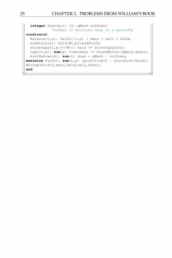
2.4. Factory planning II (will04)

Problem: Seven products are manufactured using different machines over thenext month. Each product yields a certain contribution to profit. Several ma-chines will be down in different months for maintenance. We also want agiven endstock for each product at the end of our time horizont. What mustbe manufactured, stored and sold each month in order to maximize profit, ifthe storage is limited and the market also has limitations on each product?Instead of stipulating when each machine is down, it is desired to find thebest month for each machine to be down. Each machine must be down oncein the six months except two grinders.

Model: The Model is as follows:The problem is from [29]. For a problem de-scription see Chapter 13.4. Note that this is the same model as will032 exceptthat down is now a variable.

Listing 2.4: The Complete Model in LPL [15]� �model Will04 "Factory planning II";set

p:=[Prod1 Prod2 Prod3 Prod4 Prod5 Prod6 Prod7] "prod";m:=[grinder vertDrill horiDrill borer planer] "mach";t:=[January February March April May June] "period";

parameterprofit{p} "profit per p" := [ 10 6 8 4 11 9 3 ];time{m,p} "machine time table" := [

0.5 0.7 . . 0.3 0.2 0.50.1 0.2 . 0.3 . 0.6 .0.2 . 0.8 . . . 0.60.05 0.03 . 0.07 0.1 . 0.08. . 0.01 . 0.05 . 0.05 ];

qMach{m} "nr of machines" := [ 4 2 3 1 1];notDown{m} "nr not-down" := [ 2 . . . .];upper{t,p} "market limitation of sells" := [

500 1000 300 300 800 200 100600 500 200 0 400 300 150300 600 0 0 500 400 100200 300 400 500 200 0 100

0 100 500 100 1000 300 0500 500 100 300 1100 500 60 ];

storeCost := 0.5; storeCapacity := 100;endStock := 50; hoursMonth := 2*8*24;

variablemanu{t,p} "quantity manufactured";held{t,p} "quantity stored";sell{t,p} [0..upper] "quantity sold";

2 http://lpl.virtual-optima.com/lpl/Solver.jsp?name=/will03

25 CHAPTER 2. PROBLEMS FROM WILLIAM’S BOOK

integer down{m,t} [0..qMach-notDown]"number of machines down in a period";

constraintBalance{t,p}: held[t-1,p] + manu = sell + held;endstore{p}: held[#t,p]=endStock;storecapa{t,p|t<>#t}: held <= storeCapacity;capa{t,m}: sum{p} time*manu <= hoursMonth*(qMach-down);mustBeDown{m}: sum{t} down = qMach - notDown;

maximize Profit: sum{t,p} (profit*sell - storeCost*held);Writep(Profit,manu,held,sell,down);end� �

CHAPTER 2. PROBLEMS FROM WILLIAM’S BOOK 26

2.5. Manpower Planning (will05)

Problem: A company is undergoing a number of changes over the next 3 yearswhich will affect its manpower requirements in future years. “Less unskilled”and “more skilled” men are needed. It also has “semi-skilled”. The companymust decide its policy with regard the following:

1. Recruitment from outside the company which is limited

2. Retraining from less skilled to more skilled

3. Redundancy and overmanning which causes extra costs and

4. Short-time working

The company declared to minimize the overall redundancy and costs.

Model: The Model is as follows:The problem is from [29]. For a problemdescription see Chapter 13.5.

Listing 2.5: The Complete Model in LPL [15]� �model Will05 "Manpower Planning";

set year,y := [1..3];skill,s,t := [Unskilled,SemiSkilled,Skilled];

parameterCurrentStrength{s} := [2000,1500,1000];Requirement{y,s} := [1000, 1400, 1000,

500, 2000, 1500, 0, 2500, 2000];LeaveFirstYear{s} := [0.25, 0.20, 0.10];LeaveEachYear{s} := [0.10, 0.05, 0.05];ContinueFirstYear{s} := 1-LeaveFirstYear;ContinueEachYear{s} := 1-LeaveEachYear;LeaveDownGraded := 0.50;ContinueDownGraded := 1-LeaveDownGraded;MaxRecruit{s} := [500, 800, 500];MaxRetrainUnskilled := 200;MaxOverManning := 150;MaxShortTimeWorking := 50;RetrainSemiSkilled := 0.25;ShortTimeUsage := 0.50;RetrainCost{s} := [400, 500, 0];RedundantCost{s} := [200, 500, 500];ShortTimeCost{s} := [500, 400, 400];OverManningCost{s} := [1500, 2000, 3000];

variableLaborForce,L{s,y};Recruite, R{s,y} [0..MaxRecruit];Retrain, T{s,t,y};

27 CHAPTER 2. PROBLEMS FROM WILLIAM’S BOOK

Redundant, D{s,y};ShortTime, S{s,y} [0..MaxShortTimeWorking];OverManned,O{s,y};

expressionTotalRetrainCost : sum{y,s} RetrainCost*T[s,s+1,y];TotalRedundantCost : sum{s,y} RedundantCost*D;TotalShortTimeCost : sum{s,y} ShortTimeCost*S;TotalOverManningCost: sum{s,y} OverManningCost*O;TotalManpowerCost:TotalRetrainCost+TotalRedundantCost+TotalOverManningCost + TotalShortTimeCost;

TotalRedundantMen : sum{s,y} D;constraintContinuity{s,y}: L =

ContinueEachYear*if(y=1,CurrentStrength,L[s,y-1])+ ContinueFirstYear*R + 0.95*T[s-1,s,y]+ sum{t} ContinueDownGraded*T[s+t,s,y]- sum{t} T[s,s-t,y] - T[s,s+1,y] - D;

RetainMaxUnskilled{y}:T['Unskilled','SemiSkilled',y]<=200;

RetrainingSemiSkilled{y}: T['SemiSkilled','Skilled',y]<= RetrainSemiSkilled*L['Skilled',y];

OverManning{y}: sum{s} O <= MaxOverManning;Requirements{s,y}: L = Requirement+O+ShortTimeUsage*S;minimize TotalRedundancy: TotalRedundantMen;Writep(TotalManpowerCost,TotalRedundantMen,

Recruite,Retrain,ShortTime,OverManned);end� �

CHAPTER 2. PROBLEMS FROM WILLIAM’S BOOK 28

2.6. Refinery Optimization I (will06)

Problem: An oil refinery purchases two crude oil, which are subject to fourprocesses:

1. Distillation which yields light, medium, and heavy naphtha as well aslight oil, heavy oil, and residuum

2. Reforming which yields reformed gasoline using the naphthas.

3. Cracking which yields cracked oil and gasoline using the oils

4. Blending which yields the final products: regular and premium petrol,jet fuel, fuel oil, and lube oil. The objective is to maximize profit.

Model: The Model is as follows:The problem is from [29]. For a problemdescription see Chapter 13.6.

Listing 2.6: The Complete Model in LPL [15]� �model Will06 "Refinery Optimization I";

set c := [Crude1, Crude2];f := [LightNaphtha MediumNaphtha HeavyNaphtha

LightOil HeavyOil Residuum];n{f} := [LightNaphtha MediumNaphtha HeavyNaphtha];o{f} := [LightOil HeavyOil];a := [CrackedOil CrackedGasoline];p:=[PremiumFuel RegularFuel JetFuel FuelOil LubeOil];m{p} := [PremiumFuel, RegularFuel];

parameterDistillYld{c,f}:=[0.10 0.20 0.20 0.12 0.20 0.13,

0.15 0.25 0.18 0.08 0.19 0.12];ReformingYield{n} := [0.60, 0.52, 0.45];CrackingYield{o,a} := [0.68, 0.28, 0.75, 0.20];ResiduumLubeOilYield := 0.50;VaporPressure{o} := [1.0, 0.6];VaporPressureCrackedOil := 1.5;VaporPressureResiduum := 0.05;FuelOilRatio{o} := [.55555, .16666];FuelOilRatioCrackedOil := 4/18;FuelOilRatioResiduum := 1/18;OctaneNumberNaphtha{n} := [90, 80, 70];OctaneNumberReformedGas := 115;OctaneNumberCrackedGas := 105;MinOctaneLevel{m} := [94, 84];CrudeDailyAvail{c} := [20000, 30000];DistillCapacity := 45000;ReformingCapacity := 10000;CrackingCapacity := 8000;

29 CHAPTER 2. PROBLEMS FROM WILLIAM’S BOOK

MinLubeOil := 500;MaxLubeOil := 1000;MinPremiumProdPct := 0.40;Profit{p} := [7.00 6.00 4.00 3.50 1.50];

variableFinalProduct{p}; PurchaseCrude{c};DistillOutput{f}; NaphthaForReformGas{n};ReformedGasoline; OilForCracking{o};CrackedOutput{a}; NaphthaForMotorFuel{n,m};ReformedGasForMotorFuel{m};CrackedGasForMotorFuel{m};OilForJetFuel{o}; ResiduumForJetFuel;CrackOilForJetFuel; ResiduumForLubeOil;

maximize TotalProfit: sum{p} Profit*FinalProduct;constraintDistillLimit "At most 45000 barrels of crude can be

distilled per day":sum{c} PurchaseCrude <= DistillCapacity;

ReformingLimit "At most 10000 barrels of naphtha canbe reformed per day":sum{n} NaphthaForReformGas <= ReformingCapacity;

CrackingLimit "At most 8000 barrels of oil can becracked per day":sum{o} OilForCracking <= CrackingCapacity;

DistillationBalance{f} "Balance crude inputs todistillation outputs":sum{c} DistillYld*PurchaseCrude = DistillOutput;

ReformedGasBalance "Balance naphtha inputs toreformed gas output":sum{n} ReformingYield*NaphthaForReformGas =

ReformedGasoline;CrackBalance{a} "Balance oil inputs to cracked output

":sum{o} CrackingYield*OilForCracking =

CrackedOutput;ResiduumLubeOil "Each barrel of residuum yields 0.5

barrels of lube oil":ResiduumLubeOilYield*ResiduumForLubeOil =

FinalProduct['LubeOil'];DivideReformGas "Divide reformed gas to motor fuels":

ReformedGasoline = sum{m}ReformedGasForMotorFuel;DivideNaphtha{n} "Divide naphthas to reformed gas and

motor fuels":DistillOutput = NaphthaForReformGas + sum{m}

NaphthaForMotorFuel;DivideOil{o} "Divide light/heavy oils to cracking,

jet fuel, and fuel oil":DistillOutput = OilForCracking + OilForJetFuel +

FuelOilRatio*FinalProduct['FuelOil'];DivideCrackGas "Divide cracked gasoline to motor

CHAPTER 2. PROBLEMS FROM WILLIAM’S BOOK 30

fuels":CrackedOutput['CrackedGasoline'] = sum{m}

CrackedGasForMotorFuel;DivideCrackedOil "Divide cracked oil to jet fuel and

fuel oil":CrackedOutput['CrackedOil'] = CrackOilForJetFuel+ FuelOilRatioCrackedOil*FinalProduct['FuelOil'];

DivideResiduum "Divide Residuum to jet fuel, fuel oil, and lube oil":DistillOutput['Residuum'] = ResiduumForJetFuel+ FuelOilRatioResiduum*FinalProduct['FuelOil'] +

ResiduumForLubeOil;BlendMotorFuel{m} "Blending motor fuels from naphtha,

reformed gas, and cracked gas":FinalProduct = sum{n} NaphthaForMotorFuel +

ReformedGasForMotorFuel +CrackedGasForMotorFuel;

BlendJetFuel "Blending jet fuel from light/heavy oils, cracked oil and residuum":FinalProduct['JetFuel'] = sum{o} OilForJetFuel +

CrackOilForJetFuel + ResiduumForJetFuel;MaxVaporPressure "Jet fuel maximum vapor pressure":

sum{o} VaporPressure*OilForJetFuel +VaporPressureCrackedOil*CrackOilForJetFuel

+ VaporPressureResiduum*ResiduumForJetFuel <=FinalProduct['JetFuel'];

MinPremFuel "Premium fuel at least 40% of Regular":FinalProduct['PremiumFuel'] >= MinPremiumProdPct*

FinalProduct['RegularFuel'];MinOctFuel{m} "Motor fuels minimum octane levels":

sum{n} OctaneNumberNaphtha*NaphthaForMotorFuel+ OctaneNumberReformedGas*ReformedGasForMotorFuel+ OctaneNumberCrackedGas*CrackedGasForMotorFuel>= MinOctaneLevel*FinalProduct;

C{c}: PurchaseCrude <= CrudeDailyAvail;D: MinLubeOil<= FinalProduct['LubeOil'] <=MaxLubeOil;

Writep(TotalProfit);SetFocus(); //write all variableswhile NextFocus(3) dowhile NextPosition() do

Write('%-47s %d\n', GetName(0), GetValue(0));end;

endend� �

31 CHAPTER 2. PROBLEMS FROM WILLIAM’S BOOK

2.7. Refinery Optimization II (will06a)

Problem: An oil refinery purchases two crude oil, which are subject to fourprocesses:

1. Distillation which yields light, medium, and heavy naphtha as well aslight oil, heavy oil, and residuum

2. Reforming which yields reformed gasoline using the naphthas.

3. Cracking which yields cracked oil and gasoline using the oils

4. Blending which yields the final products: regular and premium petrol,jet fuel, fuel oil, and lube oil. The objective is to maximize profit.

Model: The Model is as follows:The problem is from [29]. For a problemdescription see Chapter 13.6.

Listing 2.7: The Complete Model in LPL [15]� �model Will06a "Refinery Optimization II";variable

cr1; cr2; ln; mn; hn; lo; ho; r; lnrg; mnrg; hnrg; rg;locgo; hocgo; cg; co; lnpmf; lnrmf; mnpmf; mnrmf;hnpmf;hnrmf; rgpmf; rgrmf; cgpmf; cgrmf; lojf; hojf; rjf;cojf; lofo; hofo; rfo; cofo; rlbo; pmf; rmf;jf; fo; lbo;

constraintr1: cr1 <= 20000; --availabilitiesr2: cr2 <= 30000;r3: cr1+cr2 <= 45000; --capacityr4: lnrg+mnrg+hnrg <= 10000; --reforming capacityr5: locgo+hocgo <= 8000; --cracking capacityr6: 500 <= lbo <= 1000; --boundsr8: 0.1 *cr1 +0.15*cr2 >= ln; --split under

destillationr9: +0.2 *cr1 +0.25*cr2 >= mn;r10: +0.2 *cr1 +0.18*cr2 >= hn;r11: +0.12*cr1 +0.08*cr2 >= lo;r12: +0.2 *cr1 +0.19*cr2 >= ho;r13: +0.13*cr1 +0.12*cr2 >= r;r14: +0.6*lnrg+0.52*mnrg+0.45*hnrg >= rg; --splitting

under reformingr15: 0.68*locgo+0.75*hocgo = co; --splitting under

crackingr16: 0.28*locgo+0.2 *hocgo = cg;r17: lnrg+lnpmf+lnrmf = ln; --continuitiesr18: mnrg+mnpmf+mnrmf = mn;r19: hnrg+hnpmf+hnrmf = hn;

CHAPTER 2. PROBLEMS FROM WILLIAM’S BOOK 32

r20: locgo+lojf+0.55*fo = lo; --fixed proportions onfuel oil in blending

r21: hocgo+hojf+0.17*fo = ho;r22: cojf+0.22*fo = co;r23: rlbo+rjf+0.055*fo = r;r24: cgpmf+cgrmf = cg; --further continuitiesr25: rgrmf+rgpmf = rg;r26: +lnpmf+mnpmf+hnpmf+rgpmf+cgpmf = pmf;r27: +lnrmf+mnrmf+hnrmf+rgrmf+cgrmf = rmf;r28: +lojf+hojf+cojf+rjf = jf;r29: +0.5*rlbo = lbo; --lube-oil is 0.5 of residuum

usedr30: pmf >= 0.4*rmf; --pmf/rmf must be 40%r31: +90*lnpmf+80*mnpmf+70*hnpmf+115*rgpmf+105*cgpmf >=

94*pmf; --octane numberr32: +90*lnrmf+80*mnrmf+70*hnrmf+115*rgrmf+105*cgrmf >=

84*rmf;r33: +lojf+0.6*hojf+1.5*cojf+0.05*rjf <= jf; --

vapour pessure constraintsmaximize profit: 7*pmf+6*rmf+4*jf+3.5*fo+1.5*lbo;

Writep(profit);while NextFocus(3) dowhile NextPosition() do

Write('%-10s %d\n', GetName(0), GetValue(0));end;

endend� �

33 CHAPTER 2. PROBLEMS FROM WILLIAM’S BOOK

2.8. Mining (will07)

Problem: A mining company extracts ore from several mines over the nextfive years. The ore from different mines is of varying quality and the extractedamount of ore is limited. Furthermore, royalities are payable on each minekept open. The company can operate on three of the four available mines ata time. A mine can be closed and no royalities are payable. A closed mine,however, must be closed down permanently. Which mines should be oper-ated each period and how much should they produce? Future revenue andexpentiture must be discounted.

Model: The Model is as follows:The problem is from [29]. For a problemdescription see Chapter 13.7.

Listing 2.8: The Complete Model in LPL [15]� �model Will07 "Mining";set m := [Mine1 Mine2 Mine3 Mine4];

t,t0 := [Year1 Year2 Year3 Year4 Year5];parameter

Royalities{m} := [5 4 4 5];ExtractLimit{m}:= [2 2.5 1.3 3];OreQuality{m} := [1 .7 1.5 .5];BlendedQuality{t} := [0.9 0.8 1.2 0.6 1.0];rate := 10/100;sellPrice := 10;discountFactor{t} := 1/(prod{t0|t0<t} (1+rate));

variablex{m,t}[0..ExtractLimit] "output";q{t} "quantity of blended ore";binary d{m,t} "mine is working (if x>0)";binary g{m,t} "mine is open";

constraintWorkingMines{t}: atmost(3){m} d;NoWorkOnClosedMines{m,t}: d -> g;SubsequentYearsClosed{m,t|t<#t}: g[m,t+1] -> g;Blending{t}: sum{m} OreQuality*x = BlendedQuality*q;Combine{t}: sum{m} x = q;Working{m,t}: d <- x>0 "mine is working if x>0";

maximize profit: - (sum{m,t} discountFactor*Royalities*g)+ sum{t} discountFactor*sellPrice*q;

Writep(profit,x,q,discountFactor,d,g);end� �

CHAPTER 2. PROBLEMS FROM WILLIAM’S BOOK 34

2.9. Farm Planning (will08)

Problem: A farmer wishes to plan production on his farm for the next fiveyears. He has heifers and milk-producing cows. They consume grain andsugar beet which can be grown both on the farm or bought (or sell) on themarket. Heifers produce calves which can be sold (the bollocks are soldimmediately) or which will become milk-producing cows in the third year.Labour can be recruited from outside and extra capital is also available tosome extent. How should the farmer operate to maximize profit over the fiveyears? How much grain and sugar beet should he plant, sell or buy; howmuch extra labour and capital should he use; and how many cows does hehave in each year and of each age?

Model: The Model is as follows:The problem is from [29]. For a problemdescription see Chapter 13.8.

Listing 2.9: The Complete Model in LPL [15]� �model Will08 "Farm Planning";set t,k := [ Year1 Year2 Yera3 Year4 Year5 ];

i := [ 1 2 3 4 ]; /*land groups*/j := [ 1 2 3 4 5 6 7 8 9 10 11 12 ]; --cow agej1{j} := [ 2 3 4 5 6 7 8 9 10 11 ];

parameterGrainYld{i} "grain growing" := [1.1 0.9 0.8 0.65];GrainArea{i} "area in arces" := [ 20 30 20 10];

variableGR{i,t} "grain grown in tons";SB{t} "sugar beet grown in tons";GRBUY{t} "bought grain in tons";GRSELL{t} "sold grain in tons";SBBUY{t} "bought sugar beet in tons";SBSELL{t} "sold sugar beet in tons";EXLAB{t} "extra labour recruited";EXCAP{t} "capital outlay";HFSELL{t} "number of heifers sold at birth";COWS{j,t} "number of cows of age j in year t";NEWCOW{t} "number of cows of age 0 at year t";PROF{t} "profit in year t";

constraintACCOMM{t} "Accommodation (housing capacity)":NEWCOW + sum{j|j<#j} COWS <= 130 + sum{k|k<=t} EXCAP;

GRCONS{t} "Grain consumption":sum{j1} 0.6*COWS[j1,t] <= sum{i} GR + GRBUY - GRSELL;

SBCONS{t} "Sugar beet consumption":sum{j1} 0.7*COWS[j1,t] <= SB + SBBUY - SBSELL;

BOUNDS{i,t} "Grain growing 'capacity'":

35 CHAPTER 2. PROBLEMS FROM WILLIAM’S BOOK

GR <= GrainYld*GrainArea;ACREAS{t} "Acreage limitation":sum{i} 1/GrainYld*GR + 2/3*SB + 2/3*NEWCOW+ 2/3*COWS[1,t] + sum{j1} COWS[j1,t] <= 200;

LABOUR{t} "Labour in 100 hours":0.1*NEWCOW + 0.1*COWS[1,t] + sum{j1} 0.42*COWS[j1,t]+ sum{i} 0.04/GrainYld*GR + 0.14/1.5*SB <= 55+EXLAB;

-- continuity constraintsCTA{t|t<#t}: COWS[1,t+1] = 0.95*NEWCOW[t];CTB{t|t<#t}: COWS[2,t+1] = 0.95*COWS[1,t];CT{j1,t|t<#t}:COWS[j1+1,t+1] = 0.98*COWS[j1,t];CTC{t}: NEWCOW - sum{j1} 0.55*COWS[j1,t] + HFSELL = 0;ENDT "Cows at the end": 50<= sum{j1} COWS[j1,5] <=175;PROFIT{t}:sum{j1} 16.5*COWS[j1,t] + 40*HFSELL + 120*COWS[12,t]+ sum{j1} 370*COWS[j1,t] + 75*GRSELL + 58*SBSELL- 90*GRBUY - 70*SBBUY - 120*EXLAB - 50*NEWCOW- 50*COWS[1,t] - sum{j1} 100*COWS[j1,t]- sum{i}15/GrainYld*GR - 20/3*SB - sum{t}39.71*EXCAP- PROF = 4000;

-- initial conditions, fixing number of cows of eachage at first period

BOUNDS1{j}: COWS[j,1] = if(j<3 , 9.5 , 9.8);-- maximize profit minus discounted capital expendituresmaximize TProf: sum{t} (PROF-158.85*EXCAP-39.71*t*EXCAP);Writep(TProf,GR,SB,GRBUY,GRSELL,SBBUY,SBSELL,EXLAB,

EXCAP,HFSELL,COWS,NEWCOW,PROF);end� �

CHAPTER 2. PROBLEMS FROM WILLIAM’S BOOK 36

2.10. Economic Planning (will09)

Problem: An economy consists of the three industries coal, steel, and trans-port. Each industry requires inputs from its own, inputs from the other indus-tries, and manpower. Output may also be used to build productive capacity,which become effective two periods later. Manpower capacity is limited andan initial stock and productive capacity is given. We wanted to know thegrowth patterns for the economy pursuing the following objectives:

1. Maximizing the productive capacity at the end of the considered timewhile meeting an exogenous demand

2. Maximizing total production the the last two periods ignoring the ex-ogenous demand (set to zero)

3. Maximizing the total manpower requirement ignoring the manpowercapacity limitation while meeting the exogenous demand.

Model: The Model is as follows:The problem is from [29]. For a problemdescription see Chapter 13.9.

Listing 2.10: The Complete Model in LPL [15]� �model Will09 "Economic Planning";

set o,o1 := [Coal Steel Transport] "activities";t,t1 := [1..6] "periods";

parameterreq{o1,o} := [.1 .5 .4 , .1 .1 .2 , .2 .1 .2];cap{o1,o} := [.0 .7 .9 , .1 .1 .2 , .2 .1 .2];Mreq{o} := [.6 .3 .2];Mcap{o} := [.4 .2 .1];Stocks{o} := [ 150 80 100 ] "initial stock" ;Capa {o} := [ 300 350 280 ] "capa. in period 0";consum{o} := [ 60 60 30 ] "exo. demand";consum1{o}:= consum "make a copy of consum";lastx {o} := [166.4 105.7 92.3] "min. end output";manCapa := 470 "labour capacity";

variablex{o,t} [if(t=#t,lastx,0)..99999] "outputs in t";s{o,t} "stock level at beginning of t";y{o,t|t<#t-1} "extra productive capacity for t+1";

constraintTotOutput{o1,t}: sum{o} (req*x+cap*y) + s <=

x[o1,t-1] + s[o1,t-1] + if(t=1,Stocks,-consum);Manpower{t}: sum{o} (Mreq*x+Mcap*y) <= manCapa;prodCapa{o,t|t>1}: x - sum{t1|t1<t} y <= Capa;

maximize obj: sum{o} Capa + sum{o,t} y[o,t];Write('-- (1) maximize the productive capacity\n');

37 CHAPTER 2. PROBLEMS FROM WILLIAM’S BOOK

Writep(obj,y,x,s);consum{o}:=0; /*ignore the exogenous demand*/maximize obj1: sum{o,t|t>=#t-1} x[o,t];Write('-- (2) maximize the final output\n');Writep(obj1,y,x,s);consum{o}:=consum1; /*recopy the original consum*/maximize obj2: sum{t,o} (Mreq*x[o,t+1] + Mcap*y[o,t+2])subject_to (Will09, ~Manpower);

Write('-- (3) maximize the manpower requirement\n');Writep(obj2,y,x,s);

end� �

CHAPTER 2. PROBLEMS FROM WILLIAM’S BOOK 38

2.11. Decentralization (will10)

Problem: A large company wants to move 5 of its departments out of London(to Bristol or Brighton). There are benefits (cheaper housing etc.) and costs(communication) to be derived from doing this. Where should each depart-ment be located so as to minimize overall yearly costs?

Model: The Model is as follows:The problem is from [29]. For a problemdescription see Chapter 13.10.

Listing 2.11: The Complete Model in LPL [15]� �model Will10 "Decentralization";set D,i,k := [A B C D E] "Departements";

C,j,l := [Bristol Brighton London] "Cities";parameter

Benefit{D,C}:=[10 10 0 15 20 0 10 15 0 20 15 0 5 15 0];Cost{C,C}:= [5 14 13, 14 5 9, 13 9 10] "Comm. costs";Comm{D,D}:=[(A,C) 1.0, (A,D) 1.5, (B,C) 1.4, (B,D) 1.2,

(C,E) 2.0, (D,E) 0.7] "quant. of communications";set CO{i,j,k,l} := k>i and Comm[i,k];binary variable

d{D,C} "departement d is in city c";g{CO}; -- g[CO[i,j,k,l] <-> d[i,j] and d[k,l];

constraint-- each department must be located in exactly one cityDept{D}: sum{C} d = 1;-- at most 3 departments be located in the same cityCity{C}: atmost(3){D} d;La{CO[i,j,k,l]}: (g[CO]->d[i,j]) and (g[CO]->d[k,l]);Lc{CO[i,j,k,l]}: d[i,j] and d[k,l] -> g[CO];

minimize TCOST: -(sum{D,C|C<>'London'} Benefit*d)+ sum{CO[i,j,k,l]} Comm[i,k]*Cost[j,l]*g[CO];

Write('Total communication cost %d\n\n', -1000*TCOST);Write{C|exist{D} d}('Locate departements %2s in %s\n',

{D|d} D , C);end� �

This problem is a quadratic assignment problem and objective function in factwould be:

minimize TCOST: -(sum(D,C|C<>'London') Benefit*d+sum([i,j,k,l]=CO) Comm[i,k]*Cost[j,l]*d[i,k]*d[j,l];

To solve this with a standard linear solver, it is possible to reformulate themodel as a linear integer program by the following steps

1. replace xy by a new 0-1 variable z (x and y are also 0-1 variables)

39 CHAPTER 2. PROBLEMS FROM WILLIAM’S BOOK

2. impose the logical condition: z = 1 ↔ x = 1 ∧ y = 1 by means of thethree constraints: z− x ≤ 0 , z− y ≤ 0 , x+ y− z ≤ 1.

An alternative is the objective in the model code together with the two con-straints La and Lb .

CHAPTER 2. PROBLEMS FROM WILLIAM’S BOOK 40

2.12. Curve Fitting (linear) (will11)

Problem: Two quantities x and y are known to be correlated by a straight liney = ax+ b. A number of corresponding values are known.

1. Find a straight line, such that the sum of absolute deviation of all cor-responding values are minimized.

2. Find a straight line, such that the maximum deviation is minimized.

(Note that the standard way to model this is by regression and we minimizethe sum of the quadratic deviations. In this approach different measures of“deviations” are used.)

Modeling Steps

The problem is from [29]. For a problem description see Chapter 13.11.

Define the data: A set I of points (x, y) is given. Model this be two vectors xiand yi, for each point i ∈ I.

1. The goal is to find a linear function: y = Ax + B where A and B areunknown.

2. For each given point, we introduce a unknown positive P and negativeN deviation from the line y = Ax + B. Hence, the following conditionmust hold:

yi = Axi + B+ Pi −Ni for all i ∈ I

3. In a first round we minimize the sum of all deviations, that is:

min∑i

(Pi +Ni)

4. To minimize the maximal deviation, we introduce a new variable maxdevand add the conditions maxdev ≥ Pi and maxdev ≥ Ni for all pointsi. Now maxdev is larger than any Pi or Ni, that means it defines themaximal deviation. Finally, we minimize maxdev.

Listing 2.12: The Complete Model in LPL [15]� �model Will11 "Curve Fitting (linear)";

set i := 1..19; -- 19 points are knownparameterx{i}:=[0.0 0.5 1.0 1.5 1.9 2.5 3.0 3.5 4.0 4.5

5.0 5.5 6.0 6.6 7.0 7.6 8.5 9.0 10.0];y{i}:=[1.0 0.9 0.7 1.5 2.0 2.4 3.2 2.0 2.7 3.5,

41 CHAPTER 2. PROBLEMS FROM WILLIAM’S BOOK

1.0 4.0 3.6 2.7 5.7 4.6 6.0 6.8 7.3];variableA [-10..10]; B [-10..10]; maxdev;P{i}; N{i};

constraintDEV{i}: y = A*x + B + P - N;ULA{i}: maxdev >= P;ULB{i}: maxdev >= N;

minimize deviationSum: sum{i} (P+N);Write('Min. deviation sum: y=%7.4f*x + %7.4f\n', A,B);parameter a:=A; b:=B;minimize minmax: maxdev;Write('Min. max deviation: y=%7.4f*x + %7.4f\n', A,B);Draw.Scale(40,-40);x{i}:=x+1; y{i}:=y+1;{i} Draw.Circle(x,y,.07);Draw.Line(0,b,13,a*13+b,5);Draw.Line(0,B,13,A*13+B,11);

end� �Solution: The solution is given as follows:

Minimize deviation sum: y = 0.64*x + 0.58Minimize maximum deviation: y = 0.63*x + -0.40

The two functions are depicted in Figure 2.1

Figure 2.1: Linear Solution

Question (Answer see 2.12)

1. Suppose now that a quadratic (not a linear) function y = Ax2 + Bx+Chas to be found. How should A, B, and C be chosen such that (1) thesum of absolute deviation, (2) the maximum deviation is minimized?

CHAPTER 2. PROBLEMS FROM WILLIAM’S BOOK 42

Answer (Question see 2.12)

1. The only part in the model that changes is the constraint DEV. It mustbe replaced by the following constraint:

DEV{i}: y = A*x^2 + B*x + C + P - N;

The model can be found and ran at: will11a3.

The solution is:

Minimize deviation sum: y = 0.03*x^2 + 0.29*x + 0.98Minimize max deviation: y = 0.13*x^2 - 0.62*x + 2.47

The two function are depicted in Figure 2.2

Figure 2.2: Quadratic Solution

3 http://lpl.virtual-optima.com/lpl/Solver.jsp?name=/will11a

43 CHAPTER 2. PROBLEMS FROM WILLIAM’S BOOK

2.13. Curve Fitting (quadratic) (will11a)

Problem: This model calculates the best quadratic curve fitting. For a problemdescription see model will114.

Model: The Model is as follows:The problem is from [29]. For a problemdescription see Chapter 13.11.

Listing 2.13: The Complete Model in LPL [15]� �model Will11a "Curve Fitting (quadratic)";

set i := 1..19; -- 19 points are givenparameterx{i}:=[0.0 0.5 1.0 1.5 1.9 2.5 3.0 3.5 4.0 4.5

5.0 5.5 6.0 6.6 7.0 7.6 8.5 9.0 10.0];y{i}:=[1.0 0.9 0.7 1.5 2.0 2.4 3.2 2.0 2.7 3.5,

1.0 4.0 3.6 2.7 5.7 4.6 6.0 6.8 7.3];variableA [-10..10]; B [-10..10]; C [-10..10]; maxdev;P{i}; N{i};

constraintDEV{i}: y = A*x^2 + B*x + C + P - N;ULA{i}: maxdev - P >= 0;ULB{i}: maxdev - N >= 0;

minimize deviationSum: sum{i} (P+N);Write('Min dev sum: y = %7.4f*x*x + %7.4f*x + %7.4f\n',

A,B,C);parameter a:=A; b:=B; c:=C;minimize minmax: maxdev;Write('Min max dev: y = %7.4f*x*x + %7.4f*x + %7.4f\n',

A,B,C);x{i}:=x+1; y{i}:=y+1;Draw.Scale(20,-20);{i} Draw.Circle(x,y,.07);{i in 1..12}Draw.Line(i-1,a*(i-1)^2+b*(i-1)+c,i,a*i^2+b*i+c);

{i in 1..12}Draw.Line(i-1,A*(i-1)^2+B*(i-1)+C,i,A*i^2+B*i+C,5);

end� �

4 http://lpl.virtual-optima.com/lpl/Solver.jsp?name=/will11

CHAPTER 2. PROBLEMS FROM WILLIAM’S BOOK 44

2.14. Logical Design (will12)

Problem: A logical circuit has to be designed on the base of nor-gates suchthat it can perform a certain logical function. We may suppose that 7 gateswill do it. The gates are connected as specified by a InOut-table. How manygates and which ones (of the seven) are needed to produce a given final output– here the xor-gate ?

Model: The Model is as follows:The problem is from [29]. For a problem de-scription see Chapter 13.12. This problem also appeared in Williams H.P., Ex-periments in the formulation of integer programming problems, Math. Prog.Study, 2, pp.180-197.

Listing 2.14: The Complete Model in LPL [15]� �model Will12 "Logical Design";set

i,j := [Gate1 Gate2 Gate3 Gate4 Gate5 Gate6 Gate7];J:= [1 2]; --maximal number of inputs on a gateK:= [1 2 3 4]; --4 combi. are given by a true tableInOut{i,j} :=[Gate1 Gate2 , Gate1 Gate3

Gate2 Gate4 , Gate2 Gate5Gate3 Gate6 , Gate3 Gate7];

parameterALPHA{K,J}:= [ 0,0 0,1 1,0 1,1 ];Output{K} := [ 0 1 1 0 ]; -- this is the XOR gate

binary variables{i}; -- =1 if the gate is needed, else 0t{i,J}; -- left and right input signal at a gateOUT{i,K}; -- output signal on the four combinations

constraintENOR{i,J}: s-t >= 0;INNOR{i|exist{j} InOut[i,j]}:

sum{j|InOut[i,j]} s[j] + sum{J} t[i,J] <= 2;LO{K,i,j|InOut[i,j]}: OUT[i,K] + OUT[j,K] <= 1;LC{K,i,J}: ALPHA*t+OUT <= 1;LOGC{K,i}: sum{j|InOut[i,j]} OUT[j,K]

+sum{J} ALPHA*t + OUT - s >= 0;POUT{i,K}: s-OUT >= 0;BOUNDS{K}: OUT[1,K] = Output[K];BOUNDS1: s[1] >= 1; --force a gate to exist to avoid a

trivial solutionminimize NumberOfGates: sum{i} s;Writep(s,t);end� �

45 CHAPTER 2. PROBLEMS FROM WILLIAM’S BOOK

Explanation: The nor-gate is a device that has exactly two entries a and b withvalue 0 or 1, and exactly one output c with value 0 or 1. The device simulatesthe Boolean nor (not or) function: c = ¬(a∨ b). We use also the operator | forthe nor operation, hence, it can also be written as c = a|b (Figure 2.3).

Figure 2.3: The nor-operation, and the nor gate

Every Boolean operation can be expressed by a combination of nor-operations.For example, we have for the and-operation as:

a∧ b ≡ (a|0)|(b|0)

The xor-operation can be modeled as:

a ∨̇b ≡ ((a|0)|(b|0)) | (a|b)

Figure 2.4: The and/xor circuit

Note that the solution of the model exposes exactly the circuit given in Figure2.4.

CHAPTER 2. PROBLEMS FROM WILLIAM’S BOOK 46

2.15. Market Sharing I (will13)

Problem: A distribution company with two division A and B has to allocatemarket share between its divisions. The company supplies 23 retailers with oiland spirit. Division A should control 40 (plus or minus 5%) of the company’soperation with respect of the following criteria:

1. number of delivery points

2. spirit market

3. oil market in region 1

4. oil market in region 2

5. oil market in region 3

6. number of retailer with good/bad prospects

Model: The Model is as follows:The problem is from [29]. For a problem de-scription see Chapter 13.13. This problem also appeared in Williams H.P., Ex-periments in the formulation of integer programming problems, Math. Prog.Study, 2, pp.180-197.

Listing 2.15: The Complete Model in LPL [15]� �model Will13 "Market Sharing I";set r := 1..23; --all retailers

r1{r}:= [1 2 3 4 5 6 7 8]; --in 1st regionr2{r}:= [9 10 11 12 13 14 15 16 17 18];--in 2nd regionr3{r}:= [19 20 21 22 23]; --in 3rd regionk := [1 2 3 4 5 6]; --six criterial := [delivery spirit oil prospects];

parameter T{l,r} :=[11,47 ,44,25 ,10,26 ,26,54 ,18 ,51,20,105, 7,16,34,

100,50 ,21,11,19,14,10,11 --number of deliveries34,411,82,157,5 ,183,14,215,102,21,54, 0 , 6,96,118,112,535,8 ,53,28,69,65,27 --size of spirit market

9, 13,14, 17,18, 19,23, 21, 9,11,17, 18,18,17, 22,24, 36,43, 6,15,15,25,39 --size of oil market

1, 1, 1, 0, 1, 1, 0, 0, 0, 1, 0, 0, 0, 0, 1,0, 0, 0, 0, 1, 0, 0, 0]; --good/bad prospects

Total{k} := [730, 2395, 134, 215, 100, 8];variable

P{k}; -- positive deviationN{k}; -- negative deviationMAXDEV [0..120];binary M{r}; -- 1 if retailer is assigned to division A

constraint

47 CHAPTER 2. PROBLEMS FROM WILLIAM’S BOOK

DELIVER:sum{r} T[1,r] *M[r] +P[1]-N[1] = 0.4*Total[1];SPIRITS:sum{r} T[2,r] *M[r] +P[2]-N[2] = 0.4*Total[2];OILA: sum{r1} T[3,r1]*M[r1]+P[3]-N[3] = 0.4*Total[3];OILB: sum{r2} T[3,r2]*M[r2]+P[4]-N[4] = 0.4*Total[4];OILC: sum{r3} T[3,r3]*M[r3]+P[5]-N[5] = 0.4*Total[5];GROWTH: sum{r} T[4,r] *M[r] +P[6]-N[6] = 0.4*Total[6];DEVA{k}: MAXDEV-P >= 0;DEVB{k}: MAXDEV-N >= 0;BOUND1{k}: P <= 0.05*Total >= N;

--minimize SUMDEV: sum{k} Total*(P+N) + 8*(P[6]+N[6]);--Writep(SUMDEV,MAXDEV,P,N,M);minimize minmax: MAXDEV;Writep(MAXDEV,P,N,M);end� �

CHAPTER 2. PROBLEMS FROM WILLIAM’S BOOK 48

2.16. Market Sharing II: (will13a)

Problem: A distribution company with two division A and B has to allocatemarket share between its divisions. The company supplies 23 retailers with oiland spirit. Division A should control 40 (plus or minus 5%) of the company’soperation with respect of the following criteria

1. number of delivery points

2. spirit market

3. oil market in region 1

4. oil market in region 2

5. oil market in region 3

6. number of retailer with good prospects

7. number of retailer with good/bad prospects

Model: The Model is as follows:The problem is from [29]. For a problem de-scription see Chapter 12.13. This problem also appeared in WILLIAMS H.P.,Experiments in the formulation of integer programming problems, Math. Prog.Study, 2, pp.180-197.

Extra tighter forms of constraints OILA, OILB, OILC have been added. Thesehave been derived by LP using roofs and ceilings of the original constraints.

Listing 2.16: The Complete Model in LPL [15]� �model Will13a "Market Sharing II:";set r := 1..23; --all retailers

r1{r}:= [1 2 3 4 5 6 7 8]; --in 1st regionr2{r}:= [9 10 11 12 13 14 15 16 17 18];--in 2nd regionr3{r}:= [19 20 21 22 23]; --in 3rd regionk := [1 2 3 4 5 6]; --six criterial := [delivery spirit oil prospects];

parameter T{l,r} :=[11,47 ,44,25 ,10,26 ,26,54 ,18 ,51,20,105, 7,16,34,

100,50 ,21,11,19,14,10,11 --number of deliveries34,411,82,157,5 ,183,14,215,102,21,54, 0 , 6,96,118,112,535,8 ,53,28,69,65,27 --size of spirit market

9, 13,14, 17,18, 19,23, 21, 9,11,17, 18,18,17, 22,24, 36,43, 6,15,15,25,39 --size of oil market

1, 1, 1, 0, 1, 1, 0, 0, 0, 1, 0, 0, 0, 0, 1,0, 0, 0, 0, 1, 0, 0, 0]; --good/bad prospects

Total{k} := [730, 2395, 134, 215, 100, 8];-- tighter lower and upper boundsUOA{r}:=[5,7,8,9,10,10,13,12];

49 CHAPTER 2. PROBLEMS FROM WILLIAM’S BOOK

LOA{r}:=[2,3,3,4, 4, 4, 5, 5];UOB{r}:=[. . . . . . . . 8,8,13,14,14,13,17,19,28,34];LOB{r}:=[. . . . . . . . 8,9,14,15,15,14,18,20,30,36];UOC{r}:=[. . . . . . . . . . . . . . . . . .

1,2,2,3,4];LOC{r}:=[. . . . . . . . . . . . . . . . . .

1,2,2,3,5];variable

P{k}; -- positive deviationN{k}; -- negative deviationMAXDEV [0..120];binary M{r}; -- 1 if retailer is assigned to division

Aconstraint

DELIVER: sum{r} T[1,r] *M[r] +P[1]-N[1]=0.4*Total[1];SPIRITS: sum{r} T[2,r] *M[r] +P[2]-N[2]=0.4*Total[2];OILA: sum{r1} T[3,r1]*M[r1]+P[3]-N[3]=0.4*Total[3];OILB: sum{r2} T[3,r2]*M[r2]+P[4]-N[4]=0.4*Total[4];OILC: sum{r3} T[3,r3]*M[r3]+P[5]-N[5]=0.4*Total[5];GROWTH: sum{r} T[4,r] *M[r] +P[6]-N[6]=0.4*Total[6];NUOILA: sum{r1} UOA[r1]*M[r1] <= 33;NLOILA: sum{r1} LOA[r1]*M[r1] >= 11;NUOILB: sum{r2} UOB[r2]*M[r2] <= 75;NLOILB: sum{r2} LOB[r2]*M[r2] >= 63;NUOILC: sum{r3} UOC[r3]*M[r3] <= 5;NLOILC: sum{r3} LOC[r3]*M[r3] >= 5;DEVA{k}: MAXDEV-P >= 0;DEVB{k}: MAXDEV-N >= 0;BOUND1{k}: P <= 0.05*Total >= N;

--minimize SUMDEV: sum{k} Total*(P+N) + 8*(P[6]+N[6]);--Writep(SUMDEV,MAXDEV,P,N,M);minimize MINMAX: MAXDEV;Writep(MAXDEV,P,N,M);end� �

CHAPTER 2. PROBLEMS FROM WILLIAM’S BOOK 50

2.17. Opencast Mining I (will14)

Problem:

| | | | | 16 blocks (B15-B30)-------------------

| | | | 9 blocks (B6-B14)-----------------

| | | 4 blocks (B2-B5)---------------

| | 1 block (B1)

The problem is to opencast mine within a limited area. Ore body and over-burden are divided into blocks (e.g. 50 foot cubes). Each block has a certainrevenue and a cost of extracting it. There is a permissible angle of slip (45degree), so that a block can only be extracted if the (four) blocks above it havealso been removed. Net income must be maximized.

Model: The Model is as follows:he problem is from [29]. For a problem de-scription see Chapter 13.14. This problem appeared also in Williams H.P., Ex-periments in the formulation of integer programming problems, Math. Prog.Study, 2, pp.180-197.

We define a binary variable Di for each block i which is 1 if the block is ex-tracted. The only restriction is that every block i laying on the top of a specificblock j must also be removed. The condition Di = 1 ↔ Dj = 1 where i isa block above j means, that block i must be removed if and only if block j isremoved. This can be modeled as Di −Dj >= 0.

Listing 2.17: The Complete Model in LPL [15]� �model Will14 "Opencast Mining I";set i,j := [B1 B2 B3 B4 B5 B6 B7 B8 B9 B10 B11 B12 B13

B14 B15 B16 B17 B18 B19 B20 B21 B22 B23 B24 B25B26 B27 B28 B29 B30] "30 Blocks on 4 levels";

LayingOn{i,j} :=[ (B1 ,*) B2 B3 B4 B5 (B2 ,*) B6 B7 B9 B10(B3 ,*) B7 B8 B10 B11 (B4 ,*) B9 B10 B12 B13(B5 ,*) B10 B11 B13 B14 (B6 ,*) B15 B16 B19 B20(B7 ,*) B16 B17 B20 B22 (B8 ,*) B17 B18 B21 B22(B9 ,*) B19 B20 B23 B24 (B10,*) B20 B21 B24 B25(B11,*) B21 B22 B25 B26 (B12,*) B23 B24 B27 B28(B13,*) B24 B25 B28 B29 (B14,*) B25 B26 B29 B30 ];

parameter-- Revenue of a block if excavated

Rev{i}:=[12 , 10 8 24 12, 4 4 1 6 6 2 8 8 4,

51 CHAPTER 2. PROBLEMS FROM WILLIAM’S BOOK

1.5,1.5,1,0.5,2,2,1.5,1,3,4,3,1.5,3,3,3,1.5];-- Cost of a block if excavated

Cost{i}:=[10, 8 8 8 8, 6 6 6 6 6 6 6 6 6,3 3 3 3,3,3, 3,3,3,3,3, 3,3,3,3, 3];

binary variable D{i} "1 if the block is extracted";constraint CC{LayingOn[i,j]}: D[i]-D[j] <= 0;maximize pr: sum{i} (Rev-Cost)*D;Write('Profit=%4.1f\nExcavated blocks:%4s\n',pr,{i|D} i);end� �

CHAPTER 2. PROBLEMS FROM WILLIAM’S BOOK 52

2.18. Opencast Mining II (will14a)

Problem: In an opencast mining 30 blocks have to be excavated potential.Excavating one block cost an amount of money but returns also an amount ofmoney. The problem is to select the subset of blocks such that total profit ismaximal. The restriction is that if a block is excavated then all blocks layingon it must also be excavated.

Modeling Steps

This is the same problem as defined in will145. There the problem is formu-lated as a integer program, that is, as a mathematical model using integervariables. It has been shown that the problem can be translated into a maxflow problem in a digraph. See [24] p. 731ff, and [6] p. 49, where the prob-lem is to find the optimal closure in a digraph. The problem is to choose anoptimal subset of “projects” where each project has a (positive or negative)benefit. There are restrictions of the form: if a certain project is chosen thensome other projects must also be chosen. The problem is to choose the subsetwith the maximal total benefit.

The problem of open mining can be formulated by creating the following di-graph G(V,A). Let the vertices be the set of the blocks (V). Each block has abenefit (profit) bi with i ∈ V (return-cost). There is an arc (i, j), if choosingblock i implies choosing block j, that is, block j laying on block i. The arc setis (i, j) ∈ A.

To formulate this problem as an max-flow problem, we build another graphG ′(V ′, A ′) as follows: Add two vertices s (source) and t (sink): (V ′ = V∪ {s, t}).For each vertex j ∈ V |bj > 0, add an arc (s, j) to G ′ with capacity bj. For eachvertex i ∈ V |bi < 0, add an arc (i, t) to G ′ with capacity −bi. For each arc(i, j) ∈ E add an arc to G ′ with capacity∞. Hence:

E ′ = E ∪ {(s, j)|j ∈ V, bj > 0} ∪ {(i, t)|j ∈ V, bi < 0}

Now calculate the max-flow from source s to sink t.

Listing 2.18: The Complete Model in LPL [15]� �model Will14a "Opencast Mining II";set i,j := [B1 B2 B3 B4 B5 B6 B7 B8 B9 B10 B11 B12 B13

B14 B15 B16 B17 B18 B19 B20 B21 B22 B23 B24 B25B26 B27 B28 B29 B30] "30 Blocks on 4 levels";

LayingOn{i,j} :=

5 http://lpl.virtual-optima.com/lpl/Solver.jsp?name=/will14

53 CHAPTER 2. PROBLEMS FROM WILLIAM’S BOOK

[ (B1 ,*) B2 B3 B4 B5 (B2 ,*) B6 B7 B9 B10(B3 ,*) B7 B8 B10 B11 (B4 ,*) B9 B10 B12 B13(B5 ,*) B10 B11 B13 B14 (B6 ,*) B15 B16 B19 B20(B7 ,*) B16 B17 B20 B22 (B8 ,*) B17 B18 B21 B22(B9 ,*) B19 B20 B23 B24 (B10,*) B20 B21 B24 B25(B11,*) B21 B22 B25 B26 (B12,*) B23 B24 B27 B28(B13,*) B24 B25 B28 B29 (B14,*) B25 B26 B29 B30];

parameterRev{i}:=[12 , 10 8 24 12, 4 4 1 6 6 2 8 8 4,

1.5,1.5,1,0.5,2,2,1.5,1,3,4,3,1.5,3,3,3,1.5];Cost{i}:=[10, 8 8 8 8, 6 6 6 6 6 6 6 6 6,

3 3 3 3,3,3, 3,3,3,3,3, 3,3,3,3, 3];Profit{i}:=Rev-Cost;Addm(i,'s'); Addm(i,'t'); //add source/sink

parameter e{i,j}:=if(LayingOn,99,

j=#j and i<#i-1 and Profit[i]<0,-Profit[i],i=#i-1 and j<#j-1 and Profit[j]>=0,Profit[j]);;

e[#i,#i-1]:=100;variable x{i,j|e} [0..e];constraint A{i}: sum{j} x[i,j] - sum{j} x[j,i] = 0;maximize obj: x[#i,#i-1];parameter dd{i,j}:=GetValue(x,3);set Dual{i,j|i<#i-1 and j<#j-1}:=GetValue(x,3);set S{i}:= exist{j} Dual[j,i];

{i,j} if(S and LayingOn,S[j]:=1);// draw the result as a graph G'Draw.Scale(20,20);

parameter X{i}; Y{i};; --coordinates for the drawingX[31]:=0; Y[31]:=20; --source sX[1]:=10; Y[1]:=15; --1st layer{i|i>1 and i<=5}(X[i]:=20, Y[i]:=3*(i-2)+10); --2nd{i|i>5 and i<=14}(X[i]:=30, Y[i]:=3*(i-6)+5); --3rd{i|i>14 and i<=30}(X[i]:=40, Y[i]:=2.5*(i-15)); --4thX[32]:=50; Y[32]:=20; --sink t{e[i,j]} Draw.Arrow(if(e=99,'',''&Round(e,-1)),

X[i],Y[i],X[j],Y[j],1);{e[i,j]|S and j<#j-1} Draw.Arrow(if(e=99,'',''&

Round(e,-1)),X[i],Y[i],X[j],Y[j],1,3,3);{i} Draw.Circle(''&i,X,Y,1,if(S,3,1),0);Draw.Text('Red Blocks are excavated',0,3,30);Draw.Text('Profit='&sum{S[i]} Profit,0,5,30);

end� �Solution: The total benefit is 17.5, the same result as in will14. To find theblocks to excavate, we inspect the dual variables from which we can recon-struct the set of the blocks.

CHAPTER 2. PROBLEMS FROM WILLIAM’S BOOK 54

2.19. Opencast Mining III (will14b)

Problem:

| | | | | 16 blocks (B15-B30)-------------------

| | | | 9 blocks (B6-B14)-----------------

| | | 4 blocks (B2-B5)---------------

| | 1 block (B1)

The problem is to opencast mine within a limited area. Ore body and over-burden are divided into blocks (e.g. 50 foot cubes). Each block has a certainrevenue and a cost of extracting it. There is a permissible angle of slip (45degree), so that a block can only be extracted if the (four) blocks above it havealso been removed. We define a binary variable D for each block which is 1 ifthe block is extracted. The return on investment must be maximized.

Model: The Model is as follows:The problem is from [29]. For a problemdescription see Chapter 13.14. This problem is the same as will146 except thatnot the net income but the return on investment must be maximized. Thisproblem appeared also in Williams H.P., Experiments in the formulation ofinteger programming problems, Math. Prog. Study, 2, pp.180-197.

Return on investment can be expressed as the ratio given by:∑i ReviDi∑i CostiDi

This function is not linear. In order to linearize it, we need to transform thisfunction by the following steps:

1. Introduce a new continuous variable y.

2. Equating y to the return of investment and transform it gives:∑i

CostiDiy−∑i

ReviDi = 0

3. Replace the expression Diy by a new variable zi (for each block i).

6 http://lpl.virtual-optima.com/lpl/Solver.jsp?name=/will14

55 CHAPTER 2. PROBLEMS FROM WILLIAM’S BOOK

4. Impose the condition z↔ Diy by the following three constraints:

zi ≤ 10Di , zi ≤ y , −zi + y+ 10Di ≤ 10 , for all i

To avoid of getting a 0/0 objective value by excavating nothing, we imposethat at least one block must be excavated.

Listing 2.19: The Complete Model in LPL [15]� �model Will14b "Opencast Mining III";set i,j "30 Blocks on 4 levels";

LayingOn{i,j} :=[(B1 ,*) B2 B3 B4 B5 (B2 ,*) B6 B7 B9 B10(B3 ,*) B7 B8 B10 B11 (B4 ,*) B9 B10 B12 B13(B5 ,*) B10 B11 B13 B14 (B6 ,*) B15 B16 B19 B20(B7 ,*) B16 B17 B20 B22 (B8 ,*) B17 B18 B21 B22(B9 ,*) B19 B20 B23 B24 (B10,*) B20 B21 B24 B25(B11,*) B21 B22 B25 B26 (B12,*) B23 B24 B27 B28(B13,*) B24 B25 B28 B29 (B14,*) B25 B26 B29 B30];

parameterRev{i}:=[12 , 10 8 24 12, 4 4 1 6 6 2 8 8 4,

1.5,1.5,1,0.5,2,2,1.5,1,3,4,3,1.5,3,3,3,1.5];Cost{i}:=[10, 8 8 8 8, 6 6 6 6 6 6 6 6 6,

3 3 3 3,3,3, 3,3,3,3,3, 3,3,3,3, 3];variable y; z{i}; binary D{i};constraint

R1: sum{i} Cost*z - sum{i} Rev*D = 0;R2{i}: z - 10*D <= 0;R3{i}: z - y <= 0;R4{i}: -z + y + 10*D <= 10;R5: sum{i} D >= 1;CC{LayingOn[i,j]}: D[i] - D[j] <= 0;

maximize return_on_investment: y;Writep(return_on_investment,D);end� �

CHAPTER 2. PROBLEMS FROM WILLIAM’S BOOK 56

2.20. Tariff Rates (Power Generation) (will15)

Problem: This model concerns the scheduling of generators to meet differentdemands for electricity throughout the day. There are three generators thatcan be started and shut down at the beginning of five time intervalls per day.These generators have different running and start up costs and differ also inminimal and maximal electricity output. Minimize the cost while fullfillingthe electricity demand during a day.

Model: The Model is as follows:The problem is from [29]. For a problem de-scription see Chapter 13.15. The model appeared also in DAY R.E., WilliamsH.P., MAGIC: The Design and Use of an Interactive Modelling Language forMathematical Programming, IMA Journal of Mathematics in Management(1986) 1, pp.53-65.

Listing 2.20: The Complete Model in LPL [15]� �model Will15 "Tariff Rates (Power Generation)";

set i:=[G1 G2 G3] "generators";t:=[pm12_am6 am6_am9 am9_pm3 pm_pm6 pm6_pm12] "

periods";parameterminl{i} := [0.85 1.25 1.50];maxl{i} := [2.00 1.75 4.00];costph{i} := [1.00 2.60 3.00];excost{i} := [2.00 1.30 3.00];kctminl{i}:= [1.70 1.625 4.5];startcost{i}:= [2 1 .5];number{i} := [12 10 5];demand{t} := [15 30 25 40 27];nhours{t} := [ 6 3 6 3 6];

variableout{i,t} "Output of a generator typ in each period";integer num{i,t} "Number of generators working";integer nst{i,t} "Number of generators starting";

constraintdem{t} "Demand must be meet at each period"

: sum{i} out >= demand;guar{t} "a 15% extra output margin must be imposed"

: sum{i} maxl*num >= 1.15*demand;output{i,t} "Output level must lie between min/max"

: minl*num <= out <= maxl*num;st{i,t} "The number of generators starting"

: nst >= num - num[i,(#t+t-2)%#t+1];gennum{i,t} "the number of generators are limited"

: num <= number >= nst;minimize cost: sum{i,t} (excost*nhours*out+ startcost*nst + (costph-kctminl)*nhours*num);

57 CHAPTER 2. PROBLEMS FROM WILLIAM’S BOOK

Writep(cost,out,num,nst);end� �

CHAPTER 2. PROBLEMS FROM WILLIAM’S BOOK 58

2.21. Hydro power (will16)

Problem: This model concerns the scheduling of generators to meet differentdemands for electricity throughout the day. There are three thermal genera-tor types and two two hydro generators that can be started and shut down atthe beginning of five time intervalls per day. These generators have differentrunning and start up costs and they differ also in minimal and maximal elec-tricity output. The thermal generators can pump water back to the reservoir.The water level of the reservoir must be 16 at the beginning of day and mustbe between 15 and 20 during the day. Minimize the cost while fullfilling theelectricity demand during a day.

Model: The Model is as follows:The problem is from [29]. For a problemdescription see Chapter 13.16. This is an extended model of will157. Theextension concerns the hydro generators and revervoir.

Listing 2.21: The Complete Model in LPL [15]� �model Will16 "Hydro power";

set i:=[G1 G2 G3] "generators";t:=[pm12_am6 am6_am9 am9_pm3 pm_pm6 pm6_pm12] "

periods";h:= 1..2;

parameterminl{i} := [0.85 1.25 1.50];maxl{i} := [2.00 1.75 4.00];costph{i} := [1.00 2.60 3.00];excost{i} := [2.00 1.30 3.00];kctminl{i} := [1.70 1.625 4.5];startcost{i} := [2 1 .5];number{i} := [12 10 5];demand{t} := [15 30 25 40 27];nhours{t} := [ 6 3 6 3 6];hydrolevel{h} := [0.9,1.4];startcosth{h} := [1.5,1.2];costphh{h} := [0.09,0.15];numhyd{h} := [1,1];redheight{h} := [0.31,0.47];

variableout{i,t} "Output of a generator";heit{t} "reservoir depth level";pump{t} "pumped quantity to reservoir";

integernum{i,t} [0..number];nst{i,t} [0..number];numh{h,t} [0..numhyd];

7 http://lpl.virtual-optima.com/lpl/Solver.jsp?name=/will15

59 CHAPTER 2. PROBLEMS FROM WILLIAM’S BOOK

nsth{h,t} [0..numhyd];constraint

Dem{t}: sum{i} out +sum{h} hydrolevel*numh -pump >=demand;

Guar{t}: sum{i} maxl*num >= 1.15*demand-sum{h}hydrolevel;

output{i,t}: minl*num <= out[i,t] <= maxl*num;St{i,t}: nst >= num - num[i,if(t=1,#t,t-1)];Sth{h,t}: nsth >= numh - numh[h,if(t=1,#t,t-1)];High{t}: heit[if(t<#t,t+1,1)] - heit - (nhours/3)*pump

+sum{h} nhours*redheight*numh = 0;Bounds1: heit[1] = 16;Bounds2{t|t>1}: 15 <= heit <= 20;

minimize cost: sum{i,t}(excost*nhours*out+ startcost*nst + (costph-kctminl)*nhours*num)+ sum{h,t} (costphh*nhours*numh + startcosth*nsth);

Writep(cost,num,nst,out);end� �

CHAPTER 2. PROBLEMS FROM WILLIAM’S BOOK 60

2.22. T3-dimensional Noughts and Crosses (will17)

Problem: Given a 3x3x3 cube consisting of 27 cells, the problem is to fill eachcell with either a black or a white ball so as to minimize the number of ’straightlines’ in the cube containing balls of identical colour. A straight line is a rowof 3 cells including all possible diagonals. (There are 49 such lines in all). Thecells are numbered as indicated.

/-------// / |

/-------/ || 1 2 3 | || 4 5 6 | /| 7 8 9 | //-------/

Model: The Model is as follows:

There exists 227 feasible integer solution, clearly too many to be explored sys-tematically. The symmetry could be exploit to restrict the number. We in-troduce a binary variable D, which is 1(0), if the cell contains a black(white)ball. Furthermore we introduce a 0-1 variable G for each possible straight line,which is 1, if the line contains only balls of the same color. The sum of thesevariables G must be minimized. For each of the 49 lines (for example cells 1,2, and 3) 2 constraints are introduced as follows:

D[1]+D[2]+D[3]-G <= 2 "at most 2 of the ball are black"D[1]+D[2]+D[3]+G >= 1 "at least 1 ball is black"

to model the condition

((D[1]+D[2]+D[3]=3) or (D[1]+D[2]+D[3]=0)) <--> G=1

which means: G is 1, if and only if all three cells of the line are black (sum is3) or all three cells are white (sum is 0).

The problem is from [29]. For a problem description see Chapter 13.17. Thisproblem appeared first in Williams H.P., Experiments in the formulation ofinteger programming problems, Math. Prog. Study, 2, pp.180-197.

Listing 2.22: The Complete Model in LPL [15]� �model Will17 "T3-dimensional Noughts and Crosses";set p "49 possible straight lines";

c "27 cells";Lines{p,c} := -- 49 lines containing 3 cells each

61 CHAPTER 2. PROBLEMS FROM WILLIAM’S BOOK

[(1,*) 1 2 3 (2,*) 4 5 6 (3,*) 7 8 9 --x(4,*) 10 11 12 (5,*) 13 14 15 (6,*) 16 17 18(7,*) 19 20 21 (8,*) 22 23 24 (9,*) 25 26 27

(10,*) 1 4 7 (11,*) 2 5 8 (12,*) 3 6 9 --y(13,*) 10 13 16 (14,*) 11 14 17 (15,*) 12 15 18(16,*) 19 22 25 (17,*) 20 23 26 (18,*) 21 24 27(19,*) 1 10 19 (20,*) 2 11 20 (21,*) 3 12 21 --z(22,*) 4 13 22 (23,*) 5 14 23 (24,*) 6 15 24(25,*) 7 16 25 (26,*) 8 17 26 (27,*) 9 18 27(28,*) 1 5 9 (29,*) 3 5 7 --xy-diagonals(30,*) 10 14 18 (31,*) 12 14 16(32,*) 19 23 27 (33,*) 21 23 25(34,*) 1 13 25 (35,*) 7 13 19 --yz-diagolals(36,*) 2 14 26 (37,*) 8 14 20(38,*) 3 15 27 (39,*) 9 15 21(40,*) 1 11 21 (41,*) 3 11 19 --zx-diagonals(42,*) 4 14 24 (43,*) 6 14 22(44,*) 7 17 27 (45,*) 9 17 25(46,*) 1 14 27 (47,*) 3 14 25 --inner xyz diagonals(48,*) 7 14 21 (49,*) 9 14 19 ];

binary variableD{c}; --1 if cell has a black ballG{p}; --1 if all balls in a line have the same color

constraintLineA{p}: sum{c|Lines} D[c] - G <= 2;LineB{p}: sum{c|Lines} D[c] + G >= 1;Numb: sum{c} D = 14; -- 14 balls are black

minimize OBJ: sum{p} G;Write(' %2d lines have the same color\n', sum {p}G);Writep(D,G);end� �

CHAPTER 2. PROBLEMS FROM WILLIAM’S BOOK 62

2.23. Optimizing a Constraint (will18)

Problem: In a integer programming problem with only 0-1 variables the fol-lowing constraints occurs:

9x1 + 13x2 − 14x3 + 17x4 + 13x5 − 19x6 + 23x7 + 21x8 ≤ 37

We want to find an equivalent formulation of this constraints, but with asmaller right-hand-side value. Furthermore, we want to find an equivalentconstraint, where the sum of the absolute values of all coefficients is mini-mized.

Example: It can be easily checked, that the two following constraints areequivalent, if all variables are 0-1 variables:

93x1 + 49x2 + 37x3 + 29x4 ≤ 111

is equivalent to2x1 + x2 + x3 + x4 ≤ 2

Formulate the problem as a linear mathematical model (LP).

Modeling Steps

The problem can be formulated by a LP using the following transformation:

1. Translate the constraints in a standard form with only positive coeffi-cients in descending order by substituting:

y1 = x7 , y2 = x8 , y3 = 1− x6 , y4 = x4 , y5 = 1− x3 ,

y6 = x5 , y7 = x2 , y8 = x1

this gives the standard form:

23y1 + 21y2 + 19y3 + 17y4 + 14y5 + 13y6 + 13y7 + 9y8 ≤ 70

2. We want to find another equivalent constraints of the form:

a1y1 + a2y2 + a3y3 + a4y4 + a5y5 + a6y6 + a7y7 + a8y8 ≤ a0

The coefficients ai become the variables of our problems.

3. We search for all subsets of the indices known as minimal “roof” andmaximal “ceiling”. A minimal roof is a subset of indices for which thesum of the corresponding coefficients exceeds the right-hand side coef-ficient and no proper subset exceeds it. A maximal ceiling is a subset ofindices for which the sum of the corresponding coefficients does not ex-ceed the right-hand side and no subset properly containing it can alsobe a ceiling.

63 CHAPTER 2. PROBLEMS FROM WILLIAM’S BOOK

4. All ’roofs’ and all ’ceiling’ are a constraint.

5. Furthermore we add the constraint: a1 ≥ a2 ≥ . . . ≥ a8.

The problem is from [29]. For a problem description see Chapter 13.18.

Listing 2.23: The Complete Model in LPL [15]� �model Will18 "Optimizing a Constraint";

setj := [1 2 3 4 5 6 7 8]; --number of coefficientsc := [1 2 3 4 5 6]; --number of 'roofs'r := [1 2 3 4 5 6]; --number of 'ceiling'

parameterCeiling{c,j}:=[1,2,3,0,0,0,0,0,

1,2,4,8,0,0,0,0,1,2,6,7,0,0,0,0,1,3,5,6,0,0,0,0,2,3,4,6,0,0,0,0,2,5,6,7,8,0,0,0];

Roofing{r,j}:=[1,2,3,8,0,0,0,0,1,2,5,7,0,0,0,0,1,3,4,7,0,0,0,0,1,5,6,7,8,0,0,0,2,3,4,5,0,0,0,0,3,4,6,7,8,0,0,0];

variable a{j}; b;constraintCEiling{c}: sum{j} a[Ceiling] <= b;ROofing{r}: sum{j} a[Roofing] >= b+1;Order{j|j<#j}: a[j] >= a[j+1];

minimize Obja: b-a[3]-a[5];Writep(a,b);minimize Objb: sum{j} a;Writep(a,b);

end� �

CHAPTER 2. PROBLEMS FROM WILLIAM’S BOOK 64

2.24. Distribution I (will19)

Problem: A company has two factories with a limited capacity and four de-pots with a maximum throughtput capacity. It sells its products to six cus-tomers with minimum requirements. The customers have some preferencesto be supplied from a depot or a factory. What would the distribution pat-tern from factories to depots and customer be, if the overall cost are to beminimized? Is it possible to meet the customers preferences?

Model: The Model is as follows:The problem is from [29]. For a problemdescription see Chapter 13.19.

Listing 2.24: The Complete Model in LPL [15]� �model Will19 "Distribution I";

set f := [Liverpool,Brighton];d := [Newcastle, Birmingham, London, Exeter];c := [c1, c2, c3, c4, c5, c6];

parameterFactoryCap{f}:= /Liverpool 150000, Brighton 200000/;DepotCap{d}:= /Newcastle 70000, Birmingham 50000,

London 100000, Exeter 40000/;CustomerReq{c} := /c1 50000, c2 10000, c3 40000,

c4 35000, c5 60000, c6 20000/;FactoryDepotCost{f,d} :=

/Liverpool Newcastle 0.5,Liverpool Birmingham 0.5,Liverpool London 1.0,Liverpool Exeter 0.2,Brighton Birmingham 0.3,Brighton London 0.5,Brighton Exeter 0.2/;

FactoryCustCost{f,c} :=/Liverpool c1 1.0,Liverpool c3 1.5,Liverpool c4 2.0,Liverpool c6 1.0,Brighton c1 2.0/;

DepotCustCost{d,c} :=/Newcastle c2 1.5,Newcastle c3 0.5,Newcastle c4 1.5,Newcastle c6 1.0,Birmingham c1 1.0,Birmingham c2 0.5,Birmingham c3 0.5,Birmingham c4 1.0,Birmingham c5 0.5,

65 CHAPTER 2. PROBLEMS FROM WILLIAM’S BOOK

London c2 1.5,London c3 2.0,London c5 0.5,London c6 1.5,Exeter c3 0.2,Exeter c4 1.5,Exeter c5 0.5,Exeter c6 1.5/;

--client preferences to be delivered fromPrefFtoC{f,c} := [0,1,1,1,1,1,

1,1,1,1,1,1];--preferred depot of a customerPrefDtoC{d,c} := [1,0,1,1,1,1,

1,1,1,1,0,1,1,1,1,1,1,0,1,1,1,1,1,0];

variableFactoryDepotQty,FD{f,d|FactoryDepotCost};FactoryCustQty,FC{f,c|FactoryCustCost};DepotCustQty,DC{d,c|DepotCustCost};

constraintFactoryCapa{f}: sum{d} FD + sum{c} FC <= FactoryCap;DepotCapa{d}: sum{f} FD <= DepotCap;DepotBalance{d}: sum{c} DC = sum{f} FD;CustRequirement{c}: sum{f} FC + sum{d} DC =

CustomerReq;minimize cost: sum{f,d} FactoryDepotCost*FD+ sum{f,c}FactoryCustCost*FC + sum{d,c}DepotCustCost*

DC;Writep(cost,FD,FC,DC);minimize Pref: sum{f,c}PrefFtoC*FC + sum{d,c}PrefDtoC*

DC;Writep(cost,FD,FC,DC);

end� �Solution: Transportation optimum is: 198500.

CHAPTER 2. PROBLEMS FROM WILLIAM’S BOOK 66

2.25. Distribution II (will19a)

Problem: A company has two factories with a limited capacity and four de-pots with a maximum throughtput capacity. It sells its products to six cus-tomers with minimum requirements. The customers have some preferencesto be supplied from a depot or a factory. What would the distribution pat-tern from factories to depots and customer be, if the overall cost are to beminimized? Is it possible to meet the customers preferences?

Model: The Model is as follows:The problem is from [29]. For a problem de-scription see Chapter 13.19. This model is exactly the same as model will198:

Listing 2.25: The Complete Model in LPL [15]� �model Will19a "Distribution II";

setF "factories" := [Liverpool Brighton];D "depots" := [Newcastle Birmingham London Exeter

];C "customers" := [c1 c2 c3 c4 c5 c6];

parameter -- distribution costsFactCap{F} "factory capacity" := [150,200];DepCap{D} "max. depot throughput" := [70,50,100,40];CustReq{C}"customer requirements" :=

[50,10,40,35,60,20];CostFtoD{F,D} := [0.5,0.5,1,0.2,

0,0.3,0.5,0.2];CostFtoC{F,C} := [1,0,1.5,2,0,1,

2,0,0 ,0,0,0];CostDtoC{D,C} := [0,1.5,0.5,1.5,0,1,

1,0.5,0.5,1,0.5,0,0,1.5,2,0,0.5,1.5,0,0,0.2,1.5,0.5,1.5];

PrefFtoC{F,C} := [0,1,1,1,1,1,1,1,1,1,1,1];

PrefDtoC{D,C} := [1,0,1,1,1,1,1,1,1,1,0,1,1,1,1,1,1,0,1,1,1,1,1,0];

variableFtoD{F,D|CostFtoD} "quantity from factor to depot";FtoC{F,C|CostFtoC} "quantity from factory to costomer

";DtoC{D,C|CostDtoC} "quantity from depot to customer";

constraintFCAP{F}: sum{D} FtoD +sum{C} FtoC <= FactCap;

8 http://lpl.virtual-optima.com/lpl/Solver.jsp?name=/will19

67 CHAPTER 2. PROBLEMS FROM WILLIAM’S BOOK

DCAP{D}: sum{F} FtoD <= DepCap;DCONT{D}: sum{C} DtoC = sum{F} FtoD;CREQ{C}: sum{F} FtoC +sum{D} DtoC = CustReq;

minimize Cost: sum{F,D} CostFtoD*FtoD+sum{F,C} CostFtoC*FtoC + sum{D,C} CostDtoC*DtoC;

Write('--model1: minimizing the costs\n');Writep(Cost,FtoD,FtoC,DtoC);minimize Pref: sum{F,C} PrefFtoC*FtoC +sum{D,C}

PrefDtoC*DtoC;Write('--model2: meet customers preferences\n');Writep(Pref,FtoD,FtoC,DtoC);Write('%7.2f\n', sum {F,D}CostFtoD*FtoD+ sum {F,C}

CostFtoC*FtoC+ sum {D,C}CostDtoC*DtoC);

end� �

CHAPTER 2. PROBLEMS FROM WILLIAM’S BOOK 68

2.26. Depot Location (Distribution 2) (will20)

Problem: A company has two factories with a limited capacity and four de-pots (Newcastle, Birmingham, London, and Exeter) with a maximum throught-put capacity. It sells its products to six customers with minimum require-ments. The company has to decide to retain or close Newcastle and Exeter, toexpand Birmingham, or to build new ones at Bristol and Northampton. Thedepot in London must be inchanged. In any case, there must be four depots.There are savings as well as costs of doing so. What would the distributionpattern from factories to depots and customer be, if the overall cost are to beminimized, and which depots must be opened, closed or expand?

Model: The Model is as follows:The problem is from [29] Chapter 13.20.

Listing 2.26: The Complete Model in LPL [15]� �model Will20 "Depot Location (Distribution 2)";set F "factories" := [Liverpool Brighton];

D "depots" := [Newcastle Birmingham London ExeterBristol Northampton];

C "customers" := [C1 C2 C3 C4 C5 C6];parameter -- distribution costs

FactCap{F} "factory capacity" := [150,200];DepCap{D} "max. throughput" := [70,20,100,40,30,25];CustReq{C}"customer require." := [50,10,40,35,60,20];CostFtoD{F,D} := [0.5,0.5,1,0.2,0.6,0.4

0,0.3,0.5,0.2,0.4,0.3];CostFtoC{F,C} := [1,0,1.5,2,0,1, 2,0,0 ,0,0,0];CostDtoC{D,C} := [0,1.5,0.5,1.5,0,1, 1,0.5,0.5,1,0.5,0,0,1.5,2,0,0.5,1.5, 0,0,0.2,1.5,0.5,1.51.2,0.6,0.4,0,0.3,0.8, 0,0.4,0,0.5,0.6,0.9];

FixCost{D} "cost of an action d" := [10,3,0,5,12,4];variable

FtoD{F,D|CostFtoD} "quantity from factor to depot";FtoC{F,C|CostFtoC} "quantity from factory to customer";DtoC{D,C|CostDtoC} "quantity from depot to customer";binary d{D|D<>3}; --1, if retained (Newcastle, Exeter)

--expand (Birmingham), build (Bristol, Nort.)constraint

FCAP{F}: sum{D} FtoD +sum{C} FtoC <= FactCap;DCAP{D}: sum{F} FtoD <= DepCap*d+if(D=2,50,D=3,DepCap);DCONT{D}: sum{C} DtoC = sum{F} FtoD;CREQ{C}: sum{F} FtoC +sum{D} DtoC = CustReq;NUMB: sum{D|D<>4} d <= 2;

minimize Cost:sum{F,D}CostFtoD*FtoD+sum{F,C}CostFtoC*FtoC+sum{D,C} CostDtoC*DtoC+sum{D} FixCost*d;

Writep(Cost,FtoD,FtoC,DtoC,d);

69 CHAPTER 2. PROBLEMS FROM WILLIAM’S BOOK

end� �

CHAPTER 2. PROBLEMS FROM WILLIAM’S BOOK 70

2.27. Agricultural Pricing I (will21)

Problem: The government of a country wants to fix the prices of its dairyproducts milk, butter, and cheese. All these products comes from the coun-try’s raw milk production. Parts of this production is exported or directlycomsumed. The rest is available in the form of its components: fat, dry mat-ter, and water to produce the mentioned products. Comsumtion, prices ofprevious years are known as well as the prices elasticities. The objective isto determine what prices and resultant demand will maximize total revenue.Politically, however, the prices should not rise to much: the cost of last year’sconsumtion should not increase. As an important result, the economic cost ofthis political limitation should be quantified (through the shadow prices onthe indexing constraint). The data are as follows: Availability of fat and drymatter are 600 ′000 and 750 ′000 tons.

Milk Butter Cheese 1 Cheese 2Fat composition (%) 4 80 35 25Dry M. (%) 9 2 30 40previous year comsumption (1000t) 4820 320 210 70previous year price (£/t) 297 720 1050 815Price elasticity 0.4 2.7 1.1 0.4

Some cross elasticities are also given:

Cheese 1 Cheese 2Cheese 1 0.1Cheese 2 0.4

Recall that the elasticity of a product is defines as:

E =Percentage decrease in demand

Percentage increase in price

And the cross elasticity of two products A and B is given as:

EAB =Percentage increase in demand for A

Percentage increase in price for B

The problem is to fix prices in a way to maximize total revenue of the agricul-tural sector. For a complete problem and model description see [29], Chapter13.21.

71 CHAPTER 2. PROBLEMS FROM WILLIAM’S BOOK

Modeling Steps

The products are defined as a set i, j ∈ Products. The data are the percentagecontent of fat (fati), the percentage content of dry matter (dryi), previousyear comsumption (coni), previous year price (prii), the elastisities (Ei), andthe cross elastisities of cheese (E0i,j).

1. We introduce two variables which defines the qunatity consumed xiand the price to be fixed pi.

2. The total fat and dry matter produced limit the output:∑i

fati · xi ≤ 600000 ,∑i

dryi · xi ≤ 750000

3. The price index should not be higher than the previous year:∑i

coni · pi ≤∑i

coni · prii

4. The comsumtion xi is related to the prices pi through the elasticities:

dxi

xi= −Ei

dpi

pi+∑

j|E0i,j

dpj

pj, for all i

One can approximate the differntial equation (where z̄ is the knownprevious year quantity – here consumption or price):

dz

zby

z− z̄

z̄

Hence we have the linear equations:

xi − x̄i

x̄i= −Ei

pi − p̄i

p̄i+∑

j|E0i,j

pj − p̄i

p̄j, for all i

5. We would like to maximize the revenue for the agricultural sector:

max∑i

pixi

Listing 2.27: The Complete Model in LPL [15]� �model Will21 "Agricultural Pricing I";

set i,j:=[milk butter cheese1 cheese2];parameter

CHAPTER 2. PROBLEMS FROM WILLIAM’S BOOK 72

fat{i} :=[4 80 35 25] "percentage composition";dry{i} :=[9 2 30 40] "dry matter composition";con{i} :=[4820 320 210 70] "past comsumpt. in 1000t";pri{i} :=[297 720 1050 815] "past price of 100t";E{i} :=[0.4 2.7 1.1 0.4] "price elastisitty";F{i,j}:=[(cheese1,cheese2) 0.1, (cheese2,cheese1)

0.4];variable x{i} [1..10000] "quantity comsumed";variable p{i} [0..10000] "price";constraintFat: sum{i} fat*x <= 600000;Dry: sum{i} dry*x <= 750000;Pri: sum{i} con*p <= sum{i} con*pri;Ela{i}: (x-con)/con = - E*(p-pri)/pri

+ sum{j|F} F*(p[j]-pri[j])/pri[j];maximize revenu: sum{i} p*x;Writep(revenu,p,x);Write('%12.6f \n', {i}x);

end� �Further Comments: The model define so far is a non-linear model. Usingthe elasticity relationship, we may substitute all xi variables, the remainingmodel only contains variables pi. The resulting model can be formulated as aconvex quadrtaic model as follows – where Q is semi-definite positive matrix:

max∑i,j

piQi,jpj +Aipi

subject to three linear constraintslinear constraints that make sure that comsumption is positive

The explicit model is given in WILL21a9.

9 http://lpl.virtual-optima.com/lpl/Solver.jsp?name=/WILL21a

73 CHAPTER 2. PROBLEMS FROM WILLIAM’S BOOK

2.28. Agricultural Pricing II (will21a)

Problem: This model is a QP formulation of the model WILL2110

Model: The Model is as follows:

Listing 2.28: The Complete Model in LPL [15]� �model Will21a "Agricultural Pricing II";variable MILK; BUTT; CHA; CHB; //pricesconstraint

QUALA: 260*MILK +960*BUTT +70.25*CHA -0.6*CHB >= 782;QUALB: 584*MILK +24*BUTT +55.2*CHA +5.8*CHB >= 35;INDEX: 4.82*MILK +0.32*BUTT +0.21*CHA +0.07*CHB <=

1.939;NONNEG1: 220*CHA -26*CHB <= 420;NONNEG2: -27*CHA +34*CHB <= 70;NONNEG3: MILK<=1.039 and BUTT<=0.987;

maximize REVENUE: -6492*MILK*MILK -1200*BUTT*BUTT -220*CHA*CHA

-34*CHB*CHB +53*CHA*CHB +6748*MILK +1184*BUTT +420*CHA+70*CHB;

Write('Revenue=%d\n\nMilk = %d\nButter = %d\nCheese 1 = %d\nChesse 2 = %d\n',REVENUE,1000*MILK,1000*BUTT,1000*CHA,1000*CHB);

end� �

10 http://lpl.virtual-optima.com/lpl/Solver.jsp?name=/WILL21

CHAPTER 2. PROBLEMS FROM WILLIAM’S BOOK 74

2.29. Efficiency Analysis (EA) (will22)

Problem: This model shows the data envelopment analysis (DEA) approachfor measuring efficiency. A car manufacturer wants to evaluate the efficiencyof different garages, who have received a franchise to sell its cars. It doesthis by weighing input against output, comparing “cost” with “returns”. In-put and output can be measured by different criteria. In our case input ismeasure by using 6 coefficients: (1) number of staff, (2) Show room space, (3)catchment population in category I, (4) catchment population in category II,(5) enquiries Alpha model (6) enquiries in Beta model. Output is measuredby three criteria: (1) Alpha model sales, (2) Beta model sales, (3) profit. We as-sume proportionality, that is, a “doubling” of its inputs result in a “doubling”of its output. Calculate which garages are the most efficient once.

Model: The Model is as follows:The problem is from [29]. For a problemdescription see Chapter 13.22. The approach used here is data envelopmentanalysis (DEA). For a more in-depth theoretical analysis of DEA, the interstedreader is referred to [21]. The idea is to maximize a weighted output whilenomalizing the input to 1. The unknown weights must be found for eachdecision making unit (in our case a garage). This can be done by formulatinga LP (see also model dea11. The model must be solve for each garage.

Listing 2.29: The Complete Model in LPL [15]� �model Will22 "Efficiency Analysis (EA)";set j,j1 := 1..28 "garages";

i := 1..6 "inputs";k := 1..3 "outputs";

parameterInput{j,i} :=[7,8,10,12,8.5,4, 6,6,20,30,9,4.5,2,3,40,40,2,1.5, 14,9,20,25,10,6,10,9,10,10,11,5, 24,15,15,13,25,19,6,7,50,40,8.5,3, 8,7.5,5,8,9,4,5,5,10,10,5,2.5, 8,10,30,35,9.5,4.5,7,8,7,8,3,2, 5,6.5,9,12,8,4.5,6,7.5,10,10,7.5,4, 11,8,8,10,10,6,4,5,10,10,7.5,3.5, 3,3.5,3,2,2,1.5,5,5.5,8,10,7,3.5, 21,12,6,8,15,8,6,5.5,2,2,8,5, 3,3.6,3,3,2.5,1.5,30,29,120,80,35,20, 25,16,110,80,27,12,19,10,90,12,25,13, 7,6,5,7,8.5,4.5,12,8,7,10,12,7, 4,6,1,1,7.5,3.5,2,2.5,1,1,2.5,1, 2,3.5,2,2,1.9,1.2];

Output{j,k} :=

11 http://lpl.virtual-optima.com/lpl/Solver.jsp?name=/dea

75 CHAPTER 2. PROBLEMS FROM WILLIAM’S BOOK

[2,0.6,1.5, 2.3,0.7,1.6,0.8,0.25,0.5, 2.6,0.86,1.9,2.4,1,2, 8,2.6,4.5,2.5,0.9,1.6, 2.1,0.85,2,2,0.65,0.9, 2.05,0.75,1.7,1.9,0.7,0.5, 1.8,0.63,1.4,1.5,0.45,1.45, 2.2,0.65,2.2,1.8,0.62,1.6, 0.9,0.35,0.5,1.2,0.45,1.3, 6,0.25,2.9,1.5,0.55,1.55, 0.8,0.2,0.45,7,2.5,8, 6.5,3.5,5.4,5.5,3.1,4.5, 1.2,0.48,2,4.5,2,2.3, 1.1,0.48,1.7,0.4,0.1,0.55, 0.3,0.09,0.4];

J;variable x{j}; w;constraintilevel{i}: sum{j} Input[j,i]*x[j] <= Input[J,i];olevel{k}: sum{j} Output[j,k]*x[j] >= Output[J,k]*w;

for{j1} doJ:=j1;maximize weight: w;Write('J=%2d 1/w = %5.3f %s \n',

J,1/w,if(w=1,'efficient',''));end

end� �

CHAPTER 2. PROBLEMS FROM WILLIAM’S BOOK 76

2.30. Milk Collection (will23)

Problem: A small milk processing company is committed to collecting milkfrom 20 farms and taking it back to the depot for processing. The companyhas one tanker lorry with a capacity for carrying 80000 litres of milk. Eleven ofthe farms are small and need a collection only every other day. The other ninefarms need a collection every day. Find the optimal route for the tanker lorryon each day, bearing in mind that it has to (i) visit all the “every day” farms,(ii) visit some of the “every other day” farms and work within its capacity.On alternate days, it must again visit the “every day” farms and also visit the“every other day” farms not visited on the previous day.

(Note: I have added the minimal necessary subtours that are needed to find acorrect feasible solution.)

Model: The Model is as follows:The problem is from [29]. For a problemdescription see Chapter 13.23.

Listing 2.30: The Complete Model in LPL [15]� �model Will23 "Milk Collection";set f,g := [1..21]; --farms including depot as farm 1

a{f}:= f<=10; --1 to 10 visited every dayo{f}:= f>10; --11 to 21 visited every other dayd := [1..2]; --alternating days

parameter X{f}:=[0 -3 1 4 -5 -5 -4 6 3 -1 0 6 2 -2 6 1 -3-6 2 -6 5];

Y{f}:=[0 3 11 7 9 -2 -7 0 -6 -3 -6 4 5 8 10 8 1 5 9 -5-4];

Cap{f}:=[. 5 4 3 6 7 3 4 6 5 4 7 3 4 5 6 8 5 7 6 6];Dist{f,g|f<g}:=Round(Sqrt((X[f]-X[g])^2+(Y[f]-Y[g])^2)

,-1);Tcap:=80 "Tanker capacity";

binary variablex{f,g,d} "1 if go beween farms on a day";y{o,d} "1 if farm visited on a day";

constraintlimit{d}: sum{o} Cap*y <= Tcap - sum{a} Cap "tanker

capacity";dayvis{o}: sum{d} y = 1 "visit every other day";mat1{a,d}: sum{f|f>a} x[a,f,d]+sum{f|f<a} x[f,a,d] = 2

"matching for every day";mat2{o,d}: sum{f|f>o} x[o,f,d]+sum{f|f<o} x[f,o,d] =

2*y[o,d] "match every 2nd day";bound: y[11,1]=1 and y[11,2]=0;--or: bound: y[11,1] and ~y[11,2];va{o,f,d|f>o}: x[o,f,d] <= y[o,d] "tighten cuts";vb{o,f,d|f<o}: x[f,o,d] <= y[o,d] "tighten cuts";

77 CHAPTER 2. PROBLEMS FROM WILLIAM’S BOOK

set s:=[1..5]; // 5 subtours eliminationS{s,f}:=[(1,*) 6 7 20, (2,*) 2 5 18, (3,*) 3 4 13 16

19 (4,*) 8 9 21, (5,*) 1 2 6 7 10 17 ];constraint

Subtours{d,s}: sum{f,g|S[s,f] and S[s,g]} x[f,g,d] <=sum{f|S}1 - 1;

minimize cost: sum{f,g,d|f<g} Dist[f,g]*x[f,g,d];Draw.Scale(40,-40);{f,g|x[f,g,1]} Draw.CLine(X[f],Y[f],X[g],Y[g],1,3,3);{f,g|x[f,g,2]} Draw.CLine(X[f],Y[f],X[g],Y[g],-1,5);{f} Draw.Circle(f&'',X,Y,.3,1,0);Draw.Line(-6,11,-5,11,3,3); Draw.Text('first day tour

',-5,11);Draw.Line(-6,10.5,-5,10.5,5,2); Draw.Text('second day

tour',-5,10.5);end� �

CHAPTER 2. PROBLEMS FROM WILLIAM’S BOOK 78

2.31. Yield Management (will24)

Problem: An airline is selling tickets for flights to a particular destination.The flight will depart in three weeks’ time. It can use up to six planes eachcosting $50 000 to hire. Each plane has 37 First Class seats, 38 Business Classseats, 47 Economy Class seats. Up to 10% of seats in any one category canbe transferred to an adjacent category. It wishes to decide a price for each ofthese seats.

Model: The Model is as follows:The problem is from [29]. For a problemdescription see Chapter 13.24.

Listing 2.31: The Complete Model in LPL [15]� �model Will24 "Yield Management";set c := 1..3; --Classes: First,Business and

Economys,j,k := 1..3; --Scenes: Scenariosp := 1..3; --Weeks from take-offo := 1..3; --Price levels possible

parameterCap{c}:=[37,38,47]; -- Capacities per planeProb{s}:=[0.1,0.7,0.2];-- Probabilities of scenariosPrice{p,c,o} := -- Prices by Period, Class and option[1200,1000, 950, 900, 800, 600, 500, 300, 200,1400,1300, 1150, 1100, 900, 750, 700, 400, 350,1500, 900, 850, 820, 800, 500, 480, 470, 450];

Dem{p,s,c,o}:= --Demand by period,Scenario,Class andOption

[10 15 20 , 20 25 35 , 45 55 6020 25 35 , 40 42 45 , 50 52 6345 50 60 , 45 46 47 , 55 56 6420 25 35 , 42 45 46 , 50 52 6010 40 50 , 50 60 80 , 60 65 9050 55 80 , 20 30 50 , 10 40 6030 35 40 , 40 50 55 , 50 60 8030 40 60 , 10 40 45 , 50 60 7050 70 80 , 40 45 60 , 60 65 70];

Cost:=50000; -- Cost per planebinary variable

pone{c,o}; -- set/or not price option period 1ptwo{s,c,o}; -- set/or not price option period 2pthr{s,j,c,o}; -- set/or not price option period 3

variablesone{s,c,o}; -- Tickets sold in period 1stwo{s,j,c,o}; -- Tickets sold in period 2sthr{s,j,k,c,o}; -- Tickets sold in period 3rone{s,c,o}; -- Revenue in period 1

79 CHAPTER 2. PROBLEMS FROM WILLIAM’S BOOK

rtwo{s,j,c,o}; -- Revenue in period 2rthr{s,j,k,c,o}; -- Revenue in period 3xess{s,j,k,c} [0.. 0.1*Cap]; -- Excess capa. allowedxund{s,j,k,c} [0.. 0.1*Cap]; -- Capa. reduction

allowedinteger variable number [0..6]; -- Nr. of planes to sendconstraint

-- Constraints forcing revenue equal to number soldtime price

r1a{s,c,o}: rone[s,c,o] <= Price[1,c,o]*sone[s,c,o];r1b{s,c,o}: Price[1,c,o]*sone[s,c,o]-rone[s,c,o] <=

Price[1,c,o]*Dem[1,s,c,o]*(1-pone[c,o]);r2a{s,j,c,o}: rtwo[s,j,c,o] <= Price[2,c,o]*stwo[s,j,c,

o];r2b{s,j,c,o}: Price[2,c,o]*stwo[s,j,c,o]-rtwo[s,j,c,o]<= Price[2,c,o]*Dem[2,j,c,o]*(1-ptwo[s,c,o]);

r3a{s,j,k,c,o}: rthr[s,j,k,c,o] <= Price[3,c,o]*sthr[s,j,k,c,o];

r3b{s,j,k,c,o}: Price[3,c,o]*sthr[s,j,k,c,o]-rthr[s,j,k,c,o]

<= Price[3,c,o]*Dem[3,k,c,o]*(1-pthr[s,j,c,o]);-- Capacity limits in each class for all scenariosKap{s,j,k,c}: sum{o} sone[s,c,o] +sum{o} stwo[s,j,c,o]

+sum{o} sthr[s,j,k,c,o] <= (Cap[c]*number + xess[s,j,k,c] - xund[s,j,k,c]);

-- (Cap[c]*number + xess[c] - xund[c]);Adjust{s,j,k}: sum{c} xess[s,j,k,c] -sum{c} xund[s,j,k

,c] = 0;-- sum{c} xess[c] -sum{c} xund[c] = 0;

-- Exactly one price option in each classLone{c}: sum{o} pone[c,o] = 1;Ltwo{s,c}: sum{o} ptwo[s,c,o] = 1;Lthr{s,j,c}: sum{o} pthr[s,j,c,o] = 1;-- Numbers sold cannot exceed demandl1s{s,c,o}: sone[s,c,o] <= Dem[1,s,c,o]*pone[c,o];l2s{s,j,c,o}: stwo[s,j,c,o] <= Dem[2,j,c,o]*ptwo[s,c,o

];l3s{s,j,k,c,o}: sthr[s,j,k,c,o] <= Dem[3,k,c,o]*pthr[s

,j,c,o];maximize Eyield: sum{s,c,o} Prob[s]*rone[s,c,o]

+sum{s,j,c,o} Prob[s]*Prob[j]*rtwo[s,j,c,o]+sum{s,j,k,c,o} Prob[s]*Prob[j]*Prob[k]*rthr[s,j,k,c,o]-Cost*number;

Writep(Eyield);end� �

CHAPTER 2. PROBLEMS FROM WILLIAM’S BOOK 80

2.32. Car Rental I (will25)

Problem: A small (“cut price”) car rental company, renting one type of car,has depots in Glasgow, Manchester, Birmingham and Plymouth. There is anestimated demand for each day of the week except Sunday when the com-pany is closed. These estimates are given in Table 12.20. It is not necessary tomeet all demand. Cars can be rented for one, two or three days and returnedto either the depot from which rented or another depot at the start of the nextmorning. How many cars should the company own and where should theybe located at the start of each day while maximizing the profit?

Model: The Model is as follows:The problem is from [29]. For a problemdescription see Chapter 13.25.

Listing 2.32: The Complete Model in LPL [15]� �model Will25 "Car Rental I";set i,j := 1..4; --depots: Glasgow,Manchester,

Birmingham,Plymoutht := 1..6; --days: Monday,...,Saturdayk := 1..3; --hire: 1,2 or 3 day hire possible

parameterdemand{i,t} := [100 150 135 83 120 230, 250 143 80 225 210 98,95 195 242 111 70 124, 160 99 55 96 115 80];

--Proportion sent from each depot to other depotsperret{i,j} := [0.6 0.2 0.1 0.1 , 0.15 0.55 0.25 0.05,0.15 0.2 0.54 0.11, 0.08 0.12 0.27 0.53];

--Proportion cars hired for k dayshireper{k} := [0.55 0.20 0.25];--Cost of transfer from depot to depotcosttran{i,j} := [0 20 30 50, 20 0 15 35,

30 15 0 25, 50 35 25 0];repcap{i} := [0 12 20 0]; --Daily repair capacityrcosta{k} := [50 70 120]; --Rental price return to

same depotrcostb{k} := [70 100 150]; --return to another depotrcostcomp{k} := [20 25 30]; --Marginal cost

variablen; -- Total number of carsnu{i,t}; -- Number of undamaged carsnd{i,t}; -- Number of damaged carstr{i,t}; -- Number of cars rented outeu{i,t}; -- Excess of undamaged cars (not rented out)ed{i,t}; -- Excess of damaged cars

-- Not to be transferred or repairedtu{i,j,t}; -- Number of undamaged cars

81 CHAPTER 2. PROBLEMS FROM WILLIAM’S BOOK

-- to be transferred to depot jtd{i,j,t}; -- Number of damaged cars

-- to be tranferred to depot jrp{i,t}; -- Number repaired at depot i during day t

constraintinudam{i,t|t>1}: sum{j,k|k<t} (0.9*perret[j,i]*hireper

[k]*(tr[j,t-k]))+sum{j,k|k>=t} (0.9*perret[j,i]*hireper[k]*(tr[j,t-k

+6]))+sum{j} (tu[j,i,t-1])+rp[i,t-1]+eu[i,t-1] = nu[i,t];

-- Net flow of undamaged cars into each depot on eachday>Monday

inudama{i}: sum{j,k}(0.9*perret[j,i]*hireper[k]*(tr[j,7-k]))

+sum{j} (tu[j,i,6])+rp[i,6]+eu[i,6] = nu[i,1];-- Net flow of undamaged cars into each depot on

Mondayindam{i,t|t>1}: sum{j,k|k<t} (0.1*perret[j,i]*hireper[

k]*(tr[j,t-k]))+sum{j,k|k>=t} (0.1*perret[j,i]*hireper[k]*(tr[j,t-k

+6]))+sum{j} (td[j,i,t-1])+ed[i,t-1] = nd[i,t];

-- Net flow of damaged cars into each depot on eachday>Monday

indama{i}: sum{j,k}(0.1*perret[j,i]*hireper[k]*(tr[j,7-k]))

+sum{j} (td[j,i,6]) +ed[i,6] = nd[i,1];-- Net flow of damaged cars into each depot on Mondayoutudam{i,t}: sum{j} (tu[i,j,t]) +tr[i,t]+eu[i,t]=nu[i

,t];-- Net flow of undamaged cars out of depot i on day toutdam{i,t|t>1}: sum{j} td[i,j,t] +rp[i,t-1]+ed[i,t] =

nd[i,t];-- Net flow of damaged cars out of depot i on day t>

Mondayoutdama{i}: sum{j} (td[i,j,1]) +rp[i,6]+ed[i,1] = nd[i

,1];-- Net flow of damaged cars out of depot i on Mondayrepc{i,t}: rp[i,t] <= repcap[i]; -- Repair capacitydemd{i,t}: tr[i,t] <= demand[i,t]; -- Renting out

within demandtot: sum{i} (0.25*tr[i,1]+0.45*tr[i,2]+nu[i,3]+nd[i

,3]) = n;-- Total number of cars owned equals those rented out

on Monday for 3 days-- plus those rented out Tuesday more than 1 day-- plus those in depots at beginning of Wednesday

maximize Profit: sum{i,t,k|t<>6}-- Hired out,not Saturday, and returned to same

depot

CHAPTER 2. PROBLEMS FROM WILLIAM’S BOOK 82

(perret[i,i]*hireper[k]*(rcosta[k]-rcostcomp[k]+10)*(tr[i,t]))

-- Hired out,not Saturday, and returned toanother depot

+sum{i,j,t,k|i<>j and t<> 6}(perret[i,j]*hireper[k]*(rcostb[k]-rcostcomp[k

]+10)*(tr[i,t]))+sum{i,t,k|t=6 and k=1}

-- Hired out on Saturday for 1 day with return tosame depot

(perret[i,i]*hireper[k]*(rcosta[k]-20-rcostcomp[k]+10)*(tr[i,t]))

+sum{i,j,t,k|i<>j and t=6 and k=1}-- Hired out on Saturday for 1 day with return to

another depot(perret[i,j]*hireper[k]*(rcostb[k]-20-rcostcomp[k

]+10)*(tr[i,t]))+sum{i,t,k|t=6 and k<>1} -- Hired out on

Saturday for more than 1 day with return tosame depot

(perret[i,i]*hireper[k]*(rcosta[k]-rcostcomp[k]+10)*(tr[i,t]))

+sum{i,j,k,t|i<>j and t=6}-- Hired out on Saturday for more than 1 day with

return to another depot(perret[i,j]*hireper[k]*(rcostb[k]-rcostcomp[k

]+10)*(tr[i,t]))-sum{i,j,t}

-- Cost of transfer to another depot(costtran[i,j]*(tu[i,j,t]+td[i,j,t]))-15*n; --Marginal cost to company of cars

ownedWritep(Profit,n);end� �

83 CHAPTER 2. PROBLEMS FROM WILLIAM’S BOOK

2.33. Car Rental II (will26)Problem: This model extends the model Will2512. The company wants toconsider where it might be most worthwhile to expand repair capacity giventhe cost structure of the repair centers.

Model: The Model is as follows:The problem is from [29]. For a problemdescription see Chapter 13.26.

Listing 2.33: The Complete Model in LPL [15]� �model Will26 "Car Rental II";set i,j := 1..4; --depots: Glasgow,Manchester,Birmingham

,Plymoutht := 1..6; --days: Monday,...,Saturdayk := 1..3; --hire: 1,2 or 3 day hire possible

parameterdemand{i,t} := [100 150 135 83 120 230, 250 143 80 225 210 98,95 195 242 111 70 124, 160 99 55 96 115 80];

perret{i,j} := [0.6 0.2 0.1 0.1 , 0.15 0.55 0.25 0.05,0.15 0.2 0.54 0.11, 0.08 0.12 0.27 0.53];

hireper{k} := [0.55 0.20 0.25];costtran{i,j} := [ --Cost of transfer0 20 30 50, 20 0 15 35,30 15 0 25, 50 35 25 0];

repcap{i} := [0 12 20 0]; --Daily repair capacityrcosta{k} := [50 70 120]; --Rental price return to

same depotrcostb{k} := [70 100 150]; --return to another depotrcostcomp{k} := [20 25 30]; --Marginal cost

variablen; -- Total number of carsnu{i,t}; --Number of undamaged cars at depot i at

beginning of day tnd{i,t}; --Number of damaged cars at depot i at

beginning of day ttr{i,t}; --Number of cars rented out at depot i on

day teu{i,t}; --Excess of undamaged cars at depot i at

beginning of day t, Not rented out that dayed{i,t}; --Excess of damaged cars at depot i at

beginning of day t, Not to be transferred orrepaired that day

tu{i,j,t}; --Number of undamaged cars at depot i atbeginning of day t to be transferred to depot j

12 http://lpl.virtual-optima.com/lpl/Solver.jsp?name=/Will25

CHAPTER 2. PROBLEMS FROM WILLIAM’S BOOK 84

td{i,j,t}; --Number of damaged cars at depot i atbeginning of day t to be tranferred to depot j

rp{i,t}; --Number repaired at depot i during day tbinary variable

db1; -- First Birmingham expansiondb2; -- Second Birmingham expansiondm1; -- First Manchester expansiondm2; -- Second Manchester expansiondp; -- Plymouth expansion

constraintinudam{i,t|t>1}: sum{j,k|k<t} (0.9*perret[j,i]*hireper

[k]*(tr[j,t-k]))+sum{j,k|k>=t} (0.9*perret[j,i]*hireper[k]*(tr[j,t-k

+6]))+sum{j} (tu[j,i,t-1])+rp[i,t-1]+eu[i,t-1] = nu[i,t];

-- Net flow of undamaged cars into each depot on eachday>Monday

inudama{i}: sum{j,k}(0.9*perret[j,i]*hireper[k]*(tr[j,7-k]))

+sum{j} (tu[j,i,6])+rp[i,6]+eu[i,6] = nu[i,1];-- Net flow of undamaged cars into each depot on

Mondayindam{i,t|t>1}: sum{j,k|k<t} (0.1*perret[j,i]*hireper[

k]*(tr[j,t-k]))+sum{j,k|k>=t} (0.1*perret[j,i]*hireper[k]*(tr[j,t-k

+6]))+sum{j} (td[j,i,t-1])+ed[i,t-1] = nd[i,t];

-- Net flow of damaged cars into each depot on eachday>Monday

indama{i}: sum{j,k}(0.1*perret[j,i]*hireper[k]*(tr[j,7-k]))

+sum{j} (td[j,i,6]) +ed[i,6] = nd[i,1];-- Net flow of damaged cars into each depot on Mondayoutudam{i,t}: sum{j} (tu[i,j,t]) +tr[i,t]+eu[i,t] = nu

[i,t];-- Net flow of undamaged cars out of depot i on day toutdam{i,t|t>1}: sum{j} (td[i,j,t]) +rp[i,t-1]+ed[i,t]

= nd[i,t];-- Net flow of damaged cars out of depot i on day t>

Mondayoutdama{i}: sum{j} (td[i,j,1]) +rp[i,6]+ed[i,1] = nd[i

,1];-- Net flow of damaged cars out of depot i on Mondayrepc1{i,t|i=1}: rp[i,t] <= repcap[i]; --

Repair capacity at Glasgowrepc2{i,t|i=2}: rp[i,t] <= repcap[i]+5*db1+5*db2; --

Repair capacity at Birminghamrepc3{i,t|i=3}: rp[i,t] <= repcap[i]+5*dm1+5*dm2; --

Repair capacity at Manchesterrepc4{i,t|i=4}: rp[i,t] <= repcap[i]+5*dp; --

85 CHAPTER 2. PROBLEMS FROM WILLIAM’S BOOK

Repair capacity at PlymouthLI: db1>=db2 and dm1>=dm2 and db1+db2+dm1+dm2+dp <= 3;

--Limits on expansiondemd{i,t}: tr[i,t] <= demand[i,t]; -- Renting out

within demandtot: sum{i} (0.25*tr[i,1]+0.45*tr[i,2]+nu[i,3]+nd[i

,3]) = n;-- Total number of cars owned equals those rented out

on Monday for 3 days-- plus those rented out Tuesday more than 1 day-- plus those in depots at beginning of Wednesday

maximize Profit: sum{i,t,k|t<>6} -- Hired out,notSaturday, and returned to same depot

(perret[i,i]*hireper[k]*(rcosta[k]-rcostcomp[k]+10)*(tr[i,t]))

+sum{i,j,t,k|i<>j and t<>6} -- Hired out,notSaturday, and returned to another depot

(perret[i,j]*hireper[k]*(rcostb[k]-rcostcomp[k]+10)*(tr[i,t]))

+sum{i,t,k|t=6 and k=1} -- Hired out on Saturdayfor 1 day with return to same depot

(perret[i,i]*hireper[k]*(rcosta[k]-20-rcostcomp[k]+10)*(tr[i,t]))

+sum{i,j,t,k|i<>j and t=6 and k=1} -- Hired outon Saturday for 1 day with return to anotherdepot

(perret[i,j]*hireper[k]*(rcostb[k]-20-rcostcomp[k]+10)*(tr[i,t]))

+sum{i,t,k|t=6 and k<>1} -- Hired out on Saturdayfor more than 1 day with return to same

depot(perret[i,i]*hireper[k]*(rcosta[k]-rcostcomp[k

]+10)*(tr[i,t]))+sum{i,j,k,t|i<>j and t=6} -- Hired out on

Saturday for more than 1 day with return toanother depot

(perret[i,j]*hireper[k]*(rcostb[k]-rcostcomp[k]+10)*(tr[i,t]))

-sum{i,j,t} -- Cost of transfer to another depot(costtran[i,j]*(tu[i,j,t]+td[i,j,t])) -15*n --

Marginal cost to company of cars owned-18000*db1-8000*db2-20000*dm1-5000*dm2-19000*dp;

--Expansion costsWritep(Profit,n);end� �

CHAPTER 2. PROBLEMS FROM WILLIAM’S BOOK 86

2.34. Lost Baggage Distribution (will27)

Problem: A small company with six vans has a contract with a number ofairlines to pick up lost or delayed baggage, belonging to customers in theLondon area, from Heathrow airport at 6 p.m. each evening. The contractstipulates that each customer must have their baggage delivered by 8 p.m.The company requires a model, which they can solve quickly each evening,to advise them what is the minimum number of vans they need to use and towhich customers each van should deliver and in what order. There is no prac-tical capacity limitation on each van. All baggage that needs to be deliveredin a two-hour period can be accommodated in a van.

Formulate optimisation models that will minimise the number of vans thatneed to be used, and within this minimum, minimise the time taken for thelongest time delivery.

Model: The Model is as follows:The problem is from [29]. For a problemdescription see Chapter 13.27.

Listing 2.34: The Complete Model in LPL [15]� �model Will27 "Lost Baggage Distribution";set i,j := [1..15]; --locations

k := [1..6]; --vansparameter

X{i}:=[0 1 2 5 4 11 8 7 9 3 2 2 4 6 8.5];Y{i}:=[5 0 4 3 10 5 7 4 1 4 8 6 5 2 4];time{i,j

}:=[0,20,25,35,65,90,85,80,86,25,35,20,44,35,82,0,0,15,35,60,55,57,85,90,25,35,30,37,20,40,0,0,0,30,50,70,55,50,65,10,25,15,24,20,90,0,0,0,0,45,60,53,55,47,12,22,20,12,10,21,0,0,0,0,0,46,15,45,75,25,11,19,15,25,25,0,0,0,0,0,0,15,15,25,45,65,53,43,63,70,0,0,0,0,0,0,0,17,25,41,25,33,27,45,30,0,0,0,0,0,0,0,0,25,40,34,32,20,30,10,0,0,0,0,0,0,0,0,0,65,70,72,61,45,13,0,0,0,0,0,0,0,0,0,0,20,8,7,15,25,0,0,0,0,0,0,0,0,0,0,0,5,12,45,65,0,0,0,0,0,0,0,0,0,0,0,0,14,34,56,0,0,0,0,0,0,0,0,0,0,0,0,0,30,40,0,0,0,0,0,0,0,0,0,0,0,0,0,0,27,0,0,0,0,0,0,0,0,0,0,0,0,0,0,0];

binary variablex{i,j,k}; -- =1 iff van k goes i to jy{i,k}; -- =1 iff van k goes to id{k}; -- =1 iff van k used

constraint

87 CHAPTER 2. PROBLEMS FROM WILLIAM’S BOOK

ind{i,k|i<>1}: y[i,k] <= d[k]; --Is van k used?all{k}: y[1,k] >= d[k]; --All vans visit 1 (Heathrow)limit{k}: sum{i,j|i<>j and j<>1} ((time[i,j]+time[j,i])

*x[i,j,k]) +sum{i,j|i<>j and j=1} (time[i,j]*x[i,j,k]) <=120; -- Time limit on each van

num{i|i<>1}: sum{k} y[i,k] = 1; -- Exactly one van toeach location (except all used to 1)

into{i,k}: sum{j|j<>i} x[j,i,k]=y[i,k]; -- If van kvisits i then exactly 1 link in

out{i,k}: sum{j|j<>i} x[i,j,k]=y[i,k]; -- If van kvisits i then exactly 1 link out

D2{i,j,k}: x[i,j,k] + x[j,i,k] <= 1; --add all subtoursof length 2

set s,t := [1..30]; --additional subtours (not needed)S{s,i}; //:=[(1,*) 4 14, (2,*) 5 7,

// (3,*) 6 8 9 15, (4,*) 1 10//(5,*) 1 2 3 12 13 11 (6,*) 8 15 (7,*) 1 3 4];

constraintSubtours{k,s}: sum{i,j|S[s,i] and S[s,j]} x[i,j,k] <=

sum{i|S}1 - 1;minimize Number: sum{k} d[k]; -- Minimise number of vans--constraint Num: sum{k} d[k]=2;--minimize Time: max{k} ...Writep(Number);Draw.Scale(40,40);{i,j,k|x} Draw.CLine(X[i],Y[i],X[j],Y[j],1,k+1,3);{i} Draw.Circle(i&'',X,Y,.3,1,0);end� �

CHAPTER 2. PROBLEMS FROM WILLIAM’S BOOK 88

2.35. Protein Folding (will28)

Problem: We take a protein as consisting of a chain of amino acids. For thepurpose of this problem, the amino acids come in two forms: hydrophilic(waterloving) and hydrophobic (water hating). Such a chain naturally foldsso as to bring as many hydrophobic acids, as possible, close together.

Model: The Model is as follows:The problem is from [29]. For a problemdescription see Chapter 13.28.

Listing 2.35: The Complete Model in LPL [15]� �model Will28 "Protein Folding";set A:=[1..50]; -- Number of acids in Protein

H{A}:= -- Hydrophobic acids[2,4,5,6,11,12,17,20,21,25,27,28,30,31,33,37,44,46];

parameter size:=8; -- Maximum linear dimension of proteinbinary variable

m{H,H}; -- = 1 iff acids i and j are matchedf{A}; -- = 1 iff fold immediately after acid id{A,A}; -- = 1 iff fold j immediately after acid i

variablel{A}; -- location (preceding acid number) of fold jp{A}; -- position (right or left of acid 1) of fold js; -- leftmost foldt; -- rightmost fold

constraintmt{i in H, j in H, k in A| i+2<j and j<=#A and (j-i)

%2=1 and i<=k and k<j and k<>(i+j-1)/2}: f[k]+m[i,j]<=1;

-- Non contiguous matching requires only one foldbetween and even number of acids between

mta{i in H, j in H| i+2<j and j<=#A and (j-i)%2=1}: f[(i+j-1)/2]=m[i,j]; -- Matching requires mid pointfold i

bd{i in H, j in H| i+1=j}: m[i,j]=0; -- Contiguousmatches not counted again

bda{i in H, j in H| (j-i)%2=0}: m[i,j]=0; -- Cannotmatch acids with an odd number between

c{i in A, j in A}: sum{k in A| k<i} f[k] +(i-j)*d[i,j]<=i;

ca{i in A, j in A}: sum{k in A| k<i} f[k] - j*d[i,j]>=0; -- forces correct value oj d[i,j]

loc{i in A, j in A}: l[j]+(#A-i)*d[i,j]<=#A;loca{i in A, j in A}: l[j]-i*d[i,j]>=0; -- forces

correct location of foldspos0{j in A| j=1}: p[j]=l[j];pos1{j in A| j>1 and j%2=1}: p[j]-p[j-1]+l[j-1]-l[j

]=-1;

89 CHAPTER 2. PROBLEMS FROM WILLIAM’S BOOK

pos2{j in A| j>1 and j%2=0}: p[j]-p[j-1]-l[j-1]+l[j]=1; -- positions of folds

mn{j in A}: s<=p[j]; -- leftmost foldmx{j in A}: t>=p[j]; -- rightmost folddepth: sum{i in A} f[i]<=size;breadth: t-s<=size;exclude: m[33,44]=0; --to get the same folding as

Williamsmaximize Number: sum{i in H, j in H| i<j} m[i,j];

-- Maximise number of matched hyprophobic acids, notcounting those already matched by virtue of beingcontiguous in chain

Writep(Number);Write{i in H, j in H|m[i,j]}('Acid %2s matches acid %2s\n

', i,j);parameter YY; R; XX; X{A}; Y{A};{i in A} ( X[i]:=XX, Y[i]:=YY ,

if(f,(YY:=YY+1, R:=1-R)),if(~f[i], (if(R,(XX:=XX-1),(XX:=XX+1)))) );

Draw.Scale(50,50);{i in A|i<#A} Draw.Line(X,Y,X[i+1],Y[i+1]);{i in A,j in A|m[i,j]} Draw.Line(X[i],Y[i],X[j],Y[j],3,3)

;{i in A} Draw.Circle(i&'',X,Y,.25,if(H,2,1),0);end� �

Solution:

1 2 3

45678

9 10 11 12 13 14 15 16 17 18 19 20 21 22

23242526272829303132333435

36 37 38 39 40 41 42 43 44 45 46 47 48 49 50

Figure 2.5: The Folding Structure

CHAPTER 2. PROBLEMS FROM WILLIAM’S BOOK 90

2.36. Protein Comparison (will29)

Problem:

Model: The Model is as follows:The problem is from [29]. For a problemdescription see Chapter 13.29.

Listing 2.36: The Complete Model in LPL [15]� �model Will29 "Protein Comparison";set a,i := [1..9];

b,j := [1..11];parameter

A{i,a} := //edges of the first protein[0,1,0,0,0,0,0,0,0, 0,0,0,0,0,0,0,0,1,0,0,0,1,1,0,0,0,0, 0,0,0,0,0,0,0,0,0,0,0,0,0,0,1,0,0,0, 0,0,0,0,0,0,1,0,0,0,0,0,0,0,0,0,0,1, 0,0,0,0,0,0,0,0,1,0,0,0,0,0,0,0,0,0];

B{j,b} := //edges of the second protein[0,0,0,1,0,0,0,0,0,0,0, 0,0,1,0,0,0,0,0,0,0,0,0,0,0,0,0,0,0,0,0,0,0, 0,0,0,0,0,1,1,0,0,0,0,0,0,0,0,0,1,0,0,0,0,0, 0,0,0,0,0,0,0,1,0,0,0,0,0,0,0,0,0,0,1,0,1,0, 0,0,0,0,0,0,0,0,0,0,0,0,0,0,0,0,0,0,0,0,1,0, 0,0,0,0,0,0,0,0,0,0,1,0,0,0,0,0,0,0,0,0,0,0];

binary variable x{a,b}; -- =1 iff a corresponds to bw{i,j,a,b}; /*FREE;*/ -- =1 iff x[i,k]=x[j,l]=1

constraintAssa{a}: sum{b} x[a,b] <=1; -- At most 1 node from G2

assigned to each in G1Assb{b}: sum{a} x[a,b] <=1; -- At most 1 node from G1

assigned to each in G2Linka{i,j,a,b|A[i,a]=1 and B[j,b]=1 and i<a and j<b}:

w[i,j,a,b]<=x[i,j];Linkb{i,j,a,b|A[i,a]=1 and B[j,b]=1 and i<a and j<b}:

w[i,j,a,b]<=x[a,b];--Linkc{i,j,a,b|A[i,a]=1 and B[j,b]=1 and i<a and j<b}:

w[i,j,a,b]>=x[i,j]+x[a,b]-1;Ncrs{i,j,a,b|i<a and b<j}: x[i,j]+x[a,b]<=1; -- No

cross oversmaximize size: sum{i,j,a,b|A[i,a]=1 and B[j,b]=1 and i<a

and j<b} w[i,j,a,b];-- Maximise number of corresponding edges

Writep(size);end� �

91 CHAPTER 2. PROBLEMS FROM WILLIAM’S BOOK

2.37. Product Mix I (willi005)

Problem: A factory produces five type of products by using two processesand manpower. How much should be produced, when the capacities of theprocesses and the manpower is limited and the profit is to be maximized?

Model: The Model is as follows:The problem is from [29], page 6 and page107.

Listing 2.37: The Complete Model in LPL [15]� �model Willi005 "Product Mix I";

variable x1; x2; x3; x4; x5;constraintGrinding: 12*x1+20*x2 +25*x4+15*x5 <= 288;Drilling: 10*x1+8*x2+16*x3 <= 192;Manpower: 20*x1+20*x2+20*x3+20*x4+20*x5 <= 384;

maximize profit: 550*x1+600*x2+350*x3+400*x4+200*x5;Writep(profit,x1,x2,x3,x4,x5);

end� �

CHAPTER 2. PROBLEMS FROM WILLIAM’S BOOK 92

2.38. Product Mix II (willi005a)

Problem: A factory produces five type of products by using two processesand manpower. How much should be produced, when the capacities of theprocesses and the manpower is limited and the profit is to be maximized?

Model: The Model is as follows:The problem is from [29], page 6 and page107.

Listing 2.38: The Complete Model in LPL [15]� �model Willi005a "Product Mix II";

set product,p := [1..5];process,r := [Grinding Drilling];

parameterProfit{p} := [550 600 350 400 200];Hours{r,p} := [12 20 0 25 15, 10 8 16 0 0];AssemblyTime := 20;DaysPerWeek := 6;HoursPerShift := 8;HoursPerDay := 2*HoursPerShift;Workers := 8;Machines{r} := [3 2];WorkHoursAvail:= Workers*DaysPerWeek*HoursPerShift;MachHours{r} := Machines*DaysPerWeek*HoursPerDay;

variableProduce,P{p};

constraintProcessLimit{r}: sum{p} Hours*P <= MachHours;WorkLimit: sum{p} AssemblyTime*P <= WorkHoursAvail;

maximize TotalProfit: sum{p} Profit*P;Writep(TotalProfit,P);

end� �

93 CHAPTER 2. PROBLEMS FROM WILLIAM’S BOOK

2.39. Vegetable Oil Blending (willi008)

Problem: A food is manufactured by refining raw oils and blending themtogether. How much should be taken from each raw oil in order to maximizeprofit?

Model: The Model is as follows:The problem is from [29], page 8.

Listing 2.39: The Complete Model in LPL [15]� �model Willi008 "Vegetable Oil Blending";

set oils,o := [Veg1, Veg2, Oil1, Oil2, Oil3];VegOils,v{oils} := [Veg1, Veg2];NonVegOils,n{o} := [Oil1, Oil2, Oil3];

parameterMaxVegRefine := 200;MaxNonVegRefine := 250;Price := 150;Cost{o} := [110, 120, 130, 110, 115];Hardness{o} := [8.8, 6.1, 2.0, 4.2, 5.0];MinHardness := 3;MaxHardness := 6;

variableRawOils{o};Produce;

constraintProductWeight: Produce = sum{o} RawOils;MaxVegRefining: sum{v} RawOils <= MaxVegRefine;MaxNonVegRefining: sum{n} RawOils <= MaxNonVegRefine;HardnessC: MinHardness*Produce <=sum{o} Hardness*RawOils <= MaxHardness*Produce;

maximize Profit: Price*Produce - sum{o} Cost*RawOils;Writep(Profit,Produce,RawOils);

end� �

CHAPTER 2. PROBLEMS FROM WILLIAM’S BOOK 94

2.40. Multi-Plant Planning (willi055)

Problem: A company has two factories and manufactures two products. Twoprocesses are used to make them with a limiting capacity. Calculate the max-imal profit.

Model: The Model is as follows:The problem is from [29], page 55.

Listing 2.40: The Complete Model in LPL [15]� �model Willi055 "Multi-Plant Planning";

set factory,f := [A, B];product,p := [Standard, Deluxe];process,pr := [Grinding, Polishing];

parameterProfit{p} := [10, 15];Capacity{f,pr} := [80, 60, 60, 75];Time{pr,f,p} := [4, 2, 5, 3, 2, 5, 5, 6];RawUse := 4;RawAvail := 120;

variable Produce,P{factory,product};constraintRawLimit: sum{f, p} RawUse*P <= RawAvail;ProcessLimit{f,pr}: sum{p} Time*P <= Capacity;

maximize TotalProfit: sum{f,p} Profit*P;Writep(TotalProfit,P);

end� �

95 CHAPTER 2. PROBLEMS FROM WILLIAM’S BOOK

2.41. Transportation (willi082)

Problem: A number of supplier and costumer are given. The transportationproblem is to meet each costomer’s requirement, while not exceeding the ca-pacity of any supplier and at minimum cost.

Model: The Model is as follows:The problem is from [29], page 82.

Listing 2.41: The Complete Model in LPL [15]� �model Willi082 "Transportation";

set supplier,s := [S1 S2 S3];customer,c := [T1 T2 T3 T4];

parameterCapacity{s} := [135 56 93];Requirement{c} := [62 83 39 91];ShippingCost{s,c} :=[132 . 97 103, 85 91 . ., 106 89 100 98];

variable Ship{s,c|ShippingCost};constraintMaxCapacity{s}: sum{c} Ship <= Capacity;MinRequirement{c}: sum{s} Ship >= Requirement;

minimize TotalCost: sum{s,c} ShippingCost*Ship;Writep(TotalCost,Ship);

end� �

CHAPTER 2. PROBLEMS FROM WILLIAM’S BOOK 96

2.42. Production Planning (willi085)

Problem: A company produces a commodity in two shifts to meet knowndemands. The problem is to satisfy the demand at minimal cost.

Model: The Model is as follows:The problem is from [29], page 85.

Listing 2.42: The Complete Model in LPL [15]� �model Willi085 "Production Planning";

set s := [Regular, Overtime];m,m1 := [January, February, March, April];

parameterCapacity{s,m}:=[100 150 140 160, 50 75 70 80];ProdCost{s} := [1.00, 1.50];Demand{m} := [80, 200, 300, 200];StorCost := 0.30;CombinedCost{m,s,m1} :=

if(m1>=m,ProdCost) + if(m1>m,m1-m)*StorCost;variableProduce,P{m,s} [0..Capacity];Inventory,I{m};

constraint Balance{m}: I = I[m-1] + sum{s} P - Demand;minimize Cost: sum{s,m} ProdCost*P + sum{m} StorCost*I;Writep(Cost,P,I);

end� �

97 CHAPTER 2. PROBLEMS FROM WILLIAM’S BOOK

2.43. Minimum Cost Flow (willi090)

Problem: Find the minimum flow through a network

Model: The Model is as follows:The problem is from [29], page 90.

Listing 2.43: The Complete Model in LPL [15]� �model Willi090 "Minimum Cost Flow";

set node,s,d := [n0 n1 n2 n3 n4 n5 n6 n7];parameterFlowCost{s,d}:=/n0 n2 5, n1 n3 4, n2 n3 2, n2 n4 6,n2 n5 5, n3 n4 1, n3 n7 2, n4 n2 4, n4 n5 6,n4 n6 3, n7 n6 4/;

Availability{node} := /n0 10, n1 15/;Requirement{node} := /n5 9, n6 10, n7 6/;

variable Flow,F{s,d|FlowCost};constraint FlowBalance{node}:

sum{s} F[s,node] + Availability= sum{d} F[node,d] + Requirement;

minimize TotalCost: sum{s,d} FlowCost*F;Writep(TotalCost,F);

end� �

CHAPTER 2. PROBLEMS FROM WILLIAM’S BOOK 98

2.44. Shortest Path Problem (willi093)

Problem: Finding the shortest path through a network

Model: The Model is as follows:The problem is from [29], page 93.

Listing 2.44: The Complete Model in LPL [15]� �model Willi093 "Shortest Path Problem";

set node,s,d := [n0 n1 n2 n3 n4 n5 n6 n7 n8];parameterPathDist{s,d} :=

/ n0 n1 1, n0 n3 1, n1 n2 1, n1 n3 2, n2 n3 1,n2 n4 1, n2 n5 3, n3 n4 2, n3 n6 4, n4 n5 3,n4 n6 2, n4 n7 4, n5 n7 1, n6 n7 2, n6 n8 1,

n7 n8 1/;StartPath{node} := /n0 1/;EndPath{node} := /n8 1/;

variable Path{s,d|PathDist};constraintFlowBalance{node}: sum{s} Path[s,node] + StartPath

= sum{d} Path[node,d] + EndPath;minimize TotalDistance: sum{s,d} PathDist*Path;Writep(TotalDistance,Path);

end� �

99 CHAPTER 2. PROBLEMS FROM WILLIAM’S BOOK

2.45. Maximum Flow (willi094)

Problem: Maximizing the flow through a network

Model: The Model is as follows:The problem is from [29], page 94.

Listing 2.45: The Complete Model in LPL [15]� �model Willi094 "Maximum Flow";

setnode ,s,d := [n0 n1 n2 n3 n4 n5 n6 n7];SourceNodes{node} := [n0, n1];SinkNodes{node} := [n5, n6, n7];

parameterFlowCapacity{s,d} :=/ n0 n2 12, n1 n3 20, n2 n3 6, n2 n4 3,

n2 n5 6, n3 n4 7, n3 n7 9, n4 n2 2,n4 n5 5, n4 n6 8, n7 n6 4/;

variableFlow{s,d|FlowCapacity} [0..FlowCapacity];Sources{SourceNodes};Sinks{SinkNodes};

constraintFlowBalance{node}: sum{s} Flow[s,node] + Sources

= sum{d} Flow[node,d] + Sinks;maximize TotalFlow: sum{SourceNodes} Sources;Writep(TotalFlow,Flow);

end� �

CHAPTER 2. PROBLEMS FROM WILLIAM’S BOOK 100

2.46. Critical Path (willi095)

Problem: Finding the critical path in a network

Model: The Model is as follows:The problem is from [29], page 95.

Listing 2.46: The Complete Model in LPL [15]� �model Willi095 "Critical Path";

set t,s := [n0 n1 n2 n3 n4 n5 n6] "Tasks";E{t,s}:= [n0 n1, n0 n2, n0 n3, n1 n3, n2 n5, n3 n4,n4 n2, n4 n5, n5 n6] "A precedence list";

parameterDuration{E} := /n0 n1 4, n0 n2 12, n0 n3 7, n1 n3 2,

n2 n5 5, n3 n4 10, n4 n2 0, n4 n5 3, n5 n6 4/;string activities{E}:=['DigFoundations', 'ObtainTiles','ObtainBricks', 'LayFoundations', 'Walls', 'Dummy24','Roofing', 'Wiring', 'Painting'];

variable S{t} "Starting time";constraint SeqRelation{E[t,s]}: S[s]-S[t] >= Duration;minimize FinishTime: S[#t];Writep(FinishTime,S);

end� �

101 CHAPTER 2. PROBLEMS FROM WILLIAM’S BOOK

2.47. A Small QP (willi142)

Problem: A small QP model from [29] p.142. Geometrically, the maodel isshown in Figure 2.6.

Listing 2.47: The Complete Model in LPL [15]� �model Willi142 "A Small QP";

variable x; y;constraintA: x + y <= 4;B: 2*x + y <= 5;C: -x + 4*y >= 2;

minimize obj: x^2 - 4*x - 2*y;Writep(obj,x,y);

end� �

Figure 2.6: The Feasible Space and the Objective

CHAPTER 2. PROBLEMS FROM WILLIAM’S BOOK 102

2.48. LP-relaxtion versus IP-solution (willi155)

Problem: Solve the following problem once with real variables and once withinteger variables. What is your observation? (The model is from [28], p.155.)

max x+ ysubject to −2x+ 2y ≥ 1

−8x+ 10y ≤ 13x, y ≤ 0

Modeling Steps

The observation is that the integer solution is not just a rounding of the realsolution. On the contrary, the two solutions are far away from each other. It isdifficult to see, how we could derive the integer solution from the lp solution.

Figure 2.7: The IP- and the LP-solution

If the quantities x and y are “the number of aeroplanes” in a company thenwe need to model this by integer values, because it will be difficult to interpret“4.5 aeroplanes”, is it 4 or 5, or – as in our example – a completely differentnumber?

However, if we need to model “the number of hens” in a country, then wealmost certainly can do this by real values: 3’345’678.32 hens then certainlycan be expressed by rounding this number.

103 CHAPTER 2. PROBLEMS FROM WILLIAM’S BOOK

Listing 2.48: The Complete Model in LPL [15]� �model Willi155 "LP-relaxtion versus IP-solution";

integer variable x [0..100]; y [0..100];constraintR1: -2*x+2*y >= 1;R2: -8*x+10*y <= 13;

maximize obj1 'relax': x+y;Write('LP sol: (obj, x,y) = (%4.2f, %4.2f,%4.2f)\n',

obj1,x,y);maximize obj2: x+y;Write('IP sol: (obj, x,y) = (%-4d, %-4d,%-4d)\n', obj1,

x,y);/* set i,j:=1..5;

Draw.Scale(70,70);Draw.Rect(0,0,6.5,6.5,1);Draw.Line(0,6,6,6); Draw.Line(0,6,0,0);Draw.Line(0,5.5,5.5,0);Draw.Line(0,4.7,5.875,0);for{i,j} do Draw.Circle(i,j,.05); endDraw.Circle(1,4,.08,14);Draw.Text('(1,2) IP Optimum',1,4.25);Draw.Circle(4,1.5,.08,14);Draw.Text('(4,4.5) LP Optimum',4,1.75);

*/set i,j:=[1..5];Draw.Scale(70,70);Draw.Rect(0,0,6.5,6.5,1);Draw.Line(0,6,6,6); Draw.Line(0,6,0,0);Draw.Line(0,5,5,0);Draw.Line(0,4.8,6,0);for{i,j} do Draw.Circle(i,j,.05); endDraw.Circle(1,4,.08,14);Draw.Text('(1,2) IP=LP Optimum',1,4.25);

end� �Solution: The integer solution for this small model is: (x, y) = (1, 2) and theoptimal value is 3, whereas the relaxed real solution is (x, y) = (4, 4.5) withan optimal value of 8.5.

Question (Answer see 2.48)

1. What happens if the constraint R2 becomes:

R2: -9*x + 10*y <= 9;

2. Change the right hand side of constraint R1 from 1 to 2, and the righthand side from 13 to 12. Solve the LP problem and the ILP problem(once with real variables, once with integer variables. What do youderive from the modified model?

CHAPTER 2. PROBLEMS FROM WILLIAM’S BOOK 104

Answer (Question see 2.48)

1. The integer problem becomes infeasible. There is no integer point withinthe feasible space. However the LP has still the same solution at (x, y) =(4, 4.5).

2. Both models the LP and the ILP have the same optimal solution. Thiscome from the fact that the optimal corner point of the LP model is theinteger solution (1, 2). All we needed to to was a parallel translation ofthe two lines. See Figure 2.8.

Figure 2.8: The IP- and the LP-solution are equal

105 CHAPTER 2. PROBLEMS FROM WILLIAM’S BOOK

2.49. LP-relaxtion versus 0-1-IP-solution (willi155z)

Problem: Solve the following problem once with real variables bounded by[0 . . . 1] and once with 0-1 integer variables. What is your observation?

max x+ ysubject to 5x+ 10y ≤ 9

−5x+ 10y ≥ 10 ≤ x, y ≤ 1 (or x, y ∈ [0, 1])

Modeling Steps

The observation is that there does not exists an integer solution (the prob-lem is infeasible). However, there exists a solution with continuous variables[(x, y) = (0.8, 0.5)] bounded by the interval [0 . . . 1]. In particular, one shouldobserve that the integer solution is not just a rounding of the real (continuous)solution. It is difficult to see, how one could derive the fact that the integersolution is infeasible from the continuous LP solution alone.

Figure 2.9: The IP- and the LP-solution

Listing 2.49: The Complete Model in LPL [15]� �model Willi155 "LP-relaxtion versus 0-1-IP-solution";

binary variable x; y;constraintR1: 5*x + 10*y <= 9;R2: -5*x + 10*y >= 1;

CHAPTER 2. PROBLEMS FROM WILLIAM’S BOOK 106

R3: x<=1 and y<=1;maximize obj1 'relax': x+y;Write('LP sol: (obj, x,y) = (%4.2f, %4.2f,%4.2f)\n',

obj1,x,y);maximize obj2: x+y;Write('IP sol: (obj, x,y) = INFEASIBLE');set i,j:=[1..2];Draw.Scale(150,150);Draw.Line(0,2,3,2);Draw.Text('5x+10y=9',2.4,1.65,0,16,-27);Draw.Line(1,0.5,1,2.5);Draw.Text('-5x+10y=1',1,1.75,0,16,27);Draw.Line(0.8,1,2.8,2);Draw.Line(0.8,2,2.8,1);for{i,j} doDraw.Circle(i,j,0.03);Draw.Text('('&(i-1)&','&(j-1)&')',i+.05,3-j);

endDraw.Circle(1.8,1.5,0.03,3);Draw.Text('(0.8,0.5) [LP Opt.]',1.9,1.45);

end� �The only way to solve the 0-1 integer problem is to “enumerate” all possiblesolutions somehow. From the first constraint 5x+10y ≤ 9, one can derive thaty never can be 1. From the second constraint −5x + 10y ≥ 1, one can derivethat y never can be 0. Now we have a contradiction: y cannot be 1 neither canit be 0. Hence, one derives that there is no integer solution for this problem.

CHAPTER 3

PROBLEMS FROM THEGUERET BOOK

This chapter shows an LPL implementation of all models from the book [13],respectively [26]

107

CHAPTER 3. PROBLEMS FROM THE GUERET BOOK 108

3.1. Animal food production (guer04-2)

Problem: The problem is from [13] chap 4.2. English translation in [26] chap6.2.

Listing 3.1: The Complete Model in LPL [15]� �model guer04_2 "Animal food production";

setn := [1..2] "Foods";m := [1..3] "Raw material";o := [1..4] "Operations";b := [1..3] "Nutrients";

parameterBN{b} := [9.5 2 6] "Required contents";P{m,b}:= [13.6 7.1 7 , 4.1 2.4 3.7 , 5 0.3 25]

"Nut. contents in percent";QMax{m} := [11900 23500 750] "Availability";Pr{m} := [0.8 1 0.75] "Price";C{o} := [1.5 0.3 2.5 1] "Operation cost";D{n} := [9000 12000] "Demand";

variableQ{n} "Quantity produced";X{n,m} "Quantity raw material";

constraintPRO{n}: sum{m} X = Q;ATL{n,b|b<#b}: sum{m} P*X >= BN*Q;MIN{n}: sum{m} P[m,#b]*X <= BN[#b]*Q;MAX{m}: sum{n} X<=QMax;DEM{n}: Q >= D;

minimize cost: sum{n,m} Pr*X+ sum{n,m|m<#m} C[1]*X + sum{n,m} C[2]*X+ sum{m} C[3]*X[1,m] + sum{m} C[4]*X[2,m];

Writep(cost,Q,X);end� �

109 CHAPTER 3. PROBLEMS FROM THE GUERET BOOK

3.2. Production of alloys (guer04-3)

Problem: The problem is from [13] chap 4.3. English translation in [26] chap6.1.

Listing 3.2: The Complete Model in LPL [15]� �model guer04_3 "Production of alloys";set

m := [1..7] "Raw material";e := [1..3] "Chemical elements";

parameterC{m} := [1.2, 1.5, 0.9, 1.3, 1.45, 1.2, 1] "Cost of m";Qmax{m} := [40 30 60 50 20 30 25] "Availability";P{m,e} "Percent content" :=[2.5 0 1.3 , 3 0 0.8 , 0 0.3 0 , 0 90 0 ,0 96 4 , 0 0.4 1.2 , 0 0.6 0];

PMin{e} := [2, 0.4, 1.2] "Min. content in product";PMax{e} := [3, 0.6, 1.65] "Max. content in product";D := 5000 "Demand";

variableX{m} [0..100*Qmax] "Quantity in end product";Q "Quantity produced";

constraintQteFabriquee: sum{m} X = Q;Demande: Q >= D;Pourcent{e}: PMin*Q <= sum{m} P*X <= PMax*Q;

minimize Couts: sum{m} C*X;Writep(Couts,X,Q);end� �

CHAPTER 3. PROBLEMS FROM THE GUERET BOOK 110

3.3. Refinery (guer04-4)

Problem: The problem is from [13] chap 4.4. English translation in [26] chap6.3.

Listing 3.3: The Complete Model in LPL [15]� �model guer04_4 "Refinery";parameter

B1:=250000 "Crude 1 in stock";B2:=500000 "Crude 2 in stock";

variable-- end productsB "Butane";C "Petrol";G "Diesel oil";F "Heating oil";-- Intermediary productsBC; EC; DC; GG; DG; GF; DF;

constraintMaxButane : B+BC <= 0.03*B1+0.05*B2;MaxEssence : EC <= 0.15*B1+0.20*B2;MaxGazole : GG+GF <= 0.40*B1+0.35*B2;MaxDistill : DC+DG+DF <= 0.15*B1+0.10*B2;CompoCarb : C = EC+BC+DC;CompoGaz : G = GG+DG;CompoFuel : F = GF+DF;Octane : 100*EC+120*BC+ 74*DC >= 94*C;Vapeur : 2.6*EC+ 60*BC+4.1*DC <= 12.7*C;Volatilite : 3*EC+105*BC+ 12*DC >= 17*C;Soufre : 1.2*DG+0.3*GG <= 0.5*G;Reformage : EC <= 30000;Desulfur : GG+GF <= 40000;Craquage : DC+DG+DF <= 50000;-- DemandDemButane : B >= 20000;DemCarb : C >= 40000;DemGaz : G >= 35000;demFuel : F >= 50000;

minimize Cost: 250*EC+ 450*(GG+GF)+ 350*(DC+DG+DF);Writep(Cost);end� �

111 CHAPTER 3. PROBLEMS FROM THE GUERET BOOK

3.4. Cane Sugar Production (guer04-5)

Problem: The problem is from [13] chap 4.5. English translation in [26] chap6.4.

Listing 3.4: The Complete Model in LPL [15]� �model guer04_5 "Cane Sugar Production";parameter

N := 3 "Numberr of production lines";DUR := 2 "Duration";

setw := [1..11] "Lots (waggons)";c := 1..Ceil(#w/N) "Nombres of slots";

parameterPerte{w} := [43,26,37,28,13,54,62,49,19,28,30] "Loss";Vie{w} := [8,8,2,8,4,8,8,8,6,8,8] "Life span";

binary variable X{w,c} "Assign";constraint

Affect{w}: sum{c} X = 1;LotsParSlot{c}: sum{w} X <= N;Limite{w}: sum{c} c*X <= Vie/DUR;

minimize TotalLoss: sum{w,c} c*DUR*Perte*X;Writep(TotalLoss,X);end� �

Question (Answer see 3.7)

1. What is the total loss if the life span of each wagon is infinite?

2. What is the loss on each wagon (give the expression in LPL).

3. Suppose that it is possible to accelerate the traitment. How long shouldthe duration be in order to push the overall loss under 1000 kg? Howdoes the overall loss decrease with the acceleration of the traitment?

4. How does the number of lignes influence the total loss?

5. Create and run a problem with 100 wagons.

CHAPTER 3. PROBLEMS FROM THE GUERET BOOK 112

3.5. Opencast Mining (guer04-6)

Problem: The problem is from [13] chap 4.6. English translation in [26] chap6.5.

Listing 3.5: The Complete Model in LPL [15]� �model guer04_6 "Opencast Mining";

seti,j := [1..18] "Number of blocks";A{i,j} "Block j above i" :=

[(15,9)(15,10)(15,11)(16,10)(16,11)(16,12)(17,11)(17,12)(17,13)(18,12)(18,13)(18,14)(9,1)(9,2)(9,3)(10,2)(10,3)(10,4)(11,3)(11,4)(11,5)(12,4)(12,5)(12,6)(13,5)(13,6)(13,7)(14,6)(14,7)(14,8)];

parameterC{i} "Extraction cost" :=

[100, 100, 100, 100, 100, 100, 100, 100,1000,200, 200, 200, 200,1000,1000,1000, 300,1000];

V{i} "Value of bloc" :=[200, 0, 0, 0, 0, 0, 300, 0, 0,500, 0, 200, 0, 0, 0, 0,1000,1200];

binary variable X{i} "Extract?";constraint Degage{A[i,j]}: X[i] -> X[j];maximize Profit: sum{i} (V-C)*X;Draw.Scale(50,50);Draw.DefFont('Verdana',10);{i|i<=8} Draw.Rect(i&'',i,0,1,1,if(X,3,1),0);{i|i>8 and i<15} Draw.Rect(i&'',i-7,1,1,1,if(X,3,1),0);{i|i>=15} Draw.Rect(i&'',i-12,2,1,1,if(X,3,1),0);Draw.Text('Extract:'&sum{i}X&' blocks',0,2.3);Draw.Text('Total Profit:'&Profit,0,2.6);

end� �

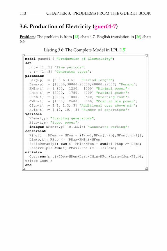
113 CHAPTER 3. PROBLEMS FROM THE GUERET BOOK

3.6. Production of Electricity (guer04-7)

Problem: The problem is from [13] chap 4.7. English translation in [26] chap6.6.

Listing 3.6: The Complete Model in LPL [15]� �model guer04_7 "Production of Electricity";set

p := [1..5] "Time periods";t := [1..3] "Generator types";

parameterLarg{p} := [6 3 6 3 6] "Period length";Dema{p} := [15000,30000,25000,40000,27000] "Demand";PMin{t} := [ 850, 1250, 1500] "Minimal power";PMax{t} := [2000, 1750, 4000] "Maximal power";CDem{t} := [2000, 1000, 500] "Starting cost";CMin{t} := [1000, 2600, 3000] "Cost at min power";CSup{t} := [ 2, 1.3, 3] "Additional cost above min";NDis{t} := [ 12, 10, 5] "Number of generators";

variableNDem{t,p} "Starting generators";PSup{t,p} "Supp. power";integer NFon{t,p} [0..NDis] "Generator working";

constraintR{p,t} : NDem >= NFon - if(p=1,NFon[t,#p],NFon[t,p-1]);Lim{p,t}: PSup <= (PMax-PMin)*NFon;SatisDeman{p}: sum{t} PMin*NFon + sum{t} PSup >= Dema;Reserve{p}: sum{t} PMax*NFon >= 1.15*Dema;

minimizeCost:sum{p,t}(CDem*NDem+Larg*CMin*NFon+Larg*CSup*PSup);

Writep(Cost);end� �

CHAPTER 3. PROBLEMS FROM THE GUERET BOOK 114

3.7. Stadium Construction (guer05-2)

Problem: A municipality wants to construct a small stadium. A constructioncompany is awarded the contract an wants to complete the construction inthe shortest time possible. All tasks are listed and their duration (in weeks) isestimated and the the order of precedence between them is established, thatis, certain tasks must be completetd before others can begin. All these dataare collected in a table (see Table 3.1.

What is the earliest possible date of completing the construction?

The model is from [13] chapter 5.2. and [26] chapter 7.1.

Task Description Duration Predecessors max reduct. add. cost1 Installing the construction site 2 none 02 Terracing 16 1 3 303 Constructing the foundations 9 2 1 264 Access roads and other networks 8 2 2 125 Erecting the basement 10 3 2 176 Main floor 6 4,5 1 157 Dividing up the changing rooms 2 4 1 88 Electrifying the terraces 2 6 09 Constructing the roof 9 4,6 2 42

10 Lighting of the stadium 5 4 1 2111 Installing the terraces 3 6 1 1812 Sealing the roof 2 9 013 Finishing the changing rooms 1 7 014 Constructing the ticket office 7 2 2 2215 Secondary access roads 4 4,14 2 1216 Means of signalling 3 8,11,14 1 617 Lawn and sport accessories 9 12 3 1618 Handing over the building 1 17 0

Table 3.1: Data for the Stadium Construction

Modeling Steps

We introduce a set for the tasks i, j ∈ I. All we need is the duration time of atask pi and the precedence list of task tuples Preci,j. The tuple entry Preci,jis true if and only if task i must be completed before task j. The variables arethe (earliest) starting time ti of a task i. The objective is to minimize the lateststarting time.

The model is as follows:

min maxi∈I

(ti + pi)

subject to tj − ti ≥ pi, ∀(i, j) ∈ Precti ≥ 0, ∀ i ∈ I

115 CHAPTER 3. PROBLEMS FROM THE GUERET BOOK

Listing 3.7: The Model in LPL [15]� �model guer05_2 "Stadium Construction";

set i,j "tasks";Prec{i,j} "precedences";

parameter p{i} "duration";r{i} "max. reduction";c{i} "add. cost per reducted week";T "starting time of last task";

variable t{i} "start time of task i";constraint Precedence{Prec[i,j]}: t[j] - t[i] >= p[i];minimize lasttaskBegin: max{i} (t+p);T:=lasttaskBegin;Writep(T,t);Draw.Scale(14,20);for{i} doDraw.Rect(t,i,p,1,i%12+2); Draw.Text((t+p)&'',t+p,i

+.5,12);Draw.Text(i&'',t+0.1,i+.6,12);Draw.Line(t,i+1,t,#i+2); Draw.Text(t&'',t+.1,#i

+1.8,12);endDraw.Rect(0,#i+2,t[#i],.1,0);--CostModel;EarliestLatest;

end� �Further Comments: A comment on the Read statement: The first read staemetnreads the data from an Excel sheet (the statement is outcommented). The sec-ond Read reads the same data from the same format in a tab separated textfile. Note how similar these statements are. In the text-form we use '%1'to indicate that the first line must be skipped, and '\t\n' indicates that theonly token separators are tabs and line feeds.

Listing 3.8: The Data Modelmodel data;parameter M; string N{i}; PR{i};--Read{i}('guer05-2.xls,[Sheet1$A2:F19]',i,N,p,PR,r,c

);Read{i}('guer05-2.txt,;1,\t\n',i,N,p,PR,r,c);{i,j} (M:=Strfloat(PR[i],',',j), if(M,Prec[M,i]:=1));

end

Question (Answer see 3.8)

1. What is the earliest, what is the latest time that each task can begin?

2. Draw a Gantt diagram to visualiser the solution.

CHAPTER 3. PROBLEMS FROM THE GUERET BOOK 116

3. Suppose that the duration of each task could be reduced by one unit.What is now the solution?

4. Suppose that the task number 4 can only begin at the 32 week. Whatare the implication of the overall plan?

5. Suppose the municipality would like to terminate the construction ear-lier than projected by the construction company and is ready to pay abonus of 30 unit of money for each reduced week. The company hasadditional costs for each task ci per reduced week (last column in Table3.1) and each task can only be reduced a maximal number of weeks,given by ri (second to the last column in Table 3.1. How would theconstruction company proceed?

6. Create and run a project with 100 tasks.

Answer (Question see 3.4)

1. Replace the objective by the following code:

minimize obj: max{i} (t+p) + 0.00001*(sum{i} t);parameter Earliest{i}:=t;minimize obj1: max{i} (t+p) - 0.00001*(sum{i} t);parameter Lastest{i}:=t;

The parameter Earliest gives the eariest possible starting time, andLastest gives the latest possible time. The Submodel EarliestLatestshows the results.

2. See answer 1

3. Repace pi by pi − 1 the run again. The completion time is 55 weeks.

4. Add the constraint constraint C4: t[4]>=32; and run the modelagain.

5. Certainly, the company would try to maximize the additional bonuses.The additional requirements are formulated in the model CostModel.

117 CHAPTER 3. PROBLEMS FROM THE GUERET BOOK

3.8. Flow-shop Scheduling (guer05-3)

Problem: The model is from [13], Chap 5.3. and [26] chapter 7.2.

Listing 3.9: The Complete Model in LPL [15]� �model guer05_3 "Flow-shop Scheduling";

set m,m1 := [1..3] "Machines";j,k,k1 := [1..6] "Job j / Rank k,k1";

parameterp{m,j}:=[3 6 3 5 5 7, 5 4 2 4 4 5, 5 2 4 6 3 6] "

processing time";variableE{m,k|k<#k and m>1} "Idle time on machine m between

job of rang k and k+1";A{m,k|m<#m and k>1} "Waiting time between machine m

and m+1 of job in rang k";binary X{j,k} "1 if job j is in rank k";

constraintC{k}: sum{j} X = 1 "Exactly un job in each rank";B{j}: sum{k} X = 1 "Exactly un rank for each job";D{m,k|m<#m and k<#k}:

E[m,k] + sum{j} p[m,j]*X[j,k+1] + A[m,k+1] =A[m,k] + sum{j} p[m+1,j]*X[j,k] + E[m+1,k]

"Relations between end of job at rang k on mach mand begin of the following job on mach m+1";

minimize W: sum{m,j|m<#m} p*X[j,1]+sum{k|k<#k} E[#m,k]"Total empty time on the last machine";

integer parameterx{j}:=argmax{k|X} k;T{m,k} := sum{m1,j|m1<m} p[m1,j]*X[j,1] +sum{k1,j|k1<k} p[m,j]*X[j,k1] + sum{k1|k1<k} E[m,k1]"begin on mach m of job with rank k";

t{m,j}:=T[m,x];Write('Total wating time: %4d\n', W);Write('Job permutation : %3d\n', {j}x);---draw the solutionDraw.Scale(20,25);for{m,j} do Draw.Rect(j&'',t,m,p,1,j+3); end;set i:=[1..40];for{i} do Draw.Line(i,#m+1,i,#m+1.3); endfor{i} do Draw.Text(i&'',i,#m+1.5,12); end

end� �Question (Answer see 6.8)

1. Visualize the solution with a Gantt diagram.

CHAPTER 3. PROBLEMS FROM THE GUERET BOOK 118

2. How could we force to process job 1 just before job 3 ? Add the condi-tion for that. What is the total duration now?

3. Suppose that we must execute the job 6 as the first job. How could thiscondition be added to the model? What is the consequence on the totalprocessing time?

4. Create and run a problem with 50 jobs.

Answer (Question see 3.7)

1.

119 CHAPTER 3. PROBLEMS FROM THE GUERET BOOK

3.9. Job Shop: non-generic version (guer05-4a)

Problem: The problem is from [13] chap 5.4. English translation in [26] chap7.3.

Listing 3.10: The Complete Model in LPL [15]� �model guer05_4a "Job Shop: non-generic version";set

n := [1..3] "Jobs";m := [1..3] "Machines";

parameterP{m,n}:=[45 20 0 0 10 17 10 34 28] "Process time";M := 1000 "Big-M";

variableT{m,n} "Begin of task";TEnd "Make span";binary Y{1..5} "Disjuctions";

constraintFinJ1 : TEnd >= T[3,1]+P[3,1];FinJ2 : TEnd >= T[3,2]+P[3,2];FinJ3 : TEnd >= T[3,3]+P[3,3];-- Conjonctions : task of the same job on the machinesJ1_M3M1 : T[1,1]+P[1,1] <= T[3,1];J2_M1M3 : T[2,2]+P[2,2] <= T[1,2];J2_M3M2 : T[1,2]+P[1,2] <= T[3,2];J3_M2M3 : T[2,3]+P[2,3] <= T[3,3];-- Disjonctions : precedence on the same machineM1_J1J2_1 : T[1,1]+P[1,1] <= T[1,2]+M-M*Y[1];M1_J1J2_2 : T[1,2]+P[1,2] <= T[1,1]+M*Y[1];M2_J2J3_1 : T[2,2]+P[2,2] <= T[2,3]+M-M*Y[2];M2_J2J3_2 : T[2,3]+P[2,3] <= T[2,2]+M*Y[2];M3_J1J2_1 : T[3,1]+P[3,1] <= T[3,2]+M-M*Y[3];M3_J1J2_2 : T[3,2]+P[3,2] <= T[3,1]+M*Y[3];M3_J1J3_1 : T[3,1]+P[3,1] <= T[3,3]+M-M*Y[4];M3_J1J3_2 : T[3,3]+P[3,3] <= T[3,1]+M*Y[4];M3_J2J3_1 : T[3,2]+P[3,2] <= T[3,3]+M-M*Y[5];M3_J2J3_2 : T[3,3]+P[3,3] <= T[3,2 ]+M*Y[5];

minimize FinOrdo: TEnd;Writep(TEnd,T,Y);end� �

CHAPTER 3. PROBLEMS FROM THE GUERET BOOK 120

3.10. Job Shop: generic version (guer05-4b)

Problem: The problem is from [13] chap 5.4. English translation in [26] chap7.3.

Listing 3.11: The Complete Model in LPL [15]� �model guer05_4b "Job Shop: generic version";set

m,n := [1..9] "Tasks";U{m,n} := [1 7, 5 2, 2 8, 6 9] "m before n";D{m,n} := [1 2, 5 6, 7 8, 7 9, 8 9] "m before n";

parameterP{m} := [45,20,0,0,10,17,10,34,28] "Processing time";M := sum{m} P "Big-M";

variableT{m} "Starting time";TEnd [0..M] "Makespan";binary Y{D[m,n]|m<#m and n>m} "Disjonctions";

constraintToutesTerminees{m}: TEnd >= T+P;Conj{U[m,n]}: T[m]+P[m] <= T[n];Dis1{D[m,n]|m<#m and n>m}: T[m]+P[m] <= T[n]+M*Y;Dis2{D[m,n]|m<#m and n>m}: T[n]+P[n] <= T[m]+M-M*Y;

minimize FinOrdo: TEnd;Writep(FinOrdo,T);end� �

121 CHAPTER 3. PROBLEMS FROM THE GUERET BOOK

3.11. Sequencing jobs on a bottleneck machine(guer05-5)

Problem: The problem is from [13] chap 5.5. English translation in [26] chap7.4.

Listing 3.12: The Complete Model in LPL [15]� �model guer05_5 "Sequencing jobs on a bottleneck machine";set m,n := [1..7] "Job / Rank";parameter

r{m}:=[2 5 4 0 0 8 9] "Earlist time";p{m}:=[5 6 8 4 2 4 2] "Processing time";d{m}:=[10 21 15 10 5 15 22] "Due date";

variablet{n} "Starting time";c{n} "End time";T{n} "Tardiness";binary u{m,n} "Job sequence";

constraintPos{n}: sum{m} u = 1;Job{m}: sum{n} u = 1;Sequence{n|n<#n}: t[n+1] >= t[n] + sum{m} p*u;Debut{n}: t >= sum{m} r*u;Completion{n}: c = t + sum{m} p*u;Retard{n}: T >= c - sum{m} d*u;

minimize Cmax: c[#n];integer parameter M{n}:=argmax{m} u;Draw.Scale(20,20);for{n} do Draw.Rect(M&'',t,1,c-t,1,M+1); endDraw.Text(Cmax&' ',Cmax+1,1.1);

minimize SommeC: sum{n} c;M{n}:=argmax{m} u;for{n} do Draw.Rect(M&'',t,3,c-t,1,M+1); endDraw.Text(Cmax&' ',Cmax+1,3.1);

minimize SommeT: sum{n} T;M{n}:=argmax{m} u;for{n} do Draw.Rect(M&'',t,5,c-t,1,M+1); endDraw.Text(Cmax&' ',Cmax+1,5.1);

Writep(SommeC,Cmax,t);end� �

Question (Answer see 6.12)

1. Implement the three objectifs: (1) minimize the makespan, (2) minimizethe average processing time, (3) minimize the total tardiness.

2. Draw a Gantt diagram.

CHAPTER 3. PROBLEMS FROM THE GUERET BOOK 122

3. Create and run an model with 50 jobs.

123 CHAPTER 3. PROBLEMS FROM THE GUERET BOOK

3.12. Paint production (guer05-6)

Problem: The problem is from [13] chap 5.6. English translation in [26] chap7.5.

Listing 3.13: The Complete Model in LPL [15]� �model guer05_6 "Paint production";set i,j := [1..5] "Periods";parameter

d{i} := [40,35,45,32,50] "Processing time";c{i,j} "Setup time (cleaning time)" :=[ 0,11, 7,13,11 , 5, 0,13,15,1513,15, 0,23,11 , 9,13, 5, 0, 3 , 3, 7, 7, 7, 0

/* 0,7,5,11,6,0 , 6,0,9,9,7,6 , 10,8,0,6,10,10 ,7,12,7,0,6,7 , 7,11,8,11,0,7 */ ];

variable Y{i};binary variable X{i,j|i<>j};constraint

A{i}: sum{j} X = 1;B{j}: sum{i} X = 1;C{i,j|i<>j and j>1}: Y[j] >= Y[i]+1-#i + X*#i;

minimize Cycle: sum{i,j} (d+c)*X;Writep(Cycle);end� �

CHAPTER 3. PROBLEMS FROM THE GUERET BOOK 124

3.13. Assembly line balancing (guer05-7)

Problem: The problem is from [13] chap 5.7. English translation in [26] chap7.6.

Listing 3.14: The Complete Model in LPL [15]� �model guer05_7 "Assembly line balancing";set t := [1..12] "Tasks";

p := [1..4] "Machines";A{t,t} :=

[1 2, 1 3, 2 4, 2 5, 2 6, 3 6, 3 7, 4 9, 5 9,6 8, 7 11, 8 9, 8 10, 9 12, 10 12, 11 10];

parameter D{t}:=[3,6,7,6,4,8,9,11,2,13,4,3] "Proc. time";model gantt,g;variable T{t};constraint prec{A[i,j]}: T[i]+D[i] <= T[j];minimize makespan: sum{t} T;

endgantt;parameter F{t}:= g.T;variable

TT "Cycle time";binary X{t,p} "Assign";

constraintOneMaschPerTask{t}: sum{p} X = 1;Sequence{A[i,j]}: sum{p} p*X[i,p] <= sum{p} p*X[j,p];UpperBound{p}: sum{t} D*X <= TT;

minimize Cycle: TT;Writep(TT);parameter FF{p}:=min{t|X} F;parameter f{t};{p,t|X} (f[t]:=sum{t1 in t|X[t1,p] and t1<t} D[t1]+FF);Draw.Scale(20,20);Draw.DefFont('Verdana',12);Draw.Rect(0,0,50,10,1);{p} Draw.Text('ligne '&p,0,p+.7);{p} Draw.Text(' '&sum{t|X} D,2,p+.7);{p,t|X} Draw.Rect(t&'',f+3,p,D,1,2,0,1);

end� �

125 CHAPTER 3. PROBLEMS FROM THE GUERET BOOK

3.14. Planning the production of bicycles (guer06-2)

Problem: The problem is from [13] chap 6.2. English translation in [26] chap8.1.

Listing 3.15: The Complete Model in LPL [15]� �model guer06_2 "Planning the production of bicycles";set n := [1..12] "Time periods";parameter

D{n} "Demand" := [30000,15000,15000,25000,33000,40000,45000,45000,26000,14000,25000,30000];

CN := 130 "Unit cost, normal time";CS := 160 "Unit cost, over time";CSt := 20 "Storage cost";Capa := 30000 "Production capacilty";SInit := 2000 "Inituial storage";

variableXN{n} [0..Capa] "Quantity to produce, normal time";XS{n} "Quantity to produce, overtime";S{n} "Storage";

constraintPeriode{n}: XN + XS + if(n=1,SInit,S[n-1]) = D + S;

minimize Cost: sum{n} (CN*XN + CS*XS + CSt*S);Writep(Cost);end� �

CHAPTER 3. PROBLEMS FROM THE GUERET BOOK 126

3.15. Production of drinking glasses (guer06-3)

Problem: The problem is from [13] chap 6.3. English translation in [26] chap8.2.

Listing 3.16: The Complete Model in LPL [15]� �model guer06_3 "Production of drinking glasses";set

m := [1..12] "Week periods";n := [1..6] "Products";

parameterCAT := 390 "Workforce capacity";CAM := 850 "Capacity machines";CAZ := 1000 "Storage capacity";d{n,m} "Demand" :=[20, 22, 18, 35, 17, 19, 23, 20, 29, 30, 28, 3217, 19, 23, 20, 11, 10, 12, 34, 21, 23, 30, 1218, 35, 17, 10, 9, 21, 23, 15, 10, 0, 13, 1731, 45, 24, 38, 41, 20, 19, 37, 28, 12, 30, 3723, 20, 23, 15, 10, 22, 18, 30, 28, 7, 15, 1022, 18, 20, 19, 18, 35, 0, 28, 12, 30, 21, 23];

C{n}:=[100 80 110 90 200 140] "Prod cost";CS{n}:=[25 28 25 27 10 20] "Stagage cost";SI{n}:=[50 20 0 15 0 10] "Initial storgae";SF{n}:=[10 10 10 10 10 10] "Min. storage";Tut{n} := [3 3 3 2 4 4] "Workforce time";Tum{n} := [2 1 4 8 11 9] "Machine time";Tzs{n} := [4 5 5 6 4 9] "Storage space";

variableQ{n,m} "Quantity";s{n,m} "Storage";

constraintDem{n,m}: if(m=1,SI,s[n,m-1]) + Q - s = d;CapHom{m}: sum{n} Tut*Q <= CAT "Workforce";CapMac{m}: sum{n} Tum*Q <= CAM "Machine";CapSto{m}: sum{n} Tzs*s <= CAZ "Storage";StockFin{n}: s[n,#m] >= SF "Final storage";

minimize Cost: sum{n,m} C*Q + sum{n,m} CS*s;Writep(Cost);end� �

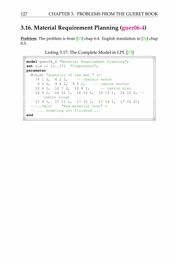
127 CHAPTER 3. PROBLEMS FROM THE GUERET BOOK

3.16. Material Requirement Planning (guer06-4)

Problem: The problem is from [13] chap 6.4. English translation in [26] chap8.3.

Listing 3.17: The Complete Model in LPL [15]� �model guer06_4 "Material Requirement Planning";set n,m := [1..17] "Components";parameter

B{n,m} "Quanlity of raw mat." :=/4 1 2, 4 2 1, -- chassis monte9 3 2, 9 4 2, 9 5 1, -- cabine montee

12 6 1, 12 7 2, 12 8 1, -- camion bleu16 9 1, 16 10 1, 16 12 1, 16 13 1, 16 15 2, --

camion rouge17 9 1, 17 11 1, 17 12 1, 17 14 1, 17 15 2/;

--...CA{n} "Raw material cost" =-- ... modeling not finished ...

end� �

CHAPTER 3. PROBLEMS FROM THE GUERET BOOK 128

3.17. Production of elec. components (guer06-5)

Problem: The problem is from [13] chap 6.5. English translation in [26] chap8.4.

Listing 3.18: The Complete Model in LPL [15]� �model guer06_5 "Production of elec. components";set

m := [1..6] "Time periods";n := [1..4] "Components";

parameterCB := 0.5 "Cost to reduce production";CA := 1.0 "Cost to augment production";d{n,m} "Demand" :=[1500 3000 2000 4000 2000 25001300 800 800 1000 1100 9002200 1500 2900 1800 1200 21001400 1600 1500 1000 1100 1200];

C{n} := [20 25 10 15] "Prod cost";CS{n}:= [.4 .5 .3 .3] "Storage cost";SI{n}:= [10 0 50 0] "Initial stock";SF{n}:= [50 10 30 10] "Stock minimal";

variableQ{n,m} "Prod quantity";s{n,m} "Storage";B{m} "Lower production";A{m} "Raise production";

constraintBal{n,m}: if(m=1,SI,s[n,m-1]) + Q = d+s;Chg{m|m>1}: sum{n} Q + B = sum{n} Q[n,m-1] + A;St{n}: s[n,#m] >= SF;

minimizeCost: sum{n,m}(C*Q+CS*s) + sum{m|m>1}(CB*B+CA*A);

Writep(Cost);end� �

129 CHAPTER 3. PROBLEMS FROM THE GUERET BOOK

3.18. Production of fiberglass (guer06-6)

Problem: The problem is from [13] chap 6.6. English translation in [26] chap8.5.

Listing 3.19: The Complete Model in LPL [15]� �model guer06_6 "Production of fiberglass";set m,n := [1..12] "Periods";parameter

Capa{n} :=[140,100,100,120,110,100,100,90,120,120,100,110];

Arcs{n,m} :=/1 2 5 , 3 4 8 , 5 6 6 , 7 8 6 , 9 10 7 , 11 12 6,2 4 0.2, 4 6 0.3, 6 8 0.2, 8 10 0.25, 10 12 0.3/;

variable x{n,m|Arcs};constraint

Demand{m|m%2=0}: sum{n} x[n,m] = Capa + sum{n} x[m,n];Cap{n|n%2=1}: sum{m} x <= Capa;

minimize Cost: sum{n,m|Arcs} Arcs*x;Writep(Cost);end� �

CHAPTER 3. PROBLEMS FROM THE GUERET BOOK 130

3.19. Assign prod batches to machines (guer06-7)

Problem: The problem is from [13] chap 6.7. English translation in [26] chap8.6.

Listing 3.20: The Complete Model in LPL [15]� �model guer06_7 "Assign prod batches to machines";set

n :=[1..10] "Batches";m :=[1..5] "Machines";

binary variable x{m,n} "Assign";parameter

c{m,n} "Production Cost":= [17 21 22 18 24 15 20 18 19 18

23 16 21 16 17 16 19 25 18 2116 20 16 25 24 16 17 19 19 1819 19 22 22 20 16 19 17 21 1918 19 15 15 21 25 16 16 23 15];

v{m,n} "Processing time":= [ 8 15 14 23 8 16 8 25 9 17

15 7 23 22 11 11 12 10 17 1621 20 6 22 24 10 24 9 21 1420 11 8 14 9 5 6 19 19 78 13 13 13 10 20 25 16 16 17];

Ca{m} "Capacity":= [18 19 25 19 20];

constraintAffectation{n}: sum{m} x = 1;Capacite{m}: sum{n} v*x <= Ca;

minimize Cost: sum{m,n} c*x;Writep(Cost);end� �

131 CHAPTER 3. PROBLEMS FROM THE GUERET BOOK

3.20. Wagon load balancing (guer07-2)

Problem: The problem is from [13] chap 7-2. English translation in [26] chap9.1.

Listing 3.21: The Complete Model in LPL [15]� �model guer07_2 "Wagon load balancing";set

n := [1..16] "Boxes";m := [1..3] "Wagons";

parameter P{n}:=[34,6,8,17,16,5,13,21,25,31,14,13,33,9,25,25] "Weight";

variable CMax "Max charge";binary variable X{n,m} "Assign";constraint

Affect{n}: sum{m} X = 1;RegleCMax{m}: sum{n} P*X <= CMax;--Bound: CMax >= 99; // to speed up the solver

minimize MaxCharge: CMax;Writep(MaxCharge);end� �

CHAPTER 3. PROBLEMS FROM THE GUERET BOOK 132

3.21. Barge loading (guer07-3)

Problem: The problem is from [13] chap 7.3. English translation in [26] chap9.2.

Listing 3.22: The Complete Model in LPL [15]� �model guer07_3 "Barge loading";

set n :=[1..7] "Clients";parameter C:=1500 "Capacity";q{n}:=[ 12 31 20 25 50 40 60] "Av. qty";t{n}:=[ 10 8 6 8 15 10 12] "Lot size";p{n}:=[1000 600 600 700 1200 800 1100] "Price";c{n}:=[ 80 70 85 80 73 70 80] "Trans. cost";g{n}:=p-c*t "Profit";

integer variable x{n} [0..q] "Lots";constraint Capa: sum{n} t*x <= C;maximize Gain: sum{n} g*x;Writep(Gain);

end� �

133 CHAPTER 3. PROBLEMS FROM THE GUERET BOOK

3.22. Tank loading (guer07-4)

Problem: The problem is from [13] chap 7.4. English translation in [26] chap9.3.

Listing 3.23: The Complete Model in LPL [15]� �model guer07_4 "Tank loading";set

q := [1..5] "Liquids";r := [1..9] "Tanks";

parameterCapa{r} := [500,400,400,600,600,900,800,800,800];QIni{r} := [0 ,100, 0, 0, 0, 0,300, 0, 0];LIni{r} := [0 , 1, 0, 0, 0, 0, 5, 0, 0];Arrive{q} := [1200, 700,1000,450,1200];

binary variable X{q,r|QIni=0} "Assign";constraint

PasMixer{r|QIni=0}: sum{q} X <= 1;Suffit{q}: sum{r|QIni=0} Capa*X >=

Arrive - sum{r|LIni=q} (Capa-QIni);minimize FreeCapa: sum{q,r|QIni=0} Capa*X;Writep(FreeCapa);end� �

CHAPTER 3. PROBLEMS FROM THE GUERET BOOK 134

3.23. Backing up files (guer07-5)

Problem: The problem is from [13] chap 7.5. English translation in [26] chap9.4.

Listing 3.24: The Complete Model in LPL [15]� �model guer07_5 "Backing up files";set

n := [1..16] "Files";m := [1..3] "Disks";

parameterA{n} := [26 35 52 77 88 94 137 164 253 364

372 388 406 432 461 851] "File size";B := 1400 "Disk size";

variable NbU "Number of disks used";binary variable X{n,m} "Assign";constraint

NbUtilisees{n}: NbU >= sum{m} m*X;ObjDansUneSeuleBoite{n}: sum{m} X = 1;Capacite{m}: sum{n} A*X <= B;

minimize Nr: NbU;Writep(Nr);end� �

135 CHAPTER 3. PROBLEMS FROM THE GUERET BOOK

3.24. Cutting sheet metal (guer07-6)

Problem: The problem is from [13] chap 7.6. English translation in [26] chap9.5.

Listing 3.25: The Complete Model in LPL [15]� �model guer07_6 "Cutting sheet metal";set

m := [1..4] "Ordered sizes";n := [1..16] "Patterns";

parameterA{m,n} "Pattern table" :=[1 1 1 0 0 0 0 0 0 0 0 0 0 0 0 02 1 0 2 1 0 3 2 1 0 5 4 3 2 1 00 0 0 2 2 2 1 1 1 1 0 0 0 0 0 00 1 3 0 1 3 0 2 3 5 0 1 3 5 6 8];

D{m}:=[8 13 5 15] "Demand";integer variable X{n};constraint Demande{m}: sum{n} A*X >= D;minimize NR: sum{n} X;Writep(NR);end� �

CHAPTER 3. PROBLEMS FROM THE GUERET BOOK 136

3.25. Cutting steel bars for desk legs (guer07-7)

Problem: The problem is from [13] chap 7.7. English translation in [26] chap9.6.

Listing 3.26: The Complete Model in LPL [15]� �model guer07_7 "Cutting steel bars for desk legs";set

p := [1..3] "Leg types";b := [1..2] "Bar types";n := [1..12] "Patterns";

parameterN := 6 "Number per bars";A{n,p} "Pattern table" :=[0 0 2, 0 1 1, 2 0 1, 0 2 0, 2 1 0, 3 0 0 --1.5m0 1 2, 0 2 1, 1 0 2, 3 0 1, 0 3 0, 5 0 0]; --2m

D{p}:=[432 500 400] "Demand";H{p}:=[40 60 70] "Height";L{b}:=[150 200] "Length";

integer variable X{n} "Quantity";constraint Demande{p}: sum{n} A*X >= D;minimize Loss: sum{n} if(n<=N,L[1],L[2])*X -sum{p} D*H;Writep(Loss);end� �

137 CHAPTER 3. PROBLEMS FROM THE GUERET BOOK

3.26. Car rental (guer08-2)

Problem: The problem is from [13] chap 8.2. English translation in [26] chap10.1.

Listing 3.27: The Complete Model in LPL [15]� �model guer08_2 "Car rental";set n,m := [1..10] "Agencies";parameter

C := 3 "Km unit cost";Theo{n} := [10,06,08,11,09,07,15,07,09,12];Reel{n} := [08,13,04,08,12,02,14,11,15,07];X{n} := [00,04,04,06,07,07,01,01,02,00];Y{n} := [00,04,02,02,00,05,05,02,00,03];S{n} := Reel - Theo;D{n,m} := (Abs(X[n]-X[m])^2 + Abs(Y[n]-Y[m])^2)^0.5;

variable Z{n,m|S[n]>0 and S[m]<0};constraint

Surplus{n|S[n]>0}: sum{m|S[m]<0} Z = S[n];Besoins{m|S[m]<0}: sum{n|S[n]>0} Z = -S[m];

minimize Cost: sum{n,m} C*D*Z;Writep(Cost,Z);end� �

CHAPTER 3. PROBLEMS FROM THE GUERET BOOK 138

3.27. Choosing the mode of transport (guer08-3)

Problem: The problem is from [13] chap 8.3. English translation in [26] chap10.2.

Listing 3.28: The Complete Model in LPL [15]� �model guer08_3 "Choosing the mode of transport";

set n,k "Locations";parameterm{n,k} "Lower bound";Ca{n,k} "Upper bound";c{n,k} "Cost";

Read{n,k}('guer08-3.dat', n,k,m,Ca,c);parameterS := 1 "Source";T := #n "Sink";F := 180 "Quantity to transport";

variable p{n,k|Ca} [m,Ca];constraintFlow{n|n<>T and n<>S}: sum{k|Ca[k,n]} p[k,n] =

sum{k|Ca[n,k]} p[n,k];QTY: sum{n|n<>S and Ca[S,n]} p[S,n] = F;

minimize Cost: sum{n,k|Ca} c*p;Writep(Cost);

end� �

139 CHAPTER 3. PROBLEMS FROM THE GUERET BOOK

3.28. Depot location (guer08-4)

Problem: The problem is from [13] chap 8.4. English translation in [26] chap10.3.

Listing 3.29: The Complete Model in LPL [15]� �model guer08_4 "Depot location";set

n := [1..12] "Locations";m := [1..12] "Costumers";

parameterc{n,m} default 1000000 "Cost" :=[100 80 50 50 60 100 120 90 60 70 65 110120 90 60 70 65 110 140 110 80 80 75 130140 110 80 80 75 130 160 125 100 100 80 150160 125 100 100 80 150 190 150 130 . . .190 150 130 . . . 200 180 150 . . .200 180 150 . . . 100 80 50 50 60 100100 80 50 50 60 100 120 90 60 70 65 110120 90 60 70 65 110 140 110 80 80 75 130140 110 80 80 75 130 160 125 100 100 80 150160 125 100 100 80 150 190 150 130 . . .190 150 130 . . . 200 180 150 . . .200 180 150 . . . 100 80 50 50 60 100];

f{n}:=[35 90 100 40 30 90 90 30 40 100 90 35] "Cost";d{m}:=[120 80 75 100 110 100 90 60 30 150 95 120] "

Demand";Ca{n}:=[300 250 100 180 275 300 200 220 270 250 230

180] "Capacity";variable x{n,m} [0,1] "Transport (%)";binary variable y{n} "Assign";constraint

Satisfac{m}: sum{n} x = 1;Capacite{n}: sum{m} d*x <= Ca*y;

minimize Cost: sum{n} 100*f*y + sum{n,m} c*x;Writep(Cost);end� �

CHAPTER 3. PROBLEMS FROM THE GUERET BOOK 140

3.29. Heating oil delivery (guer08-5)

Problem: The problem is from [13] chap 8.5. English translation in [26] chap10.4.

Listing 3.30: The Complete Model in LPL [15]� �model guer08_5 "Heating oil delivery";set n,m := [1..7] "Clients+depot";-- Attention, contrairement au livre, les noeuds sont ici-- indexes dans l'ordre : Donges, Brain, Carquefou,

Guerande,-- Haie Fouassiere, Ponts-de-Ce, Mesanger. Les fichiers

de-- donnees sont reordonnes en consequence.parameter

Qmax := 39000;D{n,m} "distances" :=[0 148 55 32 70 140 73148 0 93 180 99 12 7255 93 0 85 20 83 2832 180 85 0 100 174 9970 99 20 100 0 85 49

140 12 83 174 85 0 7373 72 28 99 49 73 0 ];

Q{n}:=[0 14000 3000 6000 16000 15000 5000] "demand";variable C{n};binary variable X{n,m|n<>m};constraint

enter{n|n>1}: sum{m} X = 1;leave{m|m>1}: sum{n} X = 1;First{n|n>1}: C <= Qmax-(Qmax-Q)*X[1,n];j_Apres_i{n,m|n<>m and n>1 and m>1}: C[m] >= C[n]+Q[m]-

Qmax + Qmax*X[n,m]+(Qmax-Q[m]-Q[n])*X[m,n];Bound{n|n>1}: Q <= C <= Qmax;

minimize kilometres: sum{n,m|n<>m} D*X;Writep(kilometres);end� �

141 CHAPTER 3. PROBLEMS FROM THE GUERET BOOK

3.30. Combining diff modes of transport (guer08-6)

Problem: The problem is from [13] chap 48.6. English translation in [26] chap10.5.

Listing 3.31: The Complete Model in LPL [15]� �model guer08_6 "Combining diff modes of transport";set

n := [1..5] "Locations";m,m1 := [1..3] "Modes (rail, route, air)";

parameterC{m,n}:=[30 40 30 60 . , 20 40 50 50 . , 40 10 60 40

.];T{m,m1}:=[0 2 1, 2 0 1, 2 1 0] "Mode change mode";

binary variableX{m,n|n<#n} "Assign";Y{m,m1,n|n>1 and n<#n} "Change Mode";

constraintUnMode{n|n<#n}: sum{m} X = 1;UnTransf{n|n>1 and n<#n}: sum{m,m1} Y = 1;Cons{n,m,m1|n>1 and n<#n}: X[m,n-1] + X[m1,n] >= 2*Y;

minimize Cost: sum{m,n|n<#n} C*X + sum{n,m,m1|n<#n} T*Y;Writep(Cost);end� �

CHAPTER 3. PROBLEMS FROM THE GUERET BOOK 142

3.31. Fleet planning for vans (guer08-7)

Problem: The problem is from [13] chap 8.7. English translation in [26] chap10.6.

Listing 3.32: The Complete Model in LPL [15]� �model guer08_7 "Fleet planning for vans";set

t := [1..3] "Contracts";m,m1 := [1..6] "Months";

parameterZ := 200 "Initial stock";B{m} := [ 430, 410, 440, 390, 425, 450] "Needs";C{t} := [1700, 2200, 2600] "Cost";

variable Y{t,m} "Number vans";constraint Cover{m}: if(m<=2,Z) + sum{t,m1|m1 >=

Max(1,m-t-1) and m1<=Min(m,#m-t-1)} Y[t,m1] >= B;minimize Cost: sum{t,m} C*Y;Writep(Cost);end� �

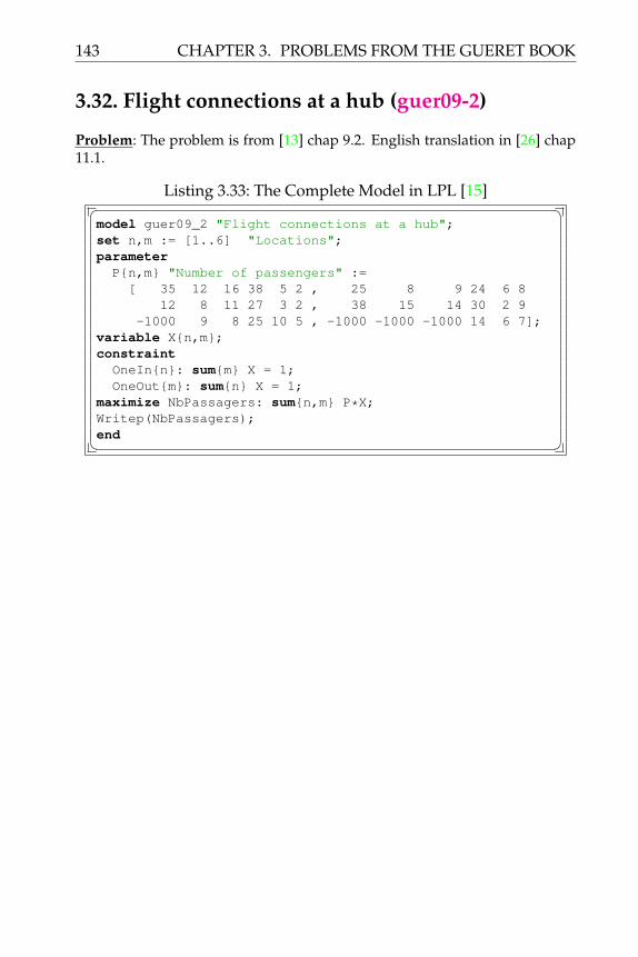
143 CHAPTER 3. PROBLEMS FROM THE GUERET BOOK

3.32. Flight connections at a hub (guer09-2)

Problem: The problem is from [13] chap 9.2. English translation in [26] chap11.1.

Listing 3.33: The Complete Model in LPL [15]� �model guer09_2 "Flight connections at a hub";set n,m := [1..6] "Locations";parameter

P{n,m} "Number of passengers" :=[ 35 12 16 38 5 2 , 25 8 9 24 6 8

12 8 11 27 3 2 , 38 15 14 30 2 9-1000 9 8 25 10 5 , -1000 -1000 -1000 14 6 7];

variable X{n,m};constraint

OneIn{n}: sum{m} X = 1;OneOut{m}: sum{n} X = 1;

maximize NbPassagers: sum{n,m} P*X;Writep(NbPassagers);end� �

CHAPTER 3. PROBLEMS FROM THE GUERET BOOK 144

3.33. Composing flight crews (guer09-3)

Problem: The problem is from [13] chap 9.3. English translation in [26] chap11.2.

Listing 3.34: The Complete Model in LPL [15]� �model guer09_3 "Composing flight crews";set n,m,m1 "Number of pilots";parameter

G{n,m} "Score" :=/1 2 30, 1 4 24, 1 5 25, 2 3 27, 2 4 28, 2 6 27,3 6 26, 3 7 30, 4 5 29, 4 6 21, 5 6 30, 5 8 30,6 7 28, 6 8 36, 7 8 25/;

binary variable X{n,m|G};constraint Sep{n}: sum{m,m1|m=n or m1=n} X[m,m1] <= 1;maximize Score: sum{n,m} G*X;Writep(Score);end� �

145 CHAPTER 3. PROBLEMS FROM THE GUERET BOOK

3.34. Scheduling flight langings (guer09-4)

Problem: The problem is from [13] chap 9.4. English translation in [26] chap11.3.

Listing 3.35: The Complete Model in LPL [15]� �model guer09_4 "Scheduling flight langings";set n,m := [1..10] "Aeroplanes";parameter

M := 1000 "Big-M";inf:=999999;Deb{n}:=[129 195 89 96 110 120 124 126 135 160]

"Begin time window";Fin{n}:=[559 744 510 521 555 576 577 573 591 657]

"End time window";Pre{n}:=[155 258 98 106 123 135 138 140 150 180]

"Prefered time";Ava{n}:= [10 10 30 30 30 30 30 30 30 30]

"Penalty for too early";Ret{n}:= [10 10 30 30 30 30 30 30 30 30]

"Penalty for too late" ;Sep{n,m} "Delay" :=[99999 3 15 15 15 15 15 15 15 153 99999 15 15 15 15 15 15 15 1515 15 99999 8 8 8 8 8 8 815 15 8 99999 8 8 8 8 8 815 15 8 8 99999 8 8 8 8 815 15 8 8 8 99999 8 8 8 815 15 8 8 8 8 99999 8 8 815 15 8 8 8 8 8 99999 8 815 15 8 8 8 8 8 8 99999 815 15 8 8 8 8 8 8 8 99999];

variableT{n} [Deb..Fin] "Langing time";A{n} [0..Pre-Deb] "Too early";R{n} [0..Fin-Pre] "Too late";

binary variable X{n,m|n<m};constraint

cart1{n,m|m<n}: T + Sep <= T[m] + M*X[m,n];Ecart2{n,m|m>n}: T + Sep <= T[m] - M*X[n,m] + M;Avance{n}: A >= Pre - T;Retard{n}: R >= T - Pre;AvOuRe{n}: T = Pre -A + R;

minimize Penalty: sum{n} (Ava*A + Ret*R);Writep(Penalty);end� �

CHAPTER 3. PROBLEMS FROM THE GUERET BOOK 146

3.35. Airline hub location (guer09-5)

Problem: The problem is from [13] chap 9.5. English translation in [26] chap11.4.

Listing 3.36: The Complete Model in LPL [15]� �model guer09_5 "Airline hub location";set n,m,k := [1..6] "Locations";parameter

p := 2 "Number of hubs";Alpha := 80/100 "Cost reduction";D{n,m} "distances" :=[ 0, 870, 702, 4420, 4300, 4380

870, 0, 840, 3660, 3620, 3640702, 840, 0, 4200, 4100, 4140

4420, 3660, 4200, 0, 140, 5714300, 3620, 4100, 140, 0, 5014380, 3640, 4140, 571, 501, 0];

Q{n,m} "transport quantity" :=[ 0, 500, 1000, 300, 400, 15001500, 0, 250, 630, 360, 1140400, 510, 0, 460, 320, 490300, 600, 810, 0, 820, 310400, 100, 420, 730, 0, 970350, 1020, 260, 580, 380, 0];

C{n,m,k,n1 in n}:=D[n,k]+Alpha*D[k,n1]+D[n1,m];binary variable

Z{n,m,k,n1 in n};X{n};

constraintpHubs: sum{n} X = p "Exactly p Hubs";DeuxVilDeuxHubs{n,m} : sum{k,n1 in n} Z[n,m,k,n1] = 1;kHub{n,m,k,n1 in n}: Z[n,m,k,n1] <= X[k];mHub{n,m,k,n1 in n}: Z[n,m,k,n1] <= X[n1];

minimize Cost:sum{n,m,k,n1 in n} C[n,m,k,n1]*Q[n,m]*Z[n,m,k,n1];

Writep(Cost);end� �

147 CHAPTER 3. PROBLEMS FROM THE GUERET BOOK

3.36. Planning a flight tour (guer09-6)

Problem: The problem is from [13] chap 9.6. English translation in [26] chap11.5.

Listing 3.37: The Complete Model in LPL [15]� �model guer09_6 "Planning a flight tour";set n,m := [1..7] "Locations";

--/Bordeaux Lille Lyon Marseille Nantes Paris Toulouse/;

parameterd{n,m} "Distance" :=/1 2 786, 1 3 549, 1 4 657, 1 5 331, 1 6 559,1 7 250, 2 3 668, 2 4 979, 2 5 593, 2 6 224,2 7 905, 3 4 316, 3 5 607, 3 6 472, 3 7 467,4 5 890, 4 6 769, 4 7 400, 5 6 386, 5 7 559,6 7 681/;

binary variable y{n,m};constraint

Entree{m}: sum{n|n<>m} y = 1;Sortie{n}: sum{m|n<>m} y = 1;S1: y[2,6] + y[6,2] <= 1;S2: y[1,7] + y[7,1] <= 1;

minimize Trajet: sum{n,m} if(n<m,d[n,m],d[m,n])*y;Writep(Trajet);end� �

CHAPTER 3. PROBLEMS FROM THE GUERET BOOK 148

3.37. Network reliability (guer10-2)

Problem: The problem is from [13] chap 10.2. English translation in [26] chap12.1.

Listing 3.38: The Complete Model in LPL [15]� �model guer10_2 "Network reliability";

setn,m := [1..11] "nodes";G{n,m} "arcs" :=

[1 2, 1 3, 1 11, 2 3, 2 8, 2 9, 3 4, 3 9, 3 10,3 11, 4 5, 4 6, 4 11, 5 9, 5 11, 6 7, 6 9, 6 10,7 8, 7 10, 8 10, 9 10];;

G{n,m}:=G[n,m] or G[m,n];parameters := 10 "Source";t := 11 "Sink";

variable Phi{n,m|G[n,m] or G[m,n]};constraintA{n|n<>s and n<>t}: sum{m} Phi[m,n] = sum{m} Phi[n,m

];B{n|n<>s and n<>t}: sum{m} Phi[n,m] <= 1;C: sum{n} Phi[n,s] = 0;

maximize Debit: sum{n} Phi[s,n];Writep(Debit);parameter x{n} :=[2 4 2 1 2 4 6 6 4 5 1];

y{n} :=[1 1 2 4 3 4 4 1 3 2 3];Draw.Scale(100,100);{G[n,m]} Draw.Line(x[n],y[n],x[m],y[m],0,if(Phi[n,m

],4,1));{n} Draw.Circle(n&'',x,y,.3,1,0);

end� �

149 CHAPTER 3. PROBLEMS FROM THE GUERET BOOK

3.38. Dimensioning of a mobile phone network(guer10-3)

Problem: The problem is from [13] chap 10.3. English translation in [26] chap12.2.

Listing 3.39: The Complete Model in LPL [15]� �model guer10_3 "Dimensioning of a mobile phone network";set

c := [1..10] "Cells";n := [1..5] "Hubs nodes";

parameterK := 48 "Capacity";C{c,n} "Cost" :=[15 8 7 11 10, 9 11 8 5 14, 12 6 7 15 1517 5 9 18 24, 8 22 21 19 6, 7 25 15 9 1719 25 21 20 22, 20 9 15 18 25, 21 22 14 16 20,25 24 13 4 11];

T{c}:=[22 12 20 12 15 25 15 14 8 22] "traffic";D{c}:=[2 2 2 2 3 1 3 2 2 2 ];

binary variable X{c,n} "Assign";constraint

Divers{c}: sum{n} X = D;CapaciteAnneau: sum{c,n|n<#n} (T/D)*X <= 2*K;

minimize Cost: sum{c,n} C*X;Writep(Cost);end� �

CHAPTER 3. PROBLEMS FROM THE GUERET BOOK 150

3.39. Routing tlephone calls (guer10-4)

Problem: The problem is from [13] chap 10.4. English translation in [26] chap12.3.

Listing 3.40: The Complete Model in LPL [15]� �model guer10_4 "Routing tlephone calls";set

a,b := [1..6] "Nodes";p := [1..5] "Pair numbers";c := [1..17] "Paths";

parameterCapa{a}:=[300,120,300,200, 80, 70] "Capacity";Chem{c,a} "Paths table" :=[2 0 0 0 0 0, 1 3 0 0 0 0, 1 4 6 5 0 0, 1 4 6 0 0 0,1 3 5 0 0 0, 2 5 0 0 0 0, 2 3 4 6 0 0, 1 4 0 0 0 0,2 3 4 0 0 0, 1 3 5 6 0 0, 2 5 6 0 0 0, 2 1 4 0 0 0,3 4 0 0 0 0, 5 6 0 0 0 0, 4 6 0 0 0 0, 1 2 5 0 0 0,3 5 0 0 0 0];

Pi{c}:=[1 1 1 2 2 2 2 3 3 3 3 4 4 4 5 5 5];D{p}:=[100 80 75 100 70] "Demand";

integer variable Phi{c} "Flow";constraint

RespD{p}: sum{c|Pi=p} Phi <= D;RespC{b}: sum{c,a|Chem[c,a]=b} Phi[c] <= Capa[b];

maximize Flow: sum{c} Phi;Writep(Flow);end� �

151 CHAPTER 3. PROBLEMS FROM THE GUERET BOOK

3.40. Construction of a cabled networkt (guer10-5)

Problem: The problem is from [13] chap 10.5. English translation in [26] chap12.4.

Listing 3.41: The Complete Model in LPL [15]� �model guer10_5 "Construction of a cabled networkt";set n,m := [1..6] "nodes";parameter

D{n,m} "Distances" :=[ 0 120 92 265 149 194, 120 0 141 170 93 164, 92 1410 218 103 116, 265 170 218 0 110 126, 149 93 103110 0 72, 194 164 116 126 72 0];

variable Level{n};binary variable X{n,m|n<>m};constraint

NbConnexions: sum{n,m} X = #n-1;Connexe{n,m|m<>n}: Level[m] >= Level[n]+1-#n+#n*X;

minimize Cost: sum{n,m} D*X;Writep(Cost);end� �

CHAPTER 3. PROBLEMS FROM THE GUERET BOOK 152

3.41. Scheduling of telecomm. via satellite(guer10-6)

Problem: The problem is from [13] chap 10.6. English translation in [26] chap12.5.

Listing 3.42: The Complete Model in LPL [15]� �model guer10_6 "Scheduling of telecomm. via satellite";

set n,m := [1..4] "stations";parameterT{n,m}:=[7 12 11 15, 15 8 13 9, 17 12 6 10, 6 13 15

11] "traffic";LB;

binary variable X{n,m|T};variable PMin;constraintUnRecParEme{n}: sum{m} X = 1;UnEmeParRec{m}: sum{n} X = 1;ReglePMin{n}: sum{m} T*X >= PMin;

parameter i:=2;while i>0 domaximize obj: PMin;LB:=LB+PMin;Writep(PMin,T,X);T{n,m}:=if(X=1,T-PMin,T);--if(XX,T-PMin,T);ClearData(X);i:=i-1;

end;Writep(LB);

end� �

153 CHAPTER 3. PROBLEMS FROM THE GUERET BOOK

3.42. Localisation of GSM transmitters (guer10-7)

Problem: The problem is from [13] chap 10.7. English translation in [26] chap12.6.

Listing 3.43: The Complete Model in LPL [15]� �model guer10_7 "Localisation of GSM transmitters";set

n := [1..15] "Villages to deserve";m := [1..7] "Locations of transmitters";Cv{m,n} "Covering" :=[1 1, 1 2, 1 4, 2 2, 2 3, 2 5, 3 4, 3 7, 3 8, 3 10,4 5, 4 6, 4 8, 4 9, 5 8, 5 9, 5 12, 6 7, 6 10, 6 11,6 12, 6 15, 7 12, 7 13, 7 14, 7 15];

parameterB := 10 "Budget maximal";p{n}:=[2,4,13,6,9,4,8,12,10,11,6,14,9,3,6]"Population";c{m}:=[1.8, 1.3, 4.0, 3.5, 3.8, 2.6, 2.1] "Cost";

binary variablex{m} "Transmitter there?";y{n} "Couvered?";

constraintCouvCom{n}: sum{m|Cv} x >= y;Budget: sum{m} c*x <= B;

maximize MaxPop: sum{n} p*y;Writep(MaxPop);end� �

CHAPTER 3. PROBLEMS FROM THE GUERET BOOK 154

3.43. Choice of loans (guer11-2)

Problem: The problem is from [13] chap 11.2. English translation in [26] chap13.1.

Listing 3.44: The Complete Model in LPL [15]� �model guer11_2 "Choice of loans";set

i := [1..3] "Shops";j := [1..3] "Banks";

parametern := 8 "Time horizon";Mmax := 3000000 "Max amount to loan";T{j,i}:=[0.05 0.065 0.061, 0.052 0.062 0.062,

0.055 0.058 0.065] "Interest";P{i}:=[2500000,1000000,1700000] "Price of shop";

variable X{j,i};constraint

A{i}: sum{j} X = P;B{j}: sum{i} X <= Mmax;

minimize Annuities: sum{j,i} X*T/(1-(1+T)^(-n));Writep(Annuities);end� �

155 CHAPTER 3. PROBLEMS FROM THE GUERET BOOK

3.44. Publicity campaign (guer11-3)

Problem: The problem is from [13] chap 11.3. English translation in [26] chap13.2.

Listing 3.45: The Complete Model in LPL [15]� �model guer11_3 "Publicity campaign";set n "Various medias";string parameter nN{n};parameter

ca{n} "Potential";c{n} "Cost";nd{n} "Usage";q{n} "Quality index";B := 250000 "Max budget";C := 100000 "Number of clients to reach";

Read{n}('guer11-3.dat', n,nN,c,ca,q,nd);integer variable m{n} [0..nd];constraint

BudgetMax : sum{n} c*m <= B;CibleMini : sum{n} ca*m >= C;

maximize QualPercep: sum{n} q*m;Writep(QualPercep,m);end� �

CHAPTER 3. PROBLEMS FROM THE GUERET BOOK 156

3.45. Portfolio selection (guer11-4)

Problem: The problem is from [13] chap 11.4. English translation in [26] chap13.3.

Listing 3.46: The Complete Model in LPL [15]� �model guer11_4 "Portfolio selection";set

n := [Dash 'Ilog France' Eurodecision 'Ilog Usa''France Telecom' BNP];

Tech{n} := n<=3;France{n}:= ~(n=1 or n=4);

parameterC := 100000 "Capital";r{n}:=[5.3, 6.2, 5.1, 4.9, 6.5, 3.4] "Interest";

variable v{n} [5000..40000];constraint

Technologiques : sum{Tech} v <= 0.3*C;Francaises : sum{France} v >= 0.5*C;CapitalMaximum : sum{n} v <= C;

maximize RetourTotal: sum{n} r/100*v;Writep(RetourTotal,v);end� �

157 CHAPTER 3. PROBLEMS FROM THE GUERET BOOK

3.46. Finacing an early retirment scheme (guer11-5)

Problem: The problem is from [13] chap 11.5. English translation in [26] chap13.4.

Listing 3.47: The Complete Model in LPL [15]� �model guer11_5 "Finacing an early retirment scheme";set

n := [1..7] "Time horizon";e := [1..3] "Bond types";

parameterTaux := 3.2 "Annual interest rate";F{n}:=[1000 600 640 480 760 1020 950] "Needs";p{e}:=[1.0, 0.8, 0.5] "Priice";t{e}:=[7.0, 7.0, 6.5] "Interestt";T{e} := p*t/100;TotalaPayer:=sum{n} F;

variableCT "Capital";I{n} "Annual investment";integer N{e} [0..5000] "Quantity to buy";

constraintyear1: CT - sum{e} p*N - I[1] = F[1];year{n|n>1 and n<6}:sum{e} T*N+(1+Taux/100)*I[n-1]-I=F;year6: (p[1]+T[1])*N[1] + (p[2] + T[2])*N[2]+ T[3]*N[3] + (1+Taux/100)*I[5] - I[6] = F[6];

year7: (p[3]+T[3])*N[3] + (1+Taux/100)*I[6] = F[7];minimize Capital: CT;Writep(CT,TotalaPayer,N);parameter EE{n}:= if(n<=5,sum{e} p*N,n=6,p[3]*N[3],0);

II{n}:=I;FF{n}:=F;

Draw.Scale(20,-5);{n} Draw.Rect(n,0,1,EE/100,2,0,1);{n} Draw.Rect(n,EE/100,1,II/100,3,0,1);{n} Draw.Rect(n,EE/100+II/100,1,FF/100,4,0,1);

end� �

CHAPTER 3. PROBLEMS FROM THE GUERET BOOK 158

3.47. Family budget (guer11-6)

Problem: The problem is from [13] chap 11.6. English translation in [26] chap13.5.

Listing 3.48: The Complete Model in LPL [15]� �model guer11_6 "Family budget";set

n := [1..12] "Months";i := [VieCourante, Loyer, Voiture, Telephone,

Impots, 'EDF/GDF'] "Expenses";parameter

A := 900 "Public allocations";S := 11500 "Salary";D{i} := [3300, 3800, 2000, 800, 600, 5000] "Expenses";m{i} := [1,1,1,2,4,6] "mensualities";d{n,i} := if(n%m,0,D) "Expenses per month";

variablel{n} [1000..9999999] "Leigure";e{n} "Sauvings";

constraint Bal{n}: sum{i} d + l + e <= S + A + e[n-1];maximize Lei: sum{n} l;Writep(Lei,l,e);end� �

159 CHAPTER 3. PROBLEMS FROM THE GUERET BOOK

3.48. Choice of expansion projects (guer11-7)

Problem: The problem is from [13] chap 11.7. English translation in [26] chap13.6.

Listing 3.49: The Complete Model in LPL [15]� �model guer11_7 "Choice of expansion projects";

seta := [1..5] "Time horizon";n := [1..5] "Projects";

parameterca{a}:=[4.8 6.0 4.8 4.2 3.5] "Capital";c{n,a} "Project cost" :=[1.80 2.40 2.40 1.80 1.501.20 1.80 2.40 0.60 0.501.20 1.00 0 0.48 01.40 1.40 1.20 1.20 1.201.60 2.10 2.50 2.00 1.80];

b{n}:=[10.8 4.8 3.2 4.44 12.25] "Profit";binary variable x{n};constraint Invest{a}: sum{n} c*x <= ca;maximize Profit: sum{n} b*x;Writep(Profit,x);

end� �

CHAPTER 3. PROBLEMS FROM THE GUERET BOOK 160

3.49. Mean variance portfolio (guer11-8)

Problem: The problem is from [13] chap 11.8. English translation in [26] chap13.7.

Listing 3.50: The Complete Model in LPL [15]� �model guer11_8 "Mean variance portfolio";

seti,j := [Hardware Software Show_biz T_bills] "

Investment types";parameterr{i}:=[8 9 12 7] "expected return";V{i,j} "co/variance" :=

[ 4 3 -1 0 , 3 6 1 0-1 1 10 0 , 0 0 0 0];

Target := 8.5 "minimum target yield";variable x{i} "Fraction of investment";binary variable y{i};constraint A: sum{i} x = 1;constraint B: sum{i} r*x >= Target;constraint C: sum{i} y <= 2;constraint D{i}: x <= y;minimize risk: sum{i,j} x[i]*V[i,j]*x[j];Writep(risk,x);

end� �

161 CHAPTER 3. PROBLEMS FROM THE GUERET BOOK

3.50. Assigning personnel to machines (guer12-2)

Problem: The problem is from [13] chap 12.2. English translation in [26] chap14.1.

Listing 3.51: The Complete Model in LPL [15]� �model guer12_2b "Assigning personnel to machines";set n,m := [1..6] "Persons";parameter

P{n,m} "Productivity" :=[13 24 31 19 40 29 , 18 25 30 15 43 2220 20 27 25 34 33 , 23 26 28 18 37 3028 33 34 17 38 20 , 19 36 25 27 45 24];

binary variable X{n,m} "Assign";constraint

UneMachParPers{n}: sum{m} X = 1;UnePersParMach{m}: sum{n} X = 1;

maximize ProdTotale: sum{n,m} P*X;Writep(ProdTotale);--maximize MinProd: min{n} (sum{m} P*X);--Writep(MinProd); //maximize a minimal prodictivity !end� �

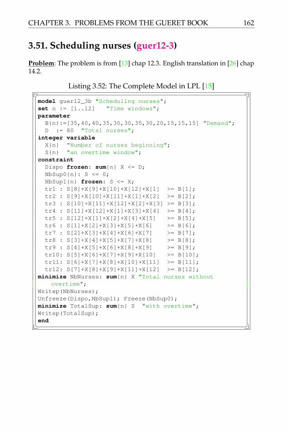
CHAPTER 3. PROBLEMS FROM THE GUERET BOOK 162

3.51. Scheduling nurses (guer12-3)

Problem: The problem is from [13] chap 12.3. English translation in [26] chap14.2.

Listing 3.52: The Complete Model in LPL [15]� �model guer12_3b "Scheduling nurses";set n := [1..12] "Time windows";parameter

B{n}:=[35,40,40,35,30,30,35,30,20,15,15,15] "Demand";D := 80 "Total nurses";

integer variableX{n} "Number of nurses beginning";S{n} "an overtime window";

constraintDispo frozen: sum{n} X <= D;NbSup0{n}: S <= 0;NbSup1{n} frozen: S <= X;tr1 : S[8]+X[9]+X[10]+X[12]+X[1] >= B[1];tr2 : S[9]+X[10]+X[11]+X[1]+X[2] >= B[2];tr3 : S[10]+X[11]+X[12]+X[2]+X[3] >= B[3];tr4 : S[11]+X[12]+X[1]+X[3]+X[4] >= B[4];tr5 : S[12]+X[1]+X[2]+X[4]+X[5] >= B[5];tr6 : S[1]+X[2]+X[3]+X[5]+X[6] >= B[6];tr7 : S[2]+X[3]+X[4]+X[6]+X[7] >= B[7];tr8 : S[3]+X[4]+X[5]+X[7]+X[8] >= B[8];tr9 : S[4]+X[5]+X[6]+X[8]+X[9] >= B[9];tr10: S[5]+X[6]+X[7]+X[9]+X[10] >= B[10];tr11: S[6]+X[7]+X[8]+X[10]+X[11] >= B[11];tr12: S[7]+X[8]+X[9]+X[11]+X[12] >= B[12];

minimize NbNurses: sum{n} X "Total nurses withoutovertime";

Writep(NbNurses);Unfreeze(Dispo,NbSup1); Freeze(NbSup0);minimize TotalSup: sum{n} S "with overtime";Writep(TotalSup);end� �

163 CHAPTER 3. PROBLEMS FROM THE GUERET BOOK

3.52. Establishing a college timetable (guer12-4)

Problem: The problem is from [13] chap 12.4. English translation in [26] chap14.3.

Listing 3.53: The Complete Model in LPL [15]� �model guer12_4 "Establishing a college timetable";set

p := [1..9] "Teachers";c := [1..2] "Classes";td:= [1..20];

parametert := 4 "Time slots per day";d := 5 "Days in a week";NbC{p,c}:=[1 1, 3 3, 2 2, 0 4, 4 0, 3 3, 1 1, 1 0, 0 1]

"Number of courses";string Prf{p}:=['a' 'b' 'c' 'd' 'e' 'f' 'g' 'h' 'i'];variable X{p,c,td} "Assign";constraint

TousPlanif{p,c}: sum{td} X = NbC;Classe{c,td}: sum{p} X <= 1;Prof{p,td}: sum{c} X <= 1;Sport1: X[8,1,15] = 1;Sport2: X[9,2,15] = 1;Devoir{p,c}: X[p,c,1] = 0;Math{td|td<=2}: X[4,2,td] = 0;Biologie{c,td|c<=2 and td>8 and td<13}: X[2,c,td] = 0;AuPlusUn{p,c,td|td<=d}:sum{k in td|k>=(td-1)*t+1 and k<=td*t} X[p,c,k] <= 1;

minimize Trou: sum{p,c,td|td<=d} (X[p,c,(td-1)*t+1]+ X[p,c,(td-1)*t+4]);

parameter Res{c,td} := argmin{p|X} p;string parameter Table{c,td} := Prf[Res];Writep(Trou);end� �

CHAPTER 3. PROBLEMS FROM THE GUERET BOOK 164

3.53. Exam scheduling (guer12-5)

Problem: The problem is from [13] chap 12.5. English translation in [26] chap14.4.

Listing 3.54: The Complete Model in LPL [15]� �model guer12_5a "Exam scheduling";set

e,f := ['Analyse de donnees','Analyse numerique','C++','Genie logiciel','Gestion de production','Java','Modeles et Algorithmique','Programmation logique','Programmation mathematique', 'Statistiques','Systemes a evenements discretes'];t := ['1:8-10h','1:10-12','1:14-16','1:16-18','2:8-10h

','2:10-12','2:14-16','2:16-18'];

--e,f := [1..11];--t := [1..8];

parameterIncomp{e,f} "Incompatibles" :=[0 1 0 0 1 0 1 0 0 1 1 , 1 0 0 0 1 0 1 0 0 1 10 0 0 1 1 1 1 0 1 1 1 , 0 0 1 0 1 1 1 0 0 1 11 1 1 1 0 1 1 1 1 1 1 , 0 0 1 1 1 0 1 0 1 1 11 1 1 1 1 1 0 1 1 1 1 , 0 0 0 0 1 0 1 0 0 1 10 0 1 0 1 1 1 0 0 1 1 , 1 1 1 1 1 1 1 1 1 0 11 1 1 1 1 1 1 1 1 1 0];

binary variable X{e,t} "Assign";constraint

AllScheduled{e}: sum{t} X = 1 "Each exam takes place";Incomp1{e,f,t|Incomp}: X[e,t] + X[f,t] <= 1;--T{t}: Sum{e} X <= 1;

--maximize any: X[1,1]+X[2,2];minimize length: sum{e,t} t^2 * X;---binary variable Y{t} <- or{e} X;---minimize tranche_horaire: sum{t} Y;--maximize tranche: sum{e} X[e,3];Write(' %10s\n', {t}t);Write{e}('%31s %10s\n', e, {t} if (X,'X',' '));model data1 "larger data set (for testing)";

e := [1..100];t := [1..20];Incomp{e,f|e<>f}:=if(e<f and Rnd(0,1)<.4,1);Incomp{e,f|e>f}:=Incomp[f,e];

endend� �

165 CHAPTER 3. PROBLEMS FROM THE GUERET BOOK

3.54. Personnel assignment (guer12-6)

Problem: The model is from [13], Chapter 12.6. and [26].

Modeling Steps

Listing 3.55: The Complete Model in LPL [15]� �model guer12_6 "Personnel assignment";set

n "Products";L,L1 "Production lines";

parameterg{n} "Gain";d{n,L} "Processing time";m{L} "Time capacity";T{L,L1} "Transfert possible";tm{L} "Max hours to transfert";

variableq{n} "Quantity";h{L} "Work hours";t{L,L1|T} "Hours transfered";

constraintChargeLigne{L}: sum{n} d*q <= m;Travail{L}: sum{n} d*q <= h;Equilibrage{L1}: h - sum{L|T[L,L1]} t[L,L1] + sum{L|T[

L1,L]} t[L1,L] = m;MaxTranfert{L}: sum{L1|T=1} t <= tm;

expression Profit: sum{n} g*q;maximize obj1: Profit subject_to ChargeLigne;Writep(Profit,q);maximize obj2: Profit subject_to Travail,Equilibrage,

MaxTranfert;Writep(Profit,q);model data; --- in the book

n := [1..4];L := [1..5];g{n} := [7, 8, 9, 7];d{n,L} :=[1.3, 0.9, 2.0, 0.3, 0.91.8, 1.7, 1.4, 0.6, 1.11.3, 1.2, 1.3, 1.0, 1.40.9, 1.1, 1.0, 0.9, 1.0];

m{L} := [4500, 5000, 4500, 1500, 2500];T{L,L1} := /1 2 1, 1 3 1, 1 4 1, 2 3 1, 2 5 1,3 1 1, 3 2 1, 3 4 1, 4 5 1, 5 1 1, 5 2 1, 5 3 1/;

tm{L} := [400 800 200 500 300];

CHAPTER 3. PROBLEMS FROM THE GUERET BOOK 166

endmodel data1; --- a random data set

n := [1..20];L := [1..5];g{n} := Trunc(Rnd(6,10));d{n,L} := Trunc(Rnd(10,20))/10;m{L} := Trunc(Rnd(1500,6000));T{L,L1|L<>L1} := if(Rnd(0,1)<.3,1,0);tm{L} := Trunc(Rnd(200,900));

endend� �

167 CHAPTER 3. PROBLEMS FROM THE GUERET BOOK

3.55. Personnel at a construction site (guer12-7)

Problem: The problem is from [13] chap 12.7. English translation in [26] chap14.6.

Listing 3.56: The Complete Model in LPL [15]� �model guer12_7 "Personnel at a construction site";set n := [1..6] "Time horizon";parameter

CouArr := 100 "Arrival cost";CouDep := 160 "Departure cost";CouSur := 200 "Overtime cost";CouSou := 200 "Undertime cost";EffDeb := 3 "Initial needs";EffFin := 3 "Final needs";Besoin{n} := [4,6,7,4,6,2] "Needs";

integer variableXEff{n};XArr{n} [0..3];XDep{n};XSur{n};XSou{n};

constraintSatisf{n}: XEff - XSur + XSou = Besoin;PremierMois: XEff[1] = EffDeb + XArr[1];DernierMois: EffFin = XEff[#n] - XDep[#n];Autres{n|n>1}: XEff = XEff[n-1] + XArr - XDep[n-1];Dep{n}: XDep <= (1/3)*XEff;Sou{n}: XSou <= (1/4)*XEff;

minimize Cost: sum{n} (CouArr*XArr + CouDep*XDep + CouSur

*XSur + CouSou*XSou);Writep(Cost);end� �

CHAPTER 3. PROBLEMS FROM THE GUERET BOOK 168

3.56. Water conveyance mamangement (guer13-2)

Problem: The problem is from [13] chap 13.2. English translation in [26] chap15.1.

Listing 3.57: The Complete Model in LPL [15]� �model guer13_2 "Water conveyance mamangement";set n,m := [1..12] "nodes";parameter

s := #n-1 "Source";t := #n "Sink";Capa{n,m} :=/1 3 20, 1 5 15, 1 6 12, 2 5 6, 2 6 22, 3 4 15,3 5 10, 4 8 7, 4 9 10, 5 8 10, 5 9 15, 5 10 15,6 7 22, 7 9 10, 7 10 10, 8 12 18, 9 12 15, 10 12 20,11 1 35, 11 2 25/;

variable Phi{n,m|Capa} [0..Capa];constraint FL{n|n<>s and n<>t}:

sum{m} Phi[n,m] = sum{m} Phi[m,n];maximize Flow: sum{n} Phi[n,t];Writep(Flow);

end� �

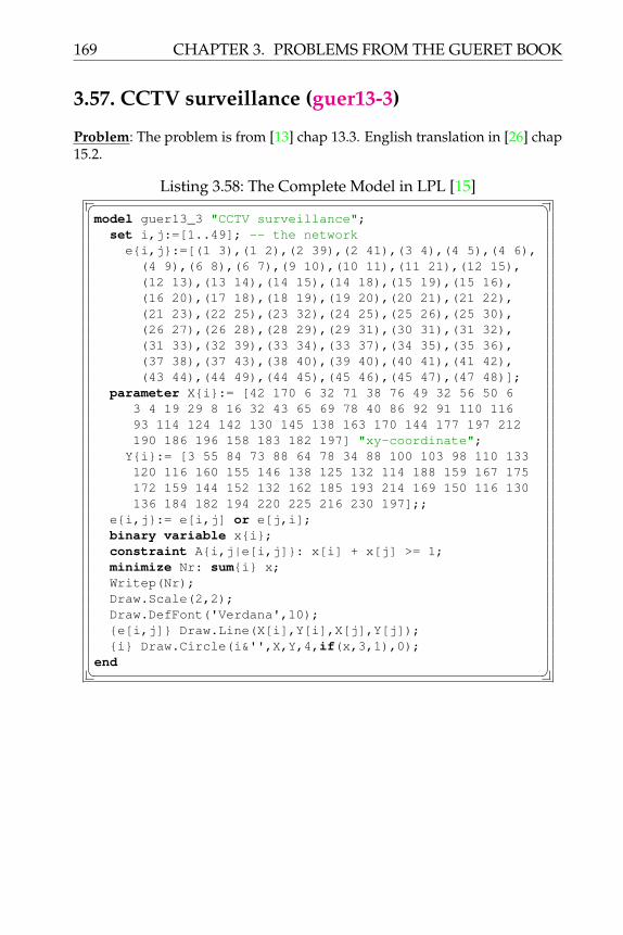
169 CHAPTER 3. PROBLEMS FROM THE GUERET BOOK

3.57. CCTV surveillance (guer13-3)

Problem: The problem is from [13] chap 13.3. English translation in [26] chap15.2.

Listing 3.58: The Complete Model in LPL [15]� �model guer13_3 "CCTV surveillance";

set i,j:=[1..49]; -- the networke{i,j}:=[(1 3),(1 2),(2 39),(2 41),(3 4),(4 5),(4 6),(4 9),(6 8),(6 7),(9 10),(10 11),(11 21),(12 15),(12 13),(13 14),(14 15),(14 18),(15 19),(15 16),(16 20),(17 18),(18 19),(19 20),(20 21),(21 22),(21 23),(22 25),(23 32),(24 25),(25 26),(25 30),(26 27),(26 28),(28 29),(29 31),(30 31),(31 32),(31 33),(32 39),(33 34),(33 37),(34 35),(35 36),(37 38),(37 43),(38 40),(39 40),(40 41),(41 42),(43 44),(44 49),(44 45),(45 46),(45 47),(47 48)];

parameter X{i}:= [42 170 6 32 71 38 76 49 32 56 50 63 4 19 29 8 16 32 43 65 69 78 40 86 92 91 110 11693 114 124 142 130 145 138 163 170 144 177 197 212190 186 196 158 183 182 197] "xy-coordinate";

Y{i}:= [3 55 84 73 88 64 78 34 88 100 103 98 110 133120 116 160 155 146 138 125 132 114 188 159 167 175172 159 144 152 132 162 185 193 214 169 150 116 130136 184 182 194 220 225 216 230 197];;

e{i,j}:= e[i,j] or e[j,i];binary variable x{i};constraint A{i,j|e[i,j]}: x[i] + x[j] >= 1;minimize Nr: sum{i} x;Writep(Nr);Draw.Scale(2,2);Draw.DefFont('Verdana',10);{e[i,j]} Draw.Line(X[i],Y[i],X[j],Y[j]);{i} Draw.Circle(i&'',X,Y,4,if(x,3,1),0);

end� �

CHAPTER 3. PROBLEMS FROM THE GUERET BOOK 170

3.58. Rigging elections (guer13-4)

Problem: A complete problem description and how to model it mathemati-cally is explained in [13], Chapter 13.4.

Modeling Steps

Listing 3.59: The Complete Model in LPL [15]� �model guer13_4 "Rigging elections";set

q := [1..14] "Quarters";c := [1..46] "Districts";

parameterR := 6;M{c}:= [0,0,1,1,0,0,0,1,0,1,1,1,1,1,0,0,0,1,1,0,

0,0,0,0,0,0,1,1,1,0,0,0,0,0,1,1,1,1,1,1,0,1,1,0,0,1];

A{c,q} := /*$I 'guer13-4.dat' */ ;binary variable X{c};constraint

Partition{q}: sum{c} A*X = 1;NombreRequis: sum{c} X = R;

minimize NombreSieges: sum{c} M*X;Writep(NombreSieges,X);end� �

171 CHAPTER 3. PROBLEMS FROM THE GUERET BOOK

3.59. Gritting roads (guer13-5)

Problem: Leaving from his home post office, a postman needs to visit thehouseholds on each block in his route, delivering and collecting letters, andthen returning to the post office. He would like to cover this route by travel-ling the minimum possible distance. The post office is located at the intersec-tion point 1, (see Figure 3.1).

Figure 3.1: The village streets ([26] p.324)

The problem is from [13] Chap 13.5, and from [26] Chap 15.4.

Modeling Steps

The problem can be formulated as a Min Cost Flow Problem, see mcf-a1 forthe general Min Cost Flow problem. That is, we “simulate” the traversing ofan arc as a “flow”. Flow=1 means that the arc is traversed once, flow=2 meansthat the arc is traversed two times, etc. The variables are the number of flowson each arcs (xi,j i, j ∈ V V is the set of route intersections). The flow oneach arc must be 1 (at least on traversal li,j ≤ xi,j. We do not want to limitthe number of flows on each arc, hence we can set ui,j = ∞, however on canshow that 2 is enough (ui,j = 2). So there is: li,j ≤ xi,j ≤ ui,j.

Furthermore, the number of entering a node (intersection) must be exactly thenumber of leaving the node. Hence we have:

1 http://lpl.virtual-optima.com/lpl/Solver.jsp?name=/mcf-a

CHAPTER 3. PROBLEMS FROM THE GUERET BOOK 172

∑j

xi,j −∑j

xj,i = 0 ∀ i ∈ V

Hence, we have a Min Cost Flow Problem with the following specifications:(1) All lower bounds are 1 (li,j = 1, to make sure that all streets are traversedat least once. All upper bound must be at least 2 (ui,j ≥ 2). And for complet-ing the formulation (of a Min Cost Flow), bi = 0 for all nodes.

Listing 3.60: The Complete Model in LPL [15]� �model guer13_5 "Gritting roads";

set i,j := [1..12] "Intersection points";parameterc{i,j} "Steet distances" :=/1 2 150, 1 5 165, 2 3 130, 2 5 230, 2 6 160,3 2 140, 3 4 100, 4 3 100, 4 8 190, 5 1 165,5 6 144, 6 2 170, 6 5 144, 6 7 128, 6 9 218,6 10 174,7 3 200, 7 6 122, 7 8 109, 7 11 185,8 4 180, 8 11 141,8 12 190,9 5 194, 9 10 148,10 6 174,10 7 233,11 7 185,11 10 135,12 11 110/;

l{i,j}:=1;u{i,j}:=999;

variable x{i,j|c} [l..u] "Nr of passing the street";constraint A{i}: sum{j} x[i,j] = sum{j} x[j,i];minimize Distance: sum{i,j} c*x;Writep(Distance);-- draw the graph --parameter X{i}:=2*(i-1)%4; Y{i}:=2*Ceil(i/4);Draw.Scale(60,60);Draw.DefFont('Verdana',12);--{c[i,j]} Draw.CArrow('('&l&','&x&',&#8734;)\n'&'c='&c

,-- X[i],Y[i],X[j],Y[j],.4,.2,0);{c[i,j]} Draw.CArrow(c&'',X[i],Y[i],X[j],Y[j],.4,.2,0);{c[i,j]|x=2} Draw.CArrow(X[i],Y[i],X[j],Y[j],.2,.2,0);{i} Draw.Circle(i&'',X,Y,.2,1,0);

end� �Solution: The optimal traveled distance is 5990. There are 7 arcs that mustbe traversed two times: the first time serving the street and the second timewithout serving. The solution is shown in 3.1

173 CHAPTER 3. PROBLEMS FROM THE GUERET BOOK

Figure 3.2: The minimal traversing

CHAPTER 3. PROBLEMS FROM THE GUERET BOOK 174

3.60. Location of income tax offices (guer13-6)

Problem: The problem is from [13] chap 13.6. English translation in [26] chap15.5.

Listing 3.61: The Complete Model in LPL [15]� �model guer13_6 "Location of income tax offices";set n,m := [1..12] "Locations";parameter

p := 3 "Number of offices";D{n,m} "Distance)" :=-- 1 2 3 4 5 6 7 8 9 10 11 12-------------------------------------------------[ 0, 15, 37, 55, 24, 60, 18, 33, 48, 40, 58, 67

15, 0, 22, 40, 38, 52, 33, 48, 42, 55, 61, 6137, 22, 0, 18, 16, 30, 41, 28, 20, 58, 39, 3955, 40, 18, 0, 34, 12, 59, 46, 24, 62, 43, 3424, 38, 16, 34, 0, 36, 25, 12, 24, 47, 37, 4360, 52, 30, 12, 36, 0, 57, 42, 12, 50, 31, 2218, 33, 41, 59, 25, 57, 0, 15, 45, 22, 40, 6133, 48, 28, 46, 12, 42, 15, 0, 30, 37, 25, 4648, 42, 20, 24, 24, 12, 45, 30, 0, 38, 19, 1940, 55, 58, 62, 47, 50, 22, 37, 38, 0, 19, 4058, 61, 39, 43, 37, 31, 40, 25, 19, 19, 0, 2167, 61, 39, 34, 43, 22, 61, 46, 19, 40, 21, 0];

H{n}:=[15,10,12,18,5,24,11,16,13,22,19,20] "Popul.";binary variable Y{m};variable X{n,m};constraint

Affect{n}: sum{m} X = 1;NbBureaux: sum{m} Y = p;Ajust{n,m}: X <= Y;

minimize DistPondTot: sum{n,m} H*D*X;Writep(DistPondTot);end� �

175 CHAPTER 3. PROBLEMS FROM THE GUERET BOOK

3.61. Efficiency of hospitals (guer13-7)

Problem: The problem is from [13] chap 13.7. English translation in [26] chap15.6.

Listing 3.62: The Complete Model in LPL [15]� �model guer13_7b "Efficiency of hospitals";set

n := [1..4] "Hospitals";K := [1..4] "Services indicators";L := [1..3] "Resource indicators";

parameterh := 2 "Performance measuring on 2 hospitals";s{K,n} "service indication" :=[30.12, 18.54, 20.88, 10.4213.54, 14.45, 8.52, 17.7413, 7, 8, 2679, 55, 47, 50 ];

r{L,n} "resource indication" :=[90, 87, 51, 6638.89, 109.48, 40.43, 48.4134, 33, 20, 33 ];

variableE "Efficiency index";c{n} "Coefficients for method DEA";sf{K} "Fictive service indicateurs";rf{L} "Fictive resource indicateurs";

constraintDEACoefs: sum{n} c = 1;ServFict{K} : sf = sum{n} s*c;RessFict{L} : rf = sum{n} r*c;ServSup{K} : sf >= s[K,h];RessInf{L}: rf <= r[L,h]*E;

minimize Efficiency: E;Writep(Efficiency);end� �

CHAPTER 3. PROBLEMS FROM THE GUERET BOOK 176

3.62. MasterMind (guer14-2)

Problem: The problem is from [13] chap 14.2.

Listing 3.63: The Complete Model in LPL [15]� �model guer14_2 "MasterMind";set

c := [Blanc,Bleu,Jaune,Noir,Rouge,Vert];p := [1..4] "Nombre de positions";

binary variable X{p,c} "=1 si la couleur j est a laposition i";

constraint-- Une couleur doit etre affectee a chaque positionUneCoulParPos{p} : sum{c} X = 1;--Essai 1: 1 couleur bien placee, 1 couleur mal placeeE1_bp: X[1,'Rouge']+X[2,'Jaune']+X[3,'Blanc']+X[4,'Vert

'] = 1;E1_mp: sum{p|p<>1} X[p,'Rouge']+sum{p|p<>2} X[p,'Jaune

'] +sum{p|p<>3} X[p,'Blanc']+sum{p|p<>4} X[p,'Vert'] = 1;

--Essai 2: 1 couleur bien placeeE2_bp: X[1,'Bleu']+X[2,'Vert']+X[3,'Blanc']+X[4,'Bleu']

= 1;E2_mp: sum{p|p<>1 and p<>4} X[p,'Bleu']+sum{p|p<>2} X[p

,'Vert'] +sum{p|p<>3} X[p,'Blanc'] = 0;

--Essai 3: 1 couleur bien placee, 1 couleur mal placeeE3_bp: X[1,'Jaune']+X[2,'Noir']+X[3,'Blanc']+X[4,'Noir

'] = 1;E3_mp: sum{p|p<>1} X[p,'Jaune']+sum{p|p<>2 and p<>4} X[

p,'Noir'] +sum{p|p<>3} X[p,'Blanc'] = 1;

--Essai 4: 4 couleurs mal placeesE4_bp: X[1,'Bleu']+X[2,'Jaune']+X[3,'Rouge']+X[4,'Noir

'] = 0;E4_mp: sum{p|p<>1} X[p,'Bleu'] + sum{p|p<>2} X[p,'

Jaune'] +sum{p|p<>3} X[p,'Rouge']+sum{p|p<>4} X[p,'Noir']=4;

solve;Writep(X);end� �

177 CHAPTER 3. PROBLEMS FROM THE GUERET BOOK

3.63. Probleme de logique sur le marathon de Paris(guer14-3)

Problem: The model is from [13], Chapter 14.3. and [26].

Listing 3.64: The Complete Model in LPL [15]� �model guer14_3 "Probleme de logique sur le marathon de

Paris";set

n := [1..6] "places";c := [Dominique,Ignace,Naren,Olivier,Philippe,Pascal] "

Coureurs";variable X{c,n};constraint

UnePlaceParCoureur{c}: sum{n} X = 1;UnCoureurParPlace{n}: sum{c} X = 1;-- Information a)a: X['Olivier',6] = 0;-- Information b)b: sum{n|n>4} (X['Dominique',n] + X['Ignace',n] + X['

Pascal',n]) = 0;-- Information c)c1: X['Dominique',1] + X['Dominique',2] = 1;-- Information d)d: sum{n|n<=4} X['Philippe',n] = 1;-- Information e)e: X['Ignace',2] + X['Ignace',3] = 0;-- Information f)f1: sum{n|n<=3} X['Naren',n] = 0;f2: sum{n|n>=4} X['Pascal',n] = 0;-- Information g)g: X['Ignace',4] + X['Dominique',4] = 0;

maximize any: X[1];Writep(X);end� �

CHAPTER 3. PROBLEMS FROM THE GUERET BOOK 178

3.64. Chercheurs dans un Congres (guer14-4)

Problem: Probleme de logique consistant a retrouver la nationalite et la dated’expose de 5 chercheurs participant a un congres. The model is from [13],Chapter 14.4.

Listing 3.65: The Complete Model in LPL [15]� �model guer14_4 "Chercheurs dans un Congres";set

Chercheurs,c:=[Arabinda,Eric,Hitoshi,Michael,Zhicheng];n := [Americain,Chinois,Francais,Indien,Japonais];Dates,d := ['7','8','9','10','11'];

variable X{c,n,d};constraint

Chercheur {c}: sum{n,d} X = 1;Nationalite{n}: sum{c,d} X = 1;Dat{d}: sum{c,n} X = 1;-- Information a)a: sum{d} X['Michael','Japonais',d] = 0;-- Information b)b: sum{d|d<=3} X['Eric','Francais',d] = 1;-- Information c)c1: sum{n} X['Arabinda',n,'9'] = 1;-- Information d)d_1: sum{d} (X['Hitoshi','Chinois',d] + X['Michael','

Chinois',d]) = 0;d_2: sum{c} X[c,'Chinois','8'] = 1;d_3: sum{n,d|d>2} X['Michael',n,d] = 1;-- Information e)e_1: sum{n} (X['Hitoshi',n,'7'] + X['Hitoshi',n,'11'])

= 0;e_2: sum{c,d|d>=4} X[c,'Indien',d] = 0;e_3: sum{c,d|d<=2} X[c,'Americain',c] = 0;e_4: sum{d} (X['Hitoshi','Americain',d] + X['Hitoshi','

Indien',d]) = 0;maximize any: X[1];Writep(X);end� �

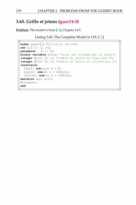
179 CHAPTER 3. PROBLEMS FROM THE GUERET BOOK

3.65. Grille et jetons (guer14-5)

Problem: The model is from [13], Chapter 14.5.

Listing 3.66: The Complete Model in LPL [15]� �model guer14_5 "Grille et jetons";set n,m := [1..4];parameter P := 10;binary variable x{n,m} "(n,m) est occupee par un jeton";integer NL{n} [0..2] "nombre de jetons en ligne par 2";integer NC{n} [0..2] "nombre de jetons en colonne par 2";constraint

Total: sum{n,m} x = P;Lig{n}: sum{m} x = 2*NL[n];Col1{m}: sum{n} x = 2*NC[m];

maximize any: x[1];Writep(x);end� �

CHAPTER 3. PROBLEMS FROM THE GUERET BOOK 180

3.66. Partage de tonneaux entre des neveux(guer14-6)

Problem: The model is from [13], Chapter 14.6.

Listing 3.67: The Complete Model in LPL [15]� �model guer14_6 "Partage de tonneaux entre des neveux";set

n := [1..5] "Nombre de neveux";T := [Plein '3/4' Moite '1/4' Vide]"Nombre de type de tonneaux differents (en contenu)";

parameterr{T} := [1.00, 0.75, 0.50, 0.25, 0.00]"remplissage des tonneaux, plein, 3/4, 1/2, 1/4 et

vide";c{T} := [10000, 1000, 100, 10, 1]"Coefficients pour la contrainte tous differents";

variable p{n} "Valeur du produit scalaire c(_).x(i,_)";integer variable x{n,T} [1..5]

"Nombre de tonneaux de type T donnes au neveu n";constraint

Neveux{n} : sum{T} x = 9;Tonneaux{T} : sum{n} x = 9;Equitable{n}: sum{T} r*x = 4.5;TousDiff{n} : sum{T} c*x = p;Ordre{n|n>1}: p - p[n-1] >= 1;

minimize any: x[1];Writep(p,x);end� �

181 CHAPTER 3. PROBLEMS FROM THE GUERET BOOK

3.67. Le probleme des n reines (guer14-7)

Problem: The model is from [13], Chapter 14.7..

Listing 3.68: The Complete Model in LPL [15]� �model guer14_7 "Le probleme des n reines";set n,m := [1..100];binary variable c{n,m} "une case de l'echiquier vaut 1

si une reine est sur cette case, 0 sinon.";constraint

Ligne{n} : sum{m} c <= 1;Colonne{m} : sum{n} c <= 1;DiagDL{m} : sum{n|n>=m} c[n-m+1,n] <= 1;DiagDC{n|n>1}: sum{m|m>=n} c[m,m-n+1] <= 1;DiagGL{m} : sum{n|n<=m} c[n,m-n+1] <= 1;DiagGC{n|n>1}: sum{m|m>=n} c[m,#n-m+n] <= 1;

maximize NbReines: sum{n,m} c "le nombre de reines";Writep(NbReines,c);end� �

CHAPTER 4

VARIOUS TEXTBOOKS

4.1. Forestry Production Planning (forestry)

Problem: Wood-D Industries has just signed contracts for the clear felling ofthree large forest tracts of second-growth radiata pines. The harvested treeswill supply the firm’s sawmill and chipboard plant. Some of the logging out-put is also available for export. All trees harvested are cut on location intosections 20 feet long, referred to as first cuts, second cuts, etc. On the basis ofa detailed survey of each forest, the firm’s chief forester estimated the averagecomposition of each forest’s total output as shown below:

Log Cuts Forest A Forest B Forest C---------------------------------------------------------First and Second 42% 46% 45%Third and Fourth 40% 41% 45%Fifth and over 18% 13% 10%

---------------------------------------------------------

The average daily output is 128 HC for forest A, 192 HC for forest B, and 200HC for forest C (1 HC = 100 cubic feet = 2.832 cubic meter). The log cutsare sorted onto logging trucks for transportation to either the sawmill or thechipboard plant, the two facilities being at different locations. Transportationcosts per HC are given in the following table:

Transportation Sawmill Chipboard-------------------------------------------Forest A $4 $7Forest B $3 $5Forest C $6 $3

-------------------------------------------

Handling costs per HC is given in the table below:

Handling Sawmill Chipboard-------------------------------------------First and Second $2.5 $1.2Third and Fourth $3.5 $1.5

183

CHAPTER 4. VARIOUS TEXTBOOKS 184

Fifth and over $5.0 $2.0-------------------------------------------

At the sawmill, logs are sawn into three grades of finished products: cleargrade, dressing grade, and construction grade. A substantial fraction of theincoming volume of wood ends up as scrap and sawdust. The table belowshows the average log conversion factors at the sawmill, as well as the averageprocessing rates. Excluding breakdowns, the productive capacity at the millaverages 360 minutes per day.

Sawn Timber Scraps Sawdust ProcessingLogCuts MBF/HC HC/HC HC/HC Time per HC

----------------------------------------------------1-2 0.72 0.26 0.14 1.83-4 0.66 0.30 0.15 2.65- 0.54 0.39 0.16 3.9

----------------------------------------------------

From sample logs processed at the sawmill, average yields for each grade ofsawn timber were determined. They are summarized in the following table.

Clear Dressing Construction----------------------------------------

LogCuts A B C A B C A B C/Forest

--------------------------------------------------1-2 35% 28% 20% 48% 42% 30% 17% 30% 50%3-4 10% 3% 25% 18% 9% 30% 72% 88% 45%5- 0 0 5% 5% 0 30% 95% 100% 65%

--------------------------------------------------

The ex-mill wholesale price per MBF is $150 for clear grades, $110 for dressinggrades and $80 for construction grades. Scraps at the sawmill are transferredby truck to the chipboard plant for chipping. The transportation cost is $4per HC. Sawdust is used as fuel in the mill’s drying kiln and saves $12 inother fuel costs per HC. At the chipboard plants, logs and scraps are chipped.The chips are then mixed with additive glues, filled into 4’ by 8’ forms andthen compressed into boards of various thicknesses. The whole process ishighly automated. Each HC of wood yields 0.76M3/4 of chipboard (1M3/4= 1000 square feet of 3.4 thickness = 1.77 cubic meters). The plant can pro-duce upto 112M3/4 of chipboard per day. Chipboard prices ex-factory are$105 per M3/4. In light of predicted demand and desired stock levels, cer-tain minimum daily output rates of finished product are set up by Wood-Dmanagement for given planning period. These are 31 MBF of clear grades, 35MBF of dressing grade, 48 MBF of construction grade, and 96 M3/4 of chip-board. Export prices valid during the same planning period are $95 per HCfor first and second cuts, and $88 per HC for third and fourth cuts. Fifth or

185 CHAPTER 4. VARIOUS TEXTBOOKS

higher cuts are not exported. The problem is to determine the optimal dailyoperating policy during the planning period in question.

Project Formulate the production planning problem as a linear program usingMPL. Summarize the optimal daily operating policy for the planning prob-lem.

Reference: Prof. Ariela Sofer, Operations Research Dept., George Mason Uni-versity Based on a problem from the book ’Introduction to Operations Re-search Techniques’ by Hans G. Daellenbach, John A. George, and Donald C.McNickle, 1983

CHAPTER 4. VARIOUS TEXTBOOKS 186

4.2. Wyndor Glass Company (hill03-1-1)

Problem:

A complete problem description and how to model it mathematically is clearlyexplained in [12], Example 3.1-1, Page 25. A mathematical model formulation

is:

Listing 4.1: The Complete Model in LPL [15]� �model hill03_1_1 "Wyndor Glass Company";

setp := [Door, Window] "Products";f := [1..3] "Plants";

parameterTimeAvail{f} := [4, 12, 18];ProdTime{f,p} := [1, 0, 0, 2, 3, 2];Profit{p} := [3.00, 5.00];

variable Produce{p};constraintTimeCapacity{f}: sum{p} ProdTime*Produce <= TimeAvail

;maximize TotalProfit: sum{p} Profit*Produce;Writep(TotalProfit,Produce);

end� �

187 CHAPTER 4. VARIOUS TEXTBOOKS

4.3. Mary’s Radiation Therapy (hill03-4-1)

Problem:

A complete problem description and how to model it mathematically is clearlyexplained in [12] , Example 3.4-1, Page 44 A mathematical model formulation

is:

Listing 4.2: The Complete Model in LPL [15]� �model hill03_4_1 "Mary's Radiation Therapy";

setb := [Beam1, Beam2] "Beam";a := [CriticalTissues, TumorRegion, CenterTumor] "

BodyArea";parameterHealthyAnatomy{b} := [0.4, 0.5];DosageAbsorbed{b,a} := [0.3, 0.5, 0.6, 0.1, 0.5,

0.4];Restriction{a} := [2.7, 6.0, 6.0];K{a} := [1 2 3];

variable D{b} "Dosage";constraintDosage1{a|K=1}: sum{b} DosageAbsorbed*D <=

Restriction;Dosage2{a|K=2}: sum{b} DosageAbsorbed*D =

Restriction;Dosage3{a|K=3}: sum{b} DosageAbsorbed*D >=

Restriction;minimize TotalHealthyDosage: sum{b} HealthyAnatomy*D;Writep(TotalHealthyDosage,D);

end� �

CHAPTER 4. VARIOUS TEXTBOOKS 188

4.4. Kibbutzim Crop Allocation (hill03-4-2)

Problem:

A complete problem description and how to model it mathematically is clearlyexplained in [12] , Example 3.4-2, Page 46 A mathematical model formulation

is:

Listing 4.3: The Complete Model in LPL [15]� �model hill03_4_2 "Kibbutzim Crop Allocation";

setk := [1..3] "Kibbutz";c := [SugarBeets, Cotton, Sorghum] "Crops";

parameterUsableLand{k} := [400, 600, 300]; -- {Acres}WaterAlloc{k} := [600, 800, 375]; -- {

AcreFeet}WaterUsed{c} := [3, 2, 1]; -- {

AcreFeet/Acre}NetReturn{c} := [1000, 750, 250]; -- {$/Acre}MaxQuota{c} := [600, 500, 325]; -- {Acres}

variable AllocAcre,A{c,k};constraintMaxLandUse{k}: sum{c} A <= UsableLand;MaxWaterAlloc{k}: sum{c} WaterUsed*A <= WaterAlloc;TotalAcreage{c}: sum{k} A <= MaxQuota;EqProp{k}: sum{c} A/UsableLand = sum{c} A[c,k%#k+1]/

UsableLand[k%#k+1];maximize TotalProfit: sum{c,k} NetReturn*A;Writep(TotalProfit,A);

end� �

189 CHAPTER 4. VARIOUS TEXTBOOKS

4.5. Nori/Leets Air Pollution (hill03-4-3)

Problem:

A complete problem description and how to model it mathematically is clearlyexplained in [12] , Example 3.4-3, Page 50 A mathematical model formulation

is:

Listing 4.4: The Complete Model in LPL [15]� �model hill03_4_3 "Nori/Leets Air Pollution";

setpollutant,p := [Particulates, SulfurOxides,

Hydrocarbons];furnace,f := [Blast, OpenHearth];abatementa,a := [TallerSmokestacks, Filters,

BetterFuels];parameterRequiredReduction{p} := [60, 150, 125];ReducedEmissionRate,rer{p,a,f} :=

[12, 9, 25, 20, 17, 13,35, 42, 18, 31, 56, 49,37, 53, 28, 24, 29, 20];

AnnualCost{a,f} := [8, 10, 7, 6, 11, 9];variable U{a,f} [0..1] "Used Method";constraintEmissionReduction{p}: sum{f,a} rer*U >=

RequiredReduction;minimize TotalCost: sum{a,f} AnnualCost*U;Writep(TotalCost,U);

end� �

CHAPTER 4. VARIOUS TEXTBOOKS 190

4.6. Save-It Company (hill03-4-4)

Problem:

A complete problem description and how to model it mathematically is clearlyexplained in [12] , Example 3.4-4, Page 53 A mathematical model formulation

is:

Listing 4.5: The Complete Model in LPL [15]� �model hill03_4_4 "Save-It Company";

setg := [A, B, C] "Grade";m := [1..4] "Material";GradeMat{g,m} := [A 1, A 2, A 3, A 4, B 1, B 2, B 4,

C 1];parameterMinMixSpecs{g,m} :=

/A 1 0, A 2 0.40, A 3 0 , A 4 0.2,B 1 0, B 2 0.1, B 4 0.1, C 1 0/;

MaxMixSpecs{g,m} :=/A 1 0.3, A 2 0, A 3 0.5, A 4 0.2,B 1 0.5, B 2 0, B 4 0.1, C 1 0.7/;

AmalgamationCost{g} := [3.00, 2.50, 2.00];SellingPrice{g} := [8.50, 7.00, 5.50];MaterialAvail{m} := [3000, 2000, 4000, 1000];TreatmentCost{m} := [3.00, 6.00, 4.00, 5.00];MinimumTreated := 0.5;TreatmentCashAvail := 30000;

variable M{g,m} "MixMaterial";constraintMinMixtureSpecs{g,m|MinMixSpecs>0}: M >= MinMixSpecs

*(sum{m} M);MaxMixtureSpecs{g,m|MaxMixSpecs>0}: M <= MaxMixSpecs

*(sum{m} M);MaterialLimit{m}: sum{g} M <= MaterialAvail;ReqAmountTreated{m}: sum{g} M >= MinimumTreated*

MaterialAvail;TreatCostRestrict: sum{g,m} TreatmentCost*M =

TreatmentCashAvail;maximize TotalProfit: sum{g,m} SellingPrice*M - sum{g,m

} AmalgamationCost*M;Writep(TotalProfit,M);

end� �

191 CHAPTER 4. VARIOUS TEXTBOOKS

4.7. Save-It Company (hill03-4-4b)

Problem: lternative formulation for the same model, adds summary vari-ables.

A complete problem description and how to model it mathematically is clearlyexplained in [12] , Example 3.4-4b, Page 53 A mathematical model formula-

tion is:

Listing 4.6: The Complete Model in LPL [15]� �model hill03_4_4b "Save-It Company";

set grade,g := [A, B, C];material,m := [1..4];GradeMat{g,m}:=[A 1, A 2, A 3, A 4, B 1, B 2,B 4,C

1];parameterMinMixSpecs{g,m} :=/A 1 0, A 2 0.40, A 3 0, A 4 0.20,B 1 0, B 2 0.10, B 4 0.10, C 1 0/;

MaxMixSpecs{g,m} :=/A 1 0.3, A 2 0, A 3 0.50, A 4 0.20,B 1 0.50, B 2 0, B 4 0.10, C 1 0.70/;

AmalgamationCost{g} := [3.00, 2.50, 2.00];SellingPrice{g} := [8.50, 7.00, 5.50];MaterialAvail{m} := [3000, 2000, 4000, 1000];TreatmentCost{m} := [3.00, 6.00, 4.00, 5.00];MinimumTreated := 0.5;TreatmentCashAvail := 30000;

variableG{g} "ProduceGrade";U{m} "MaterialUsed";M{g,m} "MixMaterial";

constraintGradeProd{g}: G = sum{m} M ;MatUse{m} : U = sum{g} M ;MinMixtureSpecs{g,m|MinMixSpecs>0}:M>=MinMixSpecs*G;MaxMixtureSpecs{g,m|MaxMixSpecs>0}:M<=MaxMixSpecs*G;MaterialLimit{m}: U <= MaterialAvail;ReqAmountTreated{m}: U >= MinimumTreated*

MaterialAvail;TreatCostRestrict: sum{m} TreatmentCost*U =

TreatmentCashAvail;maximize TotalProfit: sum{g} SellingPrice*G - sum{g}

AmalgamationCost*G;Writep(TotalProfit,G,U,M);

end� �

CHAPTER 4. VARIOUS TEXTBOOKS 192

4.8. Union Airways Personnel (hill03-4-5)

Problem:

A complete problem description and how to model it mathematically is clearlyexplained in [12] , Example 3.4-5, Page 57 A mathematical model formulation

is:

Listing 4.7: The Complete Model in LPL [15]� �model hill03_4_5 "Union Airways Personnel";

sets := [1..5] "Shifts";p := [AM_6_8, AM_8_10, AM_10_12,

PM_12_2, PM_2_4, PM_4_6, PM_6_8,PM_8_10, PM_10_12, AM_12_6] "Periods";

ShiftSchedule{s,p} :=[1 AM_6_8, 1 AM_8_10, 1 AM_10_12, 1 PM_12_2,2 AM_8_10, 2 AM_10_12, 2 PM_12_2, 2 PM_2_4,3 PM_12_2, 3 PM_2_4, 3 PM_4_6, 3 PM_6_8,4 PM_4_6, 4 PM_6_8, 4 PM_8_10, 4 PM_10_12,5 PM_10_12, 5 AM_12_6];

parameterMinAgentsNeeded{p} := [48, 79, 65, 87, 64, 73, 82,

43, 52, 15];DailyCostPerAgent{s} := [170, 160, 175, 180, 195];

variable A{s} "Assign agents to s";constraintMeetRequirements{p}: sum{s|ShiftSchedule} A >=

MinAgentsNeeded;minimize TotalCost: sum{s} DailyCostPerAgent*A;Writep(TotalCost,A);

end� �

193 CHAPTER 4. VARIOUS TEXTBOOKS

4.9. Distribution Unlimited (hill03-4-6)

Problem:

A complete problem description and how to model it mathematically is clearlyexplained in [12] , Example 3.4-6, Page 59 A mathematical model formulation

is:

Listing 4.8: The Complete Model in LPL [15]� �model hill03_4_6 "Distribution Unlimited";

set i,j := [F1, F2, DC, W1, W2] "Locations";parameterShipCost{i,j} :=/F1 F2 200, F1 DC 400, F1 W1 900, F2 DC 300,DC W2 100, W1 W2 300, W2 W1 200/;

Supply{i} := /F1 50, F2 40/;Demand{i} := /W1 30, W2 60/;MaxFlow{i,j} := /F1 F2 10, DC W2 80/;

variable Ship{i,j|ShipCost};constraintNetFlow{i}: sum{j} Ship[j,i] + Supply

= sum{j} Ship[i,j] + Demand;MaxShipment{i,j|MaxFlow}: Ship <= MaxFlow;

minimize TotalCost: sum{i,j} ShipCost*Ship;Writep(TotalCost,Ship);

end� �

CHAPTER 4. VARIOUS TEXTBOOKS 194

4.10. Wyndor Glass (hill07-1-1)

Problem:

A complete problem description and how to model it mathematically is clearlyexplained in [12] , Example 7.1-1, Page 311 A mathematical model formula-

tion is:

Listing 4.9: The Complete Model in LPL [15]� �model hill07_1_1 "Wyndor Glass";

setp := [Door, Window] "Products";f := [1..3] "Plants";

parameterTimeAvail{f} := [4, 12, 18];ProdTime{f,p} := [1, 0, 0, 2, 3, 2];Profit{p} := [3.00, 5.00];

variable T{f} "Assign agents to f";constraint ProduceDual{p}: sum{f} ProdTime*T >= Profit;minimize TProfit: sum{f} TimeAvail*T;Writep(TProfit,T);

end� �

195 CHAPTER 4. VARIOUS TEXTBOOKS

4.11. Upper Bound (hill07-3-1)

Problem:

A complete problem description and how to model it mathematically is clearlyexplained in [12] „ Example 7.3-1, Page 319 A mathematical model formula-

tion is:

Listing 4.10: The Complete Model in LPL [15]� �model hill07_3_1 "Upper Bound";

setactivity1,a := [Activity1,Activity2,Activity3];constraint1,c := [constraint1,constraint2];

parameterResourceAvail{c} := [12,4];ResourceUse{c,a} := [4,1,0, -2,0,1];UnitProfit{a} := [2,1,2];Upper{a} := [4,15,6];

variable Produce{a} [0..Upper];constraintTimeCapacity{c}: sum{a} ResourceUse*Produce <=

ResourceAvail;maximize TotalProfit: sum{a} UnitProfit*Produce;Writep(TotalProfit,Produce);

end� �

CHAPTER 4. VARIOUS TEXTBOOKS 196

4.12. Goal Programming (hill07-5-1)

Problem:

A complete problem description and how to model it mathematically is clearlyexplained in [12] , Example 7.5-1, Page 333 A mathematical model formula-

tion is:

Listing 4.11: The Complete Model in LPL [15]� �model hill07_5_1 "Goal Programming";

setp := [1..3] "Products";f := [Profit, Employment, Investment] "Factors";d := ['Over', 'Under'] "Deviations";

parameterGoal{f} := [125, 40, 55];PenaltyWeight{d,f} := [0, 2, 3, 5, 4, 0];UnitContrib{f, p} := [12, 9,15, 5, 3, 4, 5, 7,

8];variableProdRate{p};Amount{f,d|PenaltyWeight>0};

constraintCalc{f}: sum{p} ProdRate*UnitContrib

= Goal + Amount[f,'Over'] - Amount[f,'Under'];minimize WeightedSum: sum{d,f} PenaltyWeight*Amount;Writep(WeightedSum,Amount);

end� �

197 CHAPTER 4. VARIOUS TEXTBOOKS

4.13. P-T Company (hill08-1-1)

Problem:

A complete problem description and how to model it mathematically is clearlyexplained in [12] , Example 8.1-1, Page 351 A mathematical model formula-

tion is:

Listing 4.12: The Complete Model in LPL [15]� �model hill08_1_1 "P-T Company";

setcannery,c := [C1, C2, C3];warehouse,w := [W1, W2, W3, W4];

parameterShipCost{c,w} := [464, 513, 654, 867,

352, 416, 690, 791,995, 682, 388, 685];

Supply{c} := [75,125,100];Demand{w} := [80, 65, 70, 85];

variable Ship{c,w};constraintOutput{c}: sum{w} Ship = Supply;Allocation{w}: sum{c} Ship = Demand;

minimize TotalCost: sum{c,w} ShipCost*Ship;Writep(TotalCost,Ship);

end� �

CHAPTER 4. VARIOUS TEXTBOOKS 198

4.14. Northern Airplane (hill08-1-2)

Problem:

A complete problem description and how to model it mathematically is clearlyexplained in [12] „ Example 8.1-2, Page 359 A mathematical model formula-

tion is:

Listing 4.13: The Complete Model in LPL [15]� �model hill08_1_2 "Northern Airplane";

setproduce,p := [1..4];install,i := [1..5];

parameterM := 999;DistCost{p,i} := [1.080, 1.095, 1.110, 1.125, 0,

999, 1.110, 1.125, 1.140, 0,999, 999, 1.100, 1.115, 0,999, 999,999, 1.130, 0];

Supply{p} := [25, 35, 30, 10];Demand{i} := [10, 15, 25, 20, 30];

variable Engines{p,i};constraintProduction{p}: sum{i} Engines = Supply;Installations{i}: sum{p} Engines = Demand;

minimize TotalCost: sum{p,i} DistCost*Engines;Writep(TotalCost,Engines);

end� �

199 CHAPTER 4. VARIOUS TEXTBOOKS

4.15. Metro Water (hill08-1-3)

Problem:

A complete problem description and how to model it mathematically is clearlyexplained in [12] , Example 8.1-3, Page 362 A mathematical model formula-

tion is:

Listing 4.14: The Complete Model in LPL [15]� �model hill08_1_3 "Metro Water";

setr := [Colombo, Sacron, Calorie, Dummy] "Rivers";c := [Berdoo_min, Berdoo_extra, LosDevils, SanGo,

Hollyglass] "Cities";parameterM := 999;DistCost{r, c} := [16, 16, 13, 22, 17,

14, 14, 13, 19, 15,19, 19, 20, 23, 999,

999, 0,999, 0, 0];Supply{r} := [50, 60, 50, 50];Demand{c} := [30, 20, 70, 30, 60];

variable Distribute{r,c};constraintSource{r}: sum{c} Distribute = Supply;Destination{c}: sum{r} Distribute = Demand;

minimize TotalCost: sum{r,c} 10000000*DistCost*Distribute;

Writep(TotalCost,Distribute);end� �

CHAPTER 4. VARIOUS TEXTBOOKS 200

4.16. Job Shop Company (hill08-3-1)

Problem:

A complete problem description and how to model it mathematically is clearlyexplained in [12] , Example 8.3-1, Page 381 A mathematical model formula-

tion is:

Listing 4.15: The Complete Model in LPL [15]� �model hill08_3_1 "Job Shop Company";

setm := [m1, m2, m3, Dummy] "Machines";p := [1..4] "Locations";

parameterM := 999;DistCost{m, p} := [13, 16, 12, 11,

15,999, 13, 20,5, 7, 10, 6,0, 0, 0, 0];

Supply{m} := [1, 1, 1, 1];Demand{p} := [1, 1, 1, 1];

variable Assign{m,p};constraintSource{m}: sum{p} Assign = Supply;Destination{p}: sum{m} Assign = Demand;

minimize TotalCost: sum{m,p} DistCost*Assign;Writep(TotalCost,Assign);

end� �

201 CHAPTER 4. VARIOUS TEXTBOOKS

4.17. Better Products Company (hill08-3-2a)

Problem:

A complete problem description and how to model it mathematically is clearlyexplained in [12] , Example 8.3-2a, Page 386 A mathematical model formula-

tion is:

Listing 4.16: The Complete Model in LPL [15]� �model hill08_3_2a "Better Products Company";

setf := [1..3] "Plants";p := [1..5] "Products";

parameterM := 999;DistCost{f, p} := [41, 27, 28, 24, 0,

40, 29,999, 23, 0,37, 30, 27, 21, 0];

Supply{f} := [75, 75, 45];Demand{p} := [20, 30, 30, 40, 75];

variable Assign{f,p};constraintSource{f}: sum{p} Assign = Supply;Destination{p}: sum{f} Assign = Demand;

minimize TotalCost: sum{f, p} DistCost*Assign;Writep(TotalCost,Assign);

end� �

CHAPTER 4. VARIOUS TEXTBOOKS 202

4.18. Better Products Company (hill08-3-2b)

Problem:

A complete problem description and how to model it mathematically is clearlyexplained in [12] , Example 8.3-2b, Page 386 A mathematical model formula-

tion is:

Listing 4.17: The Complete Model in LPL [15]� �model hill08_3_2b "Better Products Company";

setf := [p1a, p1b, p2a, p2b, p3] "Plants";p := [1..5] "Products";

parameterM := 99999;Cost{f, p} := [820, 810, 840, 960, 0,

820, 810, 840, 960, 0,800, 870,99999, 920, 0,800, 870,99999, 920, 0,740, 900, 810, 840,99999];

binary variable Assign{f, p};constraintAssignee{f}: sum{p} Assign = 1;Task{p}: sum{f} Assign = 1;

minimize TotalCost: sum{f, p} Cost*Assign;Writep(TotalCost,Assign);

end� �

203 CHAPTER 4. VARIOUS TEXTBOOKS

4.19. Shortest Path (hill09-3-1)

Problem:

A complete problem description and how to model it mathematically is clearlyexplained in [12] , Example 9.3-1, Page 411 A mathematical model formula-

tion is:

Listing 4.18: The Complete Model in LPL [15]� �model hill09_3_1 "Shortest Path";

set i,j := [O, A, B, C, D, E, T];parameterDistance{i,j} :=

/O A 2, O B 5, O C 4, A B 2, A D 7, B C 1,B D 4, B E 3, C E 4, D E 1, D T 5, E T 7/;

variable Path{i,j|Distance>0};constraintFlowBalance{i}: if(i='O',1) + sum{j} Path[j,i]

= if(i='T',1) + sum{j} Path[i,j];minimize TotalDistance: sum{i,j} Distance*Path;Writep(TotalDistance,Path);

end� �

CHAPTER 4. VARIOUS TEXTBOOKS 204

4.20. Maximum Flow (hill09-5-1)

Problem:

A complete problem description and how to model it mathematically is clearlyexplained in [12] , Example 9.5-1, Page 420 A mathematical model formula-

tion is:

Listing 4.19: The Complete Model in LPL [15]� �model hill09_5_1 "Maximum Flow";

setnode,i,j := [O, A, B, C, D, E, T];SourceNode{i} := [O];DestNode{i} := [T];

parameterCapacity{i,j} :=

/O A 5, O B 7, O C 4, A B 1, A D 3, B C 2,B D 4, B E 5, C E 4, D T 9, E D 1, E T 6/;

variableFlow{i,j|Capacity>0} [0..Capacity];Entrance{node|node='O'};Destination{node|node='E'};

constraintFlowBal{node}: Entrance + sum{i} Flow[i,node]

= Destination + sum{j} Flow[node,j];maximize TotalFlow: Entrance['O'];Writep(TotalFlow,Flow);

end� �

205 CHAPTER 4. VARIOUS TEXTBOOKS

4.21. Minimum Cost (hill09-6-1)

Problem:

A complete problem description and how to model it mathematically is clearlyexplained in [12] , Example 9.6-1, Page 429 A mathematical model formula-

tion is:

Listing 4.20: The Complete Model in LPL [15]� �model hill09_6_1 "Minimum Cost";

setnode,i,j := [A, B, C, D, E];

parameterUnitCost{i,j} :=/A B 2, A C 4, A D 9, B C 3, C E 1, D E 3, E D

2/;Capacity{i,j} := /A B 10, C E 80/;SupplyDemand{node} := [50, 40, 0, -30, -60];

variable Ship{i,j|UnitCost>0};constraintFlowBalance{node}: sum{i} Ship[i,node] + SupplyDemand

= sum{j} Ship[node,j];MaxCapacity{i,j|Capacity>0}: Ship <= Capacity;

minimize TotalCost: sum{i,j} UnitCost*Ship;Writep(TotalCost,Ship);

end� �

CHAPTER 4. VARIOUS TEXTBOOKS 206

4.22. Critical Path (hill10-1-1)

Problem: RT/PERT Method

A complete problem description and how to model it mathematically is clearlyexplained in [12] , Example 10.1-1, Page 469 A mathematical model formula-

tion is:

Listing 4.21: The Complete Model in LPL [15]� �model hill10_1_1 "Critical Path";

setn,m := [A,B,C,D,E,F,G,H,I,J,K,L,M,N,Finish];Path{n,m} :=

[ A B, B C, C D, C E, C I, D G, E F, E H, F J,G H, H M, I J, J K, J L, K N, L N, M Finish, N

Finish];parameter Duration{n} :=

[2,4,10,6,4,5,7,9,7,8,4,5,2,6,0];variable S{n} "StartTime";constraint SeqRelation{Path[n,m]}: S[n] + Duration[n]

<= S[m];minimize FinishTime: S['Finish'];Writep(FinishTime,S);

end� �

207 CHAPTER 4. VARIOUS TEXTBOOKS

4.23. Crashing (hill10-5-1)

Problem: ritical Path

A complete problem description and how to model it mathematically is clearlyexplained in [12] , Example 10.5-1, Hillier and Lieberman, Page 494 A mathe-

matical model formulation is:

Listing 4.22: The Complete Model in LPL [15]� �model hill10_5_1 "Crashing";

setn,m := [A,B,C,D,E,F,G,H,I,J,K,L,M,N];Path{n,m} :=

[A B, B C, C D, C E, C I, D G, E F, E H, F J,G H, H M, I J, J K, J L, K N, L N];

parameterNormalTime{n} := [2,4,10,6,4,5,7,9,7,8,4,5,2,6];CrashTime{n} := [1,2,7,4,3,3,4,6,5,6,3,3,1,3];NormalCost{n} := [180, 320, 620, 260, 410, 180, 900,

200, 210, 430, 160, 250, 100, 330];CrashCost{n} := [280, 420, 860, 340, 570, 260, 1020,

380, 270, 490, 200, 350, 200, 510];MaxReduce{n} := NormalTime - CrashTime;CostWeekSaved{n} := CrashCost/MaxReduce - NormalCost/

MaxReduce;variableS{n} "StartTime";F [0..40] "Finished";R{n} [0..MaxReduce] "ReducedTime";

constraintSeqRelation{Path[n,m]}: S[n] + NormalTime[n] - R[n]

<= S[m];M: S['M'] + NormalTime['M'] - R['M'] <= F;N: S['N'] + NormalTime['N'] - R['N'] <= F;

minimize TotalCost: sum{n} NormalCost + sum{n}CostWeekSaved*R;

Writep(TotalCost,S,F,R);end� �

CHAPTER 4. VARIOUS TEXTBOOKS 208

4.24. Calif. Manufacturing (hill12-1-1)

Problem: acility Location

A complete problem description and how to model it mathematically is clearlyexplained in [12] , Example 12.1-1, Page 577 A mathematical model formula-

tion is:

Listing 4.23: The Complete Model in LPL [15]� �model hill12_1_1 "Calif. Manufacturing";

setlocation,lo:= [WLA, FLA, WSF, FSF];

parameterNPV{lo} := [6, 9, 4, 5]; -- In millionsCapital{lo} := [5, 6, 2, 3]; -- In millions

binary variable x{lo};constraintBudget: sum{lo} Capital*x <= 10;Warehouse: sum{lo|lo<#lo} x <= 1;Cnt{lo|lo>1}: -x + x[lo+2] <= 0;

maximize TotalNPV: sum{lo} NPV*x;Writep(TotalNPV,x);

end� �

209 CHAPTER 4. VARIOUS TEXTBOOKS

4.25. Production Rates (hill12-4-1)

Problem:

A complete problem description and how to model it mathematically is clearlyexplained in [12] , Example 12.4-1, , Page 592 A mathematical model formu-

lation is:

Listing 4.24: The Complete Model in LPL [15]� �model hill12_4_1 "Production Rates";

setplant ,f := [1..2];product,p := [1..3];

parameterHours{f,p} := [3, 4, 2, 4, 6, 2];Profit{p} := [5, 7, 3]; -- Per unitSales{p} := [7, 5, 9];M := 999;

variable rate{p} [0..Sales];binary variabley{p}; -- Equals 1 if product i is producedP; -- Equals 1 if we produce in Plant 2

constraintProduce{p}: rate <= M*y;NumPrd: sum{p} y <=2;Plnt{f|f=1}: sum{p} Hours*rate <= if(f=1,30+M*P, 40+M

*(1-P));maximize TotProfit: sum{p} Profit*rate ;Writep(TotProfit,y,P);

end� �

CHAPTER 4. VARIOUS TEXTBOOKS 210

4.26. TV Spots (hill12-4-2a)

Problem:

A complete problem description and how to model it mathematically is clearlyexplained in [12] , Example 12.4-2a, Page 594 A mathematical model formu-

lation is:

Listing 4.25: The Complete Model in LPL [15]� �model hill12_4_2a "TV Spots";

setproduct,p := [1..3];spots ,s := [0..3];

parameterProfit{s,p}:= [0 0 0, 1 0 -1, 3 2 2, 3 3 4];J{s} := [1, 2, 3, 0];

binary variabley{s,p|s>0}; // = 1 if product i fills j spots

constraintNumProd{p}: sum{s} y <= 1;NumSpots: sum{p,s} J*y = 5;

maximize TotProfit: sum{p,s} Profit*y;Writep(TotProfit,y);

end� �

211 CHAPTER 4. VARIOUS TEXTBOOKS

4.27. TV Spots (hill12-4-2b)

Problem:

A complete problem description and how to model it mathematically is clearlyexplained in [12] , Example 12.4-2b, Hillier and Lieberman, Page 595 A math-

ematical model formulation is:

Listing 4.26: The Complete Model in LPL [15]� �model hill12_4_2b "TV Spots";

setproduct,p := [1..3];spots ,s := [0..3];

parameterSlope{p,s} := [0 1 2 0, 0 0 2 1, 0 -1 3 2];

binary variable y{p,s};constraintCnst {p,s|s>1}: y - y[p,s-1] <=0;Tot: sum{p,s|s>0} y = 5;

maximize TotProfit: sum{p,s} Slope*y;Writep(TotProfit,y);

end� �

CHAPTER 4. VARIOUS TEXTBOOKS 212

4.28. Crew Assignments (hill12-4-3)

Problem:

A complete problem description and how to model it mathematically is clearlyexplained in [12] , Example 12.4-3, Page 598 A mathematical model formula-

tion is:

Listing 4.27: The Complete Model in LPL [15]� �model hill12_4_3 "Crew Assignments";

setj := [1..12];flights := [1..11];

parameterCost{j} := [2, 3, 4, 6, 7, 5, 7, 8, 9, 9, 8, 9];Feas{flights,j} :=

[1, 0, 0, 1, 0, 0, 1, 0, 0, 1, 0, 0,0, 1, 0, 0, 1, 0, 0, 1, 0, 0, 1, 0,0, 0, 1, 0, 0, 1, 0, 0, 1, 0, 0, 1,0, 0, 0, 1, 0, 0, 1, 0, 1, 1, 0, 1,1, 0, 0, 0, 0, 1, 0, 0, 0, 1, 1, 0,0, 0, 0, 1, 1, 0, 0, 0, 1, 0, 0, 0,0, 0, 0, 0, 0, 0, 1, 1, 0, 1, 1, 1,0, 1, 0, 1, 1, 0, 0, 0, 1, 0, 0, 0,0, 0, 0, 0, 1, 0, 0, 1, 0, 0, 1, 0,0, 0, 1, 0, 0, 0, 1, 1, 0, 0, 0, 1,0, 0, 0, 0, 0, 1, 0, 0, 1, 1, 1, 1];

binary variable x{j};constraintSched{flights}: sum{j} Feas*x >= 1;Numb: sum{j} x = 3;

minimize TotCost: sum{j} Cost*x ;Writep(TotCost,x);

end� �

213 CHAPTER 4. VARIOUS TEXTBOOKS

4.29. Nonlinear constraint (hill13-2-1)

Problem:

A complete problem description and how to model it mathematically is clearlyexplained in [12] , Example 13.2-1, Page 659 A mathematical model formula-

tion is:

Listing 4.28: The Complete Model in LPL [15]� �model hill13_2_1 "Nonlinear constraint";

setproduct,p := [Door, Window];

parameterTimeAvail := 4;ProdTime{p} := [1, 0];Profit{p} := [3, 5];

variable P{p};constraintTimeCapacity: sum{p} ProdTime*P <= TimeAvail;NLConstr: 9*P['Door']^2 + 5*P['Window']^2 <= 216;

maximize TotalProfit: sum{p} Profit*P;Writep(TotalProfit,P);

end� �

CHAPTER 4. VARIOUS TEXTBOOKS 214

4.30. Nonlinear Objective (hill13-2-2)

Problem:

A complete problem description and how to model it mathematically is clearlyexplained in [12] , Example 13.2-2, Page 659 A mathematical model formula-

tion is:

Listing 4.29: The Complete Model in LPL [15]� �model hill13_2_2 "Nonlinear Objective";

setproduct,p := [Door, Window];plant ,f := [1..3];

parameterTimeAvail{f} := [4, 12, 18];ProdTime{f,p} := [1, 0, 0, 2, 3, 2];

variable P{p} "Produce";constraintTimeCapacity{f}: sum{p} ProdTime*P <= TimeAvail;

maximize TotalProfit: 126*P['Door'] - 9*P['Door']^2+182*P['Window'] - 13*P['Window']^2;

Writep(TotalProfit,P);end� �

215 CHAPTER 4. VARIOUS TEXTBOOKS

4.31. Nonlinear Objective 2 (hill13-2-3)

Problem:

A complete problem description and how to model it mathematically is clearlyexplained in [12] , Example 13.2-3, Page 661 A mathematical model formula-

tion is:

Listing 4.30: The Complete Model in LPL [15]� �model hill13_2_3 "Nonlinear Objective 2";

setproduct := [Door, Window];plant := [1..3];

parameterTimeAvail{plant} := [4, 12, 18];ProdTime{plant, product} := [1, 0, 0, 2, 3, 2];

variable Produce{product};constraintTimeCapacity{plant}: sum{product} ProdTime*Produce <=

TimeAvail;maximize TotalProfit: 54*Produce['Door'] - 9*Produce['

Door']^2+ 78*Produce['Window'] - 13*Produce['

Window']^2;Writep(TotalProfit,Produce);

end� �

CHAPTER 4. VARIOUS TEXTBOOKS 216

4.32. Convex Programming (hill13-9-1)

Problem:

A complete problem description and how to model it mathematically is clearlyexplained in [12] :, Example 13.9-1, Page 698 A mathematical model formula-

tion is:

Listing 4.31: The Complete Model in LPL [15]� �model hill13_9_1 "Convex Programming";

set i := [1..2];parameter c{i} := [3, 2];variable x{i};constraint Constr: sum{i} c*x <= 6;maximize Z: 5*x[1] - x[1]^2 + 8*x[2] - 2*x[2]^2;Writep(Z,x);

end� �

217 CHAPTER 4. VARIOUS TEXTBOOKS

4.33. Odds And Even (hill14-1-1)

Problem:

A complete problem description and how to model it mathematically is clearlyexplained in [12] , Example 14.1-1, Page 726 A mathematical model formula-

tion is:

Listing 4.32: The Complete Model in LPL [15]� �model hill14_1_1 "Odds And Even";

set strategy,s1,s2:= [1..2];parameterPayoff{s1, s2} := [ 1, -1, -1, 1];

variableP{s1} "Probabilities";ValueOfGame;

constraintTotalProbabilities: sum{s1} P = 1;ExpectedPayoff{s2}: sum{s1} Payoff*P >= ValueOfGame;

maximize GameValue: ValueOfGame;Writep(GameValue,P,ValueOfGame);

end� �

CHAPTER 4. VARIOUS TEXTBOOKS 218

4.34. Political Variaton 1 (hill14-2-1)

Problem: ame Theory

A complete problem description and how to model it mathematically is clearlyexplained in [12] , Example 14.2-1, Page 728 A mathematical model formula-

tion is:

Listing 4.33: The Complete Model in LPL [15]� �model hill14_2_1 "Political Variaton 1";

set strategy,s1,s2 := [1..3];parameter Payoff{s1,s2} := [1,1,4,1,0,5,0,1,-1];variableProbabilities,P{s1};ValueOfGame;

constraintTotalProbabilities: sum{s1} P = 1;ExpectedPayoff{s2}: sum{s1} Payoff*P >= ValueOfGame;

maximize GameValue: ValueOfGame;Writep(GameValue,P);

end� �

219 CHAPTER 4. VARIOUS TEXTBOOKS

4.35. Political Variation 2 (hill14-2-2)

Problem: ame theory

A complete problem description and how to model it mathematically is clearlyexplained in [12] , Example 14.2-2, Page 731 A mathematical model formula-

tion is:

Listing 4.34: The Complete Model in LPL [15]� �model hill14_2_2 "Political Variation 2";

set strategy1,s1,s2 := [1..3];parameter Payoff{s1,s2}:=[-3,-2,6,2,0,2,5,-2,-4];variableProbabilities,P{s1};ValueOfGame;

constraintTotalProbabilities: sum{s1} P = 1;ExpectedPayoff{s2}: sum{s1} Payoff*P >= ValueOfGame;

maximize GameValue: ValueOfGame;Writep(GameValue,P);

end� �

CHAPTER 4. VARIOUS TEXTBOOKS 220

4.36. Political Variation 3 (hill14-2-3)

Problem:

A complete problem description and how to model it mathematically is clearlyexplained in [12] , Example 14.2-3, Page 732 A mathematical model formula-

tion is:

Listing 4.35: The Complete Model in LPL [15]� �model hill14_2_3 "Political Variation 3";

set strategy,s1,s2 := [1..3];parameter Payoff{s1,s2}:=[0,-2,2,5,4,-3,2,3,-4];variableProbabilities,P{s1};ValueOfGame;

constraintTotalProbabilities: sum{s1} P = 1;ExpectedPayoff{s2}: sum{s1} Payoff*P >= ValueOfGame;

maximize GameValue: ValueOfGame;Writep(GameValue,P);

end� �

221 CHAPTER 4. VARIOUS TEXTBOOKS

4.37. School Board Scheduling (hillC3-1)

Problem:

A complete problem description and how to model it mathematically is clearlyexplained in [12] , Chapter 3, Case 1, Page 79 A mathematical model formu-

lation is:

Listing 4.36: The Complete Model in LPL [15]� �model hillC3_1 "School Board Scheduling";

setg := [6,7,8] "Grade";s := [1,2,3] "School";a := [1..6] "Area";

parameterNrStudents{a} := [450, 600, 550, 350, 500, 450];PctGrade{a,g} := [0.32 0.38 0.30, 0.37 0.28 0.35,

0.30 0.32 0.38, 0.28 0.40 0.32,0.39 0.34 0.27, 0.34 0.28 0.38];

StudentGrade{a,g} := PctGrade*NrStudents;MinStudGradePct := 0.30;MaxStudGradePct := 0.35;BusingCost{a,s} := [300 0 700, -1 400 500,

600 300 200, 200 500 -1,0 -1 400, 500 300 0];

SchoolCapacity{s} := [900 1100 1000];variableAssignStudent,A{a,s,g|BusingCost>0};

constraintStudentDistr{a,g}: sum{s} A = PctGrade*NrStudents;MaxSchool{s}: sum{a,g} A <= SchoolCapacity;MinGrade{s,g}: sum{a} A >= MinStudGradePct*(sum{a,g}

A);MaxGrade{s,g}: sum{a} A <= MaxStudGradePct*(sum{a,g}

A);minimize TotalCost: sum{a,s,g} BusingCost*A;Writep(TotalCost,A);

end� �

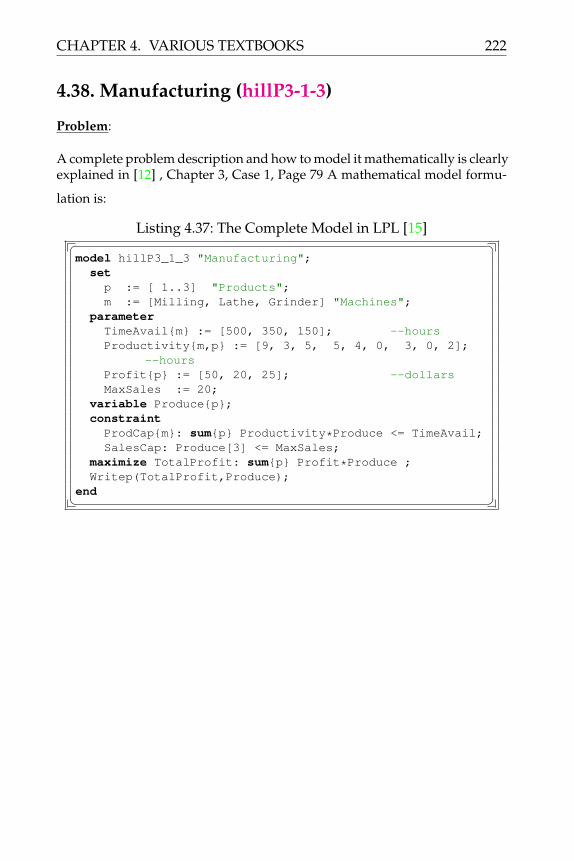
CHAPTER 4. VARIOUS TEXTBOOKS 222

4.38. Manufacturing (hillP3-1-3)

Problem:

A complete problem description and how to model it mathematically is clearlyexplained in [12] , Chapter 3, Case 1, Page 79 A mathematical model formu-

lation is:

Listing 4.37: The Complete Model in LPL [15]� �model hillP3_1_3 "Manufacturing";

setp := [ 1..3] "Products";m := [Milling, Lathe, Grinder] "Machines";

parameterTimeAvail{m} := [500, 350, 150]; --hoursProductivity{m,p} := [9, 3, 5, 5, 4, 0, 3, 0, 2];

--hoursProfit{p} := [50, 20, 25]; --dollarsMaxSales := 20;

variable Produce{p};constraintProdCap{m}: sum{p} Productivity*Produce <= TimeAvail;SalesCap: Produce[3] <= MaxSales;

maximize TotalProfit: sum{p} Profit*Produce ;Writep(TotalProfit,Produce);

end� �

223 CHAPTER 4. VARIOUS TEXTBOOKS

4.39. TV Manufacturing (hillP3-1-4)

Problem:

A complete problem description and how to model it mathematically is clearlyexplained in [12] , Chapter 3.1, Problem 4, Page 69 A mathematical model for-

mulation is:

Listing 4.38: The Complete Model in LPL [15]� �model hillP3_1_4 "TV Manufacturing";

set tvset := [i27, i20];parameterMaxDemand{tvset} := [40, 10];WorkHoursAvail := 500;WorkReq{tvset} := [20, 10];Profit{tvset} := [120, 80];

variable Produce{tvset} [0..MaxDemand];constraintWorkLimit: sum{tvset} WorkReq*Produce <=

WorkHoursAvail;maximize TotalProfit: sum{tvset} Profit*Produce ;Writep(TotalProfit,Produce);

end� �

CHAPTER 4. VARIOUS TEXTBOOKS 224

4.40. Resource PQ (hillP3-1-5)

Problem:

A complete problem description and how to model it mathematically is clearlyexplained in [12] , Chapter 3.1, Problem 5, Page 69 A mathematical model for-

mulation is:

Listing 4.39: The Complete Model in LPL [15]� �model hillP3_1_5 "Resource PQ";

setproduct := [1..2];resource := [P, Q];

parameterResourceReq{product,resource} := [1, 2, 3, 2];Profit{product} := [1, 2];ResourceAvail{resource} := [200, 300];MaxProduce2 := 60;

variable Produce{product};constraintResourceLimit{resource}: sum{product} ResourceReq*

Produce <= ResourceAvail;ProduceLimit: Produce[2] <= MaxProduce2;

maximize TotalProfit: sum{product} Profit*Produce ;Writep(TotalProfit,Produce);

end� �

225 CHAPTER 4. VARIOUS TEXTBOOKS

4.41. Insurance (hillP3-1-6)

Problem:

A complete problem description and how to model it mathematically is clearlyexplained in [12] , Chapter 3.1, Problem 6, Page 70 A mathematical model for-

mulation is:

Listing 4.40: The Complete Model in LPL [15]� �model hillP3_1_6 "Insurance";

setp := [SpecialRisk, Mortage] "product";d := [Underwriting, Administration, Claims] "

department";parameterProfit{p} := [5, 2];HoursAvail{d} := [2400, 800, 1200];HoursUnit{p, d} := [3, 0, 2, 2, 1, 0];

variable Produce{p};constraint WorkReq{d}: sum{p} HoursUnit*Produce <=

HoursAvail;maximize TotalProfit: sum{p} Profit*Produce ;Writep(TotalProfit,Produce);

end� �

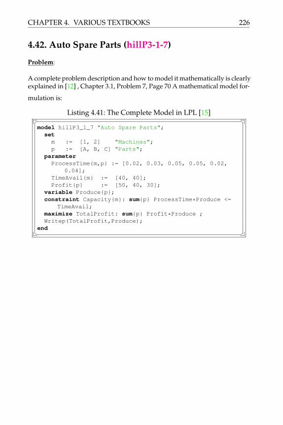
CHAPTER 4. VARIOUS TEXTBOOKS 226

4.42. Auto Spare Parts (hillP3-1-7)

Problem:

A complete problem description and how to model it mathematically is clearlyexplained in [12] , Chapter 3.1, Problem 7, Page 70 A mathematical model for-

mulation is:

Listing 4.41: The Complete Model in LPL [15]� �model hillP3_1_7 "Auto Spare Parts";

setm := [1, 2] "Machines";p := [A, B, C] "Parts";

parameterProcessTime{m,p} := [0.02, 0.03, 0.05, 0.05, 0.02,

0.04];TimeAvail{m} := [40, 40];Profit{p} := [50, 40, 30];

variable Produce{p};constraint Capacity{m}: sum{p} ProcessTime*Produce <=

TimeAvail;maximize TotalProfit: sum{p} Profit*Produce ;Writep(TotalProfit,Produce);

end� �

227 CHAPTER 4. VARIOUS TEXTBOOKS

4.43. Resource QRS (hillP3-2-1)

Problem:

A complete problem description and how to model it mathematically is clearlyexplained in [12] , Chapter 3.2, Problem 1, Page 71 A mathematical model for-

mulation is:

Listing 4.42: The Complete Model in LPL [15]� �model hillP3_2_1 "Resource QRS";

setp := [A, B] "Products";r := [Q, R, S] "Resources";

parameterProfit{p} := [3, 2];ResAvail{r} := [2, 2, 4];ResUsed{p,r}:= [2, 1, 3, 1, 2, 3];

variable Produce{p};constraint Capacity{r}: sum{p} ResUsed*Produce <=

ResAvail;maximize TotalProfit: sum{p} Profit*Produce ;Writep(TotalProfit,Produce);

end� �

CHAPTER 4. VARIOUS TEXTBOOKS 228

4.44. Invest Venture (hillP3-2-3)

Problem:

A complete problem description and how to model it mathematically is clearlyexplained in [12] , Chapter 3.2, Problem 3, Page 72 A mathematical model for-

mulation is:

Listing 4.43: The Complete Model in LPL [15]� �model hillP3_2_3 "Invest Venture";

set v := [1..2] "Ventures";parameterCashOnHand := 6000;InvestCash{v} := [5000, 4000];WorkReq{v} := [400, 500];Profit{v} := [4500, 4500];WorkHoursAvail:= 600;

variable InvestShare{v} [0..1];constraintCashLimit: sum{v} InvestCash*InvestShare <=

CashOnHand;WorkLimit: sum{v} WorkReq*InvestShare <=

WorkHoursAvail;maximize TotalProfit: sum{v} Profit*InvestShare ;Writep(TotalProfit,InvestShare);

end� �

229 CHAPTER 4. VARIOUS TEXTBOOKS

4.45. Investment (hillP3-4-10)

Problem:

A complete problem description and how to model it mathematically is clearlyexplained in [12] , Chapter 3.4, Problem 10, Page 76 A mathematical model

formulation is:

Listing 4.44: The Complete Model in LPL [15]� �model hillP3_4_10 "Investment";

seta := [1, 2, 3] "assets";y := [5, 10, 20] "years";

parameterAssetCost := 100;AssetIncome{a,y}:= [200, 50, 0, 100, 50, 150,

50, 100, 200];MinCashFlowReq{y} := [4000, 0, 3000];

variable Invest{a};constraint Requirement{y}: sum{a} AssetIncome*Invest >=

MinCashFlowReq;minimize TotalAmount: sum{a} AssetCost*Invest ;Writep(TotalAmount,Invest);

end� �

CHAPTER 4. VARIOUS TEXTBOOKS 230

4.46. Investor ABCD (hillP3-4-11)

Problem:

A complete problem description and how to model it mathematically is clearlyexplained in [12] , Chapter 3.4, Problem 11, Page 76 A mathematical model

formulation is:

Listing 4.45: The Complete Model in LPL [15]� �model hillP3_4_11 "Investor ABCD";

seti := [A, B, C, D] "investments";y :=[ 1..5] "years";InvestAvail{i,y} :=

[A 1, A 2, A 3, A 4, B 1, B 2, B 3, C 2, D 5];parameterTotalInvest := 60000;InvestReturn{i} := [1.40, 1.70, 1.90, 1.30];

variableMakeInvest,I{i,y|InvestAvail};MoneyAvailEnd,M{y};

constraintMoneyBalance{y}: M = if(y=1,TotalInvest,M[y-1])

+ sum{i} InvestReturn*I[(#y-2+y)%#y+1] - sum{i} I;MoneyLimit{y}: sum{i} I <= if(y=1,TotalInvest,M[y-1])

;maximize MoneyAccumulated: MoneyAvailEnd[#y];Writep(MoneyAccumulated,I,M);

end� �

231 CHAPTER 4. VARIOUS TEXTBOOKS

4.47. Alloy Blending (hillP3-4-12)

Problem:

A complete problem description and how to model it mathematically is clearlyexplained in [12] , Chapter 3.4, Problem 12, Page 76 A mathematical model

formulation is:

Listing 4.46: The Complete Model in LPL [15]� �model hillP3_4_12 "Alloy Blending";

seta := [1..5] "alloy";e := [Tin, Zinc, Lead] "elements";

parameterNewAlloyReq{e} := [40, 35, 25];ElementPct{e,a}:= [60, 25, 45, 20, 50,

10, 15, 45, 50, 40,30, 60, 10, 30, 10];

AlloyCost{a} := [22, 20, 25, 24, 27];variable Blend{a};constraint BlendReq{e}: sum{a} ElementPct*Blend >=

NewAlloyReq;minimize TotalCost: sum{a} AlloyCost*Blend ;Writep(TotalCost,Blend);

end� �

CHAPTER 4. VARIOUS TEXTBOOKS 232

4.48. Computer Fac Oper Assignment (hillP3-4-13)

Problem:

A complete problem description and how to model it mathematically is clearlyexplained in [12] , Chapter 3.4, Problem 13, Page 76 A mathematical model

formulation is:

Listing 4.47: The Complete Model in LPL [15]� �model hillP3_4_13 "Computer Fac Oper Assignment";

setw := [Mon, Tues, Wed, Thurs, Fri] "Workdays";o := [KC, DH, HB, SC, KS, NK] "Operators";Male{o} := [KC, DH, HB, SC] "Males";Female{o} := [KS, NK] "Females";

parameterWageRate{o} := [10.00, 10.10, 9.90, 9.80, 10.80,

11.30];HoursAvail{o,w} := [6, 0, 6, 0, 6,

0, 6, 0, 6, 0,4, 8, 4, 0, 4,5, 5, 5, 0, 5,3, 0, 3, 8, 0,0, 0, 0, 6, 2];

variable AssignHours{o,w|HoursAvail>0} [0..HoursAvail];constraintAssignDay{w}: sum{o} AssignHours >= 14;MinHours{Male}: sum{w} AssignHours >= if(Male,8,7);

minimize TotalCost: sum{o,w} WageRate*AssignHours;Writep(TotalCost,AssignHours);

end� �

233 CHAPTER 4. VARIOUS TEXTBOOKS

4.49. Warehouse Storage (hillP3-4-14)

Problem:

A complete problem description and how to model it mathematically is clearlyexplained in [12] , Chapter 3.4, Problem 14, Page 77 A mathematical model

formulation is:

Listing 4.48: The Complete Model in LPL [15]� �model hillP3_4_14 "Warehouse Storage";

setm,m1 := [ 1..5] "Months";p := [ 1..5] "Periods";

parameterSpaceReq{m} :=[30 20 40 10 50]; -- 1000sfLeaseCost{p}:=[650 1000 1350 1600 1900]; -- $00/1000

sfvariable SpaceLeased{m,p|p<=6-m};constraint MinSpace{m1}: sum{m,p|m<=m1 and p>m1-m}

SpaceLeased >= SpaceReq;minimize TotalCost: sum{m,p} LeaseCost*SpaceLeased;Writep(TotalCost,SpaceLeased);

end� �

CHAPTER 4. VARIOUS TEXTBOOKS 234

4.50. Paper Manufacturing (hillP3-4-15)

Problem:

A complete problem description and how to model it mathematically is clearlyexplained in [12] , Chapter 3.4, Problem 15, Page 78 A mathematical model

formulation is:

Listing 4.49: The Complete Model in LPL [15]� �model hillP3_4_15 "Paper Manufacturing";

setmill,i := [p1,p2,p3,p4];machine,m := [m1,m2,m3];rawmat,r := [r1,r2,r3,r4];papertype,p := [t1,t2,t3,t4,t5];customer,c := [c1,c2,c3,c4,c5,c6,c7,c8];

parameterPaperDemand{c,p} := Rnd(1,20);RawMatUsed{p,m,r} := Rnd(1,4);RawMatAvail{i,r} := Rnd(100,1000);MachineUse{p,m} := Rnd(1,4);MachineAvail{i,m} := Rnd(100,1000);ProduceCost{i,p,m} := Rnd(1,10);TransportCost{i,c,p} := Rnd(1,10);

variableProduce,P{i,m,p|ProduceCost};Ship,S{i,c,p|TransportCost};

constraintRawMat{i,r}: sum{m,p} RawMatUsed*P <= RawMatAvail;ProdCap{i,m}: sum{p} MachineUse*P <= MachineAvail;MillBalance{i,p}: sum{m} P = sum{c} S;MeetDemand{c,p}: sum{i} S >= PaperDemand;

minimize TotalCost: sum{i,m,p} ProduceCost*P + sum{i,c,p} TransportCost*S;

Writep(TotalCost,P,S);end� �

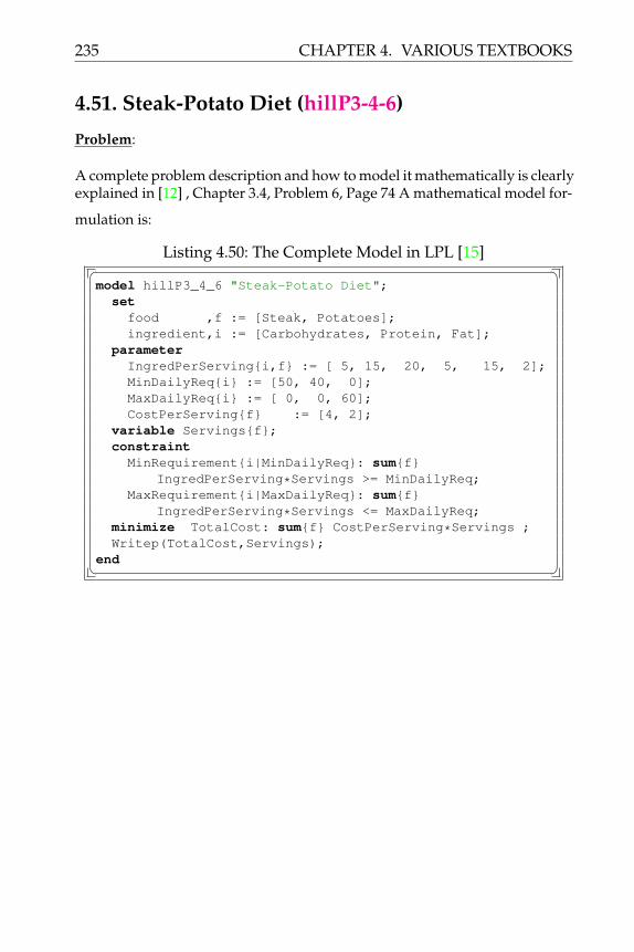
235 CHAPTER 4. VARIOUS TEXTBOOKS

4.51. Steak-Potato Diet (hillP3-4-6)

Problem:

A complete problem description and how to model it mathematically is clearlyexplained in [12] , Chapter 3.4, Problem 6, Page 74 A mathematical model for-

mulation is:

Listing 4.50: The Complete Model in LPL [15]� �model hillP3_4_6 "Steak-Potato Diet";

setfood ,f := [Steak, Potatoes];ingredient,i := [Carbohydrates, Protein, Fat];

parameterIngredPerServing{i,f} := [ 5, 15, 20, 5, 15, 2];MinDailyReq{i} := [50, 40, 0];MaxDailyReq{i} := [ 0, 0, 60];CostPerServing{f} := [4, 2];

variable Servings{f};constraintMinRequirement{i|MinDailyReq}: sum{f}

IngredPerServing*Servings >= MinDailyReq;MaxRequirement{i|MaxDailyReq}: sum{f}

IngredPerServing*Servings <= MaxDailyReq;minimize TotalCost: sum{f} CostPerServing*Servings ;Writep(TotalCost,Servings);

end� �

CHAPTER 4. VARIOUS TEXTBOOKS 236

4.52. Pig Feed Blending (hillP3-4-7)

Problem:

A complete problem description and how to model it mathematically is clearlyexplained in [12] , Chapter 3.4, Problem 7, Page 74 A mathematical model for-

mulation is:

Listing 4.51: The Complete Model in LPL [15]� �model hillP3_4_7 "Pig Feed Blending";

setf := [Corn, Tankage, Alfalfa] "feed";i := [Carbohydrates, Protein, Vitamins] "ingredient";

parameterIngredient{f, i}:=[90 30 10, 20 80 20, 40 60 60];MinDailyReq{i} :=[200, 180, 150];Cost{f} :=[0.84, 0.72, 0.60];

variable FeedUse,F{f};constraint Requirement{i}: sum{f} Ingredient*F >=

MinDailyReq;minimize TotalCost: sum{f} Cost*F;Writep(TotalCost,F);

end� �

237 CHAPTER 4. VARIOUS TEXTBOOKS

4.53. Plant Production Planning (hillP3-4-8)

Problem:

A complete problem description and how to model it mathematically is clearlyexplained in [12] , Chapter 3.4, Problem 8, Page 75 A mathematical model for-

mulation is:

Listing 4.52: The Complete Model in LPL [15]� �model hillP3_4_8 "Plant Production Planning";

setplant ,p := [1..3];size ,s := [Large, Medium, Small];

parameterProfit{s} := [420, 360, 300];PlantCapacity{p} := [750, 900, 450];SpaceAvail{p} := [13000, 12000, 5000];SpaceReq{s} := [20, 15, 12];Demand{s} := [900, 1200, 750];

variable Produce{p,s};constraintCapacityLimit{p}: sum{s} Produce <= PlantCapacity;SpaceLimit{p}: sum{s} SpaceReq*Produce <= SpaceAvail;MaxDemand{s}: sum{p} Produce <= Demand;EqualCapUse{p|p<#p}: 1/PlantCapacity*(sum{s} Produce)

= 1/PlantCapacity[p+1]*(sum{s} Produce[p+1,s]);maximize TotalProfit: sum{p,s} Profit*Produce ;Writep(TotalProfit,Produce);

end� �

CHAPTER 4. VARIOUS TEXTBOOKS 238

4.54. Cargo Plane Planning (hillP3-4-9)

Problem:

A complete problem description and how to model it mathematically is clearlyexplained in [12] , Chapter 3.4, Problem 9, Page 75 A mathematical model for-

mulation is:

Listing 4.53: The Complete Model in LPL [15]� �model hillP3_4_9 "Cargo Plane Planning";

setc := [Front, Center, Back] "compartment";g :=[ 1..4] "cargo";

parameterWeightCapacity{c} := [12, 18, 10];SpaceCapacity{c} := [7000, 9000, 5000];CargoAvail{g} := [20, 16, 25, 13];Volume{g} := [500, 700, 600, 400];Profit{g} := [320, 400, 360, 290];

variable AcceptCargo{c,g};constraintCargoLimit{g}: sum{c} AcceptCargo <= CargoAvail;WeightLimit{c}: sum{g} AcceptCargo <= WeightCapacity;SpaceLimit{c}: sum{g} Volume*AcceptCargo <=

SpaceCapacity;maximize TotalProfit: sum{c,g} Profit*AcceptCargo;Writep(TotalProfit,AcceptCargo);

end� �

239 CHAPTER 4. VARIOUS TEXTBOOKS

4.55. MidWest Grain Elevator (midwest)

Problem:

Midwest Grain Elevator: Case Summary Statement: Midwest Grain Elevatorperforms storage and handling services for buyers and sellers of grain on aservice fee basis. To achieve maximum profit Midwest must maximize theamount of grain it handles. In order to accomplish this objective, Midwestmust build customer loyalty on the part of both buyers and sellers of grain.Thus, Midwest’s preferred policy is to encourage repeat business by satisfyingbuyers’ orders at minimum cost. This policy benefits sellers as well as byincreasing the number of orders for high quality grain that can be filled.

Currently Midwest is storing 507,900 bushels of corn for Saw Mill River Feed& Grain Company. This corn has been classified into 26 different types, whichdiffer by moisture content, weight per bushel, amount of damage, and amountof foreign material. Saw Mill has limited quantities of each of the 26 types ofcorn. The ability to meet an order is obviously restricted by this supply. Thequantities and cost of each type of corn is detailed in the table shown below.Corn Cost and Supply Table

Corn Type Supply Cost--------------------------------------

1 15000 1.502 30000 1.453 45000 1.444 25000 1.455 40000 1.426 20000 1.387 30000 1.378 75000 1.379 15000 1.3910 50000 1.3911 16000 1.2712 20000 1.2813 10000 1.1714 12000 1.2215 6000 1.1216 2000 1.1817 5000 1.4218 4000 1.4219 5000 1.4220 6000 1.3621 1300 1.2922 29000 1.2923 1900 1.42

CHAPTER 4. VARIOUS TEXTBOOKS 240

24 33000 1.4025 6700 1.2226 5000 1.30

--------------------------------------

Saw Mill has now received an order for 6 different grades of corn totaling

1. bushels which it intends to fill from the grain stored with Midwest. TheSaw Mill must meet the stated demand for each of the 6 grades. Exceed-ing demand would be ill-advised, since there is no guarantee that thenext order filled will require the same characteristics. The demand foreach type of grade is shown in the table below.

Corn Grade Demand-------------------------

Gr1 40000Gr2 32000Gr3 50000Gr4 20000Gr5 30000Gr6 100000

-------------------------

Midwest’s handling fee will be based on supplying the 272,000 bushelsof corn, regardless of the manner in which the various corns are blendedto meet the specifications. However, in keeping with the policy of pro-viding quality service to other buyers and sellers, the problem Mid-west faces is that of determining the least cost blend of available grainsthat will satisfy the specified criteria of the current order. Each of the6 grades of corn demanded must meet specified criteria for moisturecontent, minimum weight per bushel, percentage damaged, and per-centage of foreign material, which are detailed in the table below. CornGrade Characteristics:

Grade MaxMoisture MinWeight MaxDamage MaxForeign---------------------------------------------------------

Gr1 13.0 56.0 2.0 2.0Gr2 15.5 54.0 5.0 3.0Gr3 15.0 56.0 2.0 4.0Gr4 16.0 54.0 9.0 4.0Gr5 23.0 54.0 10.0 6.0Gr6 20.0 54.0 9.0 4.0

---------------------------------------------------------

For each of the 6 grades the four quality requirements are as follows:The weighted average moisture content cannot exceed the maximumacceptable moisture level for that grade. The weighted average weightper bushel of the corns used in the blend of the grades must meet or

241 CHAPTER 4. VARIOUS TEXTBOOKS

exceed the minimum level. The weighted average percent damagedof the 26 types of corn used in the blend cannot exceed the maximumlevel. The weighted average percentage of foreign material that couldbe used in the blend cannot exceed the maximum requirement. Thequality characteristics for each of the 26 corn types is given in the tablebelow. Corn Quality Characteristics:

Corn Type Moisture Weight Damage Foreign------------------------------------------------------

1 11.0 58.0 3.0 1.02 12.0 57.0 2.0 1.53 15.0 57.0 2.0 1.04 12.0 58.0 3.0 3.05 13.0 56.0 4.0 2.06 15.0 54.0 4.0 2.07 15.0 55.0 5.0 3.08 18.0 57.0 5.0 1.09 14.0 58.0 2.0 4.010 15.0 55.0 3.0 2.011 17.0 53.0 7.0 5.012 15.0 55.0 8.0 3.013 22.0 56.0 8.0 5.014 18.0 54.0 13.0 5.015 17.0 55.0 20.0 8.016 13.5 57.0 30.0 2.017 13.5 57.0 3.0 2.018 13.5 57.5 3.0 2.019 13.5 57.0 5.0 3.020 15.0 56.5 10.0 4.021 13.5 58.0 15.0 4.022 13.0 57.0 15.0 5.023 13.0 58.0 3.0 2.024 13.0 56.0 5.0 3.025 14.0 56.0 20.0 5.026 15.0 56.5 10.0 4.0

-------------------------------------------------------

The objective for this problem is to determine the number of bushels usedin the blending for each of the 26 types of corn so the the total cost of the 6desired grades of corn is minimized.

Reference: Prof. Ramesh Sharda, Operations Research Dept., Oklahoma StateUniversity

Modeling Steps

CHAPTER 4. VARIOUS TEXTBOOKS 242

Listing 4.54: The Complete Model in LPL [15]

� �model midwest "MidWest Grain Elevator";

settype := [1..26];grade := [Gr1, Gr2, Gr3, Gr4, Gr5, Gr6];

parameter-- Supply characteristicsSupply{type} := [15000, 30000, 45000, 25000, 40000,

20000, 30000, 75000, 15000,50000, 16000, 20000, 10000, 12000, 6000, 2000,

5000, 4000, 5000, 6000, 1300, 29000, 1900,33000, 6700, 5000];

Cost{type} := [1.50, 1.45, 1.44, 1.45, 1.42, 1.38,1.37, 1.37, 1.39

1.39, 1.27, 1.28, 1.17, 1.22, 1.12, 1.18, 1.42, 1.421.42, 1.36, 1.29, 1.29, 1.42, 1.40, 1.22, 1.30 ];

Moisture{type} := [11, 12, 15, 12, 13, 15, 15, 18,14,

15, 17, 15, 22, 18, 17, 13.5, 13.5 13.5,13.5, 15, 13.5, 13, 13, 13, 14, 15];

Weight{type} := [58.0, 57.0, 57.0, 58.0, 56.0, 54.0,55.0, 57.0, 58.0,

55.0, 53.0, 55.0, 56.0, 54.0, 55.0, 57.0, 57.0,57.5,

57.0, 56.5, 58.0, 57.0, 58.0, 56.0, 56.0, 56.5];Damage{type} := [ 3, 2, 2, 3, 4, 4, 5, 5, 2,

3, 7, 8, 8, 13, 20, 30, 3, 3,5, 10, 15, 15, 3, 5, 20, 10];

Foreign {type} := [1, 1.5, 1, 3, 2, 2, 3, 1, 4,2, 5, 3, 5, 5, 8, 2, 2, 2,3, 4, 4, 5, 2, 3, 5, 4];

-- Demand CharacteristicsDemand{grade} := [40000, 32000, 50000, 20000, 30000,

100000];MaxMoisture{grade} := [13, 115, 15, 16, 23, 20];MinWeight{grade} := [56, 54, 56, 54, 54, 54];MaxDamage{grade} := [2, 5, 2, 9, 10, 9];MaxForeign{grade} := [2, 3, 4, 4, 6, 4];

variable Bushels{type,grade};constraintQuantitySupplied{type}: sum{grade} Bushels <= Supply;QuantityDemanded{grade}: sum{type} Bushels = Demand;MoistureContent{grade}: sum{type} Moisture*Bushels <=

MaxMoisture*(sum{type} Bushels);WeightPerBushel{grade}: sum{type} Weight*Bushels >=

MinWeight*(sum{type} Bushels);DamagePercent{grade}: sum{type} Damage*Bushels <=

MaxDamage*(sum{type} Bushels);

243 CHAPTER 4. VARIOUS TEXTBOOKS

ForeignMaterial{grade}: sum{type} Foreign*Bushels <=MaxForeign*(sum{type} Bushels);

minimize totalcost: sum{type,grade} Cost*Bushels;Writep(totalcost,Bushels);

end� �Solution:

opt: 366863;

CHAPTER 4. VARIOUS TEXTBOOKS 244

4.56. Fertilizer (murty2-1)

Problem:

A complete problem description and how to model it mathematically is clearlyexplained in [18], Example 2.1, Page 23 A mathematical model formulation is:

Listing 4.55: The Complete Model in LPL [15]� �model murty2_1 "Fertilizer";

setfertilizer,f := ['Hi-ph', 'Lo-ph'];material ,m := [RM1, RM2, RM3];

parameterNetProfit{f} := [15, 10];RawMatReq{f,m} := [2, 1, 1, 1, 1, 0];RawMatAvail{m} := [1500, 1200, 500];

variable Produce{f};constraint Req{m}: sum{f} RawMatReq*Produce <=

RawMatAvail;maximize TotalProfit: sum{f} NetProfit*Produce;Writep(TotalProfit,Produce);

end� �

245 CHAPTER 4. VARIOUS TEXTBOOKS

4.57. Gasoline Blending (murty2-2)

Problem:

A complete problem description and how to model it mathematically is clearlyexplained in [18], Example 2.2, Page 28 A mathematical model formulation is:

Listing 4.56: The Complete Model in LPL [15]� �model murty2_2 "Gasoline Blending";

setrawgas,r := [1..4];fueltype,f := [1..3];

parameterOctaneRating{r} := [68, 86, 91, 99];RawGasAvail{r} := [4000, 5050, 7100, 4300];RawGasCost{r} := [31.02, 33.15, 36.35, 38.75];RawGasPrice{r} := [36.85, 36.85, 38.95, 38.95];MinOctaneFuel{f} := [95, 90, 85];FuelPrice{f} := [45.15, 42.95, 40.99];MinimumDemand{f} := [0, 0, 15000];MaximumDemand{f} := [10000, 0, 0];

variableFuelComposition,FC{f,r};RawGasSold,RG{r};

expressionTotalFuelRevenue : sum{r,f} FuelPrice*FC;TotalRawGasRevenue: sum{r} RawGasPrice*RG;TotalRawGasCost : sum{r,f} RawGasCost*FC + sum{r}

RawGasCost*RG;constraintRawGasLimit{r}: sum{f} FC + RG <= RawGasAvail;OctaneReq{f}: sum{r} OctaneRating*FC >= MinOctaneFuel

*(sum{r} FC);MinDemand{f|MinimumDemand}: MinimumDemand <= sum{r}

FC;MaxDemand{f|MaximumDemand}: sum{r} FC <=

MaximumDemand;maximize TotalProfit: TotalFuelRevenue +

TotalRawGasRevenue - TotalRawGasCost;Writep(TotalProfit,FC,RG);

end� �

CHAPTER 4. VARIOUS TEXTBOOKS 246

4.58. Diet Problem (murty2-3)

Problem:

A complete problem description and how to model it mathematically is clearlyexplained in [18], Example 2.3, Page 31 A mathematical model formulation is:

Listing 4.57: The Complete Model in LPL [15]� �model murty2_3 "Diet Problem";

setgrain := [1..2];nutri := [Starch, Protein, Vitamins];

parameterNutriUnits{nutri,grain} := [5, 7, 4, 2, 2, 1];MinDailyReq{nutri} := [8, 15, 3];GrainCost{grain} := [0.60, 0.35];

variable Amount{grain};constraintRequirement{nutri}: sum{grain} NutriUnits*Amount >=

MinDailyReq;minimize TotalCost: sum{grain} GrainCost*Amount;Writep(TotalCost,Amount);

end� �

247 CHAPTER 4. VARIOUS TEXTBOOKS

4.59. Transportation (murty2-4)

Problem:

A complete problem description and how to model it mathematically is clearlyexplained in [18],Example 2.4, Page 33 A mathematical model formulation is:

Listing 4.58: The Complete Model in LPL [15]� �model murty2_4 "Transportation";

setmine := [1..2];plant := [1..3];

parameterAvailability{mine} := [800, 300];Requirement{plant} := [400, 500, 200];ShipCost{mine,plant} := [11, 8, 2, 7, 5, 4];

variable Ship{mine,plant};constraintOreLimit{mine}: sum{plant} Ship <= Availability;OreReq{plant}: sum{mine} Ship >= Requirement;

minimize TotalCost: sum{mine,plant} ShipCost*Ship;Writep(TotalCost,Ship);

end� �

CHAPTER 4. VARIOUS TEXTBOOKS 248

4.60. Marriage Problem (murty2-5)

Problem:

A complete problem description and how to model it mathematically is clearlyexplained in [18],Example 2.5, Page 36 A mathematical model formulation is:

Listing 4.59: The Complete Model in LPL [15]� �model murty2_5 "Marriage Problem";

setman := [1..5];woman := [1..5];

parameterHappyness{man,woman} := [ 78, -16, 19, 25, 83,

99, 98, 87, 16, 92,86, 19, 39, 88, 17,

-20, 99, 88, 79, 65,67, 98, 90, 48, 60];

variable TimeTogether{man,woman};constraintMenMonogamous{man}: sum{woman} TimeTogether = 1;WomenMonogamous{woman}: sum{man} TimeTogether = 1;

maximize TotalHappyness: sum{man,woman} Happyness*TimeTogether;

Writep(TotalHappyness,TimeTogether);end� �

249 CHAPTER 4. VARIOUS TEXTBOOKS

4.61. Multi-Period Planning (murty2-6)

Problem:

A complete problem description and how to model it mathematically is clearlyexplained in [18], Example 2.6, Page 40 A mathematical model formulation is:

Listing 4.60: The Complete Model in LPL [15]� �model murty2_6 "Multi-Period Planning";

set period,p := [1..6];parameterProdCost{p} := [20, 25, 30, 40, 50, 60];ProdCapacity{p}:= [1500 2000 2200 3000 2700 2500];Demand{p} := [1100 1500 1800 1600 2300 2500];SellingPrice{p}:= [180, 180, 250, 270, 300, 320];InventoryCost := 2;InitialStock := 500;FinalStock := 500;

variableProduce,P{p} [0..ProdCapacity];Inventory,I{p};Sales,S{p} [0..Demand];

expressionTotalRevenue : sum{p} SellingPrice*S;TotalProdCost: sum{p} ProdCost*P;TotalInvtCost: sum{p} InventoryCost*I;TotalCost : TotalProdCost + TotalInvtCost;

constraintInventoryBalance{p}: I = if(p=1,InitialStock,I[p-1])

+ P - S;F: I[6] = FinalStock;

maximize NetProfit: TotalRevenue - TotalCost;Writep(NetProfit,P,I,S);

end� �

CHAPTER 4. VARIOUS TEXTBOOKS 250

4.62. Breck and Dapper (shapiro1-1)

Problem:

A complete problem description and how to model it mathematically is clearlyexplained in [23], Example 1.1, Page 12. A mathematical model formulation

is:

Listing 4.61: The Complete Model in LPL [15]� �model shapiro1_1 "Breck and Dapper";

set drill := [1..4];parameterPlastReq{drill} := [0.82, 0.62, 1.42, 2.03]; -- lbCopperReq{drill} := [0.43, 0.69, 0.33, 0.20]; -- lbWireReq{drill} := [15, 16, 9, 9]; -- ydContrib{drill} := [12.5 11.3 17.2 19.9]; -- dollarsPlastAvail := 16000; -- lbCopperAvail := 5000; -- lbWireOnHand := 8000; -- ydProdWireCap := 80000; -- ydProdWireRate := 3.6/100; -- lb/ydWireProdCost := 0.14;WirePurchaseCost := 0.29;

variableProduce,x{drill};WirePurchase,Wp;WireProduce,Wm [0..ProdWireCap];

constraintPlastLimit: sum{drill} PlastReq*x <= PlastAvail;CopperLimit: sum{drill} CopperReq*x + ProdWireRate*Wm

<= CopperAvail;WireLimit: sum{drill} WireReq*x <= WireOnHand + Wm +

Wp;Marketing: x[1] + x[2] >= x[3] + x[4];

maximize TotalProfit: sum{drill} Contrib*x -WireProdCost*Wm - WirePurchaseCost*Wp;

Writep(TotalProfit,x,Wp,Wm);end� �

251 CHAPTER 4. VARIOUS TEXTBOOKS

4.63. DowPont Chemical (shapiro1-2)

Problem:

A complete problem description and how to model it mathematically is clearlyexplained in [23], Example 1.2, Page 17. A mathematical model formulation

is:

Listing 4.62: The Complete Model in LPL [15]� �model shapiro1_2 "DowPont Chemical";

setchemical,c := [R,A,B,C,D];process,p := [1..3];

parameterRawMatCost := 1;ProcessCapacity{p} := [56, 25, 46];MarketPrice{c} := [0.00, 2.40, 3.20, 6.40, 12.20];ProcessCost{p,c} := /1 R 1.50, 2 A 3.50, 3 B 4.20, 3

C 4.20/;ProcessOutput{p,c} := /1 A 0.45, 1 B 0.55, 2 C 0.80,

3 D 0.75/;variableProdSale,S{c};ProdUse,U{c};

constraintr1: U['A']+S['A'] = ProcessOutput['1','A'] * U['R'];r2: U['B']+S['B'] = ProcessOutput['1','B'] * U['R'];r3: U['C']+S['C'] = ProcessOutput['2','C'] * U['A'];r4: S['D'] = ProcessOutput['3','D']*(U['B'] + U['C'])

;r5: U['B'] = 1.5*U['C'];r6: U['R'] <= ProcessCapacity['1'];r7: U['A'] <= ProcessCapacity['2'];r8: U['B'] + U['C'] <= ProcessCapacity['3'];

maximize TotalProfit:sum{c} MarketPrice*S - RawMatCost*U['R'] - sum{c,p}

ProcessCost*U;Writep(TotalProfit,S,U);

end� �

CHAPTER 4. VARIOUS TEXTBOOKS 252

4.64. Portfolio Selection (shapiro1-3)

Problem:

A complete problem description and how to model it mathematically is clearlyexplained in [23], Example 1.3, Page 21. A mathematical model formulation

is:

Listing 4.63: The Complete Model in LPL [15]� �model shapiro1_3 "Portfolio Selection";

setbond := [A, B, C, D, E];type := [Municipal, Agency, Government];BondType{bond,type} := [A Municipal,

B Agency,C Government,D Government,E Municipal];

parameterTotalAvailForInvest := 10;QualityBank{bond} := [2, 2, 1, 1, 5];YearsToMaturity{bond} := [9, 15, 4, 3, 2];Yield{bond} := [0.086, 0.108, 0.1, 0.088,

0.09];YieldAfterTax{bond} := [0.086, 0.054, 0.05, 0.044,

0.09];MaxMunicipal := 3;MaxAvgQuality := 1.4;MaxAvgMaturity := 5;TaxRate := 0.5;

variable Invest,x{bond};constraintAmountInvested: sum{bond} x <= TotalAvailForInvest;MaxInvestType{type|type='Municipal'}: sum{bond|

BondType} x <= MaxMunicipal;QualityReq: sum{bond} QualityBank*x <= MaxAvgQuality

*(sum{bond} x);MaturityReq: sum{bond} YearsToMaturity*x <=

MaxAvgMaturity*(sum{bond} x);maximize AfterTaxEarnings: sum{bond} YieldAfterTax*x;Writep(AfterTaxEarnings,x);

end� �

253 CHAPTER 4. VARIOUS TEXTBOOKS

4.65. Portfolio Selection (shapiro1-3b)

Problem:

A complete problem description and how to model it mathematically is clearlyexplained in [23], Example 1.3b, Page 21. A mathematical model formulation

is:

Listing 4.64: The Complete Model in LPL [15]� �model shapiro1_3b "Portfolio Selection";

set bond := [A, B, C, D, E];type := [Municipal, Agency, Government];BondType{bond,type} := [A Municipal,

B Agency,C Government,D Government,E Municipal];

parameterTotalAvailForInvest := 10;QualityBank{bond} := [2, 2, 1, 1, 5];YearsToMaturity{bond} := [9, 15, 4, 3, 2];Yield{bond} := [0.086 0.108 0.1 0.088 0.09];YieldAfterTax{bond} := [0.086 0.054 0.05 0.044 0.09];MaxMunicipal := 3;MaxAvgQuality := 1.4;MaxAvgMaturity := 5;TaxRate := 0.5;BorrowInterestRate := 0.11;

variableInvest,x{bond};Borrow,y;

constraintAmountInvested: sum{bond} x <= TotalAvailForInvest+y;MaxInvestType{type|type='Municipal'}: sum{bond|

BondType} x <= MaxMunicipal;QualityReq: sum{bond} QualityBank*x <= MaxAvgQuality

*(sum{bond} x);MaturityReq: sum{bond} YearsToMaturity*x <=

MaxAvgMaturity*(sum{bond} x);MaxBorrow: Borrow <= 1;

maximize AfterTaxEarnings: sum{bond} YieldAfterTax*x -BorrowInterestRate*TaxRate*y;

Writep(AfterTaxEarnings,x,y);end� �

CHAPTER 4. VARIOUS TEXTBOOKS 254

4.66. Transportation (shapiro1-4)

Problem:

A complete problem description and how to model it mathematically is clearlyexplained in [23], Example 1.4, Page 24. A mathematical model formulation

is:

Listing 4.65: The Complete Model in LPL [15]� �model shapiro1_4 "Transportation";

setmill := [1..2];market := [Northburg, Midburg, Southburg];

parameterWheatAvail := 50000;MillingCost{mill} := [0.13, 0.16];MarketDemand{market} := [10000, 15000, 25000];ShipCostMill{mill} := [0.31, 0.33];ShipCostMarket{market, mill} := [0.18, 0.25, 0.22,

0.23, 0.27, 0.19];variableShipMill{mill};ShipMarket{mill, market};

constraintWheatToMills: sum{mill} ShipMill = WheatAvail;MillBalance{mill}: ShipMill = sum{market} ShipMarket;MarketReq{market}: sum{mill} ShipMarket =

MarketDemand;maximize TotalCost:sum{mill} MillingCost*ShipMill+ sum{mill} ShipCostMill*ShipMill+ sum{mill,market} ShipCostMarket*ShipMarket;

Writep(TotalCost,ShipMill,ShipMarket);end� �

255 CHAPTER 4. VARIOUS TEXTBOOKS

4.67. Multi-Period Scheduling (shapiro1-5)

Problem:

A complete problem description and how to model it mathematically is clearlyexplained in [23], Example 1.5, Page 28. A mathematical model formulation

is:

Listing 4.66: The Complete Model in LPL [15]� �model shapiro1_5 "Multi-Period Scheduling";

set m,month := [1..12];parameterDemand{m} := [3800, 4100, 4700, 5900, 7200, 7900,

6700, 5100, 5300, 6400, 5800, 4800];ProductionCost := 100; InventoryCost := 7;LaborCost := 1600; HiringCost := 300;LayoffCost := 500; StockOutCost := 500;RecordersPerDay := 8; AssemblyCapacity:= 7000;MaxNewWorkers := 50; MaxLayoffPercent:= 0.1;InitInventory := 750; InitWorkforce := 500;

variableProduce,P{m};Inventory,I{m}; Ie "final Inventory";Workers,W{m}; Hired,H{m};LaidOff,L{m}; StockOut,S{m};

expressionTotalProductionCost: sum{m} ProductionCost*P ;TotalInventoryCost : sum{m} InventoryCost*1/2*(I+if(m

=#m,Ie,I[m+1]));TotalLaborCost : sum{m} LaborCost*W ;TotalHiringCost : sum{m} HiringCost*H ;TotalLayoffCost : sum{m} LayoffCost*L ;TotalStockOutCost : sum{m} StockOutCost*S ;

constraintInvBalance{m}: P+I-if(m=#m,Ie,I[m+1])+S = Demand;WorkforceLimit{m}: P <= RecordersPerDay*W;AssemblyLimit{m}: P <= AssemblyCapacity;WorkforceBalance{m}: W = if(m=1,InitWorkforce,W[m-1])

+ H - L;MaxHired{m}: H <= MaxNewWorkers;MaxLaidOff{m}: L <= MaxLayoffPercent * if(m=1,

InitWorkforce,W[m-1]);II: I[1] = InitInventory;

minimize TotalCost: TotalProductionCost +TotalInventoryCost

+ TotalLaborCost + TotalHiringCost + TotalLayoffCost+ TotalStockOutCost;

CHAPTER 4. VARIOUS TEXTBOOKS 256

Writep(TotalCost,P,I,W,H,L,S);end� �

257 CHAPTER 4. VARIOUS TEXTBOOKS

4.68. Giapetto Wood Carving (winst3-1-1)

Problem: “Giapetto’s Woodcarving, Inc., manufactures two types of woodentoys: soldiers and trains. A soldier sells for $27 and uses $10 worth of raw ma-terials. Each soldier that is manufactured increases Giapetto’s variable laborand overhead costs by $14. A train sells for $21 and uses $9 worth of raw ma-terials. Each train built increases Giapetto’s variable labor and overhead costsby $10. The manufacture of wooden soldiers and trains requires two types ofskilled labor: carpentry and finishing. A soldier requires 2 hours of finishinglabor and 1 hour of carpentry labor. A train requires 1 hour of finishing and1 hour of carpentry labor. Each week, Giapetto can obtain all the needed rawmaterial but only 100 finishing hours and 80 carpentry hours. Demand fortrains is unlimited, but at most 40 soldiers are bought each week. Giapettowants to maximize weekly profit (revenues - costs). Formulate a mathemat-ical model of Giapetto’s situation that can be used to maximize Giapetto’sweekly profit.”This problem is from [30] , Example 3.1-1, Page 45.

Modeling Steps

Listing 4.67: The Complete Model in LPL [15]� �model winst3_1_1 "Giapetto Wood Carving";

sett := [Soldier, Train] "Toys";w := [Carpentry, Finishing] "Labor";

parameterPrice{t} := [27, 21];VariableCost{t} := [14, 10];RawMatCost{t} := [10, 9];Profit{t} := Price - VariableCost - RawMatCost;LaborHours{t,w} := [1, 2, 1, 1];LaborAvail{w} := [80, 100];MaxSoldier := 40;

variable Produce,P{t};constraintLaborCapacity{w} : sum{t} LaborHours*P <= LaborAvail;MaxDemand: P['Soldier'] <= MaxSoldier;

maximize TotalProfit : sum{t} Profit*P;Writep(TotalProfit,P);

end� �

CHAPTER 4. VARIOUS TEXTBOOKS 258

4.69. Giapetto Wood Carving II (winst3-1-1s)

Problem: “Giapetto’s Woodcarving, Inc., manufactures two types of woodentoys: soldiers and trains. A soldier sells for $27 and uses $10 worth of raw ma-terials. Each soldier that is manufactured increases Giapetto’s variable laborand overhead costs by $14. A train sells for $21 and uses $9 worth of raw ma-terials. Each train built increases Giapetto’s variable labor and overhead costsby $10. The manufacture of wooden soldiers and trains requires two types ofskilled labor: carpentry and finishing. A soldier requires 2 hours of finishinglabor and 1 hour of carpentry labor. A train requires 1 hour of finishing and1 hour of carpentry labor. Each week, Giapetto can obtain all the needed rawmaterial but only 100 finishing hours and 80 carpentry hours. Demand fortrains is unlimited, but at most 40 soldiers are bought each week. Giapettowants to maximize weekly profit (revenues - costs). Formulate a mathemat-ical model of Giapetto’s situation that can be used to maximize Giapetto’sweekly profit.”This problem is from [30] , Example 3.1-1, Page 45.

Modeling Steps

Listing 4.68: The Complete Model in LPL [15]� �model winst3_1_1s "Giapetto Wood Carving II";

variable soldier; train;constraintcarpentry: 1*soldier + 1*train <= 80;finishing: 2*soldier + 1*train <= 100;maxsoldier: soldier <=40;

maximize Profit: 27*soldier + 21*train - 24*soldier -19*train;

Writep(Profit);end� �

259 CHAPTER 4. VARIOUS TEXTBOOKS

4.70. Dorian Advertising (winst3-2-2)

Problem: ”Dorian Auto manufactures luxury cars and trucks. The companybelieves that its most likely customers are high-income women and men. Toreach these groups, Dorian Auto has embarked on an ambitious TV advertis-ing campaign and has decided to purchase 1-minute commercial spots on twotypes of programs: comedy shows and football games. Each comedy com-mercial is seen by 7 million high-income women and 2 million high-incomemen. Each football commercial is seen by 2 million high-income women and12 million high-income men. A 1-minute comedy ad costs $50,000, and a 1-minute football ad costs $100,000. Dorian would like the commercials to beseen by at least 28 million high-income women and 24 million high-incomemen. Use linear programming to determine how Dorian Auto can meet itsadvertising requirements at minimum cost.” This probelm is from [30] , Ex-ample 3.2-2, Page 57.

Modeling Steps

Listing 4.69: The Complete Model in LPL [15]� �model winst3_2_2 "Dorian Advertising";

seta := [Comedy, Football] "adtype";c := [HIW, HIM] "customers";

parameterMinuteCost{a} := [50, 100];SeenBy{a,c} := [7, 2, 2, 12];TargetReach{c} := [28, 24];

variable Purchase{a};constraintMustReach{c}: sum{a} SeenBy*Purchase >= TargetReach;

minimize TotalCost: sum{a} MinuteCost*Purchase ;Writep(TotalCost,Purchase);

end� �

CHAPTER 4. VARIOUS TEXTBOOKS 260

4.71. Dorian Advertising (winst3-2-2s)

Problem: ”Dorian Auto manufactures luxury cars and trucks. The companybelieves that its most likely customers are high-income women and men. Toreach these groups, Dorian Auto has embarked on an ambitious TV advertis-ing campaign and has decided to purchase 1-minute commercial spots on twotypes of programs: comedy shows and football games. Each comedy com-mercial is seen by 7 million high-income women and 2 million high-incomemen. Each football commercial is seen by 2 million high-income women and12 million high-income men. A 1-minute comedy ad costs $50,000, and a 1-minute football ad costs $100,000. Dorian would like the commercials to beseen by at least 28 million high-income women and 24 million high-incomemen. Use linear programming to determine how Dorian Auto can meet itsadvertising requirements at minimum cost.” This probelm is from [30] , Ex-ample 3.2-2, Page 57.

Modeling Steps

Listing 4.70: The Complete Model in LPL [15]� �model winst3_2_2s "Dorian Advertising";

variable Comedy; Football;constraintWomen: 7*Comedy + 2*Football >= 28;Men: 2*Comedy + 12*Football >= 24;

minimize Cost: 50*Comedy + 100*Football;Writep(Cost);

end� �

261 CHAPTER 4. VARIOUS TEXTBOOKS

4.72. Auto Company (winst3-3-3)

Problem: ”An auto company manufactures cars and trucks. Each vehiclemust be processed in the paint shop and body assembly shop. If the paintshop were only painting trucks, 40 per day could be painted. If the paint shopwere only painting cars, 60 per day could be painted. If the body shop wereonly producing cars, it could process 50 per day. If the body shop were onlyproducing trucks, it could process 50 per day. Each truck contributes $300to profit, and each car contributes $200 to profit. Use linear programmingto determine a daily production schedule that will maximize the company’sprofits.” This probelm is from [30] , Example 3.3-3, Page 61.

Modeling Steps

Listing 4.71: The Complete Model in LPL [15]� �model winst3_3_3 "Auto Company";

setvehicle := [Cars, Trucks];shop := [Paint, BodyAssembly];

parameterProfit{vehicle} := [200, 300];CapPerDay{shop, vehicle} := [60, 40, 50, 50];

variable Produce{vehicle};constraintProdCapacity{shop}: sum{vehicle} 1/CapPerDay*Produce

<= 1;maximize TotalProfit: sum{vehicle} Profit*Produce ;Writep(TotalProfit,Produce);

end� �

CHAPTER 4. VARIOUS TEXTBOOKS 262

4.73. Auto Company (winst3-3-3s)

Problem: ”An auto company manufactures cars and trucks. Each vehiclemust be processed in the paint shop and body assembly shop. If the paintshop were only painting trucks, 40 per day could be painted. If the paint shopwere only painting cars, 60 per day could be painted. If the body shop wereonly producing cars, it could process 50 per day. If the body shop were onlyproducing trucks, it could process 50 per day. Each truck contributes $300to profit, and each car contributes $200 to profit. Use linear programmingto determine a daily production schedule that will maximize the company’sprofits.” This probelm is from [30] , Example 3.3-3, Page 61.

Modeling Steps

Listing 4.72: The Complete Model in LPL [15]� �model winst3_3_3s "Auto Company";

variable Cars; Trucks;constraint

PaintShop: 1/60*Cars + 1/40*Trucks <= 1;BodyAssembly: 1/50*Cars + 1/50*Trucks <= 1;

maximize Profit: 300*Trucks + 200*Cars;Writep(Profit);

end� �

263 CHAPTER 4. VARIOUS TEXTBOOKS

4.74. Auto Company (infeasible) (winst3-3-4)

Problem: ”Suppose that auto dealers requier that the auto company in Exam-ple 3 produce at least 30 trucks and 20 cars. Find the optimal solution to thenew LP.” This probelm is from [30] , Example 3.3-4, Page 63.

Modeling Steps

Listing 4.73: The Complete Model in LPL [15]� �model winst3_3_4 "Auto Company (infeasible)";

setvehicle := [Cars, Trucks];shop := [Paint, BodyAssembly];

parameterProfit{vehicle} := [200, 300];CapPerDay{shop, vehicle} := [60, 40, 50, 50];MinProd{vehicle} := [20, 30];

variable Produce{vehicle} [MinProd..99999999];constraintProdCapacity{shop} : sum{vehicle} 1/CapPerDay*Produce

<= 1;maximize TotalProfit: sum{vehicle} Profit*Produce;Writep(TotalProfit,Produce);Write('The model is infeasible\n');

end� �

CHAPTER 4. VARIOUS TEXTBOOKS 264

4.75. Unbounded Problem (winst3-3-5)

Problem: “Graphically solve the following LP”. This probelm is from [30] ,Example 3.3-5, Page 64.

max z = 2x1 − x2subject to x1 − x2 ≤ 1

2x1 + x2 ≥ 6x1, x2 ≥ 0

Modeling Steps

Listing 4.74: The Complete Model in LPL [15]� �model winst3_3_5 "Unbounded Problem";

variable x1; x2;constraint r1: x1-x2<=1 and 2*x1+x2>=6;maximize z: 2*x1-x2;Writep(z);

end� �

265 CHAPTER 4. VARIOUS TEXTBOOKS

4.76. Diet Problem (winst3-4-6)

Problem: “My diet requires that all the food I eat come from one of the four"basic food groups" (chocolate cake, ice cream, soda, and cheesecake). Atpresent, the following four foods are available for consumption: brownies,chocolate ice cream, cola, and pineapple cheesecake. Each brownie costs 50cents, each scoop of chocolate ice cream costs 20 cents, each bottle of colacosts 30 cents, and each piece of pineapple cheesecake costs 80 cents. Eachday, I must ingest at least 500 calories, 6 oz of chocolate, 10 oz of sugar, and8 oz of fat. The nutritional content per unit of each food is shown in Table2. Formulate a linear programming model that can be used to satisfy mydaily nutritional requirements at minimum cost.” This probelm is from [30] ,Example 3.4-6, Page 66.

Modeling Steps

Listing 4.75: The Complete Model in LPL [15]� �model winst3_4_6 "Diet Problem";

setfoods := [Brownie, Icecream, Cola, Cheesecake];nutrients := [Calories, Chocolate, Sugar, Fat];

parameterFoodCost{foods} := [0.50, 0.20, 0.30, 0.80];NutriReq{nutrients} := [500, 6, 10, 8];NutriValues{foods,nutrients} := [400, 3, 2, 2,

200, 2, 2, 4,150, 0, 4, 1,500, 0, 4, 5];

variable Consume{foods};constraintRequired{nutrients}: sum{foods} NutriValues*Consume

>= NutriReq;minimize Cost: sum{foods} FoodCost*Consume;Writep(Cost,Consume);

end� �

CHAPTER 4. VARIOUS TEXTBOOKS 266

4.77. Diet Problem (winst3-4-6s)

Problem: “My diet requires that all the food I eat come from one of the four"basic food groups" (chocolate cake, ice cream, soda, and cheesecake). Atpresent, the following four foods are available for consumption: brownies,chocolate ice cream, cola, and pineapple cheesecake. Each brownie costs 50cents, each scoop of chocolate ice cream costs 20 cents, each bottle of colacosts 30 cents, and each piece of pineapple cheesecake costs 80 cents. Eachday, I must ingest at least 500 calories, 6 oz of chocolate, 10 oz of sugar, and8 oz of fat. The nutritional content per unit of each food is shown in Table2. Formulate a linear programming model that can be used to satisfy mydaily nutritional requirements at minimum cost.” This problem is from [30] ,Example 3.4-6, Page 66.

Modeling Steps

Listing 4.76: The Complete Model in LPL [15]� �model winst3_4_6s "Diet Problem";

variable Brownie,B; Icecream,I; Cola,C; Cheesecake,CC;constraint

Calories: 400*B + 200*I + 150*C + 500*CC >= 500;Chocolate: 3*B + 2*I >= 6;Sugar: 2*B + 2*I + 4*C + 4*CC >= 10;Fat: 2*B + 4*I + C + 5*CC >= 8;

minimize Cost: 0.50*B + 0.20*I + 0.30*C + 0.80*CC;Writep(Cost);

end� �

267 CHAPTER 4. VARIOUS TEXTBOOKS

4.78. Star Oil (winst3-6-8)

Problem: “Star Oil Company is considering five different investment oppor-tunities. The cash outflows and net present values (in millions of dollars) aregiven in Table 4.22. Star Oil has $40 million available for investment at thepresent time (time 0); it estimates that one year from now (time 1) $20 millionwill be available for investment. Star Oil may purchase any fraction of eachinvestment. In this case, the cash outflows and NPV are adjusted accordingly.For example, if Star Oil purchases one fifth of investment 3, then a cash out-flow of 5 (5) - $1 million would be required at time 0, and a cash outflow of-Is– (5) $1 million would be required at time 1. The one-fifth share of invest-ment 3 would yield an NPV of I (16) $3.7 million. Star Oil wants to maximizethe NPV that can be obtained by investing in investments 1-5. Formulate anLP that will help achieve this goal. Assume that any funds left over at time 0cannot be used at time 1. ” This probelm is from [30] , Example 3.6-8, Page 74.

Inv.1 Inv.2 Inv.3 Inv.4 Inv.5Time 0 cash outflow $11 $53 $5 $5 $29Time 1 cash outflow $3 $6 $5 $1 $34

NPV $13 $16 $16 $14 $39

Table 4.1:

Modeling Steps

Listing 4.77: The Complete Model in LPL [15]� �model winst3_6_8 "Star Oil";

setinvest := [1..5];time := [0..1];

parameterCashAvail{time} := [40, 20];CashOutflow{time,invest} := [11, 53, 5, 5, 29,

3, 6, 5, 1, 34];NPV{invest} := [13, 16, 16, 14, 39];

variable Purchase,P{invest} [0..1];constraintInvestLimit{time}: sum{invest} CashOutflow*P <=

CashAvail;maximize TotalNetPresentValue: sum{invest} NPV*P;Writep(TotalNetPresentValue,P);

end� �

CHAPTER 4. VARIOUS TEXTBOOKS 268

4.79. Semicond Eletronics (winst3-7-9)

Problem: “Semicond is a small electronics company that manufactures taperecorders and radios. The per-unit labor costs, raw material costs, and sellingprice of each product aregiven in Table 4.22. On December 1, 1998, Semicondhas available raw material that is sufficient to manufacture 100 tape recordersand 100 radios. On the same date, the company’s balance sheet is as shownin Table 4.17, and Semicond’s asset/liability ratio (called the current ratio) is20,000/10,000 = 2.

Semicond must determine how many tape recorders and radios should beproduced during December. Demand is large enough to ensure that all goodsproduced will be sold. All sales are on credit, however, and payment forgoods produced in December will not be received until February 1, 1999.During December, Semicond will collect $2000 in accounts receivable, andSemicond must pay off $1000 of the outstanding loan and a monthly rent of$1000. On January 1, 1999, Semicond will receive a shipment of raw materialworth $2000, which will be paid for on February 1, 1999. Semicond’s man-agement has decided that the cash balance on January 1, 1999 must be at least$4000. Also, Semicond’s bank requires that the current ratio at the beginningof January be at least 2. To maximize the contribution to profit from Decem-ber production, (revenues to be received) - (variable production costs), whatshould Semicond produce during December?” This probelm is from [30] ,Example 3.7-9, Page 77.

Tape Recorder RadioSelling Price $100 $90Labor cost $ 50 $35

Raw material cost $ 30 $40

Table 4.2:

Assets LiabilitiesCash $10,000

Accounts receivable* $ 3,000Inventory outstanding** $ 7,000

Bank loan $ 10,000

Table 4.3:

* Accounts receivable is money owed to Semicond by customers who havepreviously purchased Semicond products.

269 CHAPTER 4. VARIOUS TEXTBOOKS

** Value of December 1, 1998 inventory = 30(100)+ 40(100) = $7000

Modeling Steps

Listing 4.78: The Complete Model in LPL [15]� �model winst3_7_9 "Semicond Eletronics";

set p := [TapeRec, Radio] "products";parameterSellingPrice{p} := [100, 90];LaborCost{p} := [50, 35];RawMatCost{p} := [30, 40];ContribProfit{p} := SellingPrice - LaborCost -

RawMatCost;RawMatAvail{p} := [100, 100];CashOnHandDec1 := 10000;AccountsRecDec1 := 3000;InventoryValueDec1 := 7000;LiabilitiesDec1 := 10000;RawMatReceivedJan1 := 2000;AccRecCollectDec := 2000;LoanPaymentDec := 1000;MonthlyRentDec := 1000;MinCashOnHandJan := 4000;MinAssetLiabRatio := 2;

variable ProduceDec,P{p};expressionCashPositionJan1: CashOnHandDec1 + AccRecCollectDec -

LoanPaymentDec- MonthlyRentDec - sum{p} LaborCost * P;

AccountsRecJan1: AccountsRecDec1 + sum{p}SellingPrice*P - AccRecCollectDec;

InventoryValueJan1: InventoryValueDec1 - sum{p}RawMatCost*P + RawMatReceivedJan1;

LiabilitiesJan1: LiabilitiesDec1 - LoanPaymentDec +RawMatReceivedJan1;

AssetsJan1: CashPositionJan1 + AccountsRecJan1 +InventoryValueJan1;

constraintRawMatLimit{p}: P <= RawMatAvail;CashBalance: CashPositionJan1 >= MinCashOnHandJan;AssetLiabRatio: AssetsJan1 >= MinAssetLiabRatio*

LiabilitiesJan1;maximize TotalProfit: sum{p} ContribProfit*ProduceDec ;Writep(TotalProfit,P);

end� �

CHAPTER 4. VARIOUS TEXTBOOKS 270

4.80. Rylon Corporation (winst3-9-11)

Problem: “Rylon Corporation manufactures Brute and Chanelle perfumes.The raw material needed to manufacture each type of perfume can be pur-chased for $3 per pound. Processing 1 lb of raw material requires 1 hour oflaboratory time. Each pound of processed raw material yields 3 oz of Regu-lar Brute Perfume and 4 oz of Regular Chanelle Perfume. Regular Brute canbe sold for $7/oz and Regular Chanelle for $6/oz. Rylon also has the optionof further processing Regular Brute and Regular Chanelle to produce LuxuryBrute, sold at $18/oz, and Luxury Chanelle, sold at $14/oz. Each ounce ofRegular Brute processed further requires an additional 3 hours of laboratorytime and $4 processing cost and yields 1 oz of Luxury Brute. Each ounce ofRegular Chanelle processed further requires an additional 2 hours of labora-tory time and $4 processing cost and yields 1 oz of Luxury Chanelle. Eachyear, Rylon has 6000 hours of laboratory time available and can purchase upto 4000 lb of raw material. Formulate an LP that can be used to determine howRylon can maximize profits. Assume that the cost of the laboratory hours is afixed cost.” This probelm is from [30] , Example 3.9-11, Page 90.

Modeling Steps

Listing 4.79: The Complete Model in LPL [15]� �model winst3_9_11 "Rylon Corporation";

set p := [Brute, Chanele] "perfumes";t := [Regular, Luxury] "types";

parameterRawMatCost := 3.00; -- $/lbRawMatYield{p} := [3, 4]; -- oz/lbLabTimeRaw := 1; -- Hour/lbLabTimeLux{p} := [3, 2]; -- Hour/ozPrice{p, t} := [7, 18, 6, 14]; -- $/ozProcessCost{p} := [4, 4]; -- $/ozLabTimeAvail := 6000; RawMatAvail := 4000;

variableSales,S{p, t}; -- ozRawMatPurchased,R; -- lb

expressionTotalRevenue : sum{p, t} Price*S;TotalProcessCost: sum{p,t|t='Luxury'} ProcessCost*S;TotalRawMatCost : RawMatCost*R;

constraintRawMatLimit: R <= RawMatAvail;LabTimeLimit: LabTimeRaw*R

+ sum{p,t|t='Luxury'} LabTimeLux*S <= LabTimeAvail;MaterialBalance{p}: sum{t} S = RawMatYield*R;

271 CHAPTER 4. VARIOUS TEXTBOOKS

maximize TotalProfit: TotalRevenue - TotalProcessCost -TotalRawMatCost;

Writep(TotalProfit,S,R);end� �

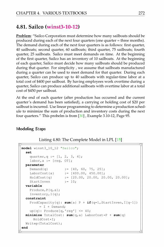
CHAPTER 4. VARIOUS TEXTBOOKS 272

4.81. Sailco (winst3-10-12)

Problem: “Sailco Corporation must determine how many sailboats should beproduced during each of the next four quarters (one quarter = three months).The demand during each of the next four quarters is as follows: first quarter,40 sailboats; second quarter, 60 sailboats; third quarter, 75 sailboats; fourthquarter, 25 sailboats. Sailco must meet demands on time. At the beginningof the first quarter, Sailco has an inventory of 10 sailboats. At the beginningof each quarter, Sailco must decide how many sailboats should be producedduring that quarter. For simplicity , we assume that sailboats manufacturedduring a quarter can be used to meet demand for that quarter. During eachquarter, Sailco can produce up to 40 sailboats with regular-time labor at atotal cost of $400 per sailboat. By having employees work overtime during aquarter, Sailco can produce additional sailboats with overtime labor at a totalcost of $450 per sailboat.

At the end of each quarter (after production has occurred and the currentquarter’s demand has been satisfied), a carrying or holding cost of $20 persailboat is incurred. Use linear programming to determine a production sched-ule to minimize the sum of production and inventory costs during the nextfour quarters.” This probelm is from [30] , Example 3.10-12, Page 95.

Modeling Steps

Listing 4.80: The Complete Model in LPL [15]� �model winst3_10_12 "Sailco";

setquarter,q := [1, 2, 3, 4];labor,a := [reg, OT];

parameterDemand{q} := [40, 60, 75, 25];LaborCost{a} := [400.00, 450.00];HoldCost{q} := [20.00, 20.00, 20.00, 20.00];StartInven := 10;

variableProduce,P{q,a};Inventory,I{q};

constraintProdCapacity{q}: sum{a} P + if(q=1,StartInven,I[q-1])

= I + Demand;up{q}: Produce[q,'reg'] <= 40;

minimize TotalCost: sum{q,a} LaborCost*P + sum{q}HoldCost*I;

Writep(TotalCost);end� �

273 CHAPTER 4. VARIOUS TEXTBOOKS

4.82. Farmer Jones (winstP3-1-1)

Problem: “Farmer Jones must detertnme how many acres of corn and wheatto plant this year. An acre of wheat yields bushels of wheat and requires 10hours of labor per week. An acre of corn yields 10 bushels of com and requires4 hours of labor per week. All wheat can be sold at $4 a bushel, and all corncan be sold at $3 a bushel. Seven acres of land and 40 hours per week of laborare available. Government regu-lations require that at least 30 bushels of cornbe produced during the current year. Let x1 = number of acres of corn planted,and x2 = number of acres of wheat planted. Using these decision variables,formulate an LP whose solution will tell Farmer Jones how to maximize thetotal revenue from wheat and corn.” This probelm is from [30] , Problem 3.1-1,Page 52.

Modeling Steps

Listing 4.81: The Complete Model in LPL [15]� �model winstP3_1_1 "Farmer Jones";

set grain := [Corn, Wheat];parameterYieldBushel{grain} := [10, 25]; -- bushels/acreReqLabor{grain} := [4, 10]; -- hours/acres/weekPrice{grain} := [3, 4]; -- $/bushelLandAvail := 7; -- acresLaborAvail := 40; -- hours/weekMinBushelsCorn := 30; -- bushels

variable PlantAcres {grain}; -- acresconstraintGovReq{grain|grain='Corn'}: YieldBushel*PlantAcres >=

MinBushelsCorn;Acres: sum{grain} PlantAcres <= LandAvail;HoursPerWeek: sum{grain} ReqLabor*PlantAcres <=

LaborAvail;maximize Revenue: sum{grain} Price*YieldBushel*

PlantAcres;Writep(Revenue);

end� �

CHAPTER 4. VARIOUS TEXTBOOKS 274

4.83. Farmer Jones (winstP3-1-1s)

Problem: “Farmer Jones must detertnme how many acres of corn and wheatto plant this year. An acre of wheat yields bushels of wheat and requires 10hours of labor per week. An acre of corn yields 10 bushels of com and requires4 hours of labor per week. All wheat can be sold at $4 a bushel, and all corncan be sold at $3 a bushel. Seven acres of land and 40 hours per week of laborare available. Government regu-lations require that at least 30 bushels of cornbe produced during the current year. Let x1 = number of acres of corn planted,and x2 = number of acres of wheat planted. Using these decision variables,formulate an LP whose solution will tell Farmer Jones how to maximize thetotal revenue from wheat and corn.” This probelm is from [30] , Problem 3.1-1,Page 52.

Modeling Steps

Listing 4.82: The Complete Model in LPL [15]� �model winstP3_1_1s "Farmer Jones";

variable Corn; Wheat; --acresconstraintAcres: Corn + Wheat <= 7;HoursPerWeek: 4*Corn + 10*Wheat <= 40;GovReq: 10*Corn >= 30;

maximize Revenue: 3*10*Corn + 4*25*Wheat;Writep(Revenue);

end� �

275 CHAPTER 4. VARIOUS TEXTBOOKS

4.84. Truck Corporation (winstP3-1-4)

Problem: “Truckco manufactures two types of trucks: 1 and 2. Each truckmust go through the painting shop and assembly shop. If the painting shopwere completely devoted to painting type 1 trucks, 800 per day could bepainted, whereas if the painting shop were completely devoted to paintingtype 2 trucks, 700 per day could be painted. If the assembly shop were com-pletely devoted to assembling truck 1 engines, 1500 per day could be assem-bled, and if the assembly shop were completely devoted to assembling truck2 engines, 1200 per day could be assembled. Each type 1 truck contributes$300 to profit; each type 2 truck contributes $500. Formulate an LP that willmaximize Truckco’s profit.” This probelm is from [30] , Problem 3.1-4, Page52.

Modeling Steps

Listing 4.83: The Complete Model in LPL [15]� �model winstP3_1_4 "Truck Corporation";

settruck := [1, 2];shop := [Painting, Assembly];

parameterProfit{truck} := [300, 500];CapPerDay{shop, truck} := [ 800, 700, 1500, 1200];

variable Produce{truck};constraint ProdCapacity{shop}: sum{truck} 1/CapPerDay*

Produce <= 1;maximize TotalProfit: sum{truck} Profit*Produce ;Writep(TotalProfit);

end� �

CHAPTER 4. VARIOUS TEXTBOOKS 276

4.85. Product-Mix (Truck Co) (winstP3-1-4s)

Problem: “Truckco manufactures two types of trucks: 1 and 2. Each truckmust go through the painting shop and assembly shop. If the painting shopwere completely devoted to painting type 1 trucks, 800 per day could bepainted, whereas if the painting shop were completely devoted to paintingtype 2 trucks, 700 per day could be painted. If the assembly shop were com-pletely devoted to assembling truck 1 engines, 1500 per day could be assem-bled, and if the assembly shop were completely devoted to assembling truck2 engines, 1200 per day could be assembled. Each type 1 truck contributes$300 to profit; each type 2 truck contributes $500. Formulate an LP that willmaximize Truckco’s profit.” This probelm is from [30] , Problem 3.1-4, Page52.

Modeling Steps

Listing 4.84: The Complete Model in LPL [15]� �model winstP3_1_4s "Product-Mix (Truck Co)";

variable Truck1; Truck2;constraintPainting: 1/800*Truck1 + 1/700*Truck2 <= 1;Body: 1/1500*Truck1 + 1/1200*Truck2 <= 1;

maximize Profit: 300*Truck1 + 500*Truck2;Writep(Profit);

end� �

277 CHAPTER 4. VARIOUS TEXTBOOKS

4.86. Leary Chemical (winstP3-2-3)

Problem: “Leary Chemical manufactures three chemicals: A, B, and C. Thesechemicals are produced via two production processes: l and 2. Running pro-cess for an hour costs S4 and yields 3 units of A, 1 of B, and 1 of C. Runningprocess 2 for an hour costs S1 and produces 1 unit of A and 1 of B. To meetcustomer demands, at least 10 units of A, 5 of B, and 3 of C must be produceddaily. Graphically determine a daily production plan that minimizes the costof meeting Leary Chemical’s daily demands.” This probelm is from [30] ,Problem 3.2-3, Page 60.

Modeling Steps

Listing 4.85: The Complete Model in LPL [15]� �model winstP3_2_3 "Leary Chemical";

setprocess := [P1, P2];chemical := [A, B, C];

parameterProcessCost{process} := [4.00, 1.00];ChemYield{chemical, process} := -- Units/hour

[3, 1, 1, 1, 1, 0];DailyDemand{chemical} := [10, 5, 3]; -- Units

variable RunHours{process}; -- hoursconstraintMeetDemand{chemical}: sum{process} ChemYield*RunHours

>= DailyDemand;minimize TotalCost: sum{process} ProcessCost*RunHours;Writep(TotalCost);

end� �

CHAPTER 4. VARIOUS TEXTBOOKS 278

4.87. Chemical Product Processes (winstP3-2-3s)

Problem: “Leary Chemical manufactures three chemicals: A, B, and C. Thesechemicals are produced via two production processes: l and 2. Running pro-cess for an hour costs S4 and yields 3 units of A, 1 of B, and 1 of C. Runningprocess 2 for an hour costs S1 and produces 1 unit of A and 1 of B. To meetcustomer demands, at least 10 units of A, 5 of B, and 3 of C must be produceddaily. Graphically determine a daily production plan that minimizes the costof meeting Leary Chemical’s daily demands.” This probelm is from [30] ,Problem 3.2-3, Page 60.

Modeling Steps

Listing 4.86: The Complete Model in LPL [15]� �model winstP3_2_3s "Chemical Product Processes";

variable Process1; Process2;constraintChemicalA: 3*Process1 + Process2 >= 10;ChemicalB: Process1 + Process2 >= 5;ChemicalC: Process1 >= 3;

minimize Cost: 4*Process1 + 1*Process2;Writep(Cost);

end� �

279 CHAPTER 4. VARIOUS TEXTBOOKS

4.88. Furniture Corporation (winstP3-2-5)

Problem: “Furnco manufactures desks and chairs. Each desk uses 4 units ofwood, and each chair uses 3. A desk contributes $40 to profit, and a chaircontributes $25. Marketing restntions require that the number of chairs pro-duced be at least twice the number of desks produced. If 20 units of woodare available, formulate an LP to maximize Furnco’s profit. Then graphicallysolve the LP.” This probelm is from [30] , Problem 3.2-5, Page 60.

Modeling Steps

Listing 4.87: The Complete Model in LPL [15]� �model winstP3_2_5 "Furniture Corporation";

set furniture := [Desks, Chairs];parameterProfit{furniture} := [40, 25];WoodUse{furniture} := [4, 3];WoodAvail := 20;

variable Produce{furniture};constraintWoodLimit: sum{furniture} WoodUse*Produce <=

WoodAvail;Marketing: 2*Produce['Chairs'] >= Produce['Desks'];

maximize TotalProfit: sum{furniture} Profit*Produce ;Writep(TotalProfit);

end� �

CHAPTER 4. VARIOUS TEXTBOOKS 280

4.89. Product-Mix (Furniture Corporation)(winstP3-2-5s)

Problem: “Furnco manufactures desks and chairs. Each desk uses 4 units ofwood, and each chair uses 3. A desk contributes $40 to profit, and a chaircontributes $25. Marketing restntions require that the number of chairs pro-duced be at least twice the number of desks produced. If 20 units of woodare available, formulate an LP to maximize Furnco’s profit. Then graphicallysolve the LP.” This probelm is from [30] , Problem 3.2-5, Page 60.

Modeling Steps

Listing 4.88: The Complete Model in LPL [15]� �model winstP3_2_5s "Product-Mix (Furniture Corporation)";

variable Desks; Chairs;constraintWoodAvail: 4*Desks + 3*Chairs <= 20;Marketing: 2*Chairs >= Desks;

maximize Profit: 40*Desks + 25*Chairs;Writep(Profit);

end� �

281 CHAPTER 4. VARIOUS TEXTBOOKS

4.90. Money Manager (winstP3-3-10s)

Problem: “Money manager Boris Milkem deals with French cur-rency (thefranc) and American currency (the dollar). At 12 midnight, he can buy francsby paying .25 dollars per franc and dollars by paying three francs per dol-lar. Let xi = num-ber of dollars bought (by paying francs) and x2 = numberof francs bought (by paying dollars). Assume that both types of transactionstake place simultaneously, and the only constraint is that at 12:01 A.M., Borismust have a nonnegative number of francs and dollars.

a Formulate an LP that enables Boris to maximize the number of dollars hehas after all transactions are completed.

b Graphically solve the LP and comment on the answer.”

This probelm is from [30] , Problem 3.3-10, Page 66.

Modeling Steps

Listing 4.89: The Complete Model in LPL [15]� �model winstP3_3_10s "Money Manager";

variable Dollars; Francs;constraintMinDollars: Dollars + 0.25*Francs >= 0;MinFrancs: 3*Dollars + Francs >= 0;

maximize TotalDollars: Dollars - 0.25*Francs;Writep(TotalDollars,Dollars,Francs);Write('The model is infeasible\n');

end� �

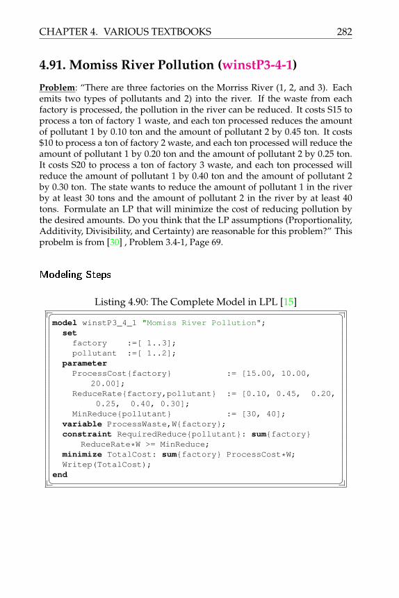
CHAPTER 4. VARIOUS TEXTBOOKS 282

4.91. Momiss River Pollution (winstP3-4-1)

Problem: “There are three factories on the Morriss River (1, 2, and 3). Eachemits two types of pollutants and 2) into the river. If the waste from eachfactory is processed, the pollution in the river can be reduced. It costs S15 toprocess a ton of factory 1 waste, and each ton processed reduces the amountof pollutant 1 by 0.10 ton and the amount of pollutant 2 by 0.45 ton. It costs$10 to process a ton of factory 2 waste, and each ton processed will reduce theamount of pollutant 1 by 0.20 ton and the amount of pollutant 2 by 0.25 ton.It costs S20 to process a ton of factory 3 waste, and each ton processed willreduce the amount of pollutant 1 by 0.40 ton and the amount of pollutant 2by 0.30 ton. The state wants to reduce the amount of pollutant 1 in the riverby at least 30 tons and the amount of pollutant 2 in the river by at least 40tons. Formulate an LP that will minimize the cost of reducing pollution bythe desired amounts. Do you think that the LP assumptions (Proportionality,Additivity, Divisibility, and Certainty) are reasonable for this problem?” Thisprobelm is from [30] , Problem 3.4-1, Page 69.

Modeling Steps

Listing 4.90: The Complete Model in LPL [15]� �model winstP3_4_1 "Momiss River Pollution";

setfactory :=[ 1..3];pollutant :=[ 1..2];

parameterProcessCost{factory} := [15.00, 10.00,

20.00];ReduceRate{factory,pollutant} := [0.10, 0.45, 0.20,

0.25, 0.40, 0.30];MinReduce{pollutant} := [30, 40];

variable ProcessWaste,W{factory};constraint RequiredReduce{pollutant}: sum{factory}

ReduceRate*W >= MinReduce;minimize TotalCost: sum{factory} ProcessCost*W;Writep(TotalCost);

end� �

283 CHAPTER 4. VARIOUS TEXTBOOKS

4.92. US Lab (winstP3-4-2)

Problem: “U.S. Labs manufactures mechanical heart valves from the heartvalves of pigs. Different heart operations require valves of different sizes.U.S. Labs purchases pig valves from three different suppliers. The cost andsize mix of the valves purchased from each supplier are given in Table 4.22.Each month, U.S. Labs places one order with each supplier. At least 590Jarge,300 medium, and 300 small valves must be purchased each month. Becauseof limited availability of pig valves, at most 500 valves per month can be pur-chased from each supplier. Formulate an LP that can be used to minimizethe cost of acquiring the needed valves.” This problem is from [30] , Problem3.4-2, Page 69.

Cost Percent Percent PercentPer Value Large Medium Small

Supplier 1 $5 40 40 20Supplier 2 $4 30 35 35Supplier 3 $3 20 20 60

Table 4.4:

Modeling Steps

Listing 4.91: The Complete Model in LPL [15]� �model winstP3_4_2 "US Lab";

set supplier :=[ 1..3];valve := [Large, Medium, Small];

parameter CostValve{supplier} := [5.00, 4.00, 3.00];PurchaseMix{supplier, valve} := [0.40, 0.40, 0.20,

0.30, 0.35, 0.35, 0.20, 0.20, 0.60];--MaxPurchase{supplier} := [500, 500, 500]; --not

feasibe with this dataMaxPurchase{supplier} := [600, 600, 600];ReqPurchase{valve} := [500, 300, 300];

variable Purchase,P{supplier} [0..MaxPurchase];constraintRequiredPurchase{valve}: sum{supplier} PurchaseMix*P

>= ReqPurchase;minimize TotalCost: sum{supplier,valve} CostValve*P;Writep(TotalCost);

end� �

CHAPTER 4. VARIOUS TEXTBOOKS 284

4.93. Diet Problem (winstP3-4-3)

Problem: “Peg and Al Fundy have a limited food budget, so eg is trying tofeed the family as cheaply as possible. However, she still wants to make sureher family members meet their daily nutritional requirements. Peg can buytwo foods. Food 1 sells for $7 per pound, and each pound contains 3 units ofvitamin A and 1 unit of vitamin C. Food 2 sells for $1 per pound, and eachpound contains 1 unit of each vitamin. Each day, the family needs at least 12units of vitamin A and 6 units of vitamin C.

a) Verify that Peg should purchase 12 units of food 2 each day and thus over-satisfy the vitamin C requirement by 6 units.

b) Al has put his foot down and demanded that Peg fulfill the family’s dailynutritional requirement exactly by obtaining precisely 12 units of vitamin Aand 6 units of vitamin C. The optimal solution to the new problem will in-volve ingesting less vitamin C, but it will be more expensive. Why?”This problem is from [30] , Problem 3.4-3, Page 69.

Modeling Steps

Listing 4.92: The Complete Model in LPL [15]� �model winstP3_4_3 "Diet Problem";

setf :=[ 1..2] "Food";v := [A, C] "Vitamin";

parameterFoodCost{f} := [7, 1];AmountVitamin{f, v} := [3, 1, 1, 1];MinDailyReq{v} := [12, 6];

variable Purchase{f};constraintRequirement{v}: sum{f} AmountVitamin*Purchase >=

MinDailyReq;minimize TotalCost: sum{f} FoodCost*Purchase;Writep(TotalCost);

end� �

285 CHAPTER 4. VARIOUS TEXTBOOKS

4.94. Gold Mining (winstP3-4-4)

Problem: “Goldilocks needs to find at least 12 lb of gold and at least 18 lb ofsilver to pay the monthly rent. There are two mines in which Goldilocks canfind gold and silver. Each day that Goldilocks spends in mine 1, she finds2 lb of gold and 2 lb of silver. Each day that Goldilocks spends in mine 2,she finds 1 lb of gold and 3 lb of silver. Formulate an LP to help Goldilocksmeet her requirements while spending as little time as possible in the mines.Graphically solve the LP.” This probelm is from [30] , Problem 3.4-4, Page 69.

Modeling Steps

Listing 4.93: The Complete Model in LPL [15]� �model winstP3_4_4 "Gold Mining";

setmine :=[ 1..2];metals := [gold, silver];

parameterDiscover{mine, metals} := [2, 2, 1, 3];MetalReq{metals} := [12, 18];

variable DaysSpent{mine};constraint Requirement{metals}: sum{mine} Discover*

DaysSpent >= MetalReq;minimize TotalDays: sum{mine} DaysSpent;Writep(TotalDays);

end� �

CHAPTER 4. VARIOUS TEXTBOOKS 286

4.95. Capital Budget (winstP3-6-2)

Problem: “Two investments with varying cash flows (in thousands of dol-lars) are available, as shown in Table 4.22. At time 0, $10,000 is available forinvestment, and at time 1, $7000 is available. Assuming that r = 0.10, set upan LP whose so-lution maximizes the NPV obtained from these investments.Graphically find the optimal solution to the LP. (Assume that any fraction ofan investment may be purchased).” This probelm is from [30] , Problem 3.6-2,Page 76.

Cash Flow (in thousands) at Time0 1 2 3

Investment 1 -$6 -$5 $7 $9Investment 2 -$8 -$3 $9 $7

Table 4.5:

Modeling Steps

Listing 4.94: The Complete Model in LPL [15]� �model winstP3_6_2 "Capital Budget";

settime := [0..3];invest := [1..2];

parameterCashAvail{time} := [10, 7, 0, 0];CashFlow{invest,time} := [-6 -5 7 9 -8 -3 9 7];InterestRate := 0.1;RateMult := 1.0 + InterestRate;NPV{invest} := sum{time} CashFlow/RateMult^time;

variable MakeInvest{invest} [0..1];constraint InvestLimit{time}: sum{invest} - CashFlow*

MakeInvest <= CashAvail;maximize TotalProfit: sum{invest} NPV*MakeInvest ;Writep(TotalProfit,MakeInvest);

end� �

287 CHAPTER 4. VARIOUS TEXTBOOKS

4.96. Blending Candy (winstP3-8-1)

Problem: “You have decided to enter the candy business. You are consideringproducing two types of candies: Slugger Candy and Easy Out Candy, both ofwhich consist solely of sugar, nuts, and chocolate. At present, you have instock 100 oz of sugar, 20 oz of nuts, and 30 oz of chocolate. The mixtureused to make Easy Out Candy must contain at least 20mixture used to makeSlugger Candy must contain at least 10can be sold for 250, and each ounceof Slugger Candy for 200. Formulate an LP that will enable you to maximizeyour revenue from candy sales.” This probelm is from [30] , Problem 3.8-1,Page 87.

Modeling Steps

Listing 4.95: The Complete Model in LPL [15]� �model winstP3_8_1 "Blending Candy";

setcandy := [Slugger, EasyOut];ingred := [Sugar, Nuts, Chocolate];

parameterPrice{candy} := [0.20, 0.25];AvailIngred{ingred} := [100, 20, 30];MinPercent{candy,ingred}:=[0, 0.1, 0.1, 0, 0.2, 0];

variable SweetMix{candy,ingred};constraintMinIngred{candy,ingred|MinPercent>0}: SweetMix >=

MinPercent*(sum{ingred} SweetMix);MaxIngread{ingred}: sum{candy} SweetMix <=

AvailIngred;maximize TotalProfit: sum{candy,ingred} Price*SweetMix;Writep(TotalProfit);

end� �

CHAPTER 4. VARIOUS TEXTBOOKS 288

4.97. Blending Oranges (winstP3-8-2)

Problem: “O.J. Juice Company sells bags of oranges and cartons of orangejuice. O.J. grades oranges on a scale of 1 (poor) to 10 (excellent). At present,Q.J. has on hand 100,000 lb of grade 9 oranges and 120,000 lb of grade 6 or-anges. The average quality of oranges sold in bags must be at least 7, and theaverage quality of the oranges used to produce orange juice must be at least8. Each pound of oranges that is used for juice yields a revenue of $1.50 andincurs a variable cost (consisting of labor costs, variable overhead costs, in-ventory costs, and so on) of $1.05. Each pound of oranges sold in bags yieldsa revenue of 50 cents and incurs a variable cost of 200. Formulate an LP tohelp O.J. maximize profit.” This probelm is from [30] , Problem 3.8-2, Page 87.

Modeling Steps

Listing 4.96: The Complete Model in LPL [15]� �model winstP3_8_2 "Blending Oranges";

setgrade := [g6, g9];product := [Juice, Bags];

parameterGradeValue{grade} := [6, 9];OrangesOnHand{grade} := [100000, 120000];MinAvgQuality{product} := [8, 7];Revenue{product} := [1.50, 0.50];VarCost{product} := [1.05, 0.20];Profit{product} := Revenue - VarCost;

variable Produce{grade,product};constraintLimitOranges{grade}: sum{product} Produce <=

OrangesOnHand;ReqQuality{product}: sum{grade} GradeValue*Produce >=

MinAvgQuality*(sum{grade} Produce);maximize TotalProfit: sum{grade,product} Profit*Produce

;Writep(TotalProfit);

end� �

289 CHAPTER 4. VARIOUS TEXTBOOKS

4.98. Blending Portfolio (winstP3-8-3)

Problem: “A bank is attempting to determine where its assets should be in-vested during the current year. At present, $500,000 is available for invest-ment in bonds, home loans, auto loans, and personal loans. The annual rateof return on each type of investment is known to be: bonds, 10auto loans,13bank’s portfolio is not too risky, the bank’s investment man- ager has placedthe following three restrictions on the bank’s portfolio:

a) The amount invested in personal loans cannot ex- ceed the amount investedin bonds.

b) The amount invested in home loans cannot exceed the amount invested inauto loans.

c) No more than 25be in personal loans.

The bank’s objective is to maximize the annual return on its investment port-folio. Formulate an LP that will enable the bank to meet this goal.” Thisproblem is from [30] , Problem 3.8-3, Page 87.

Modeling Steps

Listing 4.97: The Complete Model in LPL [15]� �model winstP3_8_3 "Blending Portfolio";

set portfolio := [Bonds, Home, Auto, Personal];parameterCashAvail := 500000;ReturnRate{portfolio} := [0.10, 0.16, 0.13, 0.20];PercentPersonal := 0.25;

variable Invest{portfolio};constraintMaxInvestment: sum{portfolio} Invest <= CashAvail;PersonalLomit: Invest['Personal'] <= Invest['Bonds'];HomeLimit: Invest['Home'] <= Invest['Auto'];MaxPersonal: Invest['Personal'] <= PercentPersonal*(

sum{portfolio} Invest);maximize TotalProfit: sum{portfolio} ReturnRate*Invest;Writep(TotalProfit);

end� �

CHAPTER 4. VARIOUS TEXTBOOKS 290

4.99. Blending Investments (winstP3-8-4)

Problem: “Young MBA Erica Cudahy may invest up to $1000. She can investher money in stocks and loans. Each dollar invested in stocks yields 10 centsprofit, and each dollar invested in a loan yields 15 cents profit. At least 30%of all money invested must be in stocks, and at least $400 must be in loans.Formulate any that can be used to maximize total profit earned from Erica’sinvestment. Then graphically solve the LP.” This probelm is from [30] , Prob-lem 3.8-4, Page 87.

Modeling Steps

Listing 4.98: The Complete Model in LPL [15]� �model winstP3_8_4 "Blending Investments";

set invest := [Stocks, Loans];parameterMaxAmountAvail := 1000;MinStockPercent := 0.30;MinLoanAmount := 400.00;ProfitPerDollar{invest} := [0.10, 0.15];

variable Amount{invest};constraintTotalInvestment: sum{invest} Amount<=MaxAmountAvail;MinStocks: Amount['Stocks'] >= MinStockPercent*(sum{

invest} Amount);MinLoans: Amount['Loans'] >= MinLoanAmount;

maximize TotalProfit: sum{invest} ProfitPerDollar*Amount;

Writep(TotalProfit);end� �

291 CHAPTER 4. VARIOUS TEXTBOOKS

4.100. Blending Oils (winstP3-8-5)

Problem: “Chandler Oil Company has 5000 barrels of oil 1 and 3.8 BlendingProblems 87 10,000 barrels of oil 2. The company sells two products: gasolineand heating oil. Both products are produced by combining oil 1 and oil 2. Thequality level of each oil is as follows: oil 1, 10; oil 2, 5. Gasoline must havean average quality level of at least 8 and heating oil, at least 6. Demand foreach product must be created by advertising. Each dollar spent advertisinggasoline creates 5 barrels of demand and each spent on heating oil creates10 barrels of demand. Gaso- line is sold for $25 per barrel, heating oil for$20. Formulate an LP to help Chandler maximize profit. Assume that no oilof either type can be purchased.” This probelm is from [30] , Problem 3.8-5,Page 87.

Modeling Steps

Listing 4.99: The Complete Model in LPL [15]� �model winstP3_8_5 "Blending Oils";

setoiltype,o := [Oil1, Oil2];product,p := [Gasoline, HeatingOil];

parameterBarrelsAvail{o} := [5000, 10000];QualityLevel{o} := [10, 5];QualityReq{p} := [8, 6];Price{p} := [25.00, 20.00];DemandPerAdDollar{p} := [5, 10];

variableBlend,B{p,o};AdDollars,A{p};

constraintMinAvgQuality{p}: sum{o} QualityLevel*B >= QualityReq

*(sum{o} B);MaxOilAvail{o}: sum{p} B <= BarrelsAvail;AdSpending{p}: sum{o} B = DemandPerAdDollar*A;

maximize TotalProfit: sum{p,o} Price*B - sum{p} A;Writep(TotalProfit);

end� �

CHAPTER 4. VARIOUS TEXTBOOKS 292

4.101. Blending Oils (winstP3-8-5b)

Problem: “Chandler Oil Company has 5000 barrels of oil 1 and 3.8 BlendingProblems 87 10,000 barrels of oil 2. The company sells two products: gasolineand heating oil. Both products are produced by combining oil 1 and oil 2. Thequality level of each oil is as follows: oil 1, 10; oil 2, 5. Gasoline must havean average quality level of at least 8 and heating oil, at least 6. Demand foreach product must be created by advertising. Each dollar spent advertisinggasoline creates 5 barrels of demand and each spent on heating oil creates10 barrels of demand. Gaso- line is sold for $25 per barrel, heating oil for$20. Formulate an LP to help Chandler maximize profit. Assume that no oilof either type can be purchased.” This probelm is from [30] , Problem 3.8-5,Page 87.

Modeling Steps

Listing 4.100: The Complete Model in LPL [15]� �model winstP3_8_5b "Blending Oils";

setoiltype,o := [Oil1, Oil2];product,p := [Gasoline, HeatingOil];

parameterBarrelsAvail{o} := [5000, 10000];QualityLevel{o} := [10, 5];QualityReq{p} := [8, 6];Price{p} := [25.00, 20.00];DemandPerAdDollar{p} := [5, 10];

variableBlend,B{p,o};Produce,P{p};AdDollars,A{p};

constraintBlendOil{p}: P = sum{o} B;MinAvgQuality{p}: sum{o} QualityLevel*B >= QualityReq

*P;MaxOilAvail{o}: sum{p} B <= BarrelsAvail;AdSpending{p}: P = DemandPerAdDollar*A;

maximize TotalProfit: sum{p} Price*P - sum{p} A;Writep(TotalProfit);

end� �

293 CHAPTER 4. VARIOUS TEXTBOOKS

4.102. Blending fertilizer (winstP3-8-6)

Problem: “Bullco blends silicon and nitrogen to produce two types of fertiliz-ers. Fertilizer 1 must be at least 40sells for $70/lb. Fertilizer 2 must be at least70sells for $40/lb. Bullco can purchase up to 80 lb of nitrogen at $15/1b andup to 100 lb of silicon at $10/1b. Assuming that all fertilizer produced can besold, formulate an LP to help Bullco maximize profits. ” This probelm is from[30] , Problem 3.8-6, Page 87.

Modeling Steps

Listing 4.101: The Complete Model in LPL [15]� �model winstP3_8_6 "Blending fertilizer";

setfertilizer := [f1, f2];component := [Silicon, Nitrogen];

parameterProfit{fertilizer} := [70.00, 40.00];Percent{fertilizer, component} := [0, 0.40, 0.70, 0];Cost{component} := [15.00, 10.00];MaxPurchase{component} := [80, 100];

variable Blend{fertilizer,component};constraintRequire{fertilizer,component|Percent>0}: Blend >=

Percent*(sum{component} Blend);MaxComponent{component}: sum{fertilizer} Blend <=

MaxPurchase;maximize TotalProfit: sum{fertilizer,component} (Profit

*Blend - Cost*Blend);Writep(TotalProfit,Blend);

end� �

CHAPTER 4. VARIOUS TEXTBOOKS 294

4.103. Blending chemicals (winstP3-8-7)

Problem: “Eli Daisy uses chemicals 1 and 2 to produce two drugs. Drug 1must be at least 70at least 60at $6 per oz; up to 30 oz of drug 2 can be sold at$5 per oz. Up to 45 oz of chemical 1 can be purchased at $6 per oz, and up to40 oz of chemical 2 can be purchased at $4 per oz. Formulate an LP that canbe used to maximize Daisy’s profits. ” This probelm is from [30] , Problem3.8-7, Page 87.

Modeling Steps

Listing 4.102: The Complete Model in LPL [15]� �model winstP3_8_7 "Blending chemicals";

setchemical,c := [c1, c2];drug ,d := [d1, d2];

parameterMinChemPercent{d,c} := [0.70, 0 0, 0.60];MaxDemand{d} := [40, 30];Price{d} := [6.00, 5.00];MaxChemAvail{c} := [45, 40];Cost{c} := [6.00, 4.00];

variable MixChem{c,d};constraintRequirement{d,c|MinChemPercent>0}: MixChem >=

MinChemPercent*(sum{c} MixChem);LimitDemand{d}: sum{c} MixChem <= MaxDemand;LimitChemical{c}: sum{d} MixChem <= MaxChemAvail;

maximize TotalProfit: sum{d} Price*(sum{c} MixChem) -sum{c} Cost*(sum{d} MixChem);

Writep(TotalProfit);end� �

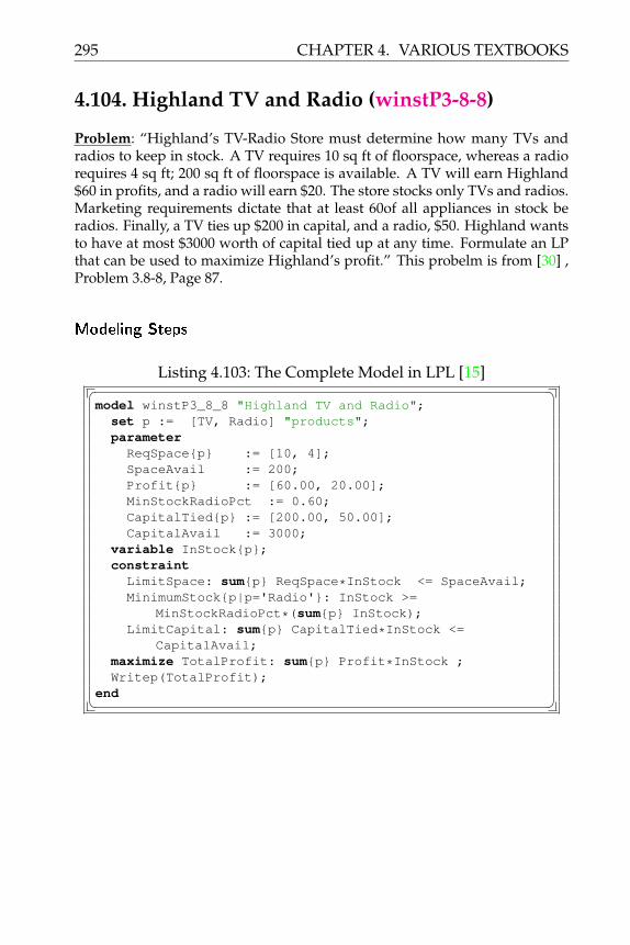
295 CHAPTER 4. VARIOUS TEXTBOOKS

4.104. Highland TV and Radio (winstP3-8-8)

Problem: “Highland’s TV-Radio Store must determine how many TVs andradios to keep in stock. A TV requires 10 sq ft of floorspace, whereas a radiorequires 4 sq ft; 200 sq ft of floorspace is available. A TV will earn Highland$60 in profits, and a radio will earn $20. The store stocks only TVs and radios.Marketing requirements dictate that at least 60of all appliances in stock beradios. Finally, a TV ties up $200 in capital, and a radio, $50. Highland wantsto have at most $3000 worth of capital tied up at any time. Formulate an LPthat can be used to maximize Highland’s profit.” This probelm is from [30] ,Problem 3.8-8, Page 87.

Modeling Steps

Listing 4.103: The Complete Model in LPL [15]� �model winstP3_8_8 "Highland TV and Radio";

set p := [TV, Radio] "products";parameterReqSpace{p} := [10, 4];SpaceAvail := 200;Profit{p} := [60.00, 20.00];MinStockRadioPct := 0.60;CapitalTied{p} := [200.00, 50.00];CapitalAvail := 3000;

variable InStock{p};constraintLimitSpace: sum{p} ReqSpace*InStock <= SpaceAvail;MinimumStock{p|p='Radio'}: InStock >=

MinStockRadioPct*(sum{p} InStock);LimitCapital: sum{p} CapitalTied*InStock <=

CapitalAvail;maximize TotalProfit: sum{p} Profit*InStock ;Writep(TotalProfit);

end� �

CHAPTER 4. VARIOUS TEXTBOOKS 296

4.105. Production Process (Sunco Oil) (winstP3-9-1)

Problem: “Sunco Oil has three different processes that can be used to manu-facture various types of gasoline. Each process in-volves blending oils in thecompany’s catalytic cracker. Run-ning process 1 for an hour costs $5 and re-quires 2 barrels of crude oil 1 and 3 barrels of crude oil 2. The output fromrunning process 1 for an hour is 2 barrels of gas 1 and 1 barrel of gas 2. Run-ning process 2 for an hour costs $4 and requires 1 barrel of crude 1 and 3barrels of crude 2. The output from running process 2 for an hour is 3 bar-rels of gas 2. Running process 3 for all hour costs $1 and requires 2 barrelsof crude 2 and 3 barrels of gas 2. The output from running process 3 for anhour is 2 barrels of gas 3. Each week , 200 barrels of crude 1, at $2/barrel,and 300 barrels of crude 2, at $3/bar-rel, may be purchased. All gas producedcan be sold at the following per-barrel prices: gas 1, $9; gas 2, $10; gas 3, $24.Formulate an LP whose solution will maximize revenues less costs. Assumethat only 100 hours of time on the catalytic cracker are available each week.”This probelm is from [30] , Problem 3.9-1, Page 93.

Modeling Steps

Listing 4.104: The Complete Model in LPL [15]� �model winstP3_9_1 "Production Process (Sunco Oil)";

set process := [1..3];crude := [1..2]; gas := [1..3];

parameter RunCost{process} := [5, 4, 1];CrudeReq{process,crude}:= [2, 3, 1, 3, 0, 2];GasReq{process, gas} := [0 0 0 0 0 0 0 3 0];OutputGas{process,gas} := [2 1 0 0 3 0 0 0 2];MaxPurchase{crude} := [200, 300];CrudeCost{crude} := [2.00, 3.00];GasPrice{gas} := [9.00, 10.00, 24.00];MaxCrackerHours := 100;

variableSalesGas{gas}; RunProcess{process};PurchaseCrude{crude};

constraintCrackerLimit: sum{process} RunProcess <=

MaxCrackerHours;CrudeBalance{crude}: PurchaseCrude = sum{process}

CrudeReq*RunProcess;PurchaseLimit{crude}: PurchaseCrude <= MaxPurchase;GasBalance{gas}: sum{process} OutputGas*RunProcess

= sum{process} GasReq*RunProcess + SalesGas;maximize TotalProfit: sum{gas} GasPrice*SalesGas- sum{process} RunCost*RunProcess

297 CHAPTER 4. VARIOUS TEXTBOOKS

- sum{crude} CrudeCost*PurchaseCrude;Writep(TotalProfit);

end� �

CHAPTER 4. VARIOUS TEXTBOOKS 298

4.106. Production Process (winstP3-9-2)

Problem: “Furnco manufactures tables and chairs. A table requires 40 boardft of wood, and a chair requires 30 board ft of wood. Wood may be purchasedat a cost of $1 per board ft, and 40,000 board ft of wood are available for pur-chase. It takes 2 hours of skilled labor to manufacture an unfinished table oran unfinished chair. Three more hours of skilled labor will turn an unfinishedtable into a finished table, and 2 more hours of skilled labor will turn an un-finished chair into a finished chair. A total of 6000 hours of skilled labor areavailable (and have already been paid for). All furniture produced can be soldat the following unit prices: unfinished table, $70; finished table, $140; unfin-ished chair, $60; finished chair, $110. Formulate an LP that will maximize thecontribution to profit from manufacturing tables and chairs. ” This probelmis from [30] , Problem 3.9-2, Page 93.

Modeling Steps

Listing 4.105: The Complete Model in LPL [15]� �model winstP3_9_2 "Production Process";

setf := [Desks, Chairs] "furniture";s := [Unfinished, Finished] "status";

parameterWoodUse{f} := [40, 30];WoodCost := 1;WoodAvail := 40000;LaborNeeded{f,s} := [2, 5, 2, 4];HoursAvail := 6000;Price{f,s} := [70, 140, 60, 110];

variableProduce{f,s};WoodPurchase [0..WoodAvail];

constraintWoodLimit: sum{f, s} WoodUse*Produce <= WoodPurchase;LaborLimit: sum{f, s} LaborNeeded*Produce <=

HoursAvail;maximize TotalProfit: sum{f,s} Price*Produce

- WoodCost*WoodPurchase;Writep(TotalProfit);

end� �

299 CHAPTER 4. VARIOUS TEXTBOOKS

4.107. Production Process (Rylon Corp.)(winstP3-9-3)

Problem: “Rylon Corporation manufactures Brute and Chanelle perfumes.The raw material needed to manufacture each type of perfume can be pur-chased for $3 per pound. Processing 1 lb of raw material requires 1 hour oflaboratory time. Each pound of processed raw material yields 3 oz of Regu-lar Brute Perfume and 4 oz of Regular Chanelle Perfume. Regular Brute canbe sold for $7/oz and Regular Chanelle for $6/oz. Rylon also has the optionof further processing Regular Brute and Regular Chanelle to produce LuxuryBrute, sold at $18/oz, and Luxury Chanelle, sold at $14/oz. Each ounce ofRegular Brute processed further requires an additional 3 hours of laboratorytime and $4 processing cost and yields 1 oz of Luxury Brute. Each ounce ofRegular Chanelle processed further requires an additional 2 hours of labora-tory time and $4 processing cost and yields 1 oz of Luxury Chanelle. Eachyear, Rylon has 6000 hours of laboratory time available and can purchase upto 4000 lb of raw material. Formulate an LP that can be used to determine howRylon can maximize profits. Assume that the cost of the laboratory hours is afixed cost.

Suppose that in Example (3.9-11), 1 lb of raw material could be used to pro-duce either 3 oz of Brute or 4 oz of Chanelle. How would this change theformulation? ” This probelm is from [30] , Problem 3.9-3, Page 93.

Modeling Steps

Listing 4.106: The Complete Model in LPL [15]� �model winstP3_9_3 "Production Process (Rylon Corp.)";

setp := [Brute, Chanele] "perfumes";t := [Regular, Luxury] "types";

parameterRawMatCost := 3.00; --$/lbRawMatYield{p} := [3, 4]; --oz/lbLabTimeRaw := 1; --Hours/lbLabTimeLux{p} := [3, 2]; --Hours/ozPrice{p, t} := [7, 18,

6, 14]; --$/ozProcessCost{p} := [4, 4]; --$/ozLabTimeAvail := 6000;RawMatAvail := 4000;

variableSales{p, t}; --ozRawMatPurchased{p}; --lb

expression

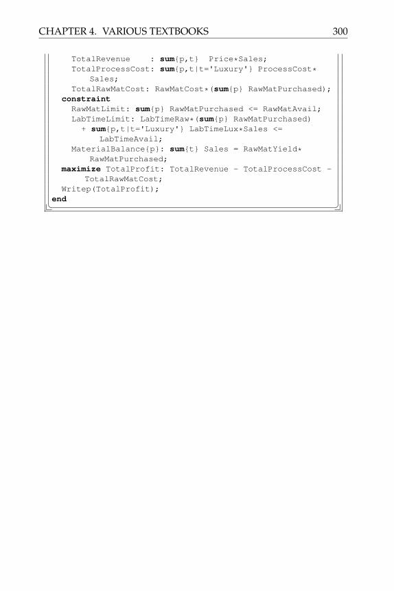
CHAPTER 4. VARIOUS TEXTBOOKS 300

TotalRevenue : sum{p,t} Price*Sales;TotalProcessCost: sum{p,t|t='Luxury'} ProcessCost*

Sales;TotalRawMatCost: RawMatCost*(sum{p} RawMatPurchased);

constraintRawMatLimit: sum{p} RawMatPurchased <= RawMatAvail;LabTimeLimit: LabTimeRaw*(sum{p} RawMatPurchased)

+ sum{p,t|t='Luxury'} LabTimeLux*Sales <=LabTimeAvail;

MaterialBalance{p}: sum{t} Sales = RawMatYield*RawMatPurchased;

maximize TotalProfit: TotalRevenue - TotalProcessCost -TotalRawMatCost;

Writep(TotalProfit);end� �

301 CHAPTER 4. VARIOUS TEXTBOOKS

4.108. Production Process (winstP3-9-5)

Problem: “A company produces A, B, and C and can sell these products inunlimited quantities at the following unit prices: A, $10; B, $56; C, $100. Pro-ducing a unit of A requires 1 hour of labor; a unit of B, 2 hours of labor plus2 units of A; and a unit of C, 3 hours of labor plus 1 unit of B. Any A that isused to produce B cannot be sold. Similarly, any B that is used to produce Ccannot be sold. A total of 40 hours of labor are available. Formulate an LPto maximize the company’s revenues. ” This probelm is from [30] , Problem3.9-5, Page 93.

Modeling Steps

Listing 4.107: The Complete Model in LPL [15]� �model winstP3_9_5 "Production Process";

set product,p,p1 := [A, B, C];parameterPrice{p} := [10, 56, 100];ProdHours{p} := [1, 2, 3];BillOfMat{p,p1} := /A B 2, B C 1/;HoursAvail := 40;

variableProduce{p};Sales{p};

constraintLimitProduction: sum{p} ProdHours*Produce <=

HoursAvail;ProdBalance{p1}: Produce = sum{p} BillOfMat*Produce +

Sales;maximize Revenues: sum{p} Price*Sales ;Writep(Revenues);

end� �

CHAPTER 4. VARIOUS TEXTBOOKS 302

4.109. Production Process (Daisy Drug)(winstP3-9-6)

Problem: “Daisy Drugs manufactures two drugs: 1 and 2. The dru2s are pro-duced by blending two chemicals: 1 and 2. By weigh-t, drug 1 must containat least 65contain at least 55drug 2 sells for $4/oz. Chemicals 1 and 2 can beproduced by one of two production processes. Running process 1 for an hourrequires 3 oz of raw material and 2 hours skilled labor and yields 3 oz of eachchemical. Running process 2 for an hour requires 2 oz of raw material and3 hours of skilled labor and yields 3 oz of chemical 1 and 1 oz of chemical 2.A total of 120 hours of skilled labor and 100 oz of raw material are available.Formulate an LP that can be used to maximize Daisy’s sales revenues. ” Thisprobelm is from [30] , Problem 3.9-6, Page 93.

Modeling Steps

Listing 4.108: The Complete Model in LPL [15]� �model winstP3_9_6 "Production Process (Daisy Drug)";

setdrug :=[ 1..2];chemical :=[ 1..2];process :=[ 1..2];

parameterPercentReq{drug, chemical} := [0.65, 0, 0, 0.55];Price{drug} := [6, 4];LaborUse{process} := [2, 3];RawMatUse{process} := [3, 2];ChemicalYield{process, chemical} := [3, 3, 3, 1];LaborAvail := 120;RawMatAvail := 100;

variableRunProcess,R{process};Blend,B{chemical,drug};

constraintLaborLimit: sum{process} LaborUse*R <= LaborAvail;RawMatLimit: sum{process} RawMatUse*R <= RawMatAvail;ChemBalance{chemical}: sum{process} ChemicalYield*R

>= sum{drug} B;RequireChem{drug,chemical|PercentReq>0}: B >=

PercentReq*(sum{chemical} B);maximize TotalRevenue: sum{chemical,drug} Price*B;Writep(TotalRevenue);

end� �

303 CHAPTER 4. VARIOUS TEXTBOOKS

4.110. Production Process (Lizzies Dairy)(winstP3-9-7)

Problem: “ Lizzie’s Dairy produces cream cheese and cottage cheese. Milkand cream are blended to produce these two products. Both high-fat andlow-fat milk can be used to pro- duce cream cheese and cottage cheese. High-fat milk is 60% fat; low-fit milk is 30% fat. The milk used to produce creamcheese must average at least 50% fat and that for cottage cheese, at least 35%fat. At least 40% (by weight) of the inputs to cream cheese and at least 20%(by weight) of the inputs to cottage cheese must be cream. Both cottage cheeseand cream cheese are produced by putting milk and cream through the cheesemachine. It costs 40c to process 1 lb of inputs into a pound of cream cheese. Itcosts 40 cents to produce 1 lb of cottage cheese, but every pound of input forcottage cheese yields 0.9 lb of cottage cheese and 0.1 lb of waste. Cream can beproduced by evaporating high-tat and low-fatmilk. It costs 40 cents to evap-orate I lb of high-fat milk. Each, pound of high-fat milk that is evaporatedyields 0.6 lb of cream. It costs 40 cents to evaporate 1 lb of low-fat milk. Eachpound of low-fat milk that is evaporated yields 0.3 lb of cream. Each day, upto 3000 lb of input may be sent through the cheese machine. Each day, at least1000 lb of cottage cheese and 1000 lb of cream cheese must be produced. Upto 1500 lb of cream cheese and 2000 lb of cottage cheese can be sold each day.Cottage cheese is sold for $1.20/1b and cream cheese for $1.50/1b. High-fatmilk is purchased for 80 cents/lb and low-fat milk for 40 cents/lb. The evap-orator can process at most 2000 lb of milk daily. Formulate an LP that can heused to maximize Lizzie ’s daily profit.” This probelm is from [30] , Problem3.9-7, Page 93.

Modeling Steps

Listing 4.109: The Complete Model in LPL [15]� �model winstP3_9_7 "Production Process (Lizzies Dairy)";

setcheese := [CreamCheese, CottageCheese];milk := [HiFatMilk, LowFatMilk];

parameterFatContent{milk} := [0.60, 0.30];MinFatPct{cheese} := [0.50, 0.35];MinCreamPct{cheese} := [0.40, 0.20];EvapYield{milk} := [0.6, 0.3];EvapCost{milk} := [0.40, 0.40];EvapCapacity := 2000;ProcessYield{cheese} := [1.0, 0.9];ProcessCost{cheese} := [0.40, 0.40];ProcessCapacity := 3000;

CHAPTER 4. VARIOUS TEXTBOOKS 304

MinProduce{cheese} := [1000, 1000];MaxProduce{cheese} := [1500, 2000];MilkCost{milk} := [0.80, 0.40];CheesePrice{cheese} := [1.50, 1.20];

variableProduceCheese,P{cheese} [MinProduce..MaxProduce];PurchaseMilk,Bm{milk};EvaporateMilk,Em{milk};ProcessMilk,Pm{milk,cheese};ProcessCream,Pc{cheese};

expressionTotalRevenue : sum{cheese} CheesePrice*P;TotalMilkCost : sum{milk} MilkCost*Bm;TotalEvapCost : sum{milk} EvapCost*Em;TotalProcessCost: sum{cheese} ProcessCost*P;

constraintPurchaseMilkBal{milk}: Bm = Em + sum{cheese} Pm;EvapBalance: sum{milk} EvapYield*Em = sum{cheese} Pc;EvaporateLimit: sum{milk} Em <= EvapCapacity;CreamRequirements{cheese}: Pc >= MinCreamPct*(sum{

milk} Pm + Pc);FatRequirements{cheese}: sum{milk} FatContent*Pm >=

MinFatPct*(sum{milk} Pm);ProcessBalance{cheese}: P = ProcessYield*(sum{milk}

Pm + Pc);ProcessLimit: sum{cheese} (sum{milk} Pm + Pc) <=

ProcessCapacity;maximize TotalProfit: TotalRevenue-TotalMilkCost-

TotalEvapCost-TotalProcessCost;Writep(TotalProfit,P,Bm,Em,Pm,Pc);

end� �

305 CHAPTER 4. VARIOUS TEXTBOOKS

4.111. Production Process (Lizzies Dairy)(winstP3-9-7b)

Problem: “ Lizzie’s Dairy produces cream cheese and cottage cheese. Milkand cream are blended to produce these two products. Both high-fat andlow-fat milk can be used to pro- duce cream cheese and cottage cheese. High-fat milk is 60% fat; low-fit milk is 30% fat. The milk used to produce creamcheese must average at least 50% fat and that for cottage cheese, at least 35%fat. At least 40% (by weight) of the inputs to cream cheese and at least 20%(by weight) of the inputs to cottage cheese must be cream. Both cottage cheeseand cream cheese are produced by putting milk and cream through the cheesemachine. It costs 40c to process 1 lb of inputs into a pound of cream cheese. Itcosts 40 cents to produce 1 lb of cottage cheese, but every pound of input forcottage cheese yields 0.9 lb of cottage cheese and 0.1 lb of waste. Cream can beproduced by evaporating high-tat and low-fatmilk. It costs 40 cents to evap-orate I lb of high-fat milk. Each, pound of high-fat milk that is evaporatedyields 0.6 lb of cream. It costs 40 cents to evaporate 1 lb of low-fat milk. Eachpound of low-fat milk that is evaporated yields 0.3 lb of cream. Each day, upto 3000 lb of input may be sent through the cheese machine. Each day, at least1000 lb of cottage cheese and 1000 lb of cream cheese must be produced. Upto 1500 lb of cream cheese and 2000 lb of cottage cheese can be sold each day.Cottage cheese is sold for $1.20/1b and cream cheese for $1.50/1b. High-fatmilk is purchased for 80 cents/lb and low-fat milk for 40 cents/lb. The evap-orator can process at most 2000 lb of milk daily. Formulate an LP that can heused to maximize Lizzie ’s daily profit.” This probelm is from [30] , Problem3.9-7, Page 93.

Modeling Steps

Listing 4.110: The Complete Model in LPL [15]� �model winstP3_9_7b "Production Process (Lizzies Dairy)";

setcheese := [CreamCheese, CottageCheese];milk := [HiFatMilk, LowFatMilk];

parameterFatContent{milk} := [0.60, 0.30];MinFatPct{cheese} := [0.50, 0.35];MinCreamPct{cheese} := [0.40, 0.20];EvapYield{milk} := [0.6, 0.3];EvapCost{milk} := [0.40, 0.40];EvapCapacity := 2000;ProcessYield{cheese} := [1.0, 0.9];ProcessCost{cheese} := [0.40, 0.40];ProcessCapacity := 3000;

CHAPTER 4. VARIOUS TEXTBOOKS 306

MinProduce{cheese} := [1000, 1000];MaxProduce{cheese} := [1500, 2000];MilkCost{milk} := [0.80, 0.40];CheesePrice{cheese} := [1.50, 1.20];

variableProduceCheese,P{cheese} [MinProduce..MaxProduce];PurchaseMilk,Bm{milk};EvaporateMilk,Em{milk};ProcessMilk,Pm{milk,cheese};ProcessCream,Pc{cheese};ProcessInput,Pi{cheese};

expressionTotalRevenue : sum{cheese} CheesePrice*P;TotalMilkCost : sum{milk} MilkCost*Bm;TotalEvapCost : sum{milk} EvapCost*Em;TotalProcessCost: sum{cheese} ProcessCost*P;

constraintPurchaseMilkBal{milk}: Bm = Em + sum{cheese} Pm;EvapBalance: sum{milk} EvapYield*Em = sum{cheese} Pc;EvaporateLimit: sum{milk} Em <= EvapCapacity;CreamRequirements{cheese}: Pc >= MinCreamPct*Pi;FatRequirements{cheese}: sum{milk} FatContent*Pm >=

MinFatPct*(sum{milk} Pm);ProcessBalance{cheese}: Pi = sum{milk} Pm + Pc;OutputCheese{cheese}: P = ProcessYield*Pi;ProcessLimit: sum{cheese} Pi <= ProcessCapacity;

maximize TotalProfit: TotalRevenue-TotalMilkCost-TotalEvapCost-TotalProcessCost;

Writep(TotalProfit);end� �

307 CHAPTER 4. VARIOUS TEXTBOOKS

4.112. Product-Mix (Bloomington Breweries)(winstR3-01)

Problem: “Bloomington Breweries produces beer and ale. Beer sells for $5 perbarrel, and ale sells for $2 per barrel. Producing a barrel of beer requires 5 lbof corn and 2 lb of hops. Producing a barrel of ale requires 2 lb of corn and 1lb of hops. Sixty pounds of corn and 25 lb of hops are available. Formulatean LP that can be used to maximize revenue. Solve the LP graphically. ” Thisprobelm is from [30] , Chapter 3 Review Problem 1, page 108

Modeling Steps

Listing 4.111: The Complete Model in LPL [15]� �model winstR3_01 "Product-Mix (Bloomington Breweries)";

setproduct := [Beer, Ale];ingred := [Corn, Hops];

parameterPrice{product} := [5.00, 2.00];IngredUsed{product, ingred} := [5, 2, 2, 1];IngredAvail{ingred} := [60, 25];

variable Produce{product};constraint IngredReq{ingred}: sum{product} IngredUsed*

Produce <= IngredAvail;maximize TotalProfit: sum{product} Price*Produce;Writep(TotalProfit);

end� �

CHAPTER 4. VARIOUS TEXTBOOKS 308

4.113. Product-mix (Farmer Jones Cake)(winstR3-02)

Problem: “Farmer Jones bakes two types of cake (chocolate and vanilla) tosupplement his income. Each chocolate cake can be sold for $1, and eachvanilla cake can be sold for 500. Each chocolate cake requires 20 minutes ofbaking time and uses 4 eggs. Each vanilla cake requires 40 minutes of bakingtime and uses 1 egg. Eight hours of baking time and 30 eggs are available.Formulate an LP to maximize farmer Jones’s revenue. Then graphically solvethe LP. (A fractional number of cakes is okay.) ” This probelm is from [30] ,Chapter 3 Review Problem 2, page 108.

Modeling Steps

Listing 4.112: The Complete Model in LPL [15]� �model winstR3_02 "Product-mix (Farmer Jones Cake)";

set cake := [Chocolate, Vanilla];parameterPrice{cake} := [1.00, 0.50];BakingTime{cake} := [20, 40];EggsUsed{cake} := [4, 1];BakingTimeAvail := 8*60;EggsAvail := 30;

variable BakeCakes{cake};constraintBakingTimeLimit: sum{cake} BakingTime*BakeCakes <=

BakingTimeAvail;EggLimit: sum{cake} EggsUsed*BakeCakes <= EggsAvail;

maximize TotalRevenue: sum{cake} Price*BakeCakes;Writep(TotalRevenue,BakeCakes);

end� �

309 CHAPTER 4. VARIOUS TEXTBOOKS

4.114. Investment (winstR3-03)

Problem: “I now have $100. The following investments are available duringthe next three years:

Investment A: Every dollar invested now yields $0.10 a year from now and$1.30 three years from now.

Investment B: Every dollar invested now yields $0.20 a year from now and$1.10 two years from now.

Investment C: Every dollar invested a year from now yields $1.50 three yearsfrom now.

During each year, uninvested cash can be placed in money market funds,which yield 6may be placed in each of investments A, B, and C. Formulatean LP to maximize my cash on hand three years from now.” This problem isfrom [30] , Chapter 3 Review Problem 3, page 108.

Modeling Steps

Listing 4.113: The Complete Model in LPL [15]� �model winstR3_03 "Investment";

set invest := [A, B, C];year :=[ 0..3];

parameter CashAvail{year} := [100 0 0 0];CashFlow{invest,year} := [1.00, -0.10, 0, -1.30,

1.00, -0.20, -1.10, 0,0, 1.00, 0, -1.50];

MaxInvestment := 50;MoneyInterestRate := 0.06;MoneyRateMult := 1.0 + MoneyInterestRate;

variableInvestment{invest} [0..MaxInvestment];MoneyMarket{year};

constraintCashBalance{year}: CashAvail + MoneyRateMult*

MoneyMarket[year-1]= sum{invest} CashFlow*Investment + MoneyMarket;

maximize CashAtEndOfYear3: MoneyMarket[#year-1];Writep(CashAtEndOfYear3);

end� �

CHAPTER 4. VARIOUS TEXTBOOKS 310

4.115. Process Oil (Sunco Oil) (winstR3-04)

Problem: “Sunco processes oil into aviation fuel and heating oil. It costs $40to purchase each 1000 barrels of oil, which is then distilled and yields 500 bar-rels of aviation fuel and 500 barrels of heating oil. Output from the distillationmay be sold directly or processed in the catalytic cracker. If sold after distil-lation without further processing, aviation fuel sells for $60 per 1000 barrels,and heating oil sells for $40 per 1000 barrels. It takes 1 hour to process 1000barrels of aviation fuel in the catalytic cracker, and these 1000 barrels can besold for $130. It takes 45 minutes to process 1000 barrels of heating oil in thecracker, and these 1000 barrels can be sold for $90. Each day, at most 20,000barrels of oil can be purchased, and 8 hours of cracker time are available.Formulate an LP to maximize Sunco’s profits.” This probelm is from [30] ,Chapter 3 Review Problem 4, page 109.

Modeling Steps

Listing 4.114: The Complete Model in LPL [15]� �model winstR3_04 "Process Oil (Sunco Oil)";

setproduct,p := [AvaiationFuel, HeatingOil];process,c := [Distill, Cracker];

parameterRawOilCost := 40; -- $/1000 barrelsDistillYield{p} := [0.5, 0.5]; -- 1000 barrelsPrice{c,p} := [ 60, 40, -- $/1000 barrels

130, 90];CrackerTime{p} := [60, 45]; -- min/1000 barrelsCrackerTimeAvail := 8*60;RawOilAvail := 20; -- 1000 barrels

variableProduce{c, p};RawOilPurchase [0..RawOilAvail];

constraintDistillBalance{p}: DistillYield*RawOilPurchase = sum{

c} Produce;CrackerLimit: sum{p} CrackerTime*Produce['Cracker',p]

<= CrackerTimeAvail;maximize TotalProfit: sum{p,c} Price*Produce

- RawOilCost*RawOilPurchase;Writep(TotalProfit);

end� �

311 CHAPTER 4. VARIOUS TEXTBOOKS

4.116. Investment (Finco) (winstR3-05)

Problem: “Finco has the following investments available:

Investment A For each dollar invested at time 0, we re ceive $0.10 at time 1and $1.30 at time 2. (Time 0 = now; time 1 = one year from now; and so on.)

Investment B For each dollar invested at time 1, we re ceive $1.60 at time 2.

Investment C For each dollar invested at time 2, we re ceive $1.20 at time 3.

At any time, leftover cash may be invested in T-bills, which pay 10be investedin each of investments A, B, and C. Formulate an LP that can be used to max-imize Finco’s cash on hand at time 3.”

This probelm is from [30] , Chapter 3 Review Problem 5, page 109.

Modeling Steps

Listing 4.115: The Complete Model in LPL [15]� �model winstR3_05 "Investment (Finco)";

set invest := [A, B, C];year := [0..3];

parameter CashAvail{year} := [100, 0, 0, 0];CashFlow{invest,year} := [1.00, -0.10, -1.30, 0,

0, 1.00, -1.60, 0,0, 0, 1.00, -1.20];

MaxInvestment := 50;TbillInterestRate := 0.10;TbillRateMult := 1.0 + TbillInterestRate;

variableInvestment{invest} [0..MaxInvestment];Tbill{year|year<#year-1};

constraintCashBalance{year|year<#year-1}: CashAvail +

TbillRateMult*Tbill[year-1]= sum{invest} CashFlow*Investment + Tbill;

maximize CashAtEndOfYear3: TbillRateMult*Tbill[2]- sum{invest} CashFlow[invest,3]*Investment;

Writep(CashAtEndOfYear3);end� �

CHAPTER 4. VARIOUS TEXTBOOKS 312

4.117. Blending Steel (winstR3-06)

Problem: “All steel manufactured by Steelco must meet the fol- lowing re-quirements: 3.2-3.5% carbon; 1.8-2.5% silicon; 0.9-1.2% nickel; tensile strengthof at least 45,000 pounds per square inch (psi). Steelco manufactures steel bycombin- ing two alloys. The cost and properties of each alloy are given inTable 4.22. Assume that the tensile strength of a mixture of the two alloys canbe determined by averaging that of the al- loys that are mixed together. Forexample, a one-ton mixture that is 40% alloy 1 and 60% alloy 2 has a tensilestrength of 0.4(42,000) + 0.6(50,000). Use linear programming to determinehow to minimize the cost ofproducing a ton of steel.” This probelm is from[30] , Chapter 3 Review Problem 6, page 109.

Alloy 1 Alloy 2Cost per ton $190 $200

Percent silicon 2% 2.5%Percent nickel 1% 1.5%

Percent Carbon 3% 4%Tensile strenght 42,000 psi 50,000 psi

Table 4.6:

Modeling Steps

Listing 4.116: The Complete Model in LPL [15]� �model winstR3_06 "Blending Steel";

setelements := [Carbon, Silicon, Nickel];alloy :=[ 1..2];

parameterMinReq{elements} := [0.032, 0.018, 0.009];MaxReq{elements} := [0.035, 0.025, 0.012];MinTensilStrength := 45000;Cost{alloy} := [190, 200];Properties{elements, alloy} := [0.030, 0.040, 0.020,

0.025, 0.010, 0.015];TensilStrength{alloy} := [42000, 50000];

variable Produce{alloy};constraintElementLimits{elements}: MinReq <= sum{alloy}

Properties*Produce <= MaxReq;

313 CHAPTER 4. VARIOUS TEXTBOOKS

MinTensil: sum{alloy} TensilStrength*Produce >=MinTensilStrength;

TotalProduce: sum{alloy} Produce = 1;minimize TotalCost: sum{alloy} Cost*Produce;Writep(TotalCost);

end� �

CHAPTER 4. VARIOUS TEXTBOOKS 314

4.118. Production Planning (winstR3-07)

Problem: “Steelco manufactures two types of steel at three different steelmills. During a given month, each steel mill has 200 hours of blast furnacetime available. Because of differences in the furnaces at each mill, the timeand cost to produce a ton of steel differs for each mill. The time and cost foreach mill are shown in Table 4.22. Each month, Steelco must manufactureat least 500 tons of steel 1 and 600 tons of steel 2. Formulate an LP to mini-mize the cost of manufacturing the desired steel.” This probelem is from [30], Chapter 3 Review Problem 7, page 109.

Steel 1 Steel 2Time Time

Cost (minutes) Cost (minutes)Mill 1 $10 20 $11 22Mill 2 $12 24 $9 18Mill 3 $14 28 $10 30

Table 4.7:

Modeling Steps

Listing 4.117: The Complete Model in LPL [15]� �model winstR3_07 "Production Planning";

set mill := [1..3];steel := [1..2];

parameterTimeAvail{mill} :=[200, 200, 200]; -- Hours/MonthProdCost{mill, steel}:=[10 11 12 9 14 10]; -- $/TonProdTime{mill,steel}:=[20 22 24 18 28 30]; -- Minutes

/TonMinutesPerHour := 60; -- Minutes/HourMinProd{steel} := [500, 600]; -- Tons/Month

variable Produce{mill,steel}; -- Tons/MonthconstraintTimeLimit{mill}: sum{steel} ProdTime*Produce <=

TimeAvail*MinutesPerHour;MinProduction{steel}: sum{mill} Produce >= MinProd;

minimize TotalCost: sum{mill, steel} ProdCost*Produce;Writep(TotalCost);

end� �

315 CHAPTER 4. VARIOUS TEXTBOOKS

4.119. Production Planning with Diet (winstR3-08)

Problem: “Walnut Orchard has two farms that grow wheat and corn. Becauseof differing soil conditions, there are differ- ences in the yields and costs ofgrowing crops on the two farms. The yields and costs are shown in Table4.22. Each farm has 100 acres available for cultivation; 11,000 bushels of wheatand 7000 bushels of corn must be grown. Determine a planting plan that willminimize the cost of meeting these demands. How could an extension of thismodel be used to allocate crop production efficiently throughout a nation?”This probelm is from [30] , Chapter 3 Review Problem 8, page 109.

Farm 1 Farm 2Corn yield/acre 500 bushels 650 bushelsCost/acre of corn $100 $120Wheat yield/acre 400 bushels 350 bushelsCost/acre of wheat $90 $80

Table 4.8:

Modeling Steps

Listing 4.118: The Complete Model in LPL [15]� �model winstR3_08 "Production Planning with Diet";

setfarm :=[ 1..2];crop := [Wheat, Corn];

parameterCropCost{farm,crop} := [90, 100, 80, 120]; -- $/acreCropYield{farm,crop}:= [400, 500, 350, 650]; --

bushels/acreDemand{crop} := [11000, 7000]; -- bushelsLandAvail{farm} := [100, 100]; -- acres

variable Grow{farm,crop}; -- acresconstraintMinCrop{crop}: sum{farm} CropYield*Grow >= Demand;LandCapacity{farm}: sum{crop} Grow <= LandAvail;

minimize TotalCost: sum{farm, crop} CropCost*Grow;Writep(TotalCost);

end� �

CHAPTER 4. VARIOUS TEXTBOOKS 316

4.120. Process Scheduling (winstR3-09)

Problem: “Candy Kane Cosmetics (CKC) produces Leslie Per- fume, whichrequires chemicals and labor. Two production processes are available: Process1 transforms 1 unit of la- bor and 2 units of chemicals into 3 oz of perfume.Process 2 transforms 2 units of labor and 3 units of chemicals into 5 oz ofperfume. It costs CKC $3 to purchase a unit of la- bor and $2 to purchase aunit of chemicals. Each year, up to 20,000 units of labor and 35,000 units ofchemicals can be purchased. In the absence of advertising, CKC believes itcan sell 1000 oz of perfume. To stimulate demand for Leslie, CKC can hire thelovely model Jenny Nelson. Jenny is paid $100/hour. Each hour Jenny worksfor the company is es- timated to increase the demand for Leslie Perfume by200 oz. Each ounce of Leslie Perfume sells for $5. Use linear programmingto determine how CKC can maximize profits.” This probelm is from [30] ,Chapter 3 Review Problem 9, page 109.

Modeling Steps

Listing 4.119: The Complete Model in LPL [15]� �model winstR3_09 "Process Scheduling";

set process := [1..2];parameterLaborUnits{process} := [1, 2];ChemicalUnits{process} := [2, 3];PerfumeYield{process} := [3, 5];LaborCost := 3.00;ChemicalCost := 2.00;LaborAvail := 20000;ChemicalAvail := 35000;BasicDemand := 1000;Cost := 100;DemandPerHour := 200;PricePerfume := 5;

variableProcessUnits{process};Hours;

expressionTotalRevenue : sum{process} PricePerfume*

PerfumeYield*ProcessUnits ;TotalLaborCost : sum{process} LaborCost*LaborUnits*

ProcessUnits ;TotalChemicalCost: sum{process} ChemicalCost*

ChemicalUnits*ProcessUnits ;TotalCost : Cost*Hours;

317 CHAPTER 4. VARIOUS TEXTBOOKS

TotalCost1 : TotalLaborCost + TotalChemicalCost+ TotalCost;

constraintLaborLimit: sum{process} LaborUnits*ProcessUnits <=

LaborAvail;ChemicalLimit: sum{process} ChemicalUnits*

ProcessUnits <= ChemicalAvail;DemandLimit: sum{process} PerfumeYield*ProcessUnits

<= BasicDemand + DemandPerHour*Hours;maximize TotalProfit: TotalRevenue - TotalCost1;Writep(TotalProfit);

end� �

CHAPTER 4. VARIOUS TEXTBOOKS 318

4.121. Product-mix (Carco Advertising) (winstR3-10)

Problem: “Carco has a $150,000 advertising budget. To increase automobilesales, the firm is considering advertising in news-papers and on television.The more Carco uses a particular medium, the less effective is each additionalad. Table 44 shows the number of new customers reached by each ad. Eachnewspaper ad costs $1000, and each television ad costs $10,000. At most, 30newspaper ads and 15 television ads can be placed. How can Carco maximizethe number of new customers created by advertising?” This problem is from[30] , Chapter 3 Review Problem 10, page 110.

Number Newof Ads Customers

Newspaper 1-10 90011-20 60021-30 300

Television 1-5 10,0006-10 500011-15 2000

Table 4.9:

Modeling Steps

Listing 4.120: The Complete Model in LPL [15]� �model winstR3_10 "Product-mix (Carco Advertising)";

set media := ['NP1-10', 'NP11-20', 'NP21-30', 'TV1-5','TV6-10', 'TV11-15'];

parameterAdvertBudget := 150000;AdvertCost{media}:=[1000 1000 1000 10000 10000

10000];MaxPlacement{media}:= [10, 10, 10, 5, 5, 5];NewCustomers{media}:=[900 600 300 10000 5000 2000];

variable PlaceAds{media} [0..MaxPlacement];constraint MaxBudget: sum{media} AdvertCost*PlaceAds <=

AdvertBudget;maximize TotalCust: sum{media} NewCustomers*PlaceAds;Writep(TotalCust);

end� �

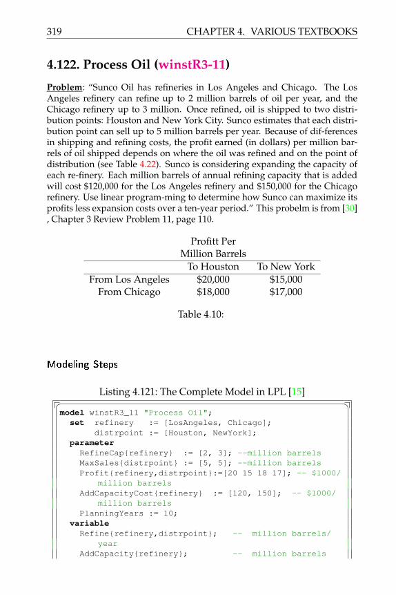
319 CHAPTER 4. VARIOUS TEXTBOOKS

4.122. Process Oil (winstR3-11)

Problem: “Sunco Oil has refineries in Los Angeles and Chicago. The LosAngeles refinery can refine up to 2 million barrels of oil per year, and theChicago refinery up to 3 million. Once refined, oil is shipped to two distri-bution points: Houston and New York City. Sunco estimates that each distri-bution point can sell up to 5 million barrels per year. Because of dif-ferencesin shipping and refining costs, the profit earned (in dollars) per million bar-rels of oil shipped depends on where the oil was refined and on the point ofdistribution (see Table 4.22). Sunco is considering expanding the capacity ofeach re-finery. Each million barrels of annual refining capacity that is addedwill cost $120,000 for the Los Angeles refinery and $150,000 for the Chicagorefinery. Use linear program-ming to determine how Sunco can maximize itsprofits less expansion costs over a ten-year period.” This probelm is from [30], Chapter 3 Review Problem 11, page 110.

Profitt PerMillion Barrels

To Houston To New YorkFrom Los Angeles $20,000 $15,000

From Chicago $18,000 $17,000

Table 4.10:

Modeling Steps

Listing 4.121: The Complete Model in LPL [15]� �model winstR3_11 "Process Oil";

set refinery := [LosAngeles, Chicago];distrpoint := [Houston, NewYork];

parameterRefineCap{refinery} := [2, 3]; --million barrelsMaxSales{distrpoint} := [5, 5]; --million barrelsProfit{refinery,distrpoint}:=[20 15 18 17]; -- $1000/

million barrelsAddCapacityCost{refinery} := [120, 150]; -- $1000/

million barrelsPlanningYears := 10;

variableRefine{refinery,distrpoint}; -- million barrels/

yearAddCapacity{refinery}; -- million barrels

CHAPTER 4. VARIOUS TEXTBOOKS 320

expressionTotalProfitPerYear: sum{refinery, distrpoint} Profit*

Refine;TotalAddCapCost : sum{refinery} AddCapacityCost*

AddCapacity;constraintRefineryLimit{refinery}: sum{distrpoint} Refine <=

RefineCap + AddCapacity;MaxDemand{distrpoint}: sum{refinery} Refine <=

MaxSales;maximize TotalProfit: PlanningYears*TotalProfitPerYear

- TotalAddCapCost;Writep(TotalProfit);

end� �

321 CHAPTER 4. VARIOUS TEXTBOOKS

4.123. Telephone Survey (winstR3-12)

Problem: “For a telephone survey, a marketing research group needs to con-tact at least 150 wives, 120 husbands, 100 single adult males, and 110 singleadult females. It costs $2 to make a daytime call and (because of higher laborcosts) $5 to make an evening call. Table 4.22 lists the results. Because of lim-ited staff, at most half of all phone calls can be evening calls. Formulate anLP to minimize the cost of completing the survey.” This probelm is from [30], Chapter 3 Review Problem 12, page 110.

Percent of Percent ofPerson Daytime Evening

Responding Calls CallsWife 30 30

Husband 10 30Single male 10 15

Single female 10 20None 40 5

Table 4.11:

Modeling Steps

Listing 4.122: The Complete Model in LPL [15]� �model winstR3_12 "Telephone Survey";

set time := [Daytime, Evening];people := [Wife, Husband, SingleMale, SingleFemale];

parameterRespondPercent{people,time}:=[0.3 0.3 0.1 0.3

0.1 .15 0.1 0.2];MustReach{people} := [150, 120, 100, 110];CallCost{time} := [2, 5];

variable Calls{time};constraintContactReq{people}: sum{time} RespondPercent*Calls >=

MustReach;StaffLimit: Calls['Evening']<=1/2*(sum{time} Calls);

minimize TotalCost: sum{time} CallCost*Calls;Writep(TotalCost);

end� �

CHAPTER 4. VARIOUS TEXTBOOKS 322

4.124. Feed Blending (winstR3-13)

Problem: “Feedco produces two types of cattle feed, both consist-ing totallyof wheat and alfalfa. Feed 1 must contain at least 80% wheat, and feed 2 mustcontain at least 60% alfalfa. Feed 1 sells for $1.50/1b, and feed 2 sells for$1.30/1b. Feedco can purchase up to 1000 lb of wheat at 500/1b and up to 800lb of alfalfa at 400/lb. Demand for each type of feed is unlimited. Formulatean LP to maximize Feedco’s profit.” This probelm is from [30] , Chapter 3Review Problem 13, page 110.

Modeling Steps

Listing 4.123: The Complete Model in LPL [15]� �model winstR3_13 "Feed Blending";

setfeed := [f1, f2];grain := [wheat, alfalfa];

parameterMinGrainPct{feed, grain} := [0.80, 0, 0, 0.60];Price{feed} := [1.50, 1.30];GrainCost{grain} := [0.50, 0.40];GrainAvail{grain} := [1000, 800];

variable Produce,P{feed, grain};constraintMinGrain{feed,grain|MinGrainPct>0}: P >= MinGrainPct

*(sum{grain} P);MaxGrain{grain}: sum{feed} P <= GrainAvail;

maximize TotalProfit: sum{feed,grain} Price*P - sum{feed,grain} GrainCost*P;

Writep(TotalProfit,P);end� �

323 CHAPTER 4. VARIOUS TEXTBOOKS

4.125. Feed Blending (winstR3-14)

Problem: “Feedco (see Problem 13) has decided to give its customer (assumeit has only one customer) a quantity discount. If the customer purchases over300 lb of feed 1, each pound over the first 300 lb will sell for only $1.25/1b.Similarly, if the customer purchases more than 300 pounds of feed 2, eachpound over the first 300 lb will sell for $1.00/1b. Modify the LP of Problem13 to account for the presence of quantity discounts. (Hint: Define variablesfor the feed sold at each price.)” This probelm is from [30] , Chapter 3 ReviewProblem 14, page 110.

Modeling Steps

Listing 4.124: The Complete Model in LPL [15]� �model winstR3_14 "Feed Blending";

setfeed := [f1, f2];grain := [Wheat, AlfAlfa];price := [Standard, Discount];

parameterMinGrainPct{feed, grain} := [0.80, 0, 0 , 0.60];FeedPrice{feed,price} := [1.50, 1.25, 1.30, 1.00];GrainCost{grain} := [0.50, 0.40];GrainAvail{grain} := [1000, 800];DiscountCutoff := 300;

variableProduce,P{feed,grain};Sales,S{feed,price};

constraintMinGrain{feed,grain|MinGrainPct>0}: P >= MinGrainPct

*(sum{grain} P);MaxGrain{grain}: sum{feed} P <= GrainAvail;FeedSales{feed}: sum{grain} P >= sum{price} S;SBound: S['Standard'] <= DiscountCutoff;

maximize TotalProfit: sum{feed,price} FeedPrice*S - sum{feed,grain} GrainCost*P;

Writep(TotalProfit,P,S);end� �

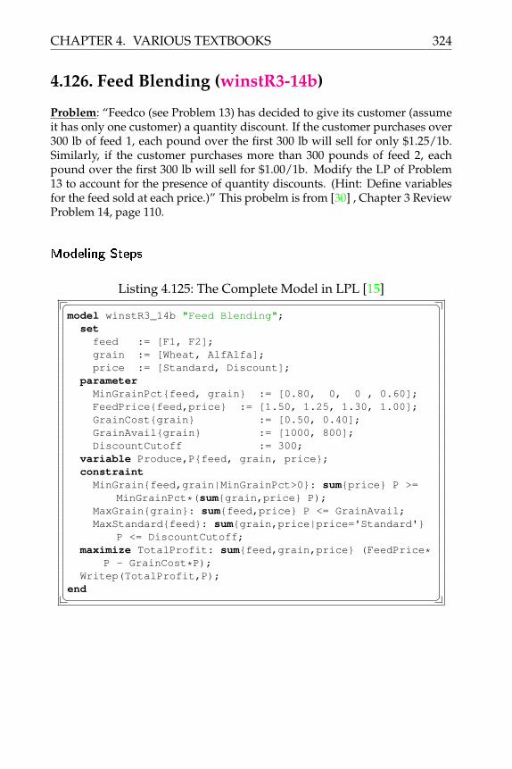
CHAPTER 4. VARIOUS TEXTBOOKS 324

4.126. Feed Blending (winstR3-14b)

Problem: “Feedco (see Problem 13) has decided to give its customer (assumeit has only one customer) a quantity discount. If the customer purchases over300 lb of feed 1, each pound over the first 300 lb will sell for only $1.25/1b.Similarly, if the customer purchases more than 300 pounds of feed 2, eachpound over the first 300 lb will sell for $1.00/1b. Modify the LP of Problem13 to account for the presence of quantity discounts. (Hint: Define variablesfor the feed sold at each price.)” This probelm is from [30] , Chapter 3 ReviewProblem 14, page 110.

Modeling Steps

Listing 4.125: The Complete Model in LPL [15]� �model winstR3_14b "Feed Blending";

setfeed := [F1, F2];grain := [Wheat, AlfAlfa];price := [Standard, Discount];

parameterMinGrainPct{feed, grain} := [0.80, 0, 0 , 0.60];FeedPrice{feed,price} := [1.50, 1.25, 1.30, 1.00];GrainCost{grain} := [0.50, 0.40];GrainAvail{grain} := [1000, 800];DiscountCutoff := 300;

variable Produce,P{feed, grain, price};constraintMinGrain{feed,grain|MinGrainPct>0}: sum{price} P >=

MinGrainPct*(sum{grain,price} P);MaxGrain{grain}: sum{feed,price} P <= GrainAvail;MaxStandard{feed}: sum{grain,price|price='Standard'}

P <= DiscountCutoff;maximize TotalProfit: sum{feed,grain,price} (FeedPrice*

P - GrainCost*P);Writep(TotalProfit,P);

end� �

325 CHAPTER 4. VARIOUS TEXTBOOKS

4.127. Production Planning (winstR3-15)

Problem: “Chemco produces two chemicals: A and B. These chemicals areproduced via two manufacturing processes. Process 1 requires 2 hours oflabor and 1 lb of raw material to produce 2 oz of A and 1 oz of B. Process 2requires 3 hours of labor and 2 lb of raw material to produce 3 oz of A and 2oz of B. Sixty hours of labor and 40 lb of raw material are available. Demandfor A is unlimited, but only 20 oz of B can be sold. A sells for $16/oz, and Bsells for $14/oz. Any B that is unsold must be disposed of at a cost of $2/oz.Formulate an LP to maximize Chemco’s revenue less disposal costs.” Thisprobelm is from [30] , Chapter 3 Review Problem 15, page 110.

Modeling Steps

Listing 4.126: The Complete Model in LPL [15]� �model winstR3_15 "Production Planning";

setchemical := [A, B];process := [1, 2];

parameterLaborReq{process} := [2, 3];RawMatReq{process} := [1, 2];ChemYield{process,chemical} := [2, 1,

3, 2];LaborAvail := 60;RawMatAvail := 40;Price{chemical} := [16.00, 14.00];Demand{chemical} := [-1, 20];DisposeCost{chemical} := [-1, 2.00];

variableProduce{process};Sales{chemical};Dispose{chemical|chemical='B'};

constraintLaborLimit: sum{process} LaborReq*Produce <=

LaborAvail;RawMatLimit: sum{process} RawMatReq*Produce <=

RawMatAvail;ProcessBalance{chemical}: sum{process} ChemYield*

Produce = Sales + Dispose;MaxDemand: Sales['B'] <= Demand['B'];

maximize TotalProfit: sum{chemical} Price*Sales- sum{chemical} DisposeCost*Dispose;

Writep(TotalProfit,Produce,Sales,Dispose);end� �

CHAPTER 4. VARIOUS TEXTBOOKS 326

4.128. Product Mix (winstR3-17)

Problem: “Furnco manufactures tables and chairs. Each table and chair mustbe made entirely out of oak or entirely out of pine. A total of 150 board ft ofoak and 210 board ft of pine are available. A table requires either 17 boardft of oak or 30 board ft of pine, and a chair requires either 5 board ft of oakor 13 board ft of pine. Each table can be sold for $40, and each chair for $15.Formulate an LP that can be used to maximize revenue.” This probelm isfrom [30] , Chapter 3 Review Problem 17, page 110.

Modeling Steps

Listing 4.127: The Complete Model in LPL [15]� �model winstR3_17 "Product Mix";

setfurniture := [desk, chair];materials := [oak, pine];

parameterMatAvail{materials} := [150, 210];MatUsed{furniture, materials} := [17, 30, 5, 13];Price{furniture} := [40.00, 15.00];

variable Produce{furniture};constraint MatReq{materials}: sum{furniture} MatUsed*

Produce <= MatAvail;maximize TotalProfit: sum{furniture} Price*Produce ;Writep(TotalProfit);

end� �

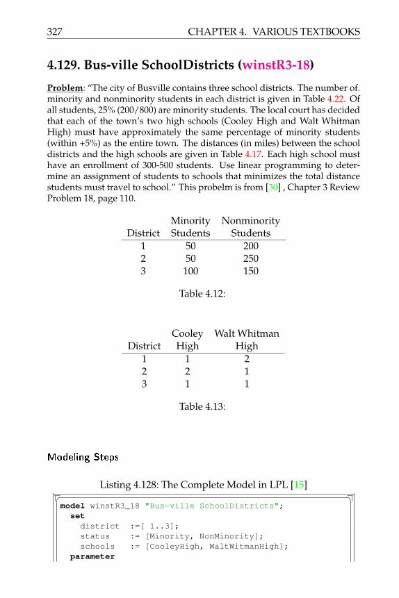
327 CHAPTER 4. VARIOUS TEXTBOOKS

4.129. Bus-ville SchoolDistricts (winstR3-18)

Problem: “The city of Busville contains three school districts. The number of.minority and nonminority students in each district is given in Table 4.22. Ofall students, 25% (200/800) are minority students. The local court has decidedthat each of the town’s two high schools (Cooley High and Walt WhitmanHigh) must have approximately the same percentage of minority students(within +5%) as the entire town. The distances (in miles) between the schooldistricts and the high schools are given in Table 4.17. Each high school musthave an enrollment of 300-500 students. Use linear programming to deter-mine an assignment of students to schools that minimizes the total distancestudents must travel to school.” This probelm is from [30] , Chapter 3 ReviewProblem 18, page 110.

Minority NonminorityDistrict Students Students

1 50 2002 50 2503 100 150

Table 4.12:

Cooley Walt WhitmanDistrict High High

1 1 22 2 13 1 1

Table 4.13:

Modeling Steps

Listing 4.128: The Complete Model in LPL [15]� �model winstR3_18 "Bus-ville SchoolDistricts";

setdistrict :=[ 1..3];status := [Minority, NonMinority];schools := [CooleyHigh, WaltWitmanHigh];

parameter

CHAPTER 4. VARIOUS TEXTBOOKS 328

StudentCount{district,status} := [ 50, 200, 50, 250,100, 150];

Distance{district,schools} := [1, 2, 2, 1, 1, 1];MinorityPercent := 0.25;MinMinority := MinorityPercent - 0.05;MaxMinority := MinorityPercent + 0.05;MinStudents := 300;MaxStudents := 500;

variable AssignStudents,A{district,schools,status};constraintStudentAssignment{district,status}: sum{schools} A =

StudentCount;StudentLimit{schools}: MinStudents <= sum{district,

status} A <= MaxStudents;MinorityLowerLimit{schools}: sum{district,status|

status='Minority'} A>= MinMinority*(sum{district,status} A);

MinorityUpperLimit{schools}: sum{district,status|status='Minority'} A

<= MaxMinority*(sum{district,status} A);minimize TotalDistance: sum{district,schools,status}

Distance*A;Writep(TotalDistance);

end� �

329 CHAPTER 4. VARIOUS TEXTBOOKS

4.130. Brady (winstR3-19)

Problem: “Brady Corporation produces cabinets. Each week, they require90,000 cu ft of processed lumber. They may obtain lumber in two ways. First,they may purchase lumber from an outside supplier and then dry it at theirkiln. Sec-ond, they may chop down logs on their land, cut them into lumberat their sawmill, and finally dry the lumber at their kiln. Brady can purchasegrade 1 or grade 2 lumber. Grade l lumber costs $3 per cu ft and when driedyields 0.7 cu ft of useful lumber. Grade 2 lumber costs $7 per cubic foot andwhen dried yields 0.9 cu ft of useful lumber. It costs the Company $3 to chopdown a log. After being cut and dried, a log yields 0.8 cu ft of lumber. Bradyincurs costs of $4 per cu ft of lumber dried. It costs $2.50 per cu ft of logs sentthrough the sawmill. Each week, the sawmill can process up to 35,000 cu ftof lumber. Each week, up to 40,000 cu ft of grade 1 lumber and up to 60,000cu ft of grade 2 lumber can be purchased. Each week, 40 hours of time areavailable for drying lumber. The time it takes to dry 1 cu ft of grade 1 lumber,grade 2 lumber, or logs is as follows: grade 1-2 seconds; grade 2-0.8 second;log 1.3 seconds. Formulate a.11 LP to help Brady minimize the weekly costof meeting the demand for processed lumber.” This probelm is from [30] ,Chapter 3 Review Problem 19, page 111.

Modeling Steps

Listing 4.129: The Complete Model in LPL [15]� �model winstR3_19 "Brady";

setlumber := [outside, own, log];grade := [g1, g2];

parameterPrice{grade} := [3.00, 7.00];Yield{lumber} := [0.7, 0.9, 0.8];ChopCost := 3.00;DryCost := 4.00;

-- model not finishedWrite('The model is not complete\n');

end� �

CHAPTER 4. VARIOUS TEXTBOOKS 330

4.131. Canadian Parks Commission (winstR3-20)

Problem: “The Canadian Parks Commission controls two tracts of land. Tract1 consists of 300 acres and tract 2, 100 acres. Each acre of tract 1 can be usedfor spruce trees or hunting, or both. Each acre of tract 2 can be used for sprucetrees or camping, or both. The capital (in hundreds of dollars) and labor (inman-days) required to maintain one acre of each tract, and the profit (in thou-sands of dollars) per acre for each possible use of land are given in Table 4.22.Capital of $150,000 and 200 man-days of labor are available. How should theland be allocated to various uses to maximize profit received from the twotracts?” This probelm is from [30] , Chapter 3 Review Problem 20, page 111.

Capital Labor ProfitTract 1 Spruce 3 0.1 0.2Tract 1 Hunting 3 0.2 0.4Tract 1 Both 4 0.2 0.5Tract 2 Spruce 1 0.05 0.06Tract 2 Camping 30 5 0.09Tract 2 Both 10 1.01 1.1

Table 4.14:

Modeling Steps

Listing 4.130: The Complete Model in LPL [15]� �model winstR3_20 "Canadian Parks Commission";

set Land := [Tract1, Tract2];UsedFor:=[Spruce Hunting SpruceHunt Camping

SpruceCamp];parameterAcresAvail{Land} := [300, 100];

/* CapitalUse{Land,UsedFor} :=[300 300 400 0 0 100 0 0 3000 1000];

LaborUse{Land,UsedFor} :=[.1 .2 .2 0 0 .05 0 0 5 1.01];

Profit{Land,UsedFor} :=[200 400 500 0 0 60 0 0 90 1100]; */

CapitalUse{Land,UsedFor}:= /Tract1 Spruce 300,Tract1 Hunting 300, Tract1 SpruceHunt 400,Tract2 Spruce 100, Tract2 Camping 3000,Tract2 SpruceCamp 1000/;

LaborUse{Land,UsedFor}:= /Tract1 Spruce 0.1,

331 CHAPTER 4. VARIOUS TEXTBOOKS

Tract1 Hunting 0.2, Tract1 SpruceHunt 0.2,Tract2 Spruce 0.05, Tract2 Camping 5.0,Tract2 SpruceCamp 1.01/;

Profit{Land,UsedFor}:= /Tract1 Spruce 200,Tract1 Hunting 400, Tract1 SpruceHunt 500,Tract2 Spruce 60, Tract2 Camping 90,Tract2 SpruceCamp 1100/;

CapitalAvail := 150000; LaborAvail := 200;variable Allocate{Land,UsedFor};constraintAcresLimit{Land}: sum{UsedFor} Allocate<=AcresAvail;CapitalLimit: sum{Land, UsedFor} CapitalUse*Allocate

<= CapitalAvail;LaborLimit: sum{Land, UsedFor} LaborUse*Allocate <=

LaborAvail;maximize TotalProfit:sum{Land,UsedFor} Profit*Allocate;Writep(TotalProfit);

end� �

CHAPTER 4. VARIOUS TEXTBOOKS 332

4.132. Chandler Enterprises (winstR3-21)

Problem: “Chandler Enterprises produces two competing prod-ucts: A and B.The company wants to sell these products to two groups of customers: group1 and group 2. The value each customer places on a unit of A and B is asshown in Table 4.22. Each customer will buy either product A or product B,but not both. A customer is willing to buy product A if she believes that Valueof product A - price of product A ≥ Value of product B - price of product Band Value of product A - price of product A ≥ 0. A customer is willing to buyproduct B if she believes that Value of product B - price of product B ≥ valueof product A - price of product A and Value of product B - price of product B≥ 0.

Group 1 has 1000 members, and group 2 has 1500 members. Chandler wantsto set prices for each product that ensure that group 1 members purchaseproduct A and group 2 members purchase product B. Formulate an LP thatwill help Chandler maximize revenues.” This problem is from [30] , Chapter3 Review Problem 21, page 111.

Modeling Steps

Group 1 Group 2Customer Customer

Value of A to $10 $12Value of B to $8 $15

Table 4.15:

Listing 4.131: The Complete Model in LPL [15]� �model winstR3_21 "Chandler Enterprises";

set product := [A, B];custgroup := [1..2];

parameter Value{product,custgroup}:=[10 12 8 15];Members{custgroup} := [1000, 1500];

variable Price{product};constrainta: Value['A','1'] - Price['A'] >= Value['B','1'] -

Price['B'];b: Value['B','2'] - Price['B'] >= Value['A','2'] -

Price['A'];c: Value['A','1'] - Price['A'] >= 0;d: Value['B','2'] - Price['B'] >= 0;

333 CHAPTER 4. VARIOUS TEXTBOOKS

maximize TotalRevenues: Members['1']*Price['A'] +Members['2']*Price['B'];

Writep(TotalRevenues);end� �

CHAPTER 4. VARIOUS TEXTBOOKS 334

4.133. Alden Enterprices (winstR3-22)

Problem: “Alden Enterprises produces two products. Each prod-uct can beproduced on one of two machines. The length of time needed to produce eachproduct (in hours) on each machine is as shown in Table 4.22. Each month,500 hours of time are available on each machine. Each month, customers arewilling to buy up to the quantities of each product at the prices given in Table4.17. The company’s goal is to maximize the revenue obtained from sellingunits during the next two months. Formulate an LP to help meet this goal.”This problem is from [30] , Chapter 3 Review Problem 22, page 112.

Machine 1 Machine 2Product 1 4 3Product 2 7 4

Table 4.16:

Demand PricesMonth 1 Month 2 Month 1 Month 2

Product 1 100 190 $55 $12Product 2 140 130 $65 $32

Table 4.17:

Modeling Steps

Listing 4.132: The Complete Model in LPL [15]� �model winstR3_22 "Alden Enterprices";

set product := [p1,p2];machine := [m1,m2];month := [Jan,Feb];

parameter TimeAvail{machine} := [500, 500];MachineTime{product,machine} := [4, 3, 7, 4];Price{product, month} := [55 12 65 32];Demand{product, month} := [100, 190, 140, 130];

variable Produce{product, machine, month};constraintTimeCapacity{machine}: sum{product,month} MachineTime

*Produce <= TimeAvail;MaxDemand{product,month}: sum{machine} Produce <=

Demand;

335 CHAPTER 4. VARIOUS TEXTBOOKS

maximize TotalRevenue: sum{product,machine,month} Price

*Produce;Writep(TotalRevenue);

end� �

CHAPTER 4. VARIOUS TEXTBOOKS 336

4.134. Kiriakis (winstR3-23)

Problem: “Kiriakis Electronics produces three products. Each product mustbe processed on each of three types of ma-chines. When a machine is inuse, it must be manned by a worker. The time (in hours) required to processeach product on each machine and the profit associated with each product areshown in Table 4.22. At present, five type 1 machines, three type 2 machines,and four type 3 machines are available. The company has ten workers avail-able and must determine how many workers to assign to each machine. Theplant is open 40 hours per week, and each worker works 35 hours per week.Formulate an LP that will enable Kiriakis to assign workers to machines ina way that maximizes weekly profits. (Note: A worker need not spend theentire work week manning a single machine.)” This probelm is from [30] ,Chapter 3 Review Problem 23, page 112.

Product 1 Product 2 Product 3Machine 1 2 3 4Machine 2 3 5 6Machine 3 4 7 9Profit $6 $8 $10

Table 4.18:

Modeling Steps

Listing 4.133: The Complete Model in LPL [15]� �model winstR3_23 "Kiriakis";

set p := [1..3] "Products";m := [1..3] "Machines";w := [1..10] "Workers";

parameter ProcessTime{m,p}:=[2 3 4 3 5 6 4 7 9];Profit{p} := [6, 8, 10];MachineAvail{m} := [5, 3, 4];PlantOpenHours := 40;WorkerHours := 35;

variableProduce,P{p};MachineHours,M{m};

constraintProcessLimit{m}: sum{p} ProcessTime*P<=MachineHours;MachineLimit{m}: M <= PlantOpenHours*MachineAvail;WorkerLimit: sum{m} M <= 10*WorkerHours;

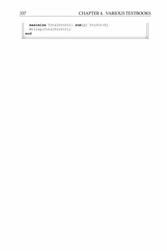
337 CHAPTER 4. VARIOUS TEXTBOOKS

maximize TotalProfit: sum{p} Profit*P;Writep(TotalProfit);

end� �

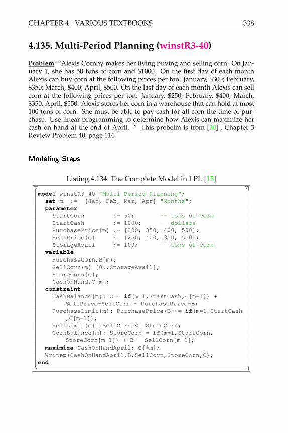
CHAPTER 4. VARIOUS TEXTBOOKS 338

4.135. Multi-Period Planning (winstR3-40)

Problem: “Alexis Cornby makes her living buying and selling corn. On Jan-uary 1, she has 50 tons of corn and $1000. On the first day of each monthAlexis can buy corn at the following prices per ton: January, $300; February,$350; March, $400; April, $500. On the last day of each month Alexis can sellcorn at the following prices per ton: January, $250; February, $400; March,$350; April, $550. Alexis stores her corn in a warehouse that can hold at most100 tons of corn. She must be able to pay cash for all corn the time of pur-chase. Use linear programming to determine how Alexis can maximize hercash on hand at the end of April. ” This probelm is from [30] , Chapter 3Review Problem 40, page 114.

Modeling Steps

Listing 4.134: The Complete Model in LPL [15]� �model winstR3_40 "Multi-Period Planning";

set m := [Jan, Feb, Mar, Apr] "Months";parameterStartCorn := 50; -- tons of cormStartCash := 1000; -- dollarsPurchasePrice{m} := [300, 350, 400, 500];SellPrice{m} := [250, 400, 350, 550];StorageAvail := 100; -- tons of corn

variablePurchaseCorn,B{m};SellCorn{m} [0..StorageAvail];StoreCorn{m};CashOnHand,C{m};

constraintCashBalance{m}: C = if(m=1,StartCash,C[m-1]) +

SellPrice*SellCorn - PurchasePrice*B;PurchaseLimit{m}: PurchasePrice*B <= if(m=1,StartCash

,C[m-1]);SellLimit{m}: SellCorn <= StoreCorn;CornBalance{m}: StoreCorn = if(m=1,StartCorn,

StoreCorn[m-1]) + B - SellCorn[m-1];maximize CashOnHandApril: C[#m];Writep(CashOnHandApril,B,SellCorn,StoreCorn,C);

end� �

339 CHAPTER 4. VARIOUS TEXTBOOKS

4.136. Production Planning (winstR3-40b)

Problem: “Alexis Cornby makes her living buying and selling corn. On Jan-uary 1, she has 50 tons of corn and $1000. On the first day of each monthAlexis can buy corn at the following prices per ton: January, $300; February,$350; March, $400; April, $500. On the last day of each month Alexis can sellcorn at the following prices per ton: January, $250; February, $400; March,$350; April, $550. Alexis stores her corn in a warehouse that can hold at most100 tons of corn. She must be able to pay cash for all corn the time of pur-chase. Use linear programming to determine how Alexis can maximize hercash on hand at the end of April. ” This probelm is from [30] , Chapter 3Review Problem 40, page 114.

Modeling Steps

Listing 4.135: The Complete Model in LPL [15]� �model winstR3_40b "Production Planning";

set m := [Jan, Feb, Mar, Apr];parameterStartCorn := 50;

-- tons of cormStartCash := 1000;

-- dollarsPurchasePrice{m} := [300, 350, 400, 500];SellPrice{m} := [250, 400, 350, 550];StorageAvail := 100;

-- tons of cornvariablePurchaseCorn,B{m};SellCorn{m};StoreCorn{m} [0..StorageAvail];CashOnHand,C{m};

constraintCashBalance{m}: C = if(m=1,StartCash,C[m-1]) +

SellPrice*SellCorn - PurchasePrice*B;PurchaseLimit{m}: PurchasePrice*B <= if(m=1,StartCash

,C[m-1]);SellLimit{m}: SellCorn <= StoreCorn;CornBalance{m}: StoreCorn = if(m=1,StartCorn,

StoreCorn[m-1]) + B - SellCorn[m-1];maximize CashOnHandApril: C[#m];Writep(CashOnHandApril,B,SellCorn,StoreCorn,C);

end� �

CHAPTER 4. VARIOUS TEXTBOOKS 340

4.137. Multi-Period Finance Planning (winstR3-41)

Problem: “At the beginning of month 1, Finco has $400 in cash. At the be-ginning of months 1, 2, 3, and 4. Finco rcceives certain revenues, after whichit pays hills (see Table 4.22). Any money left over may be invested for onemonth at the interest rate of 0.1% per month; for two months at 0.5% permonth; for three months at 1 % per month; or for four months at 2% permonth. Use linear programming to determine an invest ment strategy thatmaximizes cash on hand at the beinning of month 5.” This probelm is from[30] , Chapter 3 Review Problem 41, page 114.

Revenue BillsMonth 1 $400 $600Month 2 $800 $500Month 3 $300 $500Month 4 $300 $250

Table 4.19:

Modeling Steps

Listing 4.136: The Complete Model in LPL [15]� �model winstR3_41 "Multi-Period Finance Planning";

set period ,p :=[ 1..4];parameterStartCash := 400;Interest{p} := [0.001, 0.005, 0.01, 0.02];Revenues{p} := [400, 800, 300, 300];Bills{p} := [600, 500, 500, 250];

variableInvest{p};Cash{p};

constraint Balance{p}: Cash + Bills + Invest= if(p=1,StartCash,Cash[p-1]) + Revenues + (1+

Interest)*Invest[p-1];maximize EndCash: Cash[#p];Writep(EndCash,Invest,Cash);

end� �

341 CHAPTER 4. VARIOUS TEXTBOOKS

4.138. Transporation: Waste disposal (winstR3-42)

Problem: “City 1 produces 500 tons of waste per day, and city produces 400tons of waste per day. Waste must be incinerated at incinerator 1 or 2, andeach incinerator can process up to 500 tons of waste per day. The cost toincinerate waste is $40/ton at incinerator 1 and $30/ton at 2. Incinerationreduces each ton of waste to 0.2 tons of debris, which must be dumped atone of two landfills. Each landfill can receive at most 200 tons of debris perday. It costs $3 per mile to trans-port a ton of material (either debris or waste).Distances (in miles) between locations are shown in Table 4.22. Formulate anLP that can be used to minimize the total cost of disposing of the waste ofboth cities.” This probelm is from [30] , Chapter 3 Review Problem 42, page114.

Incinerator 1 Incinerator 2City 1 30 5City 2 36 42

Landfill 1 Landfill 2Incinerator 1 5 8Incinerator 2 9 6

Table 4.20:

Modeling Steps

Listing 4.137: The Complete Model in LPL [15]� �model winstR3_42 "Transporation: Waste disposal";

setcity := [1..2];incin := [1..2];landfill := [1..2];

parameterWasteProduced{city} := [500, 400];BurnCapacity{incin} := [500, 500];BurnCost{incin} := [40, 30];ResultingDebris := 0.20;LandfillCapacity{landfill} := [200, 200];CostPerMile := 3.00;DistToIncin{city,incin} := [30, 5, 36, 42];DistToLandfill{incin,landfill} := [5, 8, 9, 6];

variableWasteToIncin,W{city,incin};

CHAPTER 4. VARIOUS TEXTBOOKS 342

DebrisToLandfill,D{incin,landfill};expressionTotalBurnCost : sum{city,incin} BurnCost*W;IncinTranspCost : CostPerMile*(sum{city,incin}

DistToIncin*W);LandfillTranspCost: CostPerMile*(sum{incin,landfill}

DistToLandfill*D);constraintBurnWaste{city}: sum{incin} W = WasteProduced;IncinLimit{incin}: sum{city} W <= BurnCapacity;IncinBalance{incin}: sum{city} W = 1/ResultingDebris

*(sum{landfill} D);LandfillLimit{landfill}: sum{incin} D <=

LandfillCapacity;minimize TotalCost: TotalBurnCost + IncinTranspCost +

LandfillTranspCost;Writep(TotalCost);

end� �

343 CHAPTER 4. VARIOUS TEXTBOOKS

4.139. Product-mix with blending (winstR3-45)

Problem: “Turkeyco produces two types of turkey cutlets for sale to fast foodrestaurants. Each type of cutlet consists of white meat and dark meat. Cutlet1 sells for $4/lb and must consist of at least 70% white meat. Cutlet 2 sells for$3/lb and must consist of at least 60% white meat. At most 50 lb of cutlet 1and 30 lb of cutlet 2 can be sold. The two types of turkey used to manufacturethe cutlets are purchased from the Gob-bleGobble Turkey Farm. Each type 1turkey costs $10 and yields 5 lb of white meat and 2 lb of dark meat. Eachtype 2 turkey costs $8 and yields 3 lb of white meat and 3 lb of dark meat.Formulate an LP to maximize Turkeyco’s profit.” This probelm is from [30] ,Chapter 3 Review Problem 45, page 115.

Modeling Steps

Listing 4.138: The Complete Model in LPL [15]� �model winstR3_45 "Product-mix with blending";

setc := [1..2] "Cutlet";m := [White, Dark] "Meat";t := [1..2] "Turkey";

parameterPrice{c} := [4.00, 3.00];MinWhitePercent{c} := [0.70, 0.60];MaxDemand{c} := [50, 30];TurkeyCost{t} := [10.00, 8.00];TurkeyMeat{t, m} := [5, 2, 3, 3];

variablePurchaseTurkey{t};CutletMeat{c,m};

expressionTotalRevenue: sum{c,m} Price*CutletMeat;TotalCost : sum{t} TurkeyCost*PurchaseTurkey;

constraintMinWhiteMeat{c}: sum{m|m='White'} CutletMeat >=

MinWhitePercent*(sum{m} CutletMeat);MaximumDemand{c}: sum{m} CutletMeat <= MaxDemand;MeatLimit{m}: sum{c} CutletMeat <= sum{t} TurkeyMeat*

PurchaseTurkey;maximize TotalProfit: TotalRevenue - TotalCost;Writep(TotalProfit);

end� �

CHAPTER 4. VARIOUS TEXTBOOKS 344

4.140. Review Prob (Priceler) (winstR3-46)

Problem: “Priceler manufactures sedans and wagons. The number of vehiclesthat can be sold each of the next three months are listed in Table 4.22. Eachsedan sells for $8000, and each wagon sells for $9000. It costs $6000 to producea sedan and $7500 to produce a wagon. To hold a vehicle in inventory for onemonth costs $150 per sedan and $200 per wagon. During each month, atmost 1500 vehicles can be produced. Production line restrictions dictate thatduring month 1, at least two thirds of all cars produced must be sedans. At thebeginning of month 1, 200 sedans and 100 wagons are available. Formulatean LP that can be used to maximize Priceler’s profit during the next threemonths.” This probelm is from [30] , Chapter 3 Review Problem 46, page 116.

Sedans WagonsMonth 1 1100 600Month 2 1500 700Month 3 1200 500

Table 4.21:

Modeling Steps

Listing 4.139: The Complete Model in LPL [15]� �model winstR3_46 "Review Prob (Priceler)";

set v := [Sedan, Wagon] "Vehicles";m :=[ 1..3] "Months";

parameter Price{v} := [8000, 9000];ProdCost{v} := [6000, 7500];InvtCost{v} := [150, 200];InvtCapacity := 1500;StartInvt{v} := [200, 100];Demand{m, v} := [1100, 600, 1500, 700, 1200, 500];

variableProduce,P{v,m};Inventory,I{v,m};Sales,S{v,m} [0..Demand];

expressionTotalRevenue : sum{v,m} Price*S;TotalProdCost: sum{v,m} ProdCost*P;TotalInvtCost: sum{v,m} InvtCost*I;TotalCost : TotalProdCost+TotalInvtCost;

constraintInventoryBalance{v,m}:I=if(m=1,StartInvt,I[m-1])+P-S;

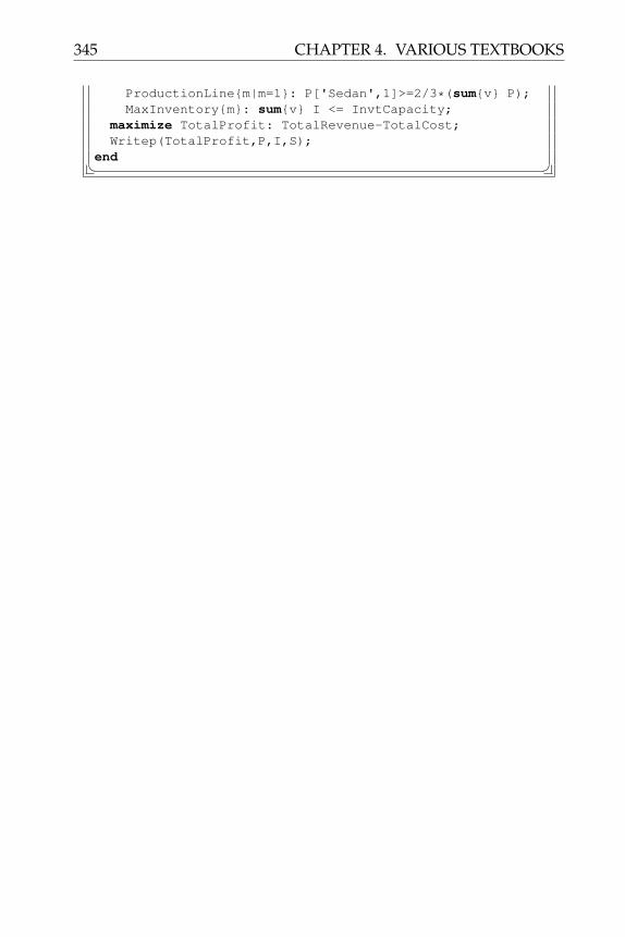
345 CHAPTER 4. VARIOUS TEXTBOOKS

ProductionLine{m|m=1}: P['Sedan',1]>=2/3*(sum{v} P);MaxInventory{m}: sum{v} I <= InvtCapacity;

maximize TotalProfit: TotalRevenue-TotalCost;Writep(TotalProfit,P,I,S);

end� �

CHAPTER 4. VARIOUS TEXTBOOKS 346

4.141. EJ-Korvair DeptStore (winstR3-53)

Problem: “E.J. Korvair Department Store has $1000 in available cash. At thebeginning of each of the next six months, E.J. will receive revenues and paybills as shown in Table 4.22. It is clear that E.J. will have a short-term cash flowproblem until the store receives revenues from the Christmas shopping sea-son. To solve this problem, E.J. must borrow money. At the beginning of July,E.J. may take out a six-month loan. Any money borrowed for a six-month pe-riod must be paid back at the end of December along with 9% interest (earlypayback does not reduce the interest cost of the loan). E.J. may also meetcash needs through month-to-month bor- rowing. Any money borrowed fora one-month period incurs an interest cost of 4% per month. Use linear pro-gramming to determine how E.J. can minimize the cost of paying its bills ontime.” This probelm is from [30] , Chapter 3 Review Problem 53, page 117.

Revenues BillsJuly $1000 $5000August $2000 $5000September $2000 $6000October $4000 $2000November $7000 $2000December $9000 $1000

Table 4.22:

Modeling Steps

Listing 4.140: The Complete Model in LPL [15]� �model winstR3_53 "EJ-Korvair DeptStore";

set m := [July, August, September, October, November,December] "Months";

parameterCashAvail := 1000;Revenues{m} := [1000, 2000, 2000, 4000, 7000, 9000];Bills{m} := [5000, 5000, 6000, 2000, 2000, 1000];LoanInterest := 0.09;BorrowInterest := 0.04;LoanRate := 1.0 + LoanInterest;BorrowRate := 1.0 + BorrowInterest;

variableCashLevel,C{m};SixMonthLoan,L;

347 CHAPTER 4. VARIOUS TEXTBOOKS

BorrowMonth,S{m};constraintCashBalance{m|m=1}:

C = CashAvail + Revenues - Bills + S + L;CashBalance1{m|m>1 and m<#m}:

C = C[m-1] + Revenues - Bills + S - BorrowRate*S[m-1];

CashBalance2{m|m=#m}:C = C[m-1] + Revenues - Bills - BorrowRate*S[m-1]

- LoanRate*L;minimize TotalCost: LoanInterest*L + sum{m}

BorrowInterest*S;Writep(TotalCost);

end� �

CHAPTER 5

MODELS FROM THE GAMSLIBRARY

5.1. Linear Quadratic Control Problem (abel)

Problem: Linear Quadratic Riccati Equations are solved as a General Nonlin-ear Programming Problem instead of the usual Matrix Recursion.

This model is from the GAMS model library (GAMS SEQ=64). See also [17]

Modeling Steps

Listing 5.1: The Complete Model in LPL [15]� �model ABEL "Linear Quadratic Control Problem";

set n,np "states" :=[consumpt, invest];m,mp "controls":=['gov-expend', money];k "horizon" :=['1964-i' '1964-ii' '1964-iii'

'1964-iv' '1965-i' '1965-ii' '1965-iii' '1965-iv'];parametera{n,np} "state vector matrix" := [0.914 -0.016,

0.097 0.424];b{n,m} "control vector matrix" := [0.305 0.424,

-0.101 1.459];wk{n,np}"penalty matrix for states - input" :=

[0.0625 ., . 1];lambda{m,mp} "penalty matrix for comtrols" := [1 .,

. 0.444];c{n} "constant term" := [-59.4, -184.7 ];xinit{n} "initial value" := [387.9, 85.3 ];uinit{m} "initial controls" := [110.5, 147.1];xtilde{n,k} "desired path for x" := xinit*1.0075^(k

-1);utilde{m,k} "desired path for u" := uinit*1.0075^(k

-1);

349

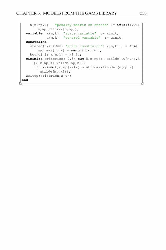
CHAPTER 5. MODELS FROM THE GAMS LIBRARY 350

w{n,np,k} "penalty matrix on states" := if(k<#k,wk[n,np],100*wk[n,np]);

variable x{n,k} "state variable" := xinit;u{m,k} "control variable" := uinit;

constraintstateq{n,k|k<#k} "state constraint": x[n,k+1] = sum{

np} a*x[np,k] + sum{m} b*u + c;bound{n}: x[n,1] = xinit;

minimize criterion: 0.5*(sum{k,n,np}(x-xtilde)*w[n,np,k]*(x[np,k]-xtilde[np,k]))+ 0.5*(sum{k,m,mp|k<#k}(u-utilde)*lambda*(u[mp,k]-

utilde[mp,k]));Writep(criterion,x,u);

end� �

351 CHAPTER 5. MODELS FROM THE GAMS LIBRARY

5.2. Agreste Farm Level Model of NE Brazil(agreste)

Problem: This is a farm level model of the north east region of brazil. Thereis only one farm type - medium sized. There are 3 types of land and risk onrevenue is considered.

This model is from teh GAMS model library (GAMS SEQ=88). See also [20]

Modeling Steps

Listing 5.2: The Complete Model in LPL [15]� �model AGRESTE "Agreste Farm Level Model of NE Brazil";set c "crops" := [

cotton_h banana sugar_cane beans_arrbeans_cor oranges manioc corn sisal];

tm "months" := [ jan, feb, mar, apr, may, jun, jul,aug, sep, oct, nov, dec ];

p "cropping activities" := [crop_02 -- cotton_herbaceocrop_05 -- bananacrop_10 -- sugar canecrop_15 -- orangescrop_16 -- manioccrop_17 -- corncrop_19 -- sisalcrop_25 -- beans-de-corda corncrop_29 -- cotton_herbaceo beans-de-

arranca corncrop_30 -- cotton_herbaceo beans-de-

corda corncrop_33 -- beans-de-arranca corncrop_36 -- beans-de-arranca manioc corn

];s,sp "land types" := [

good --flat and near water or humid and low lyingmedium -- hilly or more arid than goodpasture -- cultivated pasture or tree crops

];sc{s} "crop lands" := [ good , medium ];r "livestock feeding alternatives" := [

rec_1 rec_2 rec_3 ];ty "year" := [ 1960..1969 ];dr "family consumption bundle alternatives

" := [ one , two , three ];km "technology characteristics" := [

CHAPTER 5. MODELS FROM THE GAMS LIBRARY 352

equipment, fertilizer, seeds, sprouts,itech ];

parameterlandc{s} "land data (ha)" := / good 8.775, medium

11.64, pasture 21.92/;rations{r} "lvstk rations feeding alternative (cr

per head)":= / rec_1 5.141 , rec_2 21.646 ,rec_3 49.845/;

xcropl{p,s} "limits on cropping activities" := /crop_19 good 0.036, crop_19 medium 0.298/;

ldp{s,s} "land downgrading possibilities" := /:good medium:

good 1 .medium -1 1pasture . -1 /;

/* land req for lvstk seems high but ok - pg 65 para 3 */lio{s,r} "land requirements for lvstk feed

alternatives (ha per head)" := /:rec_1 rec_2 rec_3:

medium 1.407 0.611 0.631pasture 0.209 2.03 0.9 /;

labor{p,tm} "labor requirements for cropping (mandaysper ha)" := /

:jan feb mar apr may jun julaug sep oct nov dec:

crop_02 4.79 10.89 18.70 9.83 8.03 20.95 15.6715.48 11.35 8.38 8.23 4.54

crop_05 8.24 0.89 5.43 3.31 11.13 10.33 3.272.65 5.47 3.67 3.18 1.44

crop_10 5.78 3.37 4.03 7.09 4.64 5.91 7.679.23 5.93 9.05 7.59 6.37

crop_15 2.00 2.36 4.13 2.13 7.18 5.88 3.219.20 6.89 3.30 9.70 8.87

crop_16 5.71 7.60 7.28 8.15 8.48 10.71 9.3412.76 8.93 10.22 6.18 8.34

crop_17 9.19 14.42 10.59 12.01 3.47 10.75 5.887.30 4.14 4.25 3.49 2.11

crop_19 1.22 1.11 0.56 0.78 1.19 0.44 1.893.04 2.93 4.99 7.73 9.44

crop_25 12.46 11.35 24.38 22.03 16.91 9.47 10.979.70 4.93 6.41 0.53 0.89

crop_29 5.54 10.30 9.24 8.97 15.82 13.00 14.7410.64 5.64 4.90 4.73 4.92

crop_30 9.18 3.94 16.15 23.69 28.12 20.58 17.7315.06 4.58 9.76 7.39 2.67

crop_33 6.87 10.19 10.61 9.14 18.38 11.50 9.2213.36 3.85 3.87 2.65 1.09

crop_36 7.44 10.21 9.63 16.18 20.11 16.86 14.8614.00 8.04 6.69 5.49 5.26 /;

353 CHAPTER 5. MODELS FROM THE GAMS LIBRARY

llab{tm,r} "labor requirement for lvstk feed (mandaysper head)" := /

:rec_1 rec_2 rec_3:jan 4.261 1.873 1.933feb 2.854 1.262 1.302mar 0.040 0.040 0.040apr 0.040 0.040 0.040may 0.040 0.040 0.040jun 0.040 0.040 0.040jul 0.040 0.040 0.040aug 0.040 0.040 0.040sep 0.040 0.040 0.040oct 0.040 0.040 0.040nov 7.075 3.095 3.195dec 7.075 3.095 3.195/;

cbndl{c,dr} "consumption bundles (tons per bundle)" :=/

:one two three:beans_arr 0.225 0.152 0.15manioc 0.965 2.64 0.935corn 0.235 0.232 0.581 /;

crev{c,ty} "crop revenue time series (cr per ha)" := /:1960 1961 1962 1963 1964 1965 1966 1967

1968 1969:banana 6399 8193 9215 8581 7988 7228 5923 6738

7221 7842sugar_cane 1667 1899 1898 2230 2265 2067 1499 1903

1901 1929beans_cor 546 585 1091 651 470 621 605 518

519 772manioc 986 1543 2658 1639 1146 1380 1357 1702

1560 1580corn 267 378 544 329 320 351 310 322

294 349 /;price{c} "crop reference prices (cr per kg)" := /cotton_h 1.9 banana 4 sugar_cane 35beans_arr 2.5 beans_cor 1.5 oranges 10manioc 0.17 corn 0.15 sisal 1 /;/* wage data: pg 159, working capital: is this correct

: =6.4*1113, family labor available: correct? */fwage "family reservation wage rate (cr/man-month)"

:= 75;twage "temporary labor wage rate (cr/man-month)" :=

250;pwage "permanent labor wage rate (cr/man-year)"

:=2054;vsc "value of self-consumption (cr/bundle)" :=

934;wcbar "working capital (cr)"

:=7123.2;

CHAPTER 5. MODELS FROM THE GAMS LIBRARY 354

famlab "family labor man equivalent wrks)" :=70.5;

lprice "livestock price (cr per head)" :=211;

vetpr "cost of vetinanry servic per head)" :=1;

dpm "man days per man month" :=25;

/* some of these yields look odd: medium land hashigher land than good */

yield{p,c,s} "crop yields (kg per ha)" := /:good medium:

crop_02 cotton_h 848 569crop_05 banana 221 174crop_10 sugar_cane 45 30crop_15 oranges 92 .crop_16 manioc 4456 3964crop_17 corn 725 563crop_19 sisal 2244 1666crop_25 beans_cor 251 211crop_25 corn 373 264crop_29 cotton_h 269 149crop_29 beans_arr 285 221crop_29 corn 536 544crop_30 cotton_h 403 133crop_30 beans_cor 115 352crop_30 corn 361 212crop_33 beans_arr 274 260crop_33 corn 594 442crop_36 beans_arr 288 287crop_36 manioc 3408 1031crop_36 corn 503 328 /;

set ps{p,s} "process-land possibilities" := (sum{c}yield > 0);

parameterravg{c} "average crop revenues (cr per ha)" := (sum{

ty} crev)/#ty;prdev{c,ty|ravg} "price deviations for crops (cr per

ton)" := 1000*price*(crev/ravg - 1);phi "risk factor" := 1;techc{p,km} "cropping technology rquirements (cr per

ha)" := /:equipment fertilizer seeds sprouts:

crop_02 . 31 91 .crop_05 . . . 45crop_10 . 36 . .crop_15 . 106 1 184crop_16 . 20 . .crop_17 . 42 55 .crop_29 4 22 . 19

355 CHAPTER 5. MODELS FROM THE GAMS LIBRARY

crop_30 . . 27 .crop_33 11 42 . .crop_36 . 98 6 1 /;

pcost{p} "cropping technology costs (cr per ha)" :=sum{km} techc;

a{p} "cropping constants" := if (sum{s} yield[p,'cotton_h',s]=0,1);

variablexcrop{p,s} "cropping activities (ha)";xliver{r} "livestock activity defined on feed

techniques (head)";lswitch{s} "land downgrading (ha)";sales{c} "crop sales (ton)";cons{dr} "on-farm consumption (ton)";flab{tm} [0..famlab]"family labor (man-days)";tlab{tm} "temporary labor (man-days)";plab "permanent labor (workers)";pdev{ty} "positive price deviations (cr)";ndev{ty} "negative price deviations (cr)";xlive "livestock production (head)";xprod{c} "crop production (ton)";rationr "livestock ration requirements (cr)";revenue "from crop and livestock sales (cr)";cropcost "accounting: cropping activities cost (

cr)";labcost "accounting: labor costs - including

family (cr)";vetcost "accounting: vetinary services cost (cr)

";constraintlandb{s}: sum{p|ps and sc} a*xcrop + sum{sp} ldp[sp]*

lswitch[sp] + sum{r} lio*xliver <= landc "landbalance";

lbal : xlive = sum{r} xliver "livestock balance";rliv : rationr = sum{r} rations*xliver "livestock

ration requirements definition";mbalc{c}: sum{s,p} yield*xcrop/1000 >= sales + sum{dr

} cbndl*cons "material balance: crops";dprod{c}: xprod = sum{p,s} yield*xcrop/1000 "crop

production definition";labc{tm}: sum{p,s|ps} labor*xcrop + sum{r} llab*

xliver <= flab + tlab + dpm*plab "labor supply-demand relation";

cond : sum{dr} cons = 1 "on farm consumptiondefinition";

ddev{ty}: sum{c} prdev*sales = pdev-ndev "crop pricedeviation definition";

arev : revenue = lprice*xlive + 1000*(sum{c} price

*sales) "accounting: revenue definition";

CHAPTER 5. MODELS FROM THE GAMS LIBRARY 356

acrop : cropcost = sum{p,s|ps} pcost*xcrop "accounting: cropping cost definition";

alab : labcost = (fwage*(sum{tm} flab) + twage*(sum{tm} tlab))/dpm + pwage*plab "accounting:labor cost definition";

awcc : cropcost + rationr + vetcost + twage/dpm*(sum{tm} tlab) + pwage*plab <= wcbar "accounting:working capital requirements";

avet : vetcost = vetpr*xlive "accounting:vetinary costs";

bound{p,s|xcropl}: xcrop <= xcropl;income frozen: revenue + vsc*(sum{dr} cons)-labcost-

rationr-vetcost-cropcost-phi*(sum{ty} (pdev+ndev)/#ty) "farm

income definition";maximize obj1: income;Writep(income);phi := 0;maximize obj2: income;Writep(income);

end� �

357 CHAPTER 5. MODELS FROM THE GAMS LIBRARY

5.3. Ajax Paper Company Production Schedule(ajax)

Problem: This sample model is taken from the cybernet pds/apex samplelibrary of models. A paper manufacturer can produce four different typesof paper on three different machines. Given a fixed demand schedule theobjective is to find a production plan that maximizes monthly profits.

This model is from the GAMS model library (GAMS SEQ=60). See also CDC,PDS/APEX Sample Model Library, 1977. Control Data Corporation.

Modeling Steps

Listing 5.3: The Complete Model in LPL [15]� �model AJAX "Ajax Paper Company Production Schedule";set m "machines at mills" := [ machine_1,

machine_2, machine_3 ];g "paper grades" := [ '20-bond-wt', '25-bond-

wt', 'c-bond-ext', 'tissue-wrp' ];parameter prate{g,m} "production rate (tons/hour)" := [

53 52 49 , 51 49 44 , 52 45 47 , 42 44 40];pcost{g,m} "production cost ($ per ton)" := [76 75 73 , 82 80 78 , 96 95 92 , 72 71 70];

demand{g} := [30000 20000 12000 8000];price{g} := [77 81 99 105];avail{m} "available machine time (hours/month)" := [672

600 480];variable outp{g,m} "production (tons/month)";constraintCap{m}: sum{g} outp/prate <= avail;Dem{g}: sum{m} outp = demand;

maximize profit: sum{g} demand*price - sum{g,m} pcost*outp;

Writep(profit);Write('machine time report\n avail-h used-h

unused-h marginal\n');Write{m}('%10s %7.1f %6.1f %8.2f %8.2f\n', m,avail,

Cap,avail-Cap,- GetValue(Cap,3));Write('production allocation report\n

demand sold unsold marginal\n');Write{g}('%10s %7.1f %6.1f %8.2f %8.2f\n', g,demand

,Dem,demand-Dem, GetValue(Dem,3));end� �

CHAPTER 5. MODELS FROM THE GAMS LIBRARY 358

5.4. Sample Problem (AMPL) (ampl)

Problem: A sample problem to demonstrate the power of modeling systems(compares GAMS with AMPL).

This model is from teh GAMS model library (GAMS SEQ=74). See also [11].

Modeling Steps

Listing 5.4: The Complete Model in LPL [15]� �model AMPL "Sample Problem (AMPL)";

set p "products" := [ nuts, bolts, washers ];r "raw materials" := [ iron, nickel ];t "periods" := [ 1..5 ];

parameterb{r} "initial stock" := /iron 35.8 , nickel 7.32/;d{r} "storage cost" := /iron 0.03, nickel 0.025/;f{r} "residual value" :=/iron 0.02, nickel -0.01/;m "maximum production" := 123;a{r,p} "raw material inputs to produce a unit of

product" := [0.79 0.83 0.920.21 0.17 0.08];

c{p,t} "profit" := [1.73 1.8 1.6 2.2 .1.82 1.9 1.7 0.95 .1.05 1.1 0.95 1.33 .];

variablex{p,t|t<#t} "production level";s{r,t} "storage at beginning of period";

constraintlimit{t} "capacity constraint": sum{p} x <= m;balance{r,t|t>1} "raw material balance": s = s[t-1]

- sum{p} a*x[p,t-1];sUpper{r}: s[r,1] <= b;

maximize profit: sum{p,t}c*x + sum{r,t}if(t=#t,f,-d)*s;Writep(profit);

end� �

359 CHAPTER 5. MODELS FROM THE GAMS LIBRARY

5.5. Bid Evaluation (bid)

Problem: A company obtains a number of bids from vendors for the supplyof a specified number of units of an item. Most of the submitted bids haveprices that depend on the volume of business.

This model is from the GAMS model library (GAMS SEQ=19). See also [3],pp. 28–36.

Modeling Steps

Listing 5.5: The Complete Model in LPL [15]� �model BID "Bid Evaluation";

set v "vendors" := [ a, b, c, d, e ];s "segments" := [ 1..5 ];vs{v,s} "vendor bit possibilities";cl "column labels" :=[setup, price, q_min, q_max];

parameter req "requirements" := 239600.48;bid{v,s,cl} "bid data";

Read{v,s,cl}('bid.txt', v,s,cl,bid);/* get minimum domains and ripple total cost up the

segments */{v,s}(vs:=bid[v,s,'q_max']),

for{vs[v,s]|s>1} (bid[v,s,'setup'] := bid[v,s-1,'setup']

+ bid[v,s-1,'q_max']*(bid[v,s-1,'price']-bid[v,s,'price']));

variable pl{v,s} "purchase level";binary plb{v,s} "purchase decision";constraintdemand: req = sum{vs[v,s]} pl "Demand constraint";mpl{vs[v,s]}:bid[v,s,'q_min']*plb <= pl <= bid[v,s,'

q_max']*plb;oneonly{v} : sum{s|vs} plb <= 1 "At most one deal";

minimize cost:sum{vs[v,s]} (bid[v,s,'price']*pl + bid[v,s,'setup']*

plb);Writep(cost,pl,plb);

end� �

CHAPTER 5. MODELS FROM THE GAMS LIBRARY 360

5.6. Bid Evaluation (bid1)

Problem: A company obtains a number of bids from vendors for the supplyof a specified number of units of an item. Most of the submitted bids haveprices that depend on the volume of business.

This model is from the GAMS model library (GAMS SEQ=19). See also [3],pp.28–36.

Modeling Steps

Listing 5.6: The Complete Model in LPL [15]� �model BID "Bid Evaluation";

set v "vendors" := [ a, b, c, d, e ];s "segments" := [ 1..5 ];vs{v,s} "vendor bit possibilities";cl "column labels" :=[setup, price, q_min, q_max];

parameter req "requirements" := 239600.48;bid{v,s,cl} "bid data" := /

:setup price q_min q_max:a 1 3855.84 61.150 . 33000b 1 125804.84 68.099 22000 70000b 2 . 66.049 70000 100000b 3 . 64.099 100000 150000b 4 . 62.119 150000 160000c 1 13456.00 62.190 . 165600d 1 6583.98 72.488 . 12000e 1 . 70.150 . 42000e 2 . 68.150 42000

77000/;/* get minimum domains and ripple total cost up the

segments */{v,s}(vs:=bid[v,s,'q_max']),

for{vs[v,s]|s>1} (bid[v,s,'setup'] := bid[v,s-1,'setup']

+ bid[v,s-1,'q_max']*(bid[v,s-1,'price']-bid[v,s,'price']));

variablepl{v,s} "purchase level";binary plb{v,s} "purchase decision";

constraintdemand "demand constraint": req = sum{vs[v,s]} pl;minpl{vs[v,s]} "min purchase": pl >= bid[vs,'q_min']*

plb;maxpl{vs[v,s]} "max purchase": pl <= bid[vs,'q_max']*

plb;

361 CHAPTER 5. MODELS FROM THE GAMS LIBRARY

oneonly{v} "at most one deal": sum{s|vs} plb <= 1;minimize cost:sum{vs[v,s]} (bid[vs,'price']*pl + bid[vs,'setup']*

plb);Writep(cost,pl,plb);

end� �

CHAPTER 5. MODELS FROM THE GAMS LIBRARY 362

5.7. Blending Problem I (blend)

Problem: The problem is to blend a new alloy from other purchased alloys.

The model is from The GAMS model library (GAMS SEQ=2). See also [8],chap 3.4.

Modeling Steps

Listing 5.7: The Complete Model in LPL [15]� �model BLEND "Blending Problem I";

set alloy :=[a b c d e f g h i] "products on themarket";elem :=[lead zinc tin] "required elements";

parameter compdat{elem,alloy} := [10 10 40 60 30 30 30 50 2010 30 50 30 30 40 20 40 3080 60 10 10 40 30 50 10 50];

price{alloy}:=[4.1 4.3 5.8 6.0 7.6 7.5 7.3 6.9 7.3];rb{elem}:=/lead 30 zinc 30 tin 40/ "required blend";ce{alloy}:=sum{elem} compdat-100 "composition error (

pct-100)";variable v{alloy} "purchase of alloy (pounds)";constraintpc{elem}: sum{alloy} compdat*v = rb "purchase

constraint";mb frozen: sum{alloy} v = 1 "material balance";ac frozen: sum{alloy} price*v "accounting: total cost

";minimize cost1: ac;Writep(ac,v);Unfreeze(mb);minimize cost2: ac;Writep(ac,v);

end� �

363 CHAPTER 5. MODELS FROM THE GAMS LIBRARY

5.8. Hanging Chain COPS 2.0 3 (chain)

Problem: Find the chain (of uniform density) of length L suspended betweentwo points with minimal potential energy. This model is from the COPSbenchmarking suite. See http://www-unix.mcs.anl.gov/ more/cops/. COPSperformance tests have been reported for nh = 50, 100, 200, 400.

Taken from the GAMS model library (GAMS SEQ=231). See also [9] and [5].

Modeling Steps

Listing 5.8: The Complete Model in LPL [15]� �model CHAIN "Hanging Chain COPS 2.0 3";//this model is not correctly formulated

set nh ,i "number of intervals for the discretization":= [1..50];

parameterL "length of the suspended chain" := 4;a "height of the chain at t=0 (left)" := 1;b "height of the chain at t=1 (left)" := 3;tf "odes defined in [0 tf]" := 1;n "number of subintervals" := #nh-1;h "uniform interval length" := tf/n;tmin :=if(b>a,0.25,0.75);

variablex{i} "height of the chain" :=4*Abs(b-a)*((i-1)/n)*(0.5*((i-1)/n) - tmin) + a;

u{i} "derivative of x" := 4*Abs(b-a)*(((i-1)/n) -tmin);

constraintx_eqn{i|i+1}: x = x[i-1] + 0.5*h*(u[i-1]+u);length_eqn:0.5*h*(sum{i|i>1} (Sqrt(1+u[i-1]*u[i-1]) + Sqrt(1+u

*u))) = L;xfx1: x[1] = a;xfx2: x[#nh] = b;

minimize energy "potential energy" :0.5*h*(sum{i|i>1} (x[i-1]*Sqrt(1+u[i-1]*u[i-1]) + x*

Sqrt(1+u*u)));Writep(energy,x,u);

end� �

CHAPTER 5. MODELS FROM THE GAMS LIBRARY 364

5.9. Chance Constraint Feed Mix Problem (chance)

Problem: formulated, a deterministic model and the chance constraint ver-sion deterministic equivalent.

This model is from the GAMS model library (GAMS SEQ=26). See also [3]Chap 9, pp.94–100.

Modeling Steps

Listing 5.9: The Complete Model in LPL [15]� �model CHANCE "Chance Constraint Feed Mix Problem";

set f "feeds" := [ barley, oats, sesame, grnd_meal ];n "nutrients" := [ protein, fats ];

parameter price{f} "feed prices (fgld per ton)" :=/barley 24.55 oats 26.75 sesame 39.00 grnd_meal

40.50/;req{n} "requirements (pct)" :=/protein 21 fats 5/;mean{n,f} "feed characteristics (pct)" := [

12.0 11.9 41.8 52.12.3 5.6 11.1 1.3 ];

variance{f} "for protein" :=[0.28 0.19 20.5 0.62];variable x{f} "feed mix (pct)";expression cost: sum{f} price*x "total cost per ton";constraintmc "mix constraint": sum{f} x = 1;nbal{n} "nutrient balance": sum{f} mean*x >= req;cc{n} "chance constraint":

sum{f} mean*x - 1.645*Sqrt(sum{f} variance*x^2) >=req;

minimize obj2: cost subject_to mc,cc;Writep(cost,x);minimize obj1: cost subject_to mc,nbal;Writep(cost,x);

end� �

365 CHAPTER 5. MODELS FROM THE GAMS LIBRARY

5.10. Organic Fertilizer Use in Intensive Farming(china)

Problem: Models the use of organic and chemical fertilizers for triple-croppingin the southern Jiangsu province. Detailed attention is paid to removal andreplenishment of plant nutrients and humus.

This model is from the GAMS model library (GAMS SEQ=56). See also [27]

Modeling Steps

Listing 5.10: The Complete Model in LPL [15]� �model CHINA "Organic Fertilizer Use in Intensive Farming"

;set ca "all commodities" := [

barleywheate_rice -- early ricem_rice -- middle ricel_rice -- late ricel_sc_rice -- late single crop riceg_manure -- green manuregm_seeds -- green manure seedsrapeseedazollaazolla_e -- early azollafodderg_feed -- grain feedstrawhyacinthsiltnightsoilamm_water -- ammonia wateramm_bi -- ammonium bicarbonatessp -- single superphosphatepigsshoatsc_straw -- composted strawc_gm -- composted green manurec_hyacinth -- composted hyacinthpig_m -- pig-manurestraw_b -- straw beddingrapes_c -- composted rapeseedvegetables ];

c{ca} "crops" := [ barley, wheat, e_rice, m_rice,l_rice, l_sc_rice, g_manure

CHAPTER 5. MODELS FROM THE GAMS LIBRARY 366

gm_seeds, rapeseed, azolla, azolla_e, fodder ];g{ca} "grains" := [ barley, wheat, e_rice, m_rice

, l_rice, l_sc_rice ];cu{ca} "upland crops" := [ fodder, vegetables ];cp{ca} "commodities purchased" := [ hyacinth, pig_m

, silt, nightsoil, amm_water, amm_bi, ssp ];cs{ca} "commodities sold" := [ barley, wheat,

e_rice, m_rice, l_rice, l_sc_ricerapeseed, pigs, shoats, straw, vegetables ];

cf{ca} "fertilizers" := [ c_straw, c_gm, c_hyacinth, pig_m, straw_b, nightsoilazolla, rapes_c, amm_water, amm_bi, ssp ];

s "crop sequence" := [ bar_r_r, bar_sr, bar_r,wh_sr, wh_r, gm_r_r, gm_sr, gm_s_sr, gm_r,

rape_sr, fallow_sr ];sh{s} "sequences with higher fertilizer

application" := [ bar_r_r, gm_r_r, wh_r, bar_r];

nh "nutrients and humus" := [ n, p2o5, k2o,humus ];

n{nh} "nutrients" := [ n, p2o5, k2o ];en "effective nutrients" := [ n_imm, n_tot,

p2o5_eff, k2o_exch, humus ];f "fertilization intensity" := [ normal, high

];p "pig raising activities" := [ r_shoats,

r_pigs ];ss{s,f} "sequence possibilties" := if(f='normal'

or sh,1);t "time periods" := [ nov_1, nov_mar, mar_2,

apr_1, apr_2, may_1, may_jun, jun_2, jul_1,jul_2

aug_1, aug_2, sep, oct_1, oct_2 ];s1; s2; s3; s4;

parameterpaddy "paddy land available (mu)" := 268.6;upland "upland avaialable (mu)" := 7.8;muperha "conversion of mu to hectars (mu per hectar)

" := 15;jinperkg "conversion of jin to kg (jin per kg)" :=

2.0;yperd "exchange rate (yuan per dollar)" := 1.8;mcp{s,c} "multi cropping patterns for paddyland (mu)"

:= /:barley wheat e_rice m_rice l_rice

l_sc_rice g_manure gm_seeds rapeseedazolla azolla_e fodder:

bar_r_r 0.704 0.193 0.807 . 1.0. . . . .. .

367 CHAPTER 5. MODELS FROM THE GAMS LIBRARY

gm_r_r . 0.193 .807 . 1.0. 0.704 . . .. .

bar_sr 0.859 . . . .1.0 0.141 . . 1.00.859 .

wh_sr . 0.859 . . .1.0 0.141 . . 1.0

. .gm_sr . . . . .

1.0 1.0 . . 1.00.859 .

rape_sr . . . . .1.0 0.141 . 0.859 1.0

. .fallow_sr . . . . .

1.0 0.141 . . .. 0.859

gm_s_sr . . . . .1.0 0.1 0.9 . .

. .bar_r 0.9 . . 1.0 .

. 0.1 . . 1.0

. .wh_r . 0.9 . 1.0 .

. 0.1 . . .

. .gm_r . . . 1.0 .

. 1.0 . . 1.0

. . /;cdata{ca,s1} "crop data" := //* yield : paddy land yield in jin per mu

cash_cost : yuan per mustraw_y : kg per kg outputproc_price: yuan per tonquota_sale: tons */

:yield cash_cost straw_y proc_pricequota_sale:

barley 427.6 11.0 1.0 226.0.

wheat 530.3 11.0 1.1 316.0.

e_rice 690.3 14.9 0.8 232.0.

m_rice 962.7 23.6 1.0 238.0.

l_rice 558.2 18.9 0.8 272.0.

l_sc_rice 857.7 25.2 1.0 233.0.

CHAPTER 5. MODELS FROM THE GAMS LIBRARY 368

g_manure 4968.1 2.3 . ..

rapeseed 221.1 9.8 1.5 720.04

azolla 1149.0 . . ..

azolla_e 1149.0 . . ..

fodder 1200 . . ..

straw . . . 44.01.2

pigs . . . 1200.04

shoats . . . 1800.0.

vegetables . . . 375.0. /;

yield{ca} "paddy land crop yields (ton per mu)" :=cdata[ca,'yield']/jinperkg/1000;

yieldu{ca} "upland yields (ton per mu)" := / fodder0.3, vegetables 0.24 /;

cxcrop{s} "cash cost by sequence (yuan per mu)" :=sum{c} cdata[c,'cash_cost']*mcp;

aqsprice{ca} "above quota sales price (yuan per ton)":= if(ca within c,1.5,1.1)*cdata[ca,'proc_price'];

grainquota "grain sales quota (tons)" := 100;purdata{ca,s2} "purchase prices and limits" := /

:price quantity:/* (yuan per ton) (tons) */amm_water 30 .amm_bi 123 .nightsoil 20 7ssp 100 500pig_m 12 10000hyacinth . 15 /;

pigio{ca,p} "pig raising input output relations" := /:r_shoats r_pigs:

shoats 1 -0.12pigs . 1straw_b 8 8g_feed -3.3 -2.6straw -8.8 -8.8fodder -0.55 -0.50 /;

cxpig{p} "pig raising cashcost (yuan per ton)" := /r_shoats 90, r_pigs 60 /;

gio{ca,g} "grain feed mixing recipes (kg per kg)" :=if(ca=g,-1, ca='g_feed',1, 0);

/* labor use and supply */

369 CHAPTER 5. MODELS FROM THE GAMS LIBRARY

lu{t,c} "labor use for crops (gongs per mu per period)" := /

:barley wheat e_rice m_rice l_rice l_sc_riceg_manure gm_seeds rapeseed:

nov_1 8.15 8.15 . . 3.17 3.00. . 14.90

nov_mar 7.45 7.45 7.75 5.57 6.33 13.071.00 1.00 15.15

mar_2 1.10 1.10 2.03 0.74 . .74. . 1.85

apr_1 0.4 0.4 3.25 0.70 . .70. . .

apr_2 0.9 0.9 3.36 0.70 . .70. . 1.0

may_1 0.2 0.2 8.20 2.92 . 4.423.00 . 0.9

may_jun 10.80 8.80 13.58 12.12 1.50 5.27. 6.70 8.40

jun_2 . 2.00 2.35 4.40 3.00 8.99. . .

jul_1 . . 2.48 5.41 3.00 5.00. . .

jul_2 . . 0.70 5.59 3.00 4.50. . .

aug_1 . . 8.42 1.00 9.35 1.42. . .

aug_2 . . 1.88 3.65 4.92 4.54. . .

sep 1.30 1.30 . 3.20 5.09 4.15. . 1.00

oct_1 1.30 1.30 . 6.13 1.52 .1.25 1.25 0.50

oct_2 1.25 1.25 . 4.37 0.12 .1.0 1.00 0.30 /;

labj{t} "labor adjustment coefficient (proportion)":= / aug_1 0.12 /;

days{t} "number of days in periods (days)" := /nov_1 22, nov_mar 120, mar_2 16, apr_1 15 ,apr_2

15, may_1 14, may_jun 32, jun_2 15jul_1 15, jul_2 12, aug_1 14, aug_2 21, sep 30,

oct_1 14, oct_2 10 /;tday "total number of days in all periods (days)" :=

sum{t} days;lsup "labor supply (gongs per day)" := 137;dlab{t,c} "daily labor requiremnts for single crop (

gongs per day per mu)" := lu/days;lab{t,s} "labor requirements for crop sequences (

gongs per day per mu)" := sum{c} dlab*mcp;/* fertilizer requiremets and supply */nc{cf,nh} "nutrient composition (pct weight)" := /

CHAPTER 5. MODELS FROM THE GAMS LIBRARY 370

:n p2o5 k2o humus:c_straw 0.63 0.11 0.85 21.4c_gm 0.40 0.11 0.35 2.34c_hyacinth 0.24 0.07 0.11 2.64pig_m 0.35 0.32 0.75 .straw_b 0.60 0.20 0.80 15.9azolla 0.34 0.02 0.12 2.58nightsoil 0.65 0.30 0.25 .rapes_c 4.60 2.50 1.40 .amm_water 3.75 . . .amm_bi 17.00 . . .ssp . 15.00 . . /;

nu{cf,nh,en} "fertilizer utilization rates (pct)" :=/[c_straw,*,*] n n_imm 10 n n_tot 76 p2o5

p2o5_eff 20 k2o k2o_exch 14 humus humus 100[c_gm,*,*] n n_imm 10 n n_tot 76 p2o5

p2o5_eff 20 k2o k2o_exch 14 humus humus 100[c_hyacinth,*,*] n n_imm 10 n n_tot 76 p2o5

p2o5_eff 20 k2o k2o_exch 14 humus humus 100[pig_m,*,*] n n_imm 9 n n_tot 76 p2o5

p2o5_eff 8 k2o k2o_exch 16 humus humus 100[straw_b,*,*] n n_imm 9 n n_tot 76 p2o5

p2o5_eff 8 k2o k2o_exch 16 humus humus 100[nightsoil,*,*] n n_imm 9 n n_tot 76 p2o5

p2o5_eff 8 k2o k2o_exch 16 humus humus 100[azolla,*,*] n n_imm 20 n n_tot 76 p2o5

p2o5_eff 20 k2o k2o_exch 14 humus humus 100[rapes_c,*,*] n n_imm 10 n n_tot 76 p2o5

p2o5_eff 20 k2o k2o_exch 14[amm_water,*,*] n n_imm 20 n n_tot 40[amm_bi,*,*] n n_imm 22 n n_tot 45[ssp,*,*] p2o5 p2o5_eff 25 /;

pno{c,n} "plant nutrient offtake (pct weight ofoutput)" := /

:n p2o5 k2o:barley 3.0 1.0 2.0wheat 2.75 1.2 2.4e_rice 1.9 0.8 2.7m_rice 2.1 1.0 2.9l_rice 2.05 0.9 2.75l_sc_rice 1.9 0.9 3.0g_manure . 0.11 0.35rapeseed 7.0 3.6 7.1/;

nup{cu,en} "upland cropping nutrient requirement (kgper mu)" := /

:n_imm n_tot p2o5_eff k2o_exch humus:fodder 2.0 11.0 1.0 2.5 .vegetables 4.58 21.35 2.57 3.93 . /;

371 CHAPTER 5. MODELS FROM THE GAMS LIBRARY

soil{c,s3} "soil data - supplies of p2o5 k2o nitrogenrequirement and irrigation water" := /

:p2o5_eff k2o_exch inr iwr:/* p r o p o r t i o n s) (tons per ha) */barley 0.6 0.3 0.47 4125wheat 0.6 0.3 0.45 4125e_rice -0.1 0.25 0.45 4875m_rice 0.2 0.35 0.45 6000l_rice 0.6 0.75 0.3 4875l_sc_rice 0.05 0.25 0.24 8250g_manure 0.9 1 . .rapeseed 0.5 0.4 0.58 ./;

cno{c,n} "crop nutrient offtake (ton per mu)" := pno*yield/100;

enc{cf,en} "effective nutrient content (pct weight)":= sum{nh} nu*nc/100;

kc "k2o content of irrigation water (ppm)" := 3.5;hdr "humus decomposition rate (kg per kg soil n)":= 9;cxfert{cf} "fertilization cash cost (yuan per ton)"

:= / azolla 1.3, rapes_c 200 /;freq{c,en} "effective nutrient requirements (ton per

mu)" := if(en='n_imm', cno[c,'n']*soil[c,'inr'],en='n_tot', cno[c,'n'],en='p2o5_eff', cno[c,'p2o5']*(1-soil[c,'p2o5_eff']),en='k2o_exch', cno[c,'k2o']*(1-soil[c,'k2o_exch']) -

soil[c,'iwr']*kc/muperha/1e6,en='humus', hdr*cno[c,'n']*(1-soil[c,'inr']) );

mult{en} "nutrient req factor" := / n_imm 1.1, n_tot1.05, p2o5_eff 1.25, k2o_exch 1.1 , humus 1.0 /;

hyield{c} "yield for high fertilizer applications (tons per mu)" := yield*1.07;

hreq{c,en} "nutrient requirements for highapplication rates (tons per mu)" := freq*mult;

sreq{s,en,f} "crop sequence nutrient requiremets (tonper mu)";

syield{ca,s,f} "yield of crop sequence (ton per mu)";sys{s,f} "straw yield of crop sequences (ton per mu)";DoAssign "a dummy name" :={s,en} (sreq[s,en,'normal'] := sum{c} freq*mcp,

sreq[s,en,'high'] := sum{c} hreq*mcp),{c,s} (syield[c,s,'normal'] := yield*mcp,

syield[c,s,'high'] := hyield*mcp),{s,f} (sys := sum{c} cdata[c,'straw_y']*syield,

---- e_rice straw is plowed under immediately,adjust straw yields and fertilizer requirement

*/sys := sys - syield['e_rice',s,f]*cdata['

e_rice','straw_y']),

CHAPTER 5. MODELS FROM THE GAMS LIBRARY 372

{s,en,f}(sreq := sreq - cdata['e_rice','straw_y']*syield['e_rice',s,f]*enc['c_straw',en]/100*mcp[s,'e_rice']),

{s,f} (syield['straw',s,f] := sys,syield['rapes_c',s,f] := 0.8*syield['rapeseed

',s,f]);crec{ca,cf} "composting and fertilizing recipes" := /

:c_straw c_gm c_hyacinth azolla:straw 0.12 . . .g_manure . 0.12 . .hyacinth . . 0.12 .pig_m 0.05 0.05 0.05 .silt 0.83 0.83 0.83 .azolla . . . 1.0azolla_e . . . 0.2 /;

DoAssign1 := {cf|~(sum{ca} crec[ca,cf])} (crec[cf,cf]:= 1);

chemnall{ca,s4} "chemical nitrogen (ammoniumbicarbonate) allocations" := /

/* crops: kg ammonium bicarbonate per mu of cropplantedqsa : quota sales allocation for pigs (kg per kg)aqsa : above quota sales allocation (kg per kg) */

:crops qsa aqsa:barley 49 . 0.17wheat 49 . 0.17e_rice 53 . 0.17m_rice 45 . 0.17l_rice 45 . 0.17l_sc_rice 45 . 0.17rapeseed 45 . 0.45g_manure 4 . .pigs . 0.225 0.225/;

schem{s} "chemical fertilizer allocation for cropsequences (tons amm_bi per mu)" := 0.001*(sum{c}chemnall[c,'crops']*mcp);

/* model definition */variablexcrop{s,f} "paddy land cropping activities (mu)";xupland{ca} "upland cropping activities (mu)";xpig{p} "pig raising activities (ton)";xfeed{g} "grain feed mixing (ton)";xfert{ca} "fertilization activities (kg)";purchase{ca} "purchasing activities (ton)";sales{ca} "quota sales (ton)";aqsales{ca} "above quota sales (ton)";ccost "cash cost (yuan)";

constraintmb{ca} "material balance (ton)": sum{s,f|ss} syield*

xcrop + sum{p} pigio*xpig + if(cp,purchase)

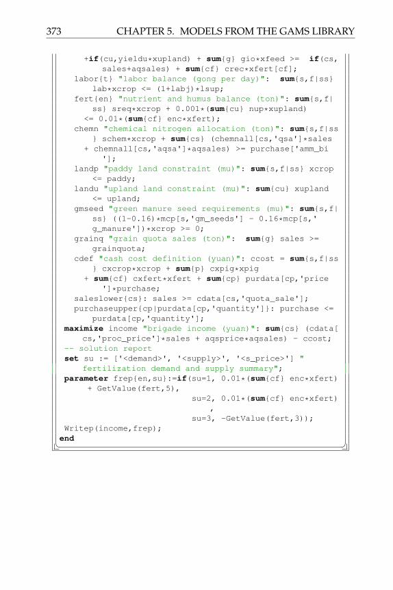
373 CHAPTER 5. MODELS FROM THE GAMS LIBRARY

+if(cu,yieldu*xupland) + sum{g} gio*xfeed >= if(cs,sales+aqsales) + sum{cf} crec*xfert[cf];

labor{t} "labor balance (gong per day)": sum{s,f|ss}lab*xcrop <= (1+labj)*lsup;

fert{en} "nutrient and humus balance (ton)": sum{s,f|ss} sreq*xcrop + 0.001*(sum{cu} nup*xupland)

<= 0.01*(sum{cf} enc*xfert);chemn "chemical nitrogen allocation (ton)": sum{s,f|ss

} schem*xcrop + sum{cs} (chemnall[cs,'qsa']*sales+ chemnall[cs,'aqsa']*aqsales) >= purchase['amm_bi

'];landp "paddy land constraint (mu)": sum{s,f|ss} xcrop

<= paddy;landu "upland land constraint (mu)": sum{cu} xupland

<= upland;gmseed "green manure seed requirements (mu)": sum{s,f|

ss} ((1-0.16)*mcp[s,'gm_seeds'] - 0.16*mcp[s,'g_manure'])*xcrop >= 0;

grainq "grain quota sales (ton)": sum{g} sales >=grainquota;

cdef "cash cost definition (yuan)": ccost = sum{s,f|ss} cxcrop*xcrop + sum{p} cxpig*xpig

+ sum{cf} cxfert*xfert + sum{cp} purdata[cp,'price']*purchase;

saleslower{cs}: sales >= cdata[cs,'quota_sale'];purchaseupper{cp|purdata[cp,'quantity']}: purchase <=

purdata[cp,'quantity'];maximize income "brigade income (yuan)": sum{cs} (cdata[

cs,'proc_price']*sales + aqsprice*aqsales) - ccost;-- solution reportset su := ['<demand>', '<supply>', '<s_price>'] "

fertilization demand and supply summary";parameter frep{en,su}:=if(su=1, 0.01*(sum{cf} enc*xfert)

+ GetValue(fert,5),su=2, 0.01*(sum{cf} enc*xfert)

,su=3, -GetValue(fert,3));

Writep(income,frep);end� �

CHAPTER 5. MODELS FROM THE GAMS LIBRARY 374

5.11. Financial Optimization: Financial Engineering(cmo)

Problem: Collateralized Mortgage Obligations (CMO) are used to restructurethe cashflows from underlying mortgage collateral into a set of high qualitybonds with different maturities. In the following mixed-integer programmingis used to restructure a mortgage pool into six normal tranches and on zerotranch. The model is written in a general form to allow experimentation withdifferent periodicity. The following version is annual.

This model is from the GAMS model library (GAMS SEQ=114). See also [7]

Modeling Steps

Listing 5.11: The Complete Model in LPL [15]� �model CMO "Financial Optimization: Financial Engineering"

;seti,j "tranches" := [ n1 n2 n3 n4 n5 n6 , m ];n{i} "normal tranches" := [ n1 n2 n3 n4 n5 n6 ];m{i} "m tranches" := [m];tp "time periods" := [ 0 1 2 3 4 5 6 7 8 9 10 ];ts{tp} "settlement date" := [ 0 ];t{tp} "payment periods" := [ 1 2 3 4 5 6 7 8 9 10 ];tl{tp} "last payment" := [ 10 ];

/* note: all rates are monthly rates x 12. Foraggregation we need to compute equivalent rates.(1+r/12)**12 == (1+rd)**d */

parametercg "collateral annual gross coupon" := 0.10;nom "nominal value of collateral" := 100;s "servicing rate" := 0.005;psa "pricing speed" := 115;d "periodicity" := 1;tmax "term to maturity of collateral" := #t;age "age of the collateral in years" := (360 -

tmax*12/d)/12;minn "minimum number of normal tranches" := 3;minm "minimum number of m tranches" := 1;--tranches datatrcoupon{i}:= [0.085 0.085 0.085 0.0875 0.0875

0.0875 /*0.0875 0.0875*/ 0.0995];tryield{i} := [0.099 0.0999 0.0999 0.1006 0.1009

0.1017 /*0.1018 0.1025*/ 0.105];trlowWal{n}:= [1.00 2.00 3.00 4.00 5.00 7.00 /*10.00

15.00*/];

375 CHAPTER 5. MODELS FROM THE GAMS LIBRARY

trupWal{n} := [1.24 2.44 3.44 4.44 5.65 7.94 /*10.9420.00*/];

tryr := 0.1285;rev{tp} "reverse order addresses" := #tp-2*tp + 1;cd "periodic gross coupon" := (1+cg/12)^(12/d

)-1;sd "periodic servicing rate" := (1+s/12)^(12/d

)-1;po{tp} "outstanding collateral principal at zero

prepayment" := nom*(1-1/(1+cd)^(tmax+1-tp))/(1-1/(1+cd)^tmax);

a "zero prepayment annuity" := nom*cd/(1-1/(1+cd)^tmax);

b{tp} "prepayment rate" := if(tp>1, 0.06*psa/100*Min((tp+age*d)/(d*2.5) , 1));

coupon{i} "periodic coupon by tranche" := (1+trcoupon/12)^(12/d)-1;

yield{i} "periodic yield by tranche" := (1+tryield/12)^(12/d)-1;

yr "periodic residual yield" := (1+tryr/12)^(12/d)-1;

cmax "maximum cmo coupon" := max{i} coupon;wallo{i} "lower weighted average life in periodicity

" := trlowWal*d;walup{i} "upper weighted average life in periodicity

" := trupWal*d;bv{tp} "temporary factor for bvf calculation";;

bv[#tp]:=0, {tp} (bv[tp+rev-1]:=(bv[tp+rev]+a-sd*po[tp+rev-1])/(1+cmax));

parameterbvf{tp} "bond value factor" := if(po,Min(bv/po,1),

#tp,1);pe{tp} "expected outstanding collateral principal"

;dum1 := pe[1]:=nom, for{tp|tp>1} (pe:=pe[tp-1]*(1-b)

^(1/d)*po/po[tp-1]);cflow{tp} "expected collateral payments" := if(tp

>1,(1+cd-sd)*pe[tp-1] - pe[tp]);prin{tp} "structuring principal payments from

collateral" := if(tp>1,pe[tp-1]*bvf[tp-1] - pe*bvf);

sump "sum of prin" := sum{tp} prin;psum{tp} "sum of principal payments on collateral

till tp";tpsum{tp} "sum of time principal payment products";dum2 := tpsum[1]:=0, psum[1]:=0, for{tp|tp>1} (psum:=

psum[tp-1]+prin, tpsum:=tpsum[tp-1]+(tp-1)*prin);walp{tp} "wal on principal payments from collateral"

:= if(tp>1,tpsum/psum);bign "big number":= sump*0.7;

CHAPTER 5. MODELS FROM THE GAMS LIBRARY 376

smalln "small number" := sump*0.03;setzpos{i,tp} "possible payment periods by tranche" :=

if(walp>walup and i within n,0,1);variablex{i,tp} "outstanding principal in each tranche";c{i,tp} "cashflow in each tranche";y{i,tp} "upper triangular structure";r{tp} "residual payments";pv{i} "def pv tranches";p{i,tp} [-1e18..1e18] "principal payments on tranches

";tpp{i} [-1e18..1e18] "product of time and principal

payment";pvres [-1e18..1e18] "def pv residuals";binary z{i,tp} "tranche utilization variable (1=usage

)";tin{i} "tranche in the structure";

constraintdefpv{i} "def pv tranches": pv = sum{t|zpos} 1/(1+

yield)^(t-1)*c;defpvres "def pv residuals": pvres = sum{t} 1/(1+yr)

^(t-1)*r;pdef{zpos[i,t]|t>1} "definition of principal payments

": p = x[i,t-1] - x;cdef{zpos[i,t]|t>1} "cashflow accounting": c =

coupon*x[i,t-1] + p;retiren1{t} "retirement of normal tranches": sum{n|

zpos} p = prin + sum{m} (x[m,tp-1]*coupon-c);retire{zpos[i,t]|i within n} "retirement of tranches"

: p <= cflow*z;retirem{m,t} "retirement of m tranche": c <= cflow*z

;retirem1{m,t} "retirement of m tranche": p <= prin*z;cbal{t} "cashflow balance": sum{i|zpos} c + r =

cflow;tppdef{n} "definition of tpp": tpp = sum{t|zpos}

(t-1)*p;lowal{n} "lower bound on weighted average life":

wallo*(sum{ts} x) <= tpp;upwal{n} "upper bound on weighted average life":

walup*(sum{ts} x) >= tpp;seq1{t} "sequencing constraint 1": sum{i|zpos}

z = 1;seq2{zpos[i,t]|t>1} "sequencing constraint 2": y >= y

[i,t+1];ydef{zpos[i,t]|t>1} "definition of y": y = y[i-1,t] +

z;tindef1{i} "tranche in definition": sum{ts} x <=

tin*bign;

377 CHAPTER 5. MODELS FROM THE GAMS LIBRARY

tindef2{i} "tranche in definition": sum{ts} x >=tin*smalln;

ncon "constraint on number of tranches": sum{n} tin>= minn;

mcon "constraint on number of m tranches": sum{m} tin>= minm;

pLow{n,tp}: p>=0;xfx1{i,tl}: x=0;xfx2{i,t|~zpos[i,t+1]}: x=0;zfx1{i,tp|~zpos}: z=0;zfx2{m,tp|~(sum{n} zpos)}: z=1;

maximize proceeds: sum{i} pv + pvres;Writep(proceeds,z,x,c,r);

end� �

CHAPTER 5. MODELS FROM THE GAMS LIBRARY 378

5.12. Peacefully Coexisting Armies of Queens (coex)

Problem: Two armies of queens (balck and white) peacefully coexist on achessboard when they are placed on the board in such a way that no twoqueens from opposing armies can attack each other. The problem is to findthe maximum two equal-sized armies.

This model is from the GAMS model library (GAMS SEQ=219). See also [2].

Modeling Steps

Listing 5.12: The Complete Model in LPL [15]� �model COEX "Peacefully Coexisting Armies of Queens";

set i ,j,ii "size of chess board" := [ 1..8 ];m{i,j,ii,jj in i} "shared positions on the board" :=

(i=ii) or j=jj or Abs(i-ii)=Abs(j-jj);binary variable b{i,j} "square occupied by a black

queen";w{i,j} "square occupied by a white queen";

variable tot "total queens in each army";constrainteq1{m[i,j,ii,jj]} "keeps armies at peace": b[i,j] + w

[ii,jj] <= 1;eq2 "add up all the black queens": tot = sum{i,j} b;eq3 "add up all the white queens": tot = sum{i,j} w;

maximize obj: tot;end� �

Solution:

opt: solution reported in OPTIMA

b.fx('6','2') = 1;b.fx('7','2') = 1;b.fx('8','2') = 1;b.fx('7','1') = 1;b.fx('8','1') = 1;b.fx('7','6') = 1;b.fx('8','6') = 1;b.fx('7','7') = 1;b.fx('8','7') = 1;

379 CHAPTER 5. MODELS FROM THE GAMS LIBRARY

5.13. Peacefully Coexisting Armies of Queens -tight (coexx)

Problem: We have set the size of the board to 5 in order to find solutionsquickly. In addition we fix the position of one queen. Two armies of queens(balck and white) peacefully coexist on a chessboard when they are placed onthe board in such a way that no two queens from opposing armies can attackeach other. The problem is to find the maximum two equal-sized armies.

This model is from the GAMS model library (GAMS SEQ=218). See also [2].

Modeling Steps

Listing 5.13: The Complete Model in LPL [15]� �model COEXX "Peacefully Coexisting Armies of Queens -

tight";set i ,j "size of chess board" := [1..8];

s "diagonal offset" :=[1..13]; --2i-3 diagonalsparameter sh{s} "shift values for diagonals" :=s-#i+1;rev{s,i} "reverse shift order" := #i+1-2*i+ sh;

binary variable xw{i,j} "has a white queen";xb{i,j} "has a black queen";wa{i} "white in row i";wb{i} "white in column j";wc{s} "white in diagonal s";wd{s} "white in backward diagonal s";

variable tot;constraintaw{i,j} "white in row i": wa[i] >= xw;bw{j,i} "white in column j": wb[j] >= xw[i,j];cw{s,i} "white in diagonal s": wc[s] >= xw[i,i+sh];dw{s,i} "white in backward diagonal s": wd[s] >= xw[i

,i+rev];ab{i,j} "black in row i": 1-wa[i] >= xb;bb{j,i} "black in column j": 1-wb[j] >= xb[i,j];cb{s,i} "black in diagonal s": 1-wc[s] >= xb[i,i+sh];db{s,i} "black in backward diagonal s": 1-wd[s] >= xb

[i,i+rev];eb "total black": tot = sum{i,j} xb;ew "total white": tot = sum{i,j} xw;fx11: xb[1,1] = 1; --fix one position in the NW

cornermaximize obj: tot;Writep(tot);

end� �

CHAPTER 5. MODELS FROM THE GAMS LIBRARY 380

5.14. Alcuin’s River Crossing (cross)

Problem: A farmer carrying a bushel of corn and accompanied by a goose anda wolf came to a river. He found a boat capable of transporting himself plusone of his possessions - corn, goose, or wolf - but no more. Now, he couldn’tleave the corn alone with the goose, nor the goose alone with the wolf, elseone would consume the other. Nevertheless, he succeeded in getting himselfand his goods across the river safely.

This model is from the GAMS model library (GAMS SEQ=191) (Contributedby Soren Nielsen, Institute for Mathematical Sciences University of Copen-hagen). See also [1].

Modeling Steps

Listing 5.14: The Complete Model in LPL [15]� �model CROSS "Alcuin's River Crossing";

set i "items" := [goose, wolf, corn];t "time" := [1..10];

parameter dir{t} "crossing - near to far is +1 - farto near -1" := -1^(t-1);

variablecross{i,t} "crossing the river";done{t} "all items in far side";binary y{i,t} "1 iff the item is on the far side at

time t";constraintDefCross{i,t|t>1} "crossing": y = y[i,t-1] + dir[t

-1]*cross[i,t-1];DefDone{i,t} "everything on far side": done <= y;limCross{t|t>1}: sum{i} cross[i,t-1] <= 1;EatNone1{t}: dir*(y['goose',t] + y['wolf',t] - 1) <=

done;EatNone2{t}: dir*(y['goose',t] + y['corn',t] - 1) <=

done;yFx{i}: y[i,1] = 0;

maximize nocross "number of non crossing periods": sum{t} done;

Writep(nocross,y,cross);end� �

381 CHAPTER 5. MODELS FROM THE GAMS LIBRARY

5.15. 3-dimensional Noughts and Crosses (cube)

Problem: White and black balls are to be arranged in a cube one to a cell insuch a way as to minimize the number of lines with balls of equal color. Forthis example the length of the cube is three. a total of 49 lines exist in a cube of3x3x3. 27 lines by changing only one coordinate, 18 diagonals within a plane,and 4 diagonals going across planes. (see Will16.lpl)

This model is from the GAMS model library (GAMS SEQ=42). See also [28]and te model WILL16.

Modeling Steps

Listing 5.15: The Complete Model in LPL [15]� �model CUBE "3-dimensional Noughts and Crosses";set s,sp,spp "domain for line" := [a b c incr decr];

x,y,z{s} "coordinate labels" := [ a, b, c ];d,dp{s} "directions" := [ incr, decr ];b "bounds" := [ low, high ];

ld{s,sp,spp} "line definition" :=(s='incr' and sp within x and spp within x ors within x and sp='incr' and spp within x ors within x and sp within x and spp='incr' ors='incr' and sp within d and spp within x ors within x and sp='incr' and spp within d ors within d and sp within x and spp='incr' ors='incr' and sp within d and spp within d);

parameterls{b} "sign for line definitions" :=/low 1 high -1/;lr{b} "rhs for line definitions" :=/low 2 high -1/;df{x,s} "line definition function" := if(s='decr',1+#

x-2*x, s='incr',0, s-x);variableline{s,sp,spp} "line identification";binary core{x,y,z} "placement of balls (white 0

black 1)";constraintnbb "total number of balls definition": sum{x,y,z}

core = Floor(#x^3/2);ldef{ld[s,sp,spp],b} "line definitions": ls*(sum{x}

core[x+df[x,s],x+df[x,sp],x+df[x,spp]]) <= line+lr;

minimize num "number of lines of equal color": sum{ld[s,sp,spp]} line;

Writep(num,core,line);end� �

CHAPTER 5. MODELS FROM THE GAMS LIBRARY 382

5.16. Simple Farm Level Model (demo1)

Problem: This is the first in a series of single farm models . This simplestversion has only 7 principal crops and 2 basic inputs, land and labor, whichare specified on a monthly basis.

This model is from the GAMS model library (GAMS SEQ=91). See also [19]

Modeling Steps

Listing 5.16: The Complete Model in LPL [15]� �model DEMO1 "Simple Farm Level Model";

set c "crops" := [ wheat, clover, beans, onions, cotton, maize, tomato ];t "period" := [ jan, feb, mar, apr, may, jun, jul,

aug, sep, oct, nov, dec ];parameter landreq{t,c} "months of land occupation by

crop (hectares)" := [1.0 1.0 1.0 1.0 . . .1.0 1.0 1.0 1.0 . . .1.0 0.5 1.0 1.0 0.5 . .1.0 . 1.0 1.0 1.0 . .1.0 . . 0.25 1.0 0.25 .. . . . 1.0 1.0 .. . . . 1.0 1.0 0.75. . . . 1.0 1.0 1.0. . . . 1.0 1.0 1.0. . . . 1.0 .5 1.0

0.5 0.25 0.25 0.5 0.75 . 0.751.0 1.0 1.0 1.0 . . . ];

laborreq{t,c} "crop labor requirements (man days perhectare)" := [1.72 4.5 0.75 5.16 . . .0.5 1.0 0.75 5.0 . . .1.0 8.0 0.75 5.0 5.0 . .1.0 . 16. 19.58 5.0 . .

17.16 . . 2.42 9.0 4.3 .2.34 . . . 2.0 5.04 .. . . . 1.5 7.16 17.0. . . . 2.0 7.97 15.0. . . . 1.0 4.41 12.0. . . . 26.0 1.12 7.0

2.43 2.5 7.5 11.16 12.0 . 6.01.35 7.5 0.75 4.68 . . . ];

yield{c} "crop yield (tons per hectare)" := /wheat 1.5, clover 6.5, beans 1, onions 3

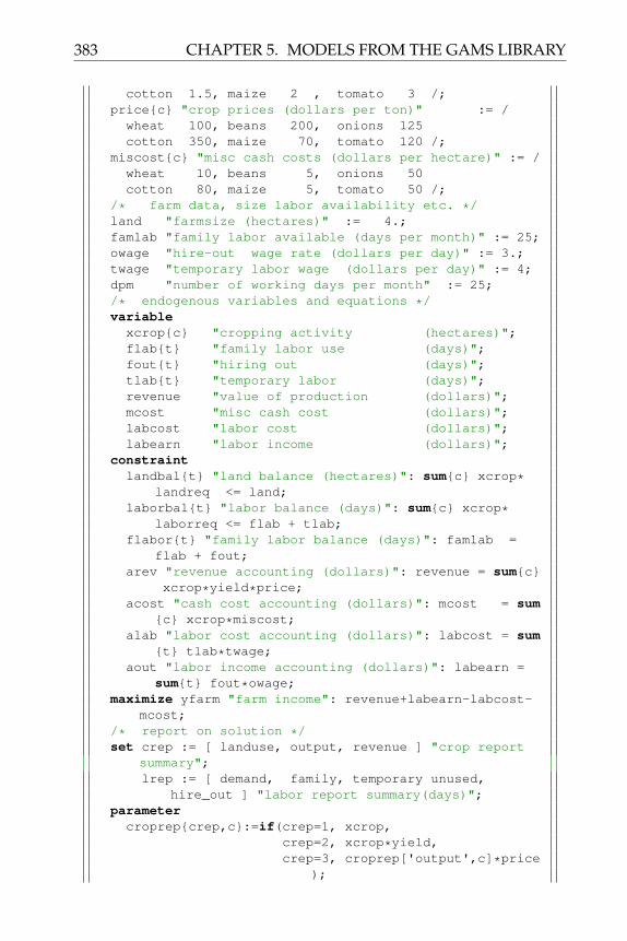
383 CHAPTER 5. MODELS FROM THE GAMS LIBRARY

cotton 1.5, maize 2 , tomato 3 /;price{c} "crop prices (dollars per ton)" := /wheat 100, beans 200, onions 125cotton 350, maize 70, tomato 120 /;

miscost{c} "misc cash costs (dollars per hectare)" := /wheat 10, beans 5, onions 50cotton 80, maize 5, tomato 50 /;

/* farm data, size labor availability etc. */land "farmsize (hectares)" := 4.;famlab "family labor available (days per month)" := 25;owage "hire-out wage rate (dollars per day)" := 3.;twage "temporary labor wage (dollars per day)" := 4;dpm "number of working days per month" := 25;/* endogenous variables and equations */variablexcrop{c} "cropping activity (hectares)";flab{t} "family labor use (days)";fout{t} "hiring out (days)";tlab{t} "temporary labor (days)";revenue "value of production (dollars)";mcost "misc cash cost (dollars)";labcost "labor cost (dollars)";labearn "labor income (dollars)";

constraintlandbal{t} "land balance (hectares)": sum{c} xcrop*

landreq <= land;laborbal{t} "labor balance (days)": sum{c} xcrop*

laborreq <= flab + tlab;flabor{t} "family labor balance (days)": famlab =

flab + fout;arev "revenue accounting (dollars)": revenue = sum{c}

xcrop*yield*price;acost "cash cost accounting (dollars)": mcost = sum

{c} xcrop*miscost;alab "labor cost accounting (dollars)": labcost = sum

{t} tlab*twage;aout "labor income accounting (dollars)": labearn =

sum{t} fout*owage;maximize yfarm "farm income": revenue+labearn-labcost-

mcost;/* report on solution */set crep := [ landuse, output, revenue ] "crop report

summary";lrep := [ demand, family, temporary unused,

hire_out ] "labor report summary(days)";parametercroprep{crep,c}:=if(crep=1, xcrop,

crep=2, xcrop*yield,crep=3, croprep['output',c]*price

);

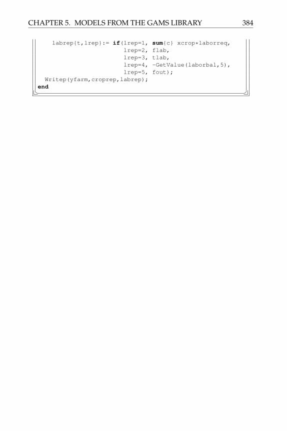
CHAPTER 5. MODELS FROM THE GAMS LIBRARY 384

labrep{t,lrep}:= if(lrep=1, sum{c} xcrop*laborreq,lrep=2, flab,lrep=3, tlab,lrep=4, -GetValue(laborbal,5),lrep=5, fout);

Writep(yfarm,croprep,labrep);end� �

385 CHAPTER 5. MODELS FROM THE GAMS LIBRARY

5.17. Non-transitive Dice Design (dice)

Problem: Probabilistic dice - an example of a non-transitive relation. We wantto design a set of dice with an integer number on each face such that on av-erage dice1 beats dice2, and dice2 on average beats dice3 etc, but diceN hasto beat dice1. MIP codes behave very erratic on such a problem and slightreformulations can result in dramatic changes in performance. Also note theface value will be integers automatically.

This model is from the GAMS library (GAMS SEQ=176). See [4].

Modeling Steps

Listing 5.17: The Complete Model in LPL [15]� �model DICE "Non-transitive Dice Design";

set f ,fp "faces on a dice" := [1..6];dice ,d "number of dice" := [dice1 dice2 dice3];

parameterflo "lowest face value" := 1;fup "highest face value" := #dice*#f;wn "wins needed - possible bound" := Floor(0.5*#f

^2)+1;variablewnx "number of wins";fval{d,f} [flo..fup] "value of dice - will be

integer";binary comp{d,f,fp} "one if f beats fp";

constraintffx: fval['dice1','1'] = flo;equ1{d} "count the wins": sum{f,fp} comp = wnx;eq3{d,f,fp} "definition of non-transitive relation":

fval+(fup-flo)*(1-comp) >= fval[d%#d+1,fp]+1;eq4{d,f|f<#f} "different face values for a single

dice": fval+1 <= fval[d,f+1];maximize obj: wnx;Writep(wnx);

end� �

CHAPTER 5. MODELS FROM THE GAMS LIBRARY 386

5.18. Stigler’s Nutrition model (diet1)

Problem: This model determines a least cost diet which meets the daily al-lowances of nutrients for a moderately active man weighing 154 lbs.

This model is from the GAMS library (GAMS SEQ=7) and from [8], Chap 27.1.

Modeling Steps

Listing 5.18: The Complete Model in LPL [15]� �model DIET "Stigler's Nutrition model";

setn "nutrients" := [ calorie /*thousands*/, protein /*

grams*/ , calcium /*grams*/, iron /*milligrams*/vitamin_a /*thousand ius*/, vitamin_b1 /*milligrams*/, vitamin_b2 /*milligrams*/, niacin/*milligrams*/, vitamin_c /*milligrams*/ ];

f "foods" := [ wheat, cornmeal, cannedmilk, margarine, cheese, peanut_b, lard liver, porkroast, salmon, greenbeans, cabbage, onions, potatoes spinach,sweet_pot, peaches, prunes, limabeans, navybeans];

parameter b{n} "required daily allowances of nutrients":=

/ calorie 3, protein 70, calcium 0.8, iron 12vitamin_a 5, vitamin_b1 1.8, vitamin_b2 2.7,niacin 18, vitamin_c 75 /;

a{f,n} "nutritive value of foods (per dollar spent)":= [

/*(1000) (g) (g) (mg)(1000iu)(mg) (mg) (mg) (mg)

*/44.7 1411 2.0 365 . 55.4 33.3 441 .36 897 1.7 99 30.9 17.4 7.9 106 .8.4 422 15.1 9 26 3 23.5 11 6020.6 17 0.6 6 55.8 0.2 . . .7.4 448 16.4 19 28.1 0.8 10.3 4 .15.7 661 1 48 . 9.6 8.1 471 .41.7 . . . 0.2 . 0.5 5 .2.2 333 0.2 139 169.2 6.4 50.8 316 5254.4 249 0.3 37 . 18.2 3.6 79 .5.8 705 6.8 45 3.5 1 4.9 209 .2.4 138 3.7 80 69 4.3 5.8 37 8622.6 125 4 36 7.2 9 4.5 26 53695.8 166 3.8 59 16.6 4.7 5.9 21 118414.3 336 1.8 118 6.7 29.4 7.1 198 25221.1 106 . 138 918.4 5.7 13.8 33 2755

387 CHAPTER 5. MODELS FROM THE GAMS LIBRARY

9.6 138 2.7 54 290.7 8.4 5.4 83 19128.5 87 1.7 173 86.8 1.2 4.3 55 5712.8 99 2.5 154 85.7 3.9 4.3 65 25717.4 1055 3.7 459 5.1 26.9 38.2 93 .26.9 1691 11.4 792 . 38.4 24.6 217 .

];variable x{f} "dollars of food f to be purchased daily

(dollars)";constraint nb{n} "nutrient balance (units)": sum{f} (a

[f,n]*x) >= b;minimize cost "total food bill (dollars)": sum{f} x;Writep(cost,x);

end� �

CHAPTER 5. MODELS FROM THE GAMS LIBRARY 388

5.19. Fertilizer Production (egypt)

Problem: This is a one-period model of the Egyptian fertilizer industry devel-oped at the World Bank. (for a GAMS representation see also: BISSCHOP J.,MEERAUS A., On the Development of a General Algebraic Modeling Systemin a Strategic Planning Environment. Development Research Department,Mathematical Programming Study 20, pp.1-29, 1982. and CHOKSI A.M.,MEERAUS A., STOUTJESDIJK, The Planning of Investment Programs in theFertilizer Industry, Johns Hopkins University Press, Batimore, 1980.

Cited also in: FOURER R., A Modeling Language for Mathematical Program-ming, 1987

A model formulation is as follows:

The Model

function Egyptset Center (Ce) , P (i, j) “Plants”set Port (Po) , Region (R) , Units (Un) , Process (Pr) , Nutr (N) ,

Commod (C, c) , cRaw (r) , cInter , cShip (s) , cFinal (f)param exch := 0.4param utilPct := 0.85set pExceptP,Prparam cf75R,cFinal , fncFinal,N , roadR,Ce , railHalfP,P , impdBargP

, impdRoadP , ioC,Pr , utilUn,Pr , pImpC , pRcRaw , pPrP,cRaw ,dcapP,Un , raili,j := if(railHalfi,j, railHalfi,j, railHalfj,i)

param tranFinalP,R := 0.5+ 0.0144 · roadR,PwithinCe

param tranImportR,Po := 0.5+ 0.0144 · roadR,PowithinCe

param tranInteri,j := 3.5+ 0.03 · raili,jparam tranRawP := if(impdBargP, 1+0.003·impdBargP)+if(impdRoadP, 0.5+

0.144 · impdRoadP)param pDomP,cRaw := if(pRcRaw, pRcRaw, pPrP,cRaw)param icapUn,P := 0.33 · dcapP,Un

set mPosP,Un := icapUn,P > 0set pCapP,Pr := ∀Un|utilUn,Pr>0 mPosP,Un

set pPosP,Pr := pCapP,Pr ∧ ¬pExceptP,Prset cpPosC,P :=

∑Pr|pPosP,Pr

ioC,Pr > 0

set ccPosC,P :=∑

Pr|pPosP,PrioC,Pr < 0

set cPosC,P := cpPosC,P ∨ ccPosC,P

var ZP,Pr|pPosP,Pr, XfcFinal,P,R|cpPoscFinalwithinC,P

, Xis,i,j|cpPosswithinC,i∧ccPosswithinC,j

, VfcFinal,R,Po , VrcRaw,P|ccPoscRawwithinC,P, UcRaw,P|ccPoscRawwithinC,P∧pDomP,cRaw>0

, Psip , Psil , Psii

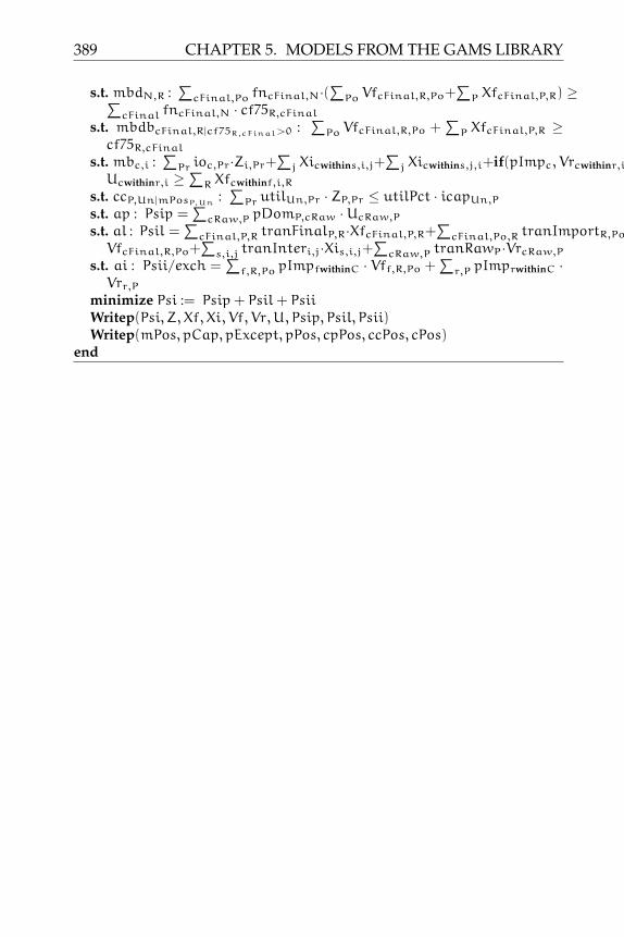
389 CHAPTER 5. MODELS FROM THE GAMS LIBRARY

s.t. mbdN,R :∑

cFinal,Po fncFinal,N·(∑

Po VfcFinal,R,Po+∑

P XfcFinal,P,R) ≥∑cFinal fncFinal,N · cf75R,cFinal

s.t. mbdbcFinal,R|cf75R,cFinal>0 :∑

Po VfcFinal,R,Po +∑

P XfcFinal,P,R ≥cf75R,cFinal

s.t. mbc,i :∑

Pr ioc,Pr·Zi,Pr+∑

j Xicwithins,i,j+∑

j Xicwithins,j,i+if(pImpc, Vrcwithinr,i)+Ucwithinr,i ≥

∑R Xfcwithinf,i,R

s.t. ccP,Un|mPosP,Un:∑

Pr utilUn,Pr · ZP,Pr ≤ utilPct · icapUn,P

s.t. ap : Psip =∑

cRaw,P pDomP,cRaw ·UcRaw,P

s.t. al : Psil =∑

cFinal,P,R tranFinalP,R·XfcFinal,P,R+∑

cFinal,Po,R tranImportR,Po·VfcFinal,R,Po+

∑s,i,j tranInteri,j·Xis,i,j+

∑cRaw,P tranRawP·VrcRaw,P

s.t. ai : Psii/exch =∑

f,R,Po pImpfwithinC · Vff,R,Po +∑

r,P pImprwithinC ·Vrr,P

minimize Psi := Psip+ Psil+ PsiiWritep(Psi, Z, Xf, Xi, Vf, Vr,U, Psip, Psil, Psii)Writep(mPos, pCap, pExcept, pPos, cpPos, ccPos, cPos)

end

CHAPTER 5. MODELS FROM THE GAMS LIBRARY 390

5.20. House Plan Design (house)

Problem: This problem designs the size of an L shaped house meeting limita-tions imposed by city codes and aesthetic considerations.

This model is from the GAMS library (GAMS SEQ=99) and from Borland,Eureka: The Solver. Tech. rep., Borland International, 1987.

Modeling Steps

Listing 5.19: The Complete Model in LPL [15]� �model HOUSE "House Plan Design";

variablex := 30 "width of front wing (ft)";y "length of front wing (ft)";z "length of second story (ft)";b [40..68] := 68 "total house width (ft)";a "length of back wing (ft)";l [56..100] "total house length (ft)";a1 [0..3000] "area of first floor (sq ft)";a2 "area of the second floor (sq ft)";

constraintdefa1 "definition of first floor area (sq ft)": a1 =

x*y+a*b;defa2 "definition of second floor area (sq ft)": a2 =

x*z;maxw "front wing maximum width (ft)": b/3<=x<=b/2;minp "minimum pool area (sq ft)": y*(b-x) >= 1500;defl "definition of total house length(ft)": l=y+a;balk "balkoney size restriction (ft)": z = a+y/2;prop "wing proportionality (ft)": a >= y/2;

maximize obj "total area of the house (sq ft)": a1+a2;Writep(obj);Draw.Scale(7,7);Draw.Line(0,0,b,0); Draw.Text('b='&b,b/3,1);Draw.Line(0,0,0,l); Draw.Text('l='&l,1,l/2);Draw.Line(b,0,b,a); Draw.Text('a='&a,b,a/2);Draw.Line(0,l,x,l); Draw.Text('x='&x,x/3,l-2);Draw.Line(x,l-y,x,l);Draw.Text('y='&y,x/2,a+(l-y)/1.5);Draw.Line(x,l-y,b,a);Draw.Line(0,l-y/2,x,l-y/2); Draw.Text('Balcony',2,l-y

/2+2);Draw.Text('Swimming Pool',x+2,l-y/2+2);

end� �

391 CHAPTER 5. MODELS FROM THE GAMS LIBRARY

5.21. Tanglewood Chair Manufacturing (tangle)Model from : MATURANA S. V., Survey and Analysis of LINGO, Mgt 298DCourse Project; John E. Anderson Graduate School of Management, Univer-sity of California, Los Angeles, CA 90024, p.17f

Problem: The Tanglewood Chair Manu. Co. has four plants located aroundthe country. The fabrication data are the following:

Plant Cost per chair Max production Min productionP1 5 500 0P2 7 750 400P3 3 1000 500P4 4 250 250

The wood required to make each chair is twenty pounds and is obtained fromtwo suppliers. The company purchase of at least 8 tons of wood per monthfrom each supplier. The cost of wood is 0.10/lb from supplier 1 and 0.075/lbfrom supplier 2. The shipping cost in dollar per pound of wood from eachsupplier to each plant is shown below:

P1 P2 P3 P4sup1 0.01 0.02 0.04 0.04sup2 0.04 0.03 0.02 0.02

The chairs are sold in New York, Houston, San Francisco and Chicago. Thetransportation costs are shown below:

NY H SF CP1 1 1 2 0P2 3 6 7 3P3 3 1 5 3P4 8 2 1 4

Following data are also available:

City Selling price maximum demand minimum demandNY 20 2000 500H 15 400 100SF 20 1500 500C 18 1500 500

Where should each plant buy its raw materials? How many chairs should bemade at each plant? How many chairs should be sold at each city? Whereshould each plant ship its product?

CHAPTER 5. MODELS FROM THE GAMS LIBRARY 392

5.22. A Travel Optimization Problem (travel)

SCICON Ltd. (or Spectrum, 1984, 6, p.125-130References

393 CHAPTER 5. MODELS FROM THE GAMS LIBRARY

5.23. A Transportation Problem (trnsport)

Problem: This problem finds a least cost shipping schedule that meets re-quirements at markets and supplies at factories. From Gams model librarySEQ=1. [8], chap 3.3, and [25], chap 2.

Listing 5.20: The Complete Model in LPL [15]� �model trnsport "A Transportation Problem";

seti "canning plants" := [ seattle, 'san-diego' ];j "markets" := [ 'new-york', chicago, topeka ];

parametera{i} "capacity of plant i in cases" :=/ seattle 350, 'san-diego' 600 /;

b{j} "demand at market j in cases" :=/ 'new-york' 325, chicago 300, topeka 275 /;

d{i,j} "distance in thousands of miles" := [2.5 1.7 1.82.5 1.8 1.4 ];

f "freight in dollars per case per thousand miles" :=90;

c{i,j} := f*d/1000 "transport cost in thousands ofdollars per case";

variable x{i,j} "shipment quantities in cases";constraintsupply{i}: sum{j} x <= a "observe supply limit at

plant i";demand{j}: sum{i} x >= b "satisfy demand at market j

";minimize cost: sum{i,j} c*x "total transportation costs

in thousands of dollars";Writep(cost,x);

end� �

CHAPTER 6

MISCELLANEOUS

6.1. A simple blending problem (alloy)

Problem: A small blending problem

Listing 6.1: The Complete Model in LPL [15]� �model ALLOYING "A simple blending problem";

setmetals,m := [ A,B,C1,C2,D ];ores, o := [ ore1 ore2 ore3 ore4 ore5 ore6 ];

parameterbound{o} "availability of ore"

:= [1000 3000 2000 800 2600 1700];boundu{o} "availability of ore"

:=0;price {o} := [25 10 20 18 22 12 ];purity{o} := [ 0.8 0.4 0.7 0.6 0.7 0.4];alloy{m} := [ 0.18 -0.30 -0.40 0.60 0.02];obtain{o,m} := [

0.20 -0.20 -0.40 0.40 0.000.15 -0.00 -0.20 0.20 0.050.00 -0.40 -0.30 0.30 0.000.10 -0.20 -0.30 0.30 0.000.10 -0.25 -0.25 0.25 0.100.05 -0.08 -0.17 0.17 0.10];

quantity,Q := 3000;variable AMOUNT,X{o} [boundu..bound];constraintquareq: sum{o} purity*X = Q "Quantity to produce";metreq{m}: sum{o}(alloy*purity-obtain)*X >= 0 "Metal

requirements";minimize cost: sum{o} price*X "Minimize costs";Writep(cost,X);

end� �395

CHAPTER 6. MISCELLANEOUS 396

6.2. Assign Consulters (assign1)

Problem: A consulter company plans to distibute its consulter with differentknowledge into the different projects over the periods. Each project needsvarious knowledge in the different time periods.

Modeling Steps

Listing 6.2: The Complete Model in LPL [15]� �model assign1 "Assign Consulters";

set c "Consulters";k "knowledge";t "time periods";p "projects";CK{c,k} "c has the knowledge k";PK{p,k,t} "project uses knowledge in time";

parameter level{c};binary variable x{c,p,t};constraintR{c,t}: sum{p} x <=1 "In each period, a consulter can

only be with one project";S{p,t,k|PK}: sum{c|CK} x>=1 "The project must be

adequatly accompanied";minimize obj: sum{c,p,t} level*x "minimize the pool of

consulter";model data;c := [1..5];k := [1..3];t := [1..20];p := [1..3];CK{c,k} := [1 1, 1 2, 2 2, 2 3, 3 3, 4 1, 5 2, 5 1];PK{p,k,t} := if(Rnd(0,1)>0.2,Trunc(Rnd(0,2)),0);level{c} := [1 2 3 4 5];

endmodel output;Writep(PK,x);

endend� �

397 CHAPTER 6. MISCELLANEOUS

6.3. Agriculture Production (crop)

Problem: see Katz S. (IBM Systems Journal 19:4,1980, p.505-520, Appendix B)

Listing 6.3: The Complete Model in LPL [15]� �model CROP "Agriculture Production";

setMonth,m := [ May June July ];Crop,c := [ Cotton Onion Pear Avoccado ];Field,f := [ Cotton Onion ];

parameterWaterBND{m} := [200000 260000 270000];Labor{c} := [2.9 2.7 1.0 1.5];Profit{c} := [6453 6110 4814 8813];Ceils{c}:= [2000 250 500 800];Land:=2700; FieldLand:=1850; LaborTot:=5850;Water{c,m}:=[65 80 90 . 60 . . 53 64 . 75 85];

variable CropVar{c} [0..Ceils];constraintr1: sum{c} CropVar <= Land;r2: sum{f} CropVar[f within Crop] <= FieldLand;wat{m}: sum{c} Water*CropVar <= WaterBND;r3: sum{c} Labor*CropVar <= LaborTot;

maximize prof: sum{c} Profit*CropVar;Writep(prof,CropVar);

end� �

CHAPTER 6. MISCELLANEOUS 398

6.4. Import and Export Goods (export)

Problem: A country has four industries: Steel, Automotive, Electronics andPlastics. There unit prices are: 500, 1500, 300 and 1200. The total availableManpower is 830,000 year-hours. No more than 650,000 units of Automotiveand 60,000 units of Plastic can be produced. Production of 1 unit of Steel re-quires 0.02 unit of Automotive, 0.01 units of Plastics, 250 currency units ofimported raw matrials and 0.5 manpower unit. Production of 1 unit of Au-tomotive reqires 0.8 unit of steel, 0.15 units of electronics 0.11 units of plastic,300 units of imported materials and 1 manpower unit. Production of 1 unitof Electronics reqires 0.01 unit of steel, 0.01 units of automotive, 0.05 units ofplastic half a man years of labor and 50 units of imported materials. Produc-tion of 1 unit of plastics requires .03 units of automotive production,

1. units of steel, 0.05 units of electronics, 2 man years of labor and

2. units of imported materials. The economic minister would like to max-imize the exceeding export value.

Schrage L.,LINDO, 1986, p.116f.";References

Listing 6.4: The Complete Model in LPL [15]� �model EXPORT "Import and Export Goods";

set i,j := [ steel automotive electronic plastics];parameter prices{i}:=[500 1500 300 1200];ImportCosts{i}:=[250 300 50 300];ManPowerUsed{i}:=[.5 1 .5 2];Limits{i}:=[. 650000 . 60000];ManPower := 830000;Inputs{i,j} :=

[. .8 .01 .2 , .02 . .01 .03 , . .15 . .05 , .01.11 .05 . ];

variable P{i} "PRODUCTION"; E{i} "EXPORTS";constraintA{i}: P = E + sum{j} Inputs[i,j]*P[j];B: sum{i} ManPowerUsed*P = ManPower;C{i|Limits}: P <= Limits;

maximize obj: sum{i} ( prices*E - ImportCosts*P );Writep(obj,P,E);

end� �

399 CHAPTER 6. MISCELLANEOUS

6.5. A Small Portfolio Model (lin193)Mode from SCHRAGE, Lindo , page 193.

Listing 6.5: The Complete Model in LPL [15]� �model LIN193 "A Small Portfolio Model";

variable x; y; z; budget; yield; xfrac; yfrac; zfrac;constraintR1: 6*x+2*y-z + budget-1.3*yield+xfrac >= 0;R2: 2*x+4*y-0.8*z + budget-1.2*yield+yfrac >= 0;R3: -x-0.8*y+2*z + budget-1.08*yield+zfrac >= 0;R4: x+y+z=1;R5: 1.3*x+1.2*y+1.08*z >= 1.12;R6: x <= 0.75;R7: y <= 0.75;R8: z <= 0.75;

minimize obj: x+y+z+budget+yield+xfrac+yfrac+zfrac;Writep(obj,x,y,z,budget,yield,xfrac,yfrac,zfrac);

end� �

CHAPTER 6. MISCELLANEOUS 400

6.6. Exposures in Media Vehicles (media)

Problem: An advertising agency plans to select the media mix that will max-imize the number of effective exposures subject to a set of constraints. Thereare three media vehicles A, B and C. Vehicle A gives 3,100 (in thousands) ef-fective exposures per issue , vehicle B gives 2,000, and vehicle C gives 2,400.The media planner has an advertising budget of $500,000, which cannot beexceeded. Vehicle A costs $15,000 per issue, vehicle B, $4,000, and vehicle C,$5,000. Furthermore, the media planner wants to spend at least $250,000 onvehicle A. Vehicle A puts out 52 issues a year, vehicle B, eight issues, and ve-hicle C, twelve issues. The media planner wants to buy at least one issue ofvehicle B and six issues of vehicle C.

Listing 6.6: The Complete Model in LPL [15]� �model MEDIA "Exposures in Media Vehicles";

set media := [A B C ];parameter ExposureCost{media} := [ 15000 4000 5000 ];Issues{media} := [ 3100 2000 2400 ];PutsOutPerYear{media} := [ 52 8 12 ];MinimalExposures{media} := [ . 1 6 ];Budget := 500000;MinimalBudgetForA := 250000;

variable NumberOfExposures{media} [MinimalExposures..PutsOutPerYear];

constraintr1: sum{media} ExposureCost*NumberOfExposures <=

Budget;r2: ExposureCost['A']*NumberOfExposures['A'] >=

MinimalBudgetForA;maximize number: sum{media} Issues*NumberOfExposures;Writep(number,NumberOfExposures);

end� �

401 CHAPTER 6. MISCELLANEOUS

6.7. Mexican Steel Industry (mexican)

Model from MATURANA S. V., Survey and Analysis of LINGO, Mgt 298DCourse Project; John E. Anderson Graduate School of Management, Univer-sity of California, Los Angeles, CA 90024, p.23f

Listing 6.7: The Complete Model in LPL [15]� �model Mexican "Mexican Steel Industry";set

plants := [AHMSA FUNDIDOR SICARTSA HYLSA HYLSAP];markets := [MexicoDF Monterey Guadalaj];cf := [STEEL];ci := [ SPONGE PIGIRON ];cr := [PELLETS COKE NATGAS ELECTRIC SCRAP];process :=[pigironp spongep steeloh steelel steelbof];produnit := [blastfrn ofenhrth bof directed elecarc];

parameterrd2{plants}:=[739 521 . 521 315];dd{markets}:=[55 30 15];rd3{markets}:=[428 521 300];pv{cf}:=[150]; pe{cf}:=[140]; eb{cf}:=[1];pd{cr}:=[18.7 52.17 14 24 105];

parameterDT := 5.209;rse := 40;k{produnit,plants} := [ 3.25 1.40 1.1 0 0

1.5 0.85 0 0 02.07 1.5 1.3 0 00 0 0 0.98 10 0 0 1.13 0.56 ];

rd1{plants,markets} :=[ 1204 218 1125, 1017 . 1030,

819 1305 704, 1017 . 1030,185 1085 760 ];

b{produnit,process} :=[ 1 0 0 0 0,0 0 1 0 0,0 0 0 0 1,0 1 0 0 0,0 0 0 1 0

];a1{cr,process} := [ -1.58 -1.38 0 0 0

-0.63 0 0 0 00 -0.57 0 0 00 0 0 -0.58 00 0 -0.33 0 -0.12 ];

a2{ci,process} := [ 1.00 0 -0.77 0 -0.950 1.00 0 -1.09 0 ];

a3{cf,process} := [ 0 0 1.0 1.0 1.0 ];variable

phipsi; philam; phipi; phieps;z{process,plants};

CHAPTER 6. MISCELLANEOUS 402

u{cr,plants};e{cf,plants};d{cf,markets};v{cf,markets};x{cf,plants,markets};

constraintr1{cf,markets}: d = DT*(1+rse/100)*dd/100;mbf{cf,plants}: sum{process} a3*z >= sum{markets} x +e;mbi{ci,plants}: sum{process} a2*z >= 0;mbr{cr,plants}: sum{process} a1*z + u >= 0;cc{produnit,plants}: sum{process} b*z <= k;mr{cf,markets}: sum{plants} x+v >= d;me{cf}: sum{plants} e <= eb;r2: phipsi = sum{cr,plants} pd*u;r3: philam = sum{cf,plants,markets} if(rd1 , (0.0084*

rd1+2.48)*x)+ sum{cf,plants} if(rd2,(0.0084*rd2+2.48)*e)+ sum{cf,markets} if(rd3,(0.0084*rd3+2.48)*v);

r4: phipi = sum{cf,markets} pv*v;r5: phieps = sum{cf,plants} pe*e;

minimize phi: phipsi + philam + phipi - phieps;Writep(phi);end� �

403 CHAPTER 6. MISCELLANEOUS

6.8. A Production Planning Model (omp)

Problem: An application of aggregate multiperiod production planning: Acompany has 5 products to manufacture on 5 machine types. How muchshould be manufactured, stored, and sold in each period over the next 6 peri-ods (6 months) in order to maximize the contribution. The production capac-ity on each machine is limited, as well as the sales. The prices of the productsare given. At the end of the six periods the company wants a stock of 50units of each product in its inventory. The inventory is empty at the begin-ning of the first period. The only costs are the inventory: each unit of eachproducts costs 0.5 (money-unit) in each period. (The model is from: O.M.P.Optimisation, an Application of the Model Generator to Aggregate Produc-tion Planning, A brochure of Beyers and Partners, pp. 3-11.)

Modeling Steps

The data of the problem are given as follows.

1. There are three sets: the time periods (t), the products (p), and the ma-chines (m).

2. The prices for each product is Pricep.

3. Timem,p is the time (in hours) that a machine m takes to manufactureone unit of product p.

4. Limitt,p is the upper limit of sales of a product p in period t.

5. Capacityt,m is the quantity of any product a machine m can manufac-ture in period t.

6. We introduce three variables: the quantity of products p that are manu-factured in period t: Manufp,t; the quantity sold of product p in periodt: Salesp,t, and the quantity stored of product p at the end of time pe-riod t: Stockp,t.

7. The inventory at the end of the last period must be 50:

Stockp,JUN = 50 forall Period p

8. The proction should not exceed the capacities of the machines:∑p

Timem,p ·Manufp,t ≤ Capacityt,m forall (m, t)

9. The product balance over the periods must hold:

Manufp,t + Stockp,t−1 = Stockp,t + Salesp,t forall (p, t)

CHAPTER 6. MISCELLANEOUS 404

10. The contribution (to be maximized) is:∑p,t

(Pricep · Salesp,t − 0.5 · Stockp,t)

Listing 6.8: The Complete Model in LPL [15]� �model OMP "A Production Planning Model";

sett := [ JAN FEB MAR APR MAY JUN ] "Time periods";p := [ Prod1 Prod2 Prod3 Prod4 Prod5 ] "Products";m := [ MACHA MACHB MACHC MACHD MACHE ] "machines";

parameterPrice{p} := [ 10 6 8 4 11 ];Time {m,p} "Production time unit of a product at a

machine" :=[ 0.5 0.7 . . 0.3

0.1 0.2 . 0.3 .0.2 . 0.8 . .0.05 0.03 . 0.07 0.1

. . 0.01 . 0.05 ];Limit{t,p} "Upper bound on sales of each product in

period" :=[ 500 1000 300 300 800

600 500 200 100 400300 600 200 200 500200 300 400 500 200400 100 500 100 1000500 500 100 300 1100 ];

Capacity{t,m} "Available capacity (in hours) on amachine" :=[ 1152 768 1152 384 384

1536 768 384 384 3841536 768 1152 0 3841536 384 1152 384 3841152 768 768 384 3841536 768 1152 384 0 ];

variableManuf{p,t} "Quantity manufactured";Stock{p,t} [0..100] "Quantity in stock (at the end of

period)";Sales{p,t} [0..Limit] "Quantity to sold";

constrainttjune{p}: Stock[p,'JUN'] = 50;c1{m,t}: sum{p} Time*Manuf <= Capacity;c2{p,t}: Manuf + Stock[p,t-1] = Stock + Sales;

maximize z: sum{p,t} (Price*Sales - 0.50*Stock);Write('Total contribution is : %9.2f\n', z);for{p} do

405 CHAPTER 6. MISCELLANEOUS

Write(' Product: %5s/-------------------------------------------------// Period | Manufact. | Stock | Sales //-------------------------------------------------/\n

',p);Write{t}(' / %3s | %9.2f | %8.2f | %8.1f

/\n',t,Manuf,Stock,Sales) , ' ');

Write(' /-------------------------------------------------/\n');

endparameter A{m,p,t}:=Time*Manuf;

end� �Question (Answer see 6.18)

1. Suppose that machine MACHE has broken down at the end of the firstperiod and cannot be replaced. What is the main consequence for theproduction? What is the new contribution?

2. The model did not consider any production costs (only inventory costwere considered). How could we take into account production cost, say,to manufacture one unit of a product costs 5 (for all products). Modelit!

Answer (Question see 3.8)

1. Product 3 and five are not manufactured anymore after period 1. Why?The contribution is: 54592.14. To achieve this, the capacities of MACHEmust be set to zero after the first period. Just set:

{t|t>1} (Capacity[t,'MACHE']:=0);

2. All we need is to modify the objective function as follows:

maximize z: sum{p,t} (Price*Sales - 5*Manuf -0.50*Stock);

CHAPTER 6. MISCELLANEOUS 406

6.9. One Machine Scheduling (ordon)

ref Groeflin H. Course DSS II

Listing 6.9: The Complete Model in LPL [15]� �model ordon "One Machine Scheduling";

set i,j := [1..7] "jobs";parameter a{i} := [10 15 8 20 30 0 30] "earliest time";

d{i} := [5 6 7 4 3 6 2] "duration";q{i} := [7 26 24 21 6 17 0] "tail time";

variable t{i} [a..1000] "starting time";constraint A{i,j|i<j}: t[j]-t[i] >= d[i] or t[i]-t[j]

>= d[j];minimize obj: max{i} (t+d+q);Draw.Scale(10,10);{i} Draw.Rect(i&'',t,1,d,2);{i|t+d+q=obj} Draw.Line(t+d,2.7,t+d+q,2.7);Draw.Text(obj&'',obj,1);

end� �

407 CHAPTER 6. MISCELLANEOUS

6.10. A Transport Model Fragment (pam)

Model from Creegan J.B.jr., PAM Overview";

Listing 6.10: The Complete Model in LPL [15]� �model PAM "A Transport Model Fragment";

setsource,s := [ SS HD ];destination,d := [ BA PH WA RI ];product,p := [ P1 P2 P3 ]; --not specified in

the exampleparametertrcost{s,d} := [ 3.52 9.47 0.38 8.63

2.04 6.61 7.22 9.97 ];prcost{s,p} := [ 4.22 5.05 4.60 , 1.45 2.45 2.03

];prCap{s} := [ 5000 6000 ];orders{d} := [ 120 100 30 234 ];

variableProduce,PR{p,s};Ship,SH{p,s,d};

constraintCapacity{s} : sum{p} PR <= prCap;Balance{p,s}: PR = sum{d} SH;Demand{p,d} : sum{s} SH >= orders;

minimize costs: sum{p,s}(prcost*PR + sum{d} trcost*SH);Writep(costs,PR,SH);

end� �

CHAPTER 6. MISCELLANEOUS 408

6.11. The Beer Game (beergame)

The Beer Game perhaps is one of the best known demonstrations in manage-ment. It was designed by John Sterman (Teaching Takes Off, Flight Simulatorsfor Management Education, or/MS Today, October 1992, pp. 40-44).

The purpose of the Beer Game is to introduce the concepts of system dynam-ics in the context of supply chain management. The supply chain containsfive roles:

1. Customer Demand (from the model)

2. Retailer

3. Wholesaler

4. Distributor

5. Factory

Figure 6.1: The Supply Chain

Problem: This is a version of the famous beer game problem: Consider a sim-plified beer supply chain, consisting of a single retailer, a single wholesalerwhich supplies the retailer, a single distributor which supplies the wholesaler,and a single factory with unlimited raw materials which makes (brews) thebeer and supplies the distributor. Each component in the supply chain hasunlimited storage capacity, and there is a fixed supply lead time and orderdelay time between each component.

Each week, each component in the supply chain tries to meet the demand ofthe downstream component. Any orders which cannot be met are recordedas backorders, and are met as soon as possible. No orders will be ignored,and all orders must eventually be met. At each period, each component in the

409 CHAPTER 6. MISCELLANEOUS

supply chain is charged a (1.00) shortage cost per backordered item. Also, ateach period, each location is charged (0.50) inventory holding cost per inven-tory item that it owns. Each component owns the inventory at that facility. Inaddition, the wholesaler owns inventory in transit to the retailer; the distrib-utor owns inventory in transit to the wholesaler; the factory owns both itemsbeing manufactured and items in transit to the distributor.

Each supply chain member orders some amount from its upstream supplier.It takes one week for this order to arrive at the supplier. Once the order ar-rives, the supplier attempts to fill it with available inventory, and there is anadditional two week transportation delay before the material being shippedby the supplier arrives at the customer who placed the order.

The goal of the retailer, wholesaler, distributor, and factory, is to minimize to-tal cost, either individually, or for the system. (see: http://beergame.mit.edu).

Modeling Steps

1. First we identify the players of the system and fix the time horizon:There are four players: Retailer WholeSaler Distributor Factory, in thisorder defining the down- and up-flow stream of placing orders anddelivery of the products. The time horizon defines the length of the"game".

2. In each period the costumer demand an amount of the product (demand).

3. Then we define a minimal stock at which an order should be placed, ifthe Inventory fall beneath that point (s) and an amount of stock that isdesirable (S).

4. Further data are the initial stock at the first period for each player (Init).

5. The main data the be calculated are: the Order issues in each periodfrom each player the up-stream (O) and the resulting Inventory level ineach period for each player (I).

6. The Orders are decisions to take at each period: How much should Iorder to minimize my costs? If each player knows the end demandfrom the customer, then he can take the politic to order the averagedemand in each period. This would probably minimize the Inventoryoverall and for each player.

7. However, normally the players use their own strategies to fill the stock.One such strategy could be the s-S-rule: "If the stock is below the amountof s then issue an order that fill it up to S, with s ≤ S.

8. In our case, we also consider back log orders, that is orders that cannotbe fulfilled in a period must be fulfilled at a later time period (at heavycosts). (we can model this fact as negative Inventories.)

CHAPTER 6. MISCELLANEOUS 410

9. The rule implemented in the model is: use the s-S rule, however look atthe order issues in the previous period and deduce it from the presentorder (this avoids to have to much stock after the time lag. That is,Op,i =⇐⇒ (Ip,i +Op,i−1 ≤ s, S− Ip,i −Op,i−1).

10. The Inventory then is calculated as follows: Ip,i =⇐⇒ (i = 1, Initp, Ip,i−1)+Op,i−3−demandi for the retailer and Ip,i =⇐⇒ (i = 1, Initp, Ip,i−1)+Op,i−3 +Op−1,i−1 where we think of p− 1 the next player up-stream.

Listing 6.11: The Model in LPL [15]� �model BeerGame "The Beer Game";

set p := [Retailer WholeSaler Distributor Factory ];i := [1..100]; k:=[Order Inv];

parameter demand{i} "Market Demand at a period i";s{p} "Place order if Inventory is below"

;S{p} "Order to get that of Inventory";Init{p} "Stock at the first period";O{p,i} "Order issues";I{p,i} "Inventory of p at period i";T{p,k,i} "Collect all data in one table";dem "Average demand in a period";;

data;{i,p}(I[p,i] := if(i=1,Init,I[p,i-1]) + O[p,i-3] - if

(p=1,demand,O[p-1,i-1]) ,O[p,i] := if(I+O[p,i-1]<s,S-I-O[p,i-1]));--O[p,i] := 2); -- alternative strategy

{p,i} (T[p,'Order',i] := O,T[p,'Inv' ,i] := I);

dem:= sum{i}demand/#i "Average demand in a period";model output;Draw.Scale(8,-3);Draw.Line(1,0,#i,0,0);Draw.Text('Inventory Level',1,80,20);{i,p|i<#i} Draw.Line(i,I[p,i],i+1,I[p,i+1],p+2);{p} Draw.Text(p&' ',#i,if(p>2,5)+I[p,#i],12,p+2);{i|i<#i} Draw.Line(i,demand,i+1,demand[i+1],0);Draw.Text('demand',#i,5+demand[#i],12);

endend� �

Solution: The solutions to the two order strategies are given in the followingfigures.

Figure 6.2: Local s-S strategy of ordering

411 CHAPTER 6. MISCELLANEOUS

Figure 6.3: Demand estimated strategy of ordering

Further Comments: The beer game show very well that a supply chain isnot inherently stable, as one can see from the results. Demand variability in-creases as one moves up the supply chain away from the retail customer, andsmall changes in consumer demand can result in large variations in ordersplaced upstream. Eventually, the network can oscillate in very large swingsas each organization in the supply chain seeks to solve the problem from itsown perspective. This phenomenon is known as the bullwhip effect and hasbeen observed across most industries, resulting in increased cost and poorerservice.

The following reasons contribute to the bullwhip effect:

1. Overreaction to backlogs

2. No communication nor coordination up and down the supply chain

3. Local decision in ordering in order to reduce inventory

4. Order batching, that is, larger orders in an effort to reduce orderingcosts

5. Demand forecast inaccuracies.

6. Larger delay in delivery down the chain, an delay placing orders up thechain.

One way to reduce the bullwhip effect is through better information, either inthe form of improved communication along the supply chain or (presumably)better forecasts. Because managers realize that end-user demand is more pre-dictable than the demand experienced by factories, they attempt to ignore sig-nals being sent through the supply chain and instead focus on the end-userdemand. This approach ignores day-to-day fluctuations in favor of runninglevel. (In the present model, for example, it would substantially reduce theinventories for all players, if each player only orders up-stream the mean de-mand from costumers, independently what the successors or follower order.Try: Op,i = 2.)

Another solution is to reduce or eliminate the delays along the supply chain.In both real supply chains and simulations of supply chains, cutting order-to-delivery time by half can cut supply chain fluctuations by 80reduced inven-tory carry costs, operating costs also decline because less capacity is neededto handle extreme demand fluctuations.

CHAPTER 6. MISCELLANEOUS 412

6.12. Production Planning (aggrplan)

Problem: Various products have to be manufactured over several time peri-ods. The demand of each product in each time period is given. The companyhas to decide in which time period it is more cost-effective to produce underovertime regime or to store the product. (see [14], p.153).

Modeling Steps

1. We have two sets: products and time periods p and t.

2. The unknown quantity to produce is Xp,t, the unknown quantity tostore is Lp,t, and the unknown overtime amount is Ut in each period.

3. The data are: demand dp,t, technical and workforce coefficients ap, bp,Storage and overtime cost lop, ut, the initial product storage L0p, andthe different maximal capacities for overtime, workpower and techicalcapacity.

4. We minimize the overtime and the storage costs.

5. The balance in product quantity between two period must hold.

6. We have also technical and workforce capacity.

Listing 6.12: The Model in LPL [15]� �model aggrplan "Production Planning";

set p "A number of products";t "A number of time periods";

parameterlo{p} "Storage cost";a{p} "Production coefficient workforce";b{p} "Production coefficient material";u{t} "Cost of overtime workforce";L0{p} "Initial stock of product at period 0";d{p,t} "Demand of product p at time period t";Nmax{t} "Max. workforce capacity in time period t";Umax{t} "Max. workforce overtime capacity";Cmax{t} "Maximal technical capacity";

variable X{p,t} "Product quantity to produce";L{p,t} "Product quantity to store";U{t} [0..Umax] "Used overtime workforce in time

period t";minimize costs: sum{p,t} lo*L + sum{t} u*U "Minimize

storage costs and overtime workforce";constraintBalance{p,t}: X + if(t=1,L0,L[p,t-1]) - L = d;

413 CHAPTER 6. MISCELLANEOUS

TecCapacity{t}: sum{p} b*X <= Cmax;ManCapacity{t}: sum{p} a*X - U <= Nmax;

Writep(costs,X,U);end� �

A small instance with two products and 4 time periods is given in the datamodel:

Listing 6.13: The Data Modelmodel data "A Production plan";p := [A B];t := [1..4];Nmax{t} := [160 160 160 160];Cmax{t} := [200 200 200 200];Umax{t} := [100 100 100 100];lo{p} := [4 4];L0{p} := [ 36 220];a{p} := [1.0 0.5];b{p} := [0.5 1.0];u{t} := [5 5 5 5];d{p,t} := [100 90 110 100 , 200 190 210 200];d{p,t} := 1.1*d[p,t];

end

Question (Answer see ??)

1. How does the solution change if the technical capacity is unlimited?

2. Demand is uncertain, how does the production plan change if demandaugements/drops by 10%? Model these requirements.

Answer (Question see 3.11)

1. Remove the constraints TecCapacity and the costs drop from 1467.50to 615.

2. Add a new last instruction in the data model:

d{p,t} := 1.1*d[p,t]; (d{p,t} := 0.9*d[p,t];)

Note that at an addition 10% of the demand the problem becomes in-feasible, because the technical capacity is too small to generate the de-mand.

CHAPTER 6. MISCELLANEOUS 414

6.13. Production Planning (planning)

Further Comments: Compare with MPL

Listing 6.14: The Complete Model in LPL [15]� �model PLANNING "Production Planning";set product,p := [1..3];

month,m := [January,February,March,April,May,June,July,

August,September,October,November,December];

parameterprice{p} := [105.09, 234.00, 800.00];Demand {m,p} := [ -- insert them here instead of

extra file50 24 5, 60 30 6, 70 36 7, 80 42 8, 90 48 9,

100 52 10,110 50 11,120 48 12,120 44 13,120 40 14,110 36 14,100 32 13 ];

ProductionCapacity{p} := [10000, 42000, 14000 ] ;ProductionCost{p} := [64.30, 188.10, 653.20] ;InventoryCost := 8.8 ;

variableInventory,I{p,m};Production,P{p,m};Sales,S{p,m};

constraintInventoryBalance{p,m}: I = I[p,m-1] + P - S;Bn1{p,m}: S <= 1000*Demand ;Bn2{p,m}: P <= ProductionCapacity ;MaxInventory{p,m | m<>#m}: I <= 90000 ;CloseInventory{p}: I[p,'December'] = 20000 ;

maximize Profit: sum{p,m} (price*S-InventoryCost*I-ProductionCost*P);

Writep(Profit,I,P,S);end� �

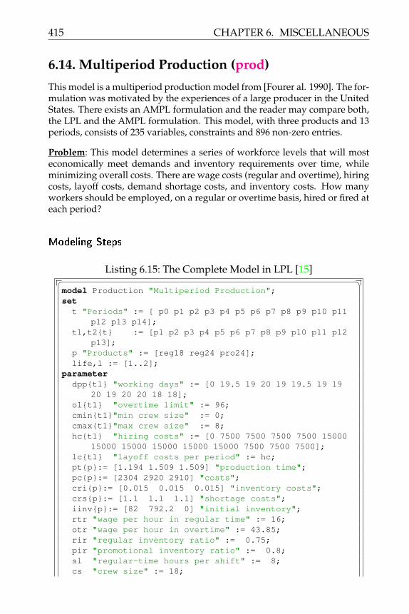
415 CHAPTER 6. MISCELLANEOUS

6.14. Multiperiod Production (prod)This model is a multiperiod production model from [Fourer al. 1990]. The for-mulation was motivated by the experiences of a large producer in the UnitedStates. There exists an AMPL formulation and the reader may compare both,the LPL and the AMPL formulation. This model, with three products and 13periods, consists of 235 variables, constraints and 896 non-zero entries.

Problem: This model determines a series of workforce levels that will mosteconomically meet demands and inventory requirements over time, whileminimizing overall costs. There are wage costs (regular and overtime), hiringcosts, layoff costs, demand shortage costs, and inventory costs. How manyworkers should be employed, on a regular or overtime basis, hired or fired ateach period?

Modeling Steps

Listing 6.15: The Complete Model in LPL [15]� �model Production "Multiperiod Production";set

t "Periods" := [ p0 p1 p2 p3 p4 p5 p6 p7 p8 p9 p10 p11p12 p13 p14];

t1,t2{t} := [p1 p2 p3 p4 p5 p6 p7 p8 p9 p10 p11 p12p13];

p "Products" := [reg18 reg24 pro24];life,l := [1..2];

parameterdpp{t1} "working days" := [0 19.5 19 20 19 19.5 19 19

20 19 20 20 18 18];ol{t1} "overtime limit" := 96;cmin{t1}"min crew size" := 0;cmax{t1}"max crew size" := 8;hc{t1} "hiring costs" := [0 7500 7500 7500 7500 15000

15000 15000 15000 15000 15000 7500 7500 7500];lc{t1} "layoff costs per period" := hc;pt{p}:= [1.194 1.509 1.509] "production time";pc{p}:= [2304 2920 2910] "costs";cri{p}:= [0.015 0.015 0.015] "inventory costs";crs{p}:= [1.1 1.1 1.1] "shortage costs";iinv{p}:= [82 792.2 0] "initial inventory";rtr "wage per hour in regular time" := 16;otr "wage per hour in overtime" := 43.85;rir "regular inventory ratio" := 0.75;pir "promotional inventory ratio" := 0.8;sl "regular-time hours per shift" := 8;cs "crew size" := 18;

CHAPTER 6. MISCELLANEOUS 416

iw "initial workforce" := 8;dem{t,p} "demand" := /

: reg18 reg24 pro24 :p1 63.8 1212 .p2 76 306.2 .p3 88.4 319 .p4 913.8 208.4 .p5 115 298 .p6 133.8 328.2 .p7 79.6 959.6 .p8 111 257.6 .p9 121.6 335.6 .p10 470 118 1102p11 78.4 284.8 .p12 99.4 970 .p13 140.4 343.8 .p14 63.8 1212 . /;

pro{t,p} "promoted products in a period (=1)" :=/ p1 reg24 1p4 reg18 1p7 reg24 1p10 reg18 1p10 pro24 1p13 reg24 1p14 reg24 1 /;

iil{t1,p}:=Max(iinv - sum{t2|t2<=t1} dem[t2,p],0) "initial inventory left";

minv{t in t1,p} := dem[t+1,p]*if(pro[t+1,p],pir,rir) "minimum inventory";

variableCrews{t|t<#t} "Average number of crews employed";Hire{t1} "Crews hired from previous to current

period";Layoff{t1} "Crews laid off from previous to current

period";Rprd{t1,p} "Regular production";Oprd{t1,p} "Overtime production";Inv{t1,p,life|life<t1} "Inventory";Shortage{t1,p} "Accumulated unsatisfied demand";

constraintrlim{t1}: sum{p} pt*Rprd <= sl*dpp[t1]*Crews[t1] "

Regular time limits";olim{t1}: sum{p} pt*Oprd <= ol[t1] "Overtime limits";empl0: Crews['p0'] = iw "initial crew level";empl{t1}: Crews[t1] = Crews[t1-1] + Hire[t1] - Layoff[

t1] "Crew levels";Bounds{t1}: cmin[t1] <= Crews[t1] <= cmax[t1] "Crew

limits";dreq{t1,p}: Rprd + Oprd + Shortage[t1,p] - Shortage[t1

-1,p]

417 CHAPTER 6. MISCELLANEOUS

+ sum{l} ( Inv[t1-1,p,l] - Inv[t1,p,l] ) = dem[t1,p]-Max(iil[t1,p],0)

"Demand requirement";ireq{t1,p}: sum{life} Inv + iil >= minv "Inventory

requirements";ilim1{t1,p}: Inv[t1,p,1] <= Rprd + Oprd "New-

inventory limits";alim{t1,p,l | t1>1 and l>1}: Inv <= Inv[t1-1,p,l-1] "

Inventory limits";minimize cost: sum{t1} (rtr*sl*dpp[t1]*cs*Crews[t1] + hc[

t1]*Hire[t1]+ lc[t1]*Layoff[t1]) + sum{t1,p} (otr*cs*pt*Oprd +

crs*pc*Shortage)+ sum{t1,p,life} cri*pc*Inv

"Regular wages+hired and layoff costs+overtimewages+shortage and inventory costs";

Write{t1}('\nperiod Crews Hire Layoff\n %5s%3d %3d %4d\n', t1,Crews[t1],Hire[

t1],Layoff[t1]);Writep(cost,Rprd,Oprd,Shortage,Inv);end� �

Model from: FOURER R. and GAY D.M. and KERNIGHAN B.W., [1990], AModeling Languagef for Mathematical Programming, in: Management Sci-ence, Vol. 36, p. 519ff.

CHAPTER 6. MISCELLANEOUS 418

6.15. Production and Planning (prodplan)

Problem: A small proction problem: ...

Modeling Steps

Listing 6.16: The Complete Model in LPL [15]� �model PRODPLAN "Production and Planning";set

product,p := [1..5];month ,m := [Jan,Feb,Mar,Apr,May,Jun];machine,r := [Grind,Vdrill,Hdrill,Boring,Planing];

parameterprice {p} := [ 10.00 6.00 8.00 4.00 11.00 ];time {r,p} := [

50 70 0 0 3010 20 0 30 020 0 80 0 05 3 0 7 100 0 1 0 5];

MaxSales {m,p} := [500 1000 300 300 800600 500 200 100 400300 600 200 200 500200 300 400 500 200400 100 500 100 1000500 500 100 300 1100];

DaysPerMonth := 6*4;HoursPerDay := 2*8;HoursPerMonth := HoursPerDay * DaysPerMonth ;MachineHours {m,r} := [ 3, 2, 3, 3, 3,

4, 2, 1, 3, 3,4, 2, 3, 2, 3,4, 1, 3, 3, 3,3, 1, 3, 3, 3,4, 2, 2, 3, 2 ];

InventoryCost := 0.50;variable

Sale {p,m};Produ {p,m};Invt {p,m};

constraintCapacity{m,r}: sum{p} time/100*Produ <= HoursPerMonth*

MachineHours;Balance{p,m}: Invt = Invt[p,m-1] + Produ - Sale;Bound {p,m} : Sale <= MaxSales;

419 CHAPTER 6. MISCELLANEOUS

InvtCapacity {p,m} : if(m='Jun' , Invt=50 , Invt<=100);maximize Contribution: sum{p,m} (price*Sale-InventoryCost

*Invt);Writep(Contribution,Sale,Produ,Invt);end� �

CHAPTER 6. MISCELLANEOUS 420

6.16. Production and Shipment Planning (prodship)

Problem: There are a number of plants, each manufacturing several prod-ucts. The products are shipped to various warehouses from where they aredistributed to demand-centers or customers. Each demand-center is suppliedfrom only one warehouse. The question is how much, and at which plants, toproduce a given commodity in order to meet the demand requirements at thedemand-centers while minimizing production and transportation costs. Fig-ure 6.4 gives a overview of the overall product flow, (The model was designedby: [16]).

Figure 6.4: Product Flow Description

Modeling Steps

1. ...

Listing 6.17: The Complete Model in LPL [15]� �

421 CHAPTER 6. MISCELLANEOUS

model ProdShip "Production and Shipment Planning";setplants,f "A set of plants (factories)";products,p "A set of products";warehouses,w "A set of warehouses";centers,c "A set of demand-centers";

parameterCAPACITY{f,p} "The quantity that can maximally be

produced";PCOST {f,p} "The production cost";SCOST{f,w} "The shipping cost (plant to warehouse)";TCOST{w,c} "The transshipping cost (warehouse to

centers)";DEMAND{c,p} "Demands at the centers";

variablePRODUCE{f,p|PCOST} [0..CAPACITY] "The quantity to

produce (cannot exceed the capacity)";SHIP{f,w,p|PCOST and SCOST} "The quantity to be

shipped";binary ASSIGN{w,c|TCOST} "=1, if the center is

assigned to the warehouse, otherwise 0";constraintPRODROW{f,p|PCOST} :sum{w} SHIP - PRODUCE = 0"All produced quantities must be shipped to the

warehouses";SHIPROW{f,w,p|SCOST}: sum{c} DEMAND*ASSIGN - sum{f}

SHIP = 0"The demands must be satisfied (nothing must be

stored)";CENTROW{c}: sum{w} ASSIGN = 1

"A center can be supplied from only one warehouse";minimize COST: sum{f,p} PCOST*PRODUCE + sum{f,w,p}

SCOST*SHIP+ sum{w,c} TCOST*(sum{p} DEMAND)*ASSIGN

"The overall cost, i.e. production, shipping andtransshipping cost";

----- data setsmodel data1;/* data1: OPT=3290215.695, Var:720, Const:601,Ints

:169,NonZeroes:12751, Density:2.9467% */

f := [1..5];p := [1..11];w := [1..10];c := [1..20];CAPACITY{f,p} := if(Rnd(0,1)<0.95 , Rnd(500,2200));PCOST{f,p} := if(CAPACITY , Rnd(200,300));SCOST{f,w} := if(Rnd(0,1)<0.95 , Rnd(1,20));TCOST{w,c} := if(Rnd(0,1)<0.90 , Rnd(15,70));DEMAND{c,p} := Rnd(20,100);

CHAPTER 6. MISCELLANEOUS 422

endmodel data2;/* data2: OPT= , Var:1613, Const:1521, Ints:181,

NonZeroes: 44071, density: 1.7963% */f := [1..13];p := [1..11];w := [1..10];c := [1..20];CAPACITY{f,p} := if(Rnd(0,1)<0.95 , Rnd(500,2200));PCOST{f,p} := if(CAPACITY , Rnd(200,300));SCOST{f,w} := if(Rnd(0,1)<0.95 , Rnd(1,20));TCOST{w,c} := if(Rnd(0,1)<0.90 , Rnd(15,70));DEMAND{c,p} := Rnd(20,100);/* different parametersCAPACITY{f,p} := if(Rnd(0,1)<0.95 , Rnd(500,2200));PCOST{f,p} := if(CAPACITY , Rnd(200,300));SCOST{f,w} := if(Rnd(0,1)<0.65 , Rnd(1,20));TCOST{w,c} := if(Rnd(0,1)<0.75 , Rnd(15,70));DEMAND{c,p} := Rnd(20,100); */

endmodel data3;f := [1..13];p := [1..20];w := [1..10];c := [1..20];CAPACITY{f,p} := if(Rnd(0,1)<0.95 , Rnd(500,2200));PCOST{f,p} := if(CAPACITY , Rnd(200,300));SCOST{f,w} := if(Rnd(0,1)<0.95 , Rnd(1,20));TCOST{w,c} := if(Rnd(0,1)<0.90 , Rnd(15,70));DEMAND{c,p} := Rnd(20,100);

endmodel data4;f := [ topeka ny ];p := [ chips nachos ];w := [ topeka ny ];c := [ east south west ];CAPACITY{f,p} := /

topeka chips 200topeka nachos 800ny chips 600/;

PCOST{f,p}:=/topeka chips 230topeka nachos 280ny chips 255 /;

SCOST{f,w} := /topeka topeka 1topeka ny 45ny ny 2ny topeka 45 /;

TCOST{w,c} := /

423 CHAPTER 6. MISCELLANEOUS

topeka east 60topeka south 30topeka west 40ny east 10ny south 30ny west 80 /;

DEMAND{c,p} := /east chips 200east nachos 50south chips 250south nachos 80west chips 150west nachos 300 /;

endmodel data;f := [1..10];p := [1..7];w := [1..20];c := [1..20];CAPACITY{f,p} := if(Rnd(0,1)<0.85 , Rnd(200,800));PCOST{f,p} := if(CAPACITY , Rnd(200,300));SCOST{f,w} := if(Rnd(0,1)<0.65 , Rnd(1,20));TCOST{w,c} := if(Rnd(0,1)<0.75 , Rnd(15,70));DEMAND{c,p} := Rnd(50,250);

endmodel output;Write('Total costs are: %15.2f\n', COST);Write('Assignment:\n warehouse assigned centers\

n\-------------------------------------\n');

Write{w}(' %6s %5s\n', w, {c|ASSIGN}c);Writep(PRODUCE,SHIP,ASSIGN);

endend� �

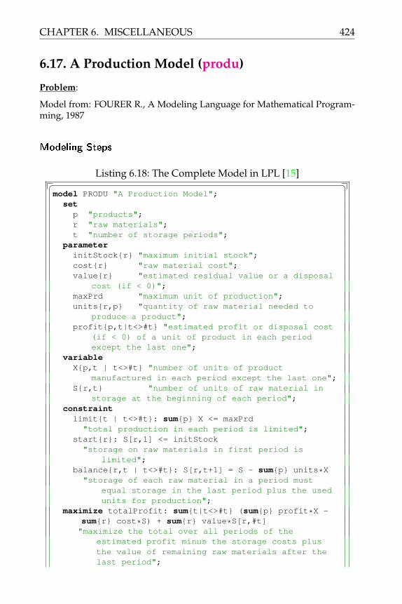
CHAPTER 6. MISCELLANEOUS 424

6.17. A Production Model (produ)

Problem:

Model from: FOURER R., A Modeling Language for Mathematical Program-ming, 1987

Modeling Steps

Listing 6.18: The Complete Model in LPL [15]� �model PRODU "A Production Model";

setp "products";r "raw materials";t "number of storage periods";

parameterinitStock{r} "maximum initial stock";cost{r} "raw material cost";value{r} "estimated residual value or a disposal

cost (if < 0)";maxPrd "maximum unit of production";units{r,p} "quantity of raw material needed to

produce a product";profit{p,t|t<>#t} "estimated profit or disposal cost

(if < 0) of a unit of product in each periodexcept the last one";

variableX{p,t | t<>#t} "number of units of product

manufactured in each period except the last one";S{r,t} "number of units of raw material in

storage at the beginning of each period";constraintlimit{t | t<>#t}: sum{p} X <= maxPrd

"total production in each period is limited";start{r}: S[r,1] <= initStock

"storage on raw materials in first period islimited";

balance{r,t | t<>#t}: S[r,t+1] = S - sum{p} units*X"storage of each raw material in a period must

equal storage in the last period plus the usedunits for production";

maximize totalProfit: sum{t|t<>#t} (sum{p} profit*X -sum{r} cost*S) + sum{r} value*S[r,#t]"maximize the total over all periods of the

estimated profit minus the storage costs plusthe value of remaining raw materials after thelast period";

425 CHAPTER 6. MISCELLANEOUS

Writep(totalProfit,X,S);model data "an model instance";t := [1..5];p := [nuts bolts washers];r := [nickel iron];initStock{r}:=[7.32 35.8];value{r}:=[-0.01 0.025];cost{r}:=[0.025 0.03];maxPrd := 123.7;profit{p,t} :=[1.73 1.8 1.6 2.2 .

1.82 1.9 1.7 2.5 .1.05 1.1 0.95 1.33 .];

units{r,p} := [0.21 0.17 0.080.79 0.83 0.92];

endend� �

CHAPTER 6. MISCELLANEOUS 426

6.18. Multiperodic Production Planning (product)

Problem: A company manufactures k ∈ K products (say three: P1, P2, P3)and has at its disposal h ∈ H machines (say three: M1, M2, M3) to producethem. It can undertake normal and overtime production and needs to planfor two time periods (say winter and summer). The products can be storedbetween periods, but the capacity is limited for each product. Any productleft over after the last period has very little resale value. Machine capacities,production time of a unit on a machine, selling prices, demand for each prod-uct are given. How should the company produce each product in order tofulfil all constraints? (This problem is from: [10]).

Modeling Steps

There are different ways of attacking the problem. One way is to begin withthe data.

1. Resale value r and storage cost s: they depend on the product types,hence we have rk and sk for each product type k.

2. Storage capacity u: supposing that each product type has its limits, thenwe have uk for each product type k.

3. Demand d and selling price: Suppose we have a different demand andprice for each product type k in each time period i (summer and win-ter), then this gives two tables di,k and pi,k.

4. The different machines h have different availability time a in the vari-ous production modes j (normal and overtime) and in the different timeperiods i. Hence the data are given in a three-dimensional table ai,j,h.

5. Each unit of product k manufatured at each machine h in each period iand under the different production modes j has different costs c. Thisis specified in a four-dimensional table ci,j,k,h.

6. Finally, each machine h needs a different time t to manufacture a unit ofa product k in each time period i under the different production modesj. Hence ti,j,k,h. (Of course, we might suppose that this time t does notdepend on production modes j neither on the time period i. In this casewe would have tk,h. The modeller has the liberty here to specify thedata, but it depends on the context. We choose a finer grid in the data.)

7. Now we might ask: what are the variables, the unknown quantities,to be calculated. Certainly we need to specify the quantity sold Z andstored Y of each product type k in each time period i. Hence we get Zi,k

and Yi,k.

427 CHAPTER 6. MISCELLANEOUS

8. Furthermore, we need the quatity produced X for each product k un-der the different modes j in each time period i manufactured by thedifferent machines h. Hence Xi,j,k,h.

9. We want to maximize profit, that is the value produced minus storagecosts minus the final resale value.

10. The value produced is (unit price minus unit cost) times quantity overall products in all periods, that is:

∑i,j,k,h(pi,k − ci,j,k,h) · Xi,j,k,h

11. The storage costs are: unit storage cost times storage quantity of allproducts in all period except the last. That is,

∑i,k|i<#i si,k · Yi,k.

12. The final resale value is∑

k(rk − p#i,k) · Y#i,k.

13. The constraints are as follows. The demand must be fulfilled: Zi,k ≥di,k. for each product type k in each time period i.

14. The storage in each period i and for each product is limited: Yi,k ≤ uk.

15. The machine availability is limited:∑

k ti,j,k,h · Xi,j,k,h ≤ ai,j,h. foreach machine h in each time period i and in each production mode j.

16. Finally, there is a balance of quantities for each product k in each timeperiod i: produced quantity plus stock at the beginning of the periodis equal to sold quantity plus stored quantity at the end of a period.Hence:

∑j,h Xi,j,k,h+Yi−1,k = Yi,k+Zi,k. The formulation is complete.

The pieces are put together and the complete model follows.

Listing 6.19: The Complete Model in LPL [15]� �model Production "Multiperodic Production Planning";

seti := [summer winter] "Time periods";j := [normal overtime] "Productionmodes";k := [p1 p2 p3] "Product types";h := [m1 m2 m3] "Machines";

parametert{i,j,k,h} "Machine hours used to produce a unit"

:= [4 7 3 5 6 . 6 6 .3 6 2 4 5 . 5 5 .5 8 4 6 7 . 7 7 .4 7 3 5 6 . 5 6 .];

c{i,j,k,h} "The production cost":= [2 4 1 3 3 . 4 2 .

3 5 2 4 4 . 5 3 .3 5 2 4 4 . 5 3 .4 6 3 5 5 . 6 4 .];

a{i,j,h} "Machine availability":= [100 100 40 80 90 30

110 110 50 90 100 40];

CHAPTER 6. MISCELLANEOUS 428

p{i,k} "Selling price" := [10 10 9 11 11 10];d{i,k} "Demand" := [25 30 30 30 25 25];s{k} "Storage cost" := [ 1 1 1 ];u{k} "Storage capacity" := [20 20 . ];r{k} "Final resale value" := [ 2 2 1 ];

variableX{i,j,h,k|t} "Quantity of product to be produced";Y{i,k} "Quantity of product to be stored at end of i"

;Z{i,k} "Quantity of product k sold";

constraintMACHINES{i,j,h}: sum{k} t*X <= a

"Machine capacity in hours";STOCK{k,i}: sum{j,h} X + Y[i-1,k] = Y + Z

"Product balances between periods";DEMAND{i,k}: Z >= d

"Demands to be satisfied";BOUND{i,k|i<#i}: Y <= u

"Upper bound on storage";maximize Profit: sum{i,j,k,h}(p-c)*X - sum{k,i|i<#i}s*Y

+ sum{k}(-r+p[#i,k])*Y[#i,k]"Revenue minus production costs minus storage costs";

parameter Sx{i,k}:=sum{j,h}X;Writep(Sx,Y,Z);

end� �Further Comments: This formulation is a mathematical system of 27 equa-tions and inequations and 40 variables with a maximizing function. We callthis a linear program (LP). It can be solved efficiently with the well-knownsimplex method. The method finds the best values for the unknowns X, Y,and Z.

Solution: The solution is written as tables of sum{j,h} X, Y, and Z. The threeresulting tables are as follows:

Sx{i,k}p1 p2 p3

summer 45.00 32.17 30.00winter 51.79 22.83 25.00

Y{i,k}p1 p2

summer 20.00 2.17winter 41.79

Z{i,k}p1 p2 p3

429 CHAPTER 6. MISCELLANEOUS

summer 25.00 30.00 30.00winter 30.00 25.00 25.00

The result says that 45 and 51.79 units are produced of product p1 in twoperiods where 20 are stored after the first period and 41.79 after the secondperiod. 25 units are sold in the first period and 30 in the second. Hence 41.79are left to be sold at a discount price at the end. Only 2.16 units are stored ofthe product p2 after the first period and nothing after the second period, andnothing is stored of product p3.

Question (Answer see ??)

1. Run the model. What is the profit?

2. What happens if the storage has unlimited capacity?

Answer (Question see 6.8)

1. Click on the link at the beginning of the model specification. Then sendthe model to the Internet solver. It returns 1842.7714.

2. Remove the storage bounding constraint BOUND and solve again. Thereis almost no change in the result.

CHAPTER 6. MISCELLANEOUS 430

6.19. Multiperiod Production Scheduling (schedule)

Problem: Solve the following production planning problem by specifyinghow many units of product should be manufactured each period in orderto minimize the sum of inventory holding c and production costs. .. There are20 units of product in inventory at the start of period 1. Smythe W.R.,Johnson

ReferencesL.A..,1966,p.202

Listing 6.20: The Complete Model in LPL [15]� �model SCHEDULE "Multiperiod Production Scheduling";set

t := [1..5]; -- periodsc := [ regular,forallTime,inventory ];

parameterrc{t} := [120 100 90 140 90]; -- Regular Time

Capacity, Unitsov{t} := [ 30 40 20 40 60]; -- Overtime

Capacity, Unitspr{t} := [110 160 100 100 150]; -- Production

Requirements, Unitsco{c,t} :=

[12 12 16 10 11 -- Regular Time Cost perUnit

15 16 18 14 14 -- Overtime Cost per Unit1 1 1 1 1]; -- Inventory costs from

period i to i+1variable

PRODUCT{c,t};constraint

init: PRODUCT['inventory',1] = 20 "initial inventory";prodcapa{t}: PRODUCT['regular',t] <= rc "production

capacity";capa{t}: PRODUCT['forallTime',t] <= ov "foralltime

capacity";const{t}: sum{c} PRODUCT - PRODUCT['inventory',t+1] =

pr;minimize costs: sum{c,t} co * PRODUCT;Writep(costs,PRODUCT,co);end� �

431 CHAPTER 6. MISCELLANEOUS

6.20. A Round Trip Problem (vacation)

Problem: Visit all towns at least once at minimal costs

Listing 6.21: The Complete Model in LPL [15]� �model VACATION "A Round Trip Problem";set

i,j:=[GraniteCity StGeorges Cutler Chester Denver];parameter

Miles{i,j} "distances between towns in miles" :=[ . 1600 90 85 1000

1620 . 2000 2300 80095 2005 . 35 1300

100 2400 40 . 18001500 825 1250 2000 . ];

UnitCost "costs per unit/mile" := 1;integer variable VISITS{i,j | i<>j};constraint

V{j} "Visit each location at least once" : sum{i}VISITS[i,j] >= 1;

L{i} "Leave all location at most once" : sum{j}VISITS[i,j] <= 1;

T{i,j | j>i} "Insure a unique cycle tour" : VISITS[i,j]+ VISITS[j,i] <= 1;

minimize cost: sum{i,j} Miles[i,j]*UnitCost*VISITS[i,j];Writep(VISITS,cost);end� �

CHAPTER 6. MISCELLANEOUS 432

6.21. Multi-period Blending Problem (xpress)

Problem: The following is a multi-period blending model. Production of ametal smelter is to be planned over each of the 30 weeks. Unit productioncosts increase with production rate. The smelted metal must satisfy certainquality requirements and metal produced in one week may be stored for salein subsequent weeks. Objective: find the cheapest blend of ores to smelt andplan production to trade off production and storage cost.

Modeling Steps

Listing 6.22: The Complete Model in LPL [15]� �model xpress "Multi-period Blending Problem";

seti,nweeks := [1..30];nores := [1.. 5];nlin := [1..10];nqual := [1..10];

variablemetal{nweeks};diff{nweeks};ore{nores,nweeks};lin{nlin,nweeks};stock{nweeks};

parameter -- choose random datademand{nweeks} := Rnd(1,10);Myield{nores} := Rnd(2,2000);qual{nqual,nores} := Rnd(1000,3000);lowerq{nqual} := Rnd(20,30);upperq{nqual} := Rnd(1000,5000);orecst{nores} := Rnd(1,90);orebnd{nores} := Rnd(1000,2000);

prdlvl{nlin} := [0,10,20,30,40,50, 70,100,200, 300];prdcst{nlin} := [0, 5,15,30,50,80,160,295,795,1345];D{nweeks} := / 1 1 /;maxstock := 1000;maxdiff := 300;curstock := 10;curmetal := 100;

constraintyield{nweeks}: sum{nores} Myield*ore - metal = 0;lqual{nqual,nweeks}: sum{nores} (qual-lowerq)*ore >=

0;uqual{nqual,nweeks}: sum{nores} (qual-upperq)*ore <=

0;produ{nweeks}: sum{nlin} prdlvl*lin - metal = 0;

433 CHAPTER 6. MISCELLANEOUS

convex{nweeks}: sum{nlin} lin = 1;smooth{nweeks }:

metal - sum{i} metal[i-1] + diff = D*curmetal;malbal{nweeks}:

-stock + metal + sum{i} stock[i-1]>= demand - D*curstock;

StockBound{nweeks}: stock <= maxstock;DiffBounds{nweeks}: max(0,-maxdiff) <= diff <=

maxdiff;OreBound{nores,nweeks}: ore <= orebnd;

minimize TotalCost: sum{nweeks,nores} orecst/1000*ore+ sum{nweeks,nlin} prdcst/1000*lin;

Writep(TotalCost,metal,diff,stock,ore,lin);end� �

Further Comments: The XPRESS-LP formulation: (copied from: "XPRESS-LP,a prospectus of Dash Associates").

. Multiperiod production/inventory furnace blending problem

.constraint smelter . gives the model a name.LET nweeks = 30 . number of periodsLET nores = 5 . number of ores can buyLET nqual = 10 . number of ore qualitiesLET nlin = 10 . number of linearisation points.VARIABLES . define decision variablesmetal(nweeks) . final metal productiondiff(nweeks) . change in prod level one week to nextore(nores,nweeks) . raw ores to buylin(nlin,nweeks) . production linearisation variablesstock(nweeks) . stocks of smelted metal.TABLES . define main data tablesdemand(nweeks) . weekly demandqual(nqual,nores) . ore qualities (first is metal yield)lowerq(nqual) . lower limits on metal qualitiesupperq(nqual) . upper limits on metal qualitiesorecst(nores) . ore costprdlvl(nlin) . metal production levelprdcst(nlin) . production cost at prdlvlorebnd(nores) . upper bounds on ore purchasesmaxstock . maximum metal stock levelD(nweeks) . switch array.

CHAPTER 6. MISCELLANEOUS 434

DISKDATA . input data to major tablesdemand(1) = xpress.demqual(1,1) = xpress.qullowerq(1) = xpress.lquupperq(1) = xpress.uquorecst(1) = xpress.ocsorebnd(1) = xpress.orbDATA . data assigned explicitlyprdlvl(1) = 0,10,20,30,40,50, 70,100,200, 300prdcst(1) = 0, 5,15,30,50,80,160,295,795,1345D(1) = 1 . switch - all other D(t) are zeromaxstock = 100 . maximum stock levelmaxdiff = 30 . maximum change in production levelcurstock = 10 . current stock levelcurmetal = 100 . current metal production level.CONSTRAINTS . total cost and problem constraints.. total cost (to be minimized).totalcst: sum(t=1:nweeks,j=1:nores) &

(orecst(j)/1000*ore(j,t) &+ sum(t=1:nweeks,i=1:nlin) (prdcst(i)/1000*lin(i,t) $

.

. metal yield

.yield(t=1:nweeks): sum(j=1:nores) qual(1,j)*ore(j,t) &

- metal(t) = 0.. lower quality limits (where applicable).qual(k=2:nqual,t=1:nweeks | lowerq(k).ne.0): &

sum(j=1:nores) (qual(k,j)-lowerq(k))*ore(j,t) > 0. upper quality limits (where applicable).uqual(k=2:nqual,t=1:nweeks) | upperq(k).ne.0): &

sum(j=1:nores) (qual(k,j)-upperq(k))*ore(j,t) < 0.. production level (so can have piecewise linear cost).prod(t=1:nweeks): sum(i=1:nlin) prdlvl(i)*lin(i,t) &

- metal(t) = 0.convex(t=1:nweeks): sum(i=1:nlin) lin(i,t) = 1.

435 CHAPTER 6. MISCELLANEOUS

. production smoothing

.smooth(t=1:nweeks): &

metal(t) - sum(|t.ne.1) metal(t-1) + diff(t) &= D(t)*curmetal

.

. material balance and satisfy demand

.matbal(t=1:nweeks): &

-stock(t) + metal(t) + sum(|t.ne.1) stock(t-1) &> demand(t) - D(t)*curstock

.BOUNDS . simple bounds.stock(t=1:nweeks) < maxstock . stock leveldiff(t=1:nweeks) < maxdiff . decrease in productiondiff(t=1:nweeks) > -maxdiff . increase in productionore(j=1:nores,t=1:nweeks) < ore purchases.GENERATE . generate the matrix. end of XPRESS-LP formulation

Model from: DASH ASS. (XPRESS-LP is a trademark of DASH ASSOCIATES,Northants, UK).

BIBLIOGRAPHY

[1] R. Borndoerfer, M. Groetschel, and A. Loebel. Alcuin’s TransportationProblem and Integer Programming. Konrad Zuse Zentrum for Informa-tionstechnik, Berlin, 1995.

[2] R. Bosch. Mind Sharpener. OPTIMA MPS Newsletter, January 2000.

[3] J. Bracken and G.P. McCormick. Selected Applications of Nonlinear Pro-gramming. John Wiley and Sons, New York, 1968.

[4] A. Brooke, D. Kendrick, and A. Meeraus. GAMS: A User’s Guide. TheScientific Press, Redwood City, California, 1988.

[5] L. Cesari. Optimization – Theory and Applications. Springer Verlag, 1983.

[6] Pulleyblank W.R. Schrijver A. Cook W.J., Cunningham W.H. Combinato-rial Optimization. John Wiley and Sons, Inc., 1998.

[7] H. Dahl, A. Meeraus, and S.A. Zenios. Some Financial OptimizationModels: Risk Management. in: Zenios, S.A., ed, Financial Optimization.Cambridge University Press, New York, 1993.

[8] G.B. Dantzig. Linear Programming and Extensions. Princeton UniversityPress, Princeton, New Jersey, 1963.

[9] E.D. Dolan and J.J. More. Benchmarking Optimization Software withCOPS., Tech. Report. Mathematics and Computer Science Division„2000.

[10] E.F.D. Ellison and G. Mitra. UIMP: User Interface for Mathematical Pro-gramming. ACM Transaction on Mathematical Software, 8:3:229–255, 1982.

[11] R. Fourer, D.M. Gay, and B.W. Kernighan. AMPL: A Modelling Language

437

Bibliography 438

for Mathematical Programming. Duxbury Press/Brooks/Cole Publ. Co.,second edition, 2003.

[12] Hillier F.S. and Liebermann G.J. Introduction to Operations Research.McGraw-Hill, 6rd ed., 1999.

[13] Ch. Guéret, Ch. Prins, and M. Sevaux. Programmation linéaire, 65 prob-lèmes d’optimisation modélisés et résolus avec Visual Xpress. Eyrolles, 2000.

[14] H-O. Günther and H. Tempelmeier. Produktion und Logistik. Springer,Berlin, 2002.

[15] T. Hürlimann. Reference Manual for the LPL Modelling Language, mostrecent version. lpl.virtual-optima.com/lpl/doc/manual.pdf.

[16] E.L. Johnson. Modeling and Strong Linear Programs for Mixed Integer Pro-gramming, pages 1–43. NATO ASI Series F, Vol. 51, Springer, 1989.

[17] D. Kendrick. Caution and Probing in a Macroeconomic Model. Journalof Economic Dynamics and Control 4, 2, 1982.

[18] Murty K.G. Operations Research: Deterministic Optimization Models. Pren-tice Hall, 1994.

[19] G.P. Kutcher, A. Meeraus, and G.T. O’Mara. Agriculture Sector and Pol-icy Models. The World Bank, 1988.

[20] G.P. Kutcher and P.L. Scandizzo. The Agricultural Economy of North-east Brazil. The Johns Hopkins University Press, Baltimore and London,1981.

[21] Seiford L.M. and Thall R.M. Recent developments in DEA: the mathe-matical programming approach to frontier analysis. Journal of Economet-rics, Vol 46, p. 7–38, 1990.

[22] G. Polya. How To Solve It. Penguin Books 1990, London, 1957.

[23] Shapiro RD. Optimization models for planning and allocation. John WileySons, 1984.

[24] Ahuja R.K., Magnanti T.L., and Orlin J.B. Network Flows, Theory, Algo-rithms, and Applications. Prentice Hall, 1993.

[25] R.E. Rosenthal. Tutorial of GAMS in: GAMS: A User’s Guide. The ScientificPress, Redwood City, California, 1988.

[26] Heipcke S. Applications of optimization with Xpress. dash optimization,2000,www.maths.ed.ac.uk/hall/Xpress/FICO_Docs/Xpress-booka4.pdfA translation of [13].

439 Bibliography

[27] Wiens T.B. The Economics of High-yield Agriculture, in: China: Triple-Cropping at the Baimano Peoples’ Commune. The World Bank, Wash-ington DC, 1985.

[28] H.P. Williams. Model Building in Mathematical Programming. John Wiley,Third Edition Revisted, 1993.

[29] H.P. Williams. Model Building in Mathematical Programming. John Wiley,Fifth Edition, 2013.

[30] W.L. Winston. Introduction to mathematical programming, applications andalgorithms. Duxbury Press, second edition, 1995.