August, 1978 FTReport No. Env. E. 59-78-2

Mathematical Modelof the Fluidized BedBiofilm Reactor

Leo T. MulcahyEnrique J. La Motta

Division of Water Pollution ControlMassachusetts Water Resources CommissionContract Number MDWPC 76-1011)

ENVIRONMENTAL ENGINEERING PROGRAM

DEPARTMENT OF CIVIL ENGINEERING

UNIVERSITY OF MASSACHUSETTS

AMHERST, MASSACHUSETTS 01003.

MATHEMATICAL MODEL

OF THE

FLUIDIZED BED BIOFILM REACTOR

By

Leo T. MulcahyResearch Assistant

Enrique J. La MottaAssistant Professor of Civil Engineering

Division of Water Pollution ControlMassachusetts Water Resources Commission

Contract Number MDWPC 76-10(1)

Environmental Engineering ProgramDepartment of Civil Engineering

University of MassachusettsAmherst, Massachusetts 01003

August, 1978

ieo

ii

ACKNOWLEDGEMENTS

This report is a reproduction of Dr. Leo T. Mulcahy's PhD

dissertation, which was directed by Dr. Enrique J. La Motta,

Chairman of the Dissertation Committee. The other members of this

committee were Dr. E. E. Lindsey (Chemical Engineering and Civil

Engineering Departments) and Dr. R. L. Laurence (Chemical Engineering

Department).

This research was performed in part with support from the

Department of Civil Engineering, which awarded teaching assistantships

and associateships to L. T. Mulcahy, and in part with support from

the Massachusetts Division of Water Pollution Control, Research and

Demonstration Project No. 76-10(1).

ENGINEERING RELEVANCE

Although the fluidized bed biofilm reactor (FBBR) has been

extensively used in fermentation engineering for several years, its

application to wastewater treatment is recent, and it is still in the

experimental stage. The potential offered by this novel technique is

great: Pollutant removal can be achieved with high efficiency using

hydraulic detention times which are a fraction of those commonly used

in conventional units. This is obviously reflected on significant

savings in initial plant costs, and on exceptional flexibility in

plant expansions.

A rational design of the FBBR requires a thorough understanding

of the phenomena taking place in the unit. Although there is

abundant literature describing the behavior of gas-solid fluidized

beds, liquid-solid systems have not been studied in such detail. Thus,

there is a paucity of information regarding process behavior and process

design equations.

Modeling the FBBR must include a mathematical description of the

physical behavior of the unit, a model of the heterogeneous kinetics

of the reaction, and a mathematical model linking both physical and

biochemical phenomena. The study described in this report is a

first attempt to tackle this complex problem. As such, it must include

simplifications, such as using uniform particle size and constant

pollutant loading, among others.

Once this first attempt is shown to successfully describe the

process, the simplifications mentioned above will have to be eliminated

IV

to obtain a more complex model, which will describe the performance

of full scale units. It is hoped that the simplified model presented

herein will provide a good basis for other researchers and engineers

to attempt the more complex model of the FBBR.

Enrique 0. La Motta, PhDAssistant Professor ofCivil Engineering

ABSTRACT

Mathematical Model of the Fluidized Bed Biofilm Reactor

(June 1978)

Leo Thomas Mulcahy, B.E., Manhattan College

M.S., Ph.D., University of Massachusetts, Amherst

Directed by: Dr. Enrique LaMotta

The fluidized bed biofilm reactor is a novel biological waste-

water treatment process. The use of small, fluidized particles in

the reactor affords growth support surface an order of magnitude

greater than conventional biofilms systems, while avoiding clogging

problems which would be encountered under fixed bed operation. This

allows retention of high biomass concentration within the reactor.

This high biomass concentration, in turn, translates to substrate

conversion efficiencies an order of magnitude greater than possible

in conventional biological reactors.

The primary objective of this research has been the development

of a mathematical model of the fluidized bed biofilm reactor. The

mathematical model has two major subdivisions. The first predicts

biomass holdup and biofilm thickness within the reactor using drag

vi

coefficient and bed expansion correlations developed as part of this

research. The second predicts mass transport-affected substrate con-

version by biofilm covering individual support particles. The intrin-

sic kinetic coefficients and effective diffusivity for nitrate limited

biofilm denitrification, used as input to this portion of the model,

were determined in an independent study using a rotating disk bio-

film reactor.

Biomass holdup, biofilm thickness, and nitrate profiles observed

in a laboratory fluidized bed biofilm reactor were compared with

simulated results obtained using the mathematical model. Good agree-

ment between observed and simulated results was obtained, with closest

agreement obtained for biofilm thicknesses under 300 microns.

It was found that the most significant parameter affecting sub-

strate conversion efficiency in a FBBR is biofilm thickness. It was

further determined that biofilm thickness, and thus FBBR performance,

can be regulated through specification of five design parameters:

1) Expanded bed height, HD;• b2) Reactor area perpendicular to flow, A;

3) Support media density, pm;

4) Support media diameter, d ;m5) Total volume of support media in the reactor, V .

vi i

The mathematical model developed as part of this research fur-

nishes a rational basis for selection of design parameters such that

FBBR performance is optimized.

A chapter on engineering applications of the mathematical model

has been included in the dissertation. This chapter provides back-

ground for the selection of an optimum biofilm thickness at which

to operate a fluidized bed biofilm reactor. Figures are presented

which allow graphical determination of FBBR design parameters such

that a desired operating biofilm thickness is obtained. These figures

are also used to assess the effect of changes in inflow rate on FBBR

bed expansion. This information provides a rational basis for the

determination of FBBR flow equalization requirements. In addition,

reactor freeboard requirements may be assessed, graphically, using

these figures.

vm

TABLE OF CONTENTS

Chapter Page

Title Page " i

Copyright ii

Approval iii

Dedication. . . . iv

Acknowledgement v

Abstract vi

Table of Contents ix

List of Tables xii

List of Figures xiii

Nomenclature xvii

I INTRODUCTION T

II RESEARCH OBJECTIVES 5

III FLUIDIZED BED BIOFILM REACTOR-BACKGROUND 6

3.1 Flow Models 18

3.2 Biomass Holdup - Fluidization 18

3.3 Substrate Conversion by Biological Films 49

3.3.1 External Mass Transfer 51

3.3.2 Internal Mass Transfer 58

3.3.3 Substrate Conversion Reaction 68

3.3.4 Biological Denitrification 73

IV FLUIDIZED BED BIOFILM REACTOR - MODEL DEVELOPMENT ... 78

4.1 An Overview of the Model 78

4.2 Fluidization - Bed Porosity and Biofilm Thickness. 86

ix

Table of Contents Continued...

Chapter Page

4.3 Substrate Conversion - Biofilm Effectiveness. . . 94

4.4 A Summary of the Model 101

V EXPERIMENTAL PROGRAM 105

5.1 Rotating Disk Reactor-Intrinsic Rate Constants andEffective Diffusivity 106

5.1.1 Materials and Methods 106

5.1.2. Theoretical Analysis 117

5.1.3 Results and Dissussion 123

5.2 Fluidized Bed Biofilm Reactor - Bed Expansion . . 133

5.2.1 Materials and Methods 133

5.2.2 Results and Discussion 143

5.3 Fluidized Bed Biofilm Reactor - Bioparticle Term-inal Velocity 148

5.3.1 Materials and Methods 148

5.3.2 Results and Discussion 150

5.4 Fluidized Bed Biofilm Reactor - Biomass Holdup andNitrate Profiles 152

5.4.1 Materials and Methods 152

5.4.2 Results and Discussion 154

VI ENGINEERING APPLICATIONS 159

VII SUMMARY, CONCLUSIONS AND RECOMMENDATIONS 184

Table of Contents Continued...

Chapter

Bibliography.

Appendix I

Appendix II

Appendix III

Appendix IV

Numerical Solution for Biofilm Effec-tiveness (Spherical Coordinates) . . .

Numerical Solution of the FBBR Flow Eq-uation

Numerical Solution for Biofilm Effective-ness (Rectangular Coordinates) . . . .

Experimental Data

Page

188

200

204

216

219

XI

LIST OF TABLES

Tables Page

3.1 Mathematical models and techniques used in attempts atthe theoretical calculation of drag forces in multipar-ticle systems 36

4.1 FBBR model input parameters and correlations 102

5.1 Literature zero order denitrification rate data 131

5.2 FBBR - Numerical values for input parameters 155

6.1 FBBR model computer output for Example 4 173

XII

LIST OF FIGURES

Figure Page

3.1 Reactor response to pulse inputs of a conservativematerial 20

3.2 Forces acting on a fluidized particle 29

3.3 Correlation of drag coefficient vs Reynolds number for asingle solid sphere 30

3.4 (Re/CQ)1/3 vs (Re CQ)

1/3 for a single solid sphere. . . 32

3.5 Drag coefficient as a function of Reynolds number andparticle sphericity 44

3.6 Hypothetical expansion curves based on apparent and ef-fective porosities 48

3.7 Sketch of a biofilvn showing external and internal sub-strate concentration gradients 52

3.8 Reaction rate versus substrate concentration for Mich-aetis-Menten kinetics .70

3.9 Reaction rate versus substrate concentration for discon-tinuous linear kinetics 71

3.10 Effect of pH on denitrification rate 76

xm

List of Figures Continued...

Figure Page

4.1 Differential element within a FBBR 79

4.2 .Flow chart of the bed fluidization algorithm 88

4.3 Schematic of a bioparticle 95

4.4 Block diagram of the FBBR model 104

5.1 Schematic of the laboratory rotating disk reactor . . 109

5.2 Photograph of the laboratory rotating disk reactor. . 110

5.3 Schematic of the rotating growth-support disk . . . . Ill

5.4 Differential biofilm element 119

5.5 The effect of disk rotational speed on external masstransfer limitations 125

5.6 Lineweaver-Burk plot of the RDR data 127

5.7 Lineweaver-Burk plot of the intrinsic RDR data. . . . 128

5.8 Schematic of the laboratory FBBR 134

5.9 Photograph of the laboratory FBBR 135

xiv

list of Figures Continued...

Figure Page

5.10 Schematic of the FBBR feed vessel - clarifier. ... 137

5.11 Typical FBBR bed expansion data 142

5.12 Expansion index versus Reynolds number; a log-logplot 144

5.13 Biofilm V.S. density versus biofilm thickness. ... 147

5.14 Log-log plot of drag coefficient vs Reynolds number. 151

5.15 Observed and predicted nitrate profiles for the lab-oratory FBBR 156

5.16 Observed and predicted nitrate profiles for the lab-oratory FBBR 157

5.17 Observed and predicted nitrate profiles for the lab-oratory FBBR 158

6.1 The effect of equilibrium biofilm thickness and super-ficial velocity on FBBR total volatile solids concen-tration 162

6.2 The effect of biofilm thickness on effective volatilesolids concentration 164

6.3 The effect of equilibrium biofilm thickness on FBBRtotal V.S. and effectiveness factor 166

xv

List of Figures Continued...

Figure Pa9e

6.4 The effect of bulk-liquid substrate concentrationon FBBR effective volatile solids concentration , . 167

6.5 The effect of biofilm thickness on nitrate conver-sion 170

6.6 The effect of biofilm thickness on FBBR bed expan-sion 172

6.7 Effect of support media density on effective volatilesolids concentration 179

6.8 Effect of support media diameter on effective vola-tile solids concentration 180

6.9 Effect of support media density on FBBR bed expan-sion 182

6.10 Effect of support media dtameter on FBBR bed expan-sion 183

Al- Comparisons of nitrate profiles, biomass holdups, andA10 biofilm thicknesses observed in the laboratory FBBR

and predicted by the FBBR model for each of the twentyexperimental runs 250

xvi

N O M E N C L A T U R E

A = reactor area perpendicular to flow

AT = disk biofilm total surface area

B = dimension!ess substrate concentration = S./S j

Bi = modified Biot number = kc<$/DSB

Bo = Bodenstein number = Dz/HnU

c = tracer concentration

c0 = tracer concentration at reactor inlet

C - biofilm dimensionless substrate concentration = S/S.

CD = drag coefficient

Ct = reactor exit concentration

Cy = solids volume fraction

d-i, dg = diameters defined in Eq. 3.41

da, db = diameters defined in Eq. 3.36

djp - support medium diameter

dD = bioparticle diameter

D = column diameter

DSB = diffusivity of species S through biofilm B

DSL ~ diffusivity of species S through liquid L

Dz = axial dispersion coefficient

Et = reactor exit age distribution

f(e) - correction factor =

FB = buoyancy force

xvi i

FD = drag force on a particle in a swarm

FDj = drag force on an isolated particle

Fo -' gravity force

g = gravity acceleration constant

g(e) = porosity correction factori 2Ga = Galileo number = dp* (ps - p|_) pL g /v

HB = expanded bed height

k - maximum substrate reaction rate

k_ = mass transfer coefficientO

A

k = zero order reaction rate

k1 = k/Ks

K = coefficient in Eq. 3.22

K-j, K2 = coefficients in Eq. 3.23•5

Kp - shape factor - Tr/6 (da/d^)

K$ = Michaelis-Menten constant

K1 = volume of solids plus immobilized fluid per unit solids

volume

L = reactor length

n = bed expansion index

na = apparent bed expansion index

n = effective bed expansion index

N = number of tanks-in-series

N = dispersive flux in the I direction

xvi ii

N1 = diffusional flux defined in Eq. 3.43

Pe = Peclet number = dpuR/Dsu

Pe* - axial Peclet number = dpU/Dz

Q = volumetric flowrate

r = Moparticle radial coordinate

Re - Reynolds number = dpUp|_/p

ReMp = minimum fluidization Re = dpU^pp./p

Ret - terminal Re = dpUtp|_/y

RT = intrinsic reaction rate per unit biofilm volume

R0 - = observed reaction rate per unit biofilm volume

RV = reaction rate per unit reactor volume

R = reaction rate defined in Eq. 3.55

S = substrate concentration

Sc - Schmidt number = y/D p.OL *-

Sh = Sherwood number = kCdp/Ds|_

St = Stanton number = kc e/U

S-j, $2 = surface areas defined in Eq. 3.41

S. = bulk-liquid substrate concentration

Sf = substrate feed concentration

Sp = projected particle area

S = substrate concentration at the liquid-biofilm interfaceO

t = time

T = temperature

xix

U = superficial liquid velocity = Q/A

U.j - velocity defined in Eq. 3.24

UR - relative particle-liquid velocity

Ut ~ particle terminal velocity

Vg = total biomass volume in FBBR

VM = total support media volume in FBBR

Vp = particle volume

Vs - total solids volume in FBBR

W = coefficient in Eq. 3.5

x = dimensionless bioparticle radial coordinate defined for

Eq. 4.34

X = volatile solids concentration in FBBR

XA = effective volatile solids concentration defined in Eq. 6.1

Xc - substrate conversion defined in Eq. 5.9

Y = dimensionless axial coordinate = Z/Hg

Z = axial coordinate

GREEK

Y - Ks/Sb

6 = biofilm thickness

e = FBBR bed porosity

ea = apparent bed porosity defined in Eq. 3.38

xx

E = effective bed porosity defined in Eq. 3.39

n = effectiveness factor

nj = intraphase effectiveness factor

n0 = overall effectiveness factor

M = liquid viscosity

y = apparent suspension viscosityc-

£ = V26

pg - biofilm volatile solids density

pgw = biofilm wet density

p, = liquid density

ps = particle density

02 = variance of residence time distribution

T - space time - reactor volume / Q

4T - Thiele-type modulus defined for Eq. 4.34

ij> = particle sphericity

0 = Ks'sblz=0

XXI

C H A P T E R I

INTRODUCTION

A surface in contact with a nutrient medium containing micro-

organisms, will eventually become biologically active. That is, the

surface will, in time, become covered with biofilm due to the adhesion

of micro-organisms from the bulk-fluid. This phenomenon forms the

cornerstone of the industrially important processes which utilize

biofilms. Examples include the trickling filter wastewater treatment

process, the "quick" vinegar process (in), animal tissue culture

(m), and bacterial leaching (136).

Growth support media within conventional biofilm reactors are

fixed in space either by gravity or by direct mechanical attachment

to the reactor shell.

In contrast, the reactor which is the topic of this study retains

growth support media in suspension by drag forces exerted by the up-

ward flow of the nutrient medium. Particles within such a reactor

are said to be fluidized, and the reactor will be refered to as a

fluidized bed biofilm reactor or FBBR. Particles within the FBBR are

no longer fixed in space but free to move under the influence of the

passing fluid.

The fluidized mode of operation allows use of small support

particles while avoiding clogging problems which would be encountered

under packed bed operation. The resultant available growth surface

1

within a FBBR is more than an order of magnitude greater than prac-

tical in a fixed bed reactor; this allows retention of high biomass

concentrations within the fluidized reactor. Jeris and Owens (62)

have reported volatile solids concentrations between 30,000 and

40,000 mg/1 for pilot-scale wastewater treatment studies using FBBR's

These high biomass concentrations translate to substrate conversion

efficiencies an order of magnitude greater than possible in conven-

tional biological reactors (63).

While the potential of fluidization technology to biological

process industries has been clearly demonstrated, application of this

technology to full scale use remains in the developmental stage.

Development of the fluidized bed biofilm reactor can be aided

by a mathematical model of the process, which incorporates signifi-

cant features of the system's behavior. This model should be .able to

assess the combined effects of biochemical rate processes and phys-

ical phenomena, such as diffusion, on the performance of the system.

The primary objective of this research is the developemnt of a

mathematical model of the fluidized bed biofilm reactor. The model,

which will be presented in later sections of this dissertation, has

two major subdivisions. The first, based on an analysis of FBBR!

fluidization mechanics, predicts biomass holdup (i.e. biomass con-

centration) within the reactor. Specifically, the model estimates

the equilibrium biofilm thickness and volumetric concentration of

biologically active particles which corresponds to a given set of

operating conditions. The second model subdivision calculates the

rate of substrate conversion by individual biologically active part-

icles within a FBBR. Limitations on reaction rate imposed by exter-

nal and internal (to the biofilm) transport phenomena are included

in this analysis.

In order to calculate the transport-affected rate of substrate

conversion by a biologically active particle, it is first necessary

that the effective diffusivity and the kinetic coefficients intrinsic

to the system be specified. As a paucity of such data exists in the

literature, it was necessary to determine these intrinsic parameters

experimentally. A rotating disk reactor (RDR) was used for this

purpose. This reactor configuration was selected because it offers

a uniformly accessible reaction surface which allows a clearer dif-

ferentiation of the major steps involved in substrate conversion by

biofilms.

Finally, the reaction used in this study of the fluidized bed

biofilm reactor was biological denitrification. This reaction was

chosen 'for several reasons. First, biological denitrification is

among the most efficient and economical methods for nitrate removal

from wastewaters. Second, there is substantial evidence in the lit-

erature that biofilm denitrification is a feasible process (45. 124,

110, 67> 13l)> and more specifically, that biological denitrification

in fluidized bed biofllm reactors is feasible (62, 63). And third,

the required apparatus is relatively simple when compared to that

needed for biochemical reactions such as carbonaceous oxidation or

nitrification, which require oxygenation.

C H A P T E R I I

RESEARCH OBJECTIVES

Based on the considerations outlined in the introductory

chapter, the research described in this dissertation has the fol-

lowing objectives:

1. To develop a mathematical model which will allow prediction

of biomass holdup and biofilm thickness within a fluidized

bed biofilm reactor under a given set of operating conditions

2. To develop a mathematical model for substrate conversion by

biofilm which includes consideration of external and inter-

nal mass transport resistances.

3. To incorporate the models developed under the first two ob-

jectives in an axial dispersion model for flow through a

FBBR which can be used to predict substrate conversion with-

in the reactor.

4. To obtain the intrinsic kinetic constants and effective

diffusivity for biofilm denitrification using a rotating

disk reactor.

C H A P T E R I I I

FLUIDIZED BED BIOFILM REACTOR - BACKGROUND

Weber, Hopkins and Bloom (142) state that "It is recognized gen-

erally that biological growths develop on carbon surfaces during

treatment of wastewaters." For a fixed bed of activated carbon, this

biological growth is considered a nuisance because of clogging and

head-loss problems which necessitate frequent backwash. However,

Weber, Hopkins and Bloom (142) recognized that for fluidized oper-

ation of an activated carbon bed, such biological activity ". . .

appears to be a fortuitous circumstance. . .". These researchers go

on to comment that, "The biological activity does not appear to

hinder the adsorption process in any observable fashion, but it does

seem to enhance the overall capacity for removal of organics, thus

affording longer periods of effective operation than might be pre-

dicted."

Another interesting phenomenon observed by Weber, Hopkins and

Bloom (142) was the reduction of nitrate in their carbon columns.

Nitrate levels as high as 15 mg/1 NOl were reduced to.an average of

less than 0.5 mg/1 during the "adsorption" stage. The authors con-

clude that, "The observed reduction in nitrate is most likely a

result of biological activity in the carbon columns. This conclusion

is substantiated at least partially by the fact that very little

nitrate removal occurred in the activated carbon system during the

first day or two of operation, during which time biological activity

was just beginning within the adsorption systems."

In a continuation of their study of expanded bed carbon ad-

sorption systems, Weber, Hopkins and Bloom {143} examined more

closely the development of biological films on the carbon particles.

It was noted that biofilm development was accompanied by a relatively

uniform increase in the degree of bed expansion. During the first

five days of continuous operation, biofilm growth caused expanded

bed height to increase from 150 cm to completely fill the 275 cm

column.

To determine if biofilm development was related to the sorptive

nature of activated carbon, Weber, Hopkins and Bloom (143) con-

ducted parallel experiments using activated carbon in one column

and non-sorptive bituminous coal in the other. It was observed

that the bed of coal removed little TOC, and that little biological

coating of the particles occurred. The authors concluded that their

experiments confirmed that biofilm development around individual

carbon particles in an expanded bed is related to the sorptive

capacity of that carbon.

Beer (13) cited the observations of Weber, Hopkins and Bloom

(142) in suggesting a biological fixed-film reactor in which "fluid-

ized granular material - activated carbon, sand, glass beads - be

8

used as support surface for denitrifying biota." Beer claimed that

the advantage of fluidized bed versus fixed bed operation of a bio-

film reactor is related to the available support surface for growth

in each reactor. Beer postulated that removal efficiency is pro-

portional to available surface and therefore a fluidized biofilm

reactor is advantageous because it allows the use of small support

particles (high area-to-volume ratio) while avoiding the clogging

problems which would be encountered if small particles were used

in fixed-bed operation.

Research on denitrification, based on the fluidized bed bio-

film reactor proposed by Beer, was initiatiated at Manhattan Col-

lege under the direction of Dr. John Jeris. In this study both

activated carbon and sand were used as support media for the growth

of denitrifiers; a synthetic feed solution was used as a nutrient

medium (61).

The results of this study were presented at the 44th Annual

Conference of the Water Pollution Control Federation, October, 1971.

Reporting on their results, Jeris, Beer and Mueller (61) state that

they were unable to achieve significant biological growth on the

sand particles. No explaination for this lack of growth was offered.

Good biological growth and "excellent" nitrate reduction was obtained,

however, on fresh activated carbon within two weeks of startup.

Startup was achieved by recycling a mixture of raw wastewater and

high strength synthetic feed through the carbon bed, at an upflow

pvelocity of 0.54 cm/sec (8 gpm/ft ). The effect of temperature and

upflow velocity on the rate of denitrification and on the rate of

biological growth within fluidized beds of biologically active

carbon was also examined. The data presented indicate an Arrhenius-

type dependence of denitrification rate on temperature.

In general, increased upflow velocity was accompanied by

nitrate removal that decreased on a percent removal basis, but in-

creased on an absolute mass removed basis. This result is charac-

teristic of a reaction rate either intrinsically dependent on sub-

strate concentration or restricted by mass transport limitations.

Because of the weak or nonexistant dependence of intrinsic denitri-

fication rate on substrate concentration (137), the latter possibility

is the more likely.

The effect of upflow velocity on the rate at which biofilm

sloughed from the carbon support particles was also examined by

Jeris et al. (61). The authors had hoped to achieve a steady state

condition, with biomass growth balanced by biomass attrition through

sloughing. However, a three-fold increase in upflow velocity

"failed to affect the growth on the media, and the idea of achieving

a balance was abandoned."

In their discussion, Jeris et_ al. (61) note that the detention

time of 15 to 20 minutes required for denitrification in a FBBR is

significantly less than possible in conventional biological denitri-

fication systems (ll).

10

These authors conclude "...that the fluidized biological bed

concept has excellent potential for treatment of nitrified secondary

effluents and for water and wastewater containing objectionable con-

centrations of nitrate or nitrite nitrogen. The fluidized biological

bed has demonstrated the capacity to handle extremely high hydraulic

and nitrogen loadings with correspondingly low detention times."

Jeris, Beer and Mueller were subsequently granted a patent (55)

for the denitrification fluidized bed biofilm reactor.

At the 6th International Conference on Water Pollution Research,

June 1972, Weber, Friedman and Bloom (144) presented a paper entitled

"Biologically - Extended Physicochemical Treatment". This study, a

continuation of the research of Weber, Hopkins and Bloom (142, 143),

focused on the effects of biological activity within expanded bed

adsorption systems.

Phase 1 of this study compared aerobic and anaerobic biological

activity within the expanded bed adsorbers. The aerobic system was

found to be capable of higher TOC removal than its anaerobic counter-

part. In addition, the anaerobic adsorber effluent was reported

to have had a pronounced H«S odor while aerobic operation avoided

this problem.

Phase 2 compared aerobic with combined anaerobic-aerobic opera-

tion of the expanded carbon beds. Again, higher TOC removals were

exhibited by the aerobic system. No mention was made of H«S evolu-

tion in the aerobic-anaerobic system.

Phase 3 of this Investigation compared the effect of media sorp-

tive capacity on biological activity within the expanded beds. Activi-

ated carbon was used in one of the systems while a non-activated anthra-

cite coal was used in parallel system. Although there was evidence

of biological activity in both systems, higher TOC removals were ob-

served in the bed containing activated carbon. The authors state that,

"This demonstrates that the adsorber behavior is due both to the adsorp-

tive nature of the activated carbon and to the bacterial action within

the adsorbers. Presumably, the better sorbent adsorbs more organic

substrate and therefore presents a more favorable environment for

effective bacterial growth". They go on to conclude that, "the prin-

cipal separations process operative in these systems is adsorption from

solution onto the surfaces of the activated carbon." (144)

Encouraged by the results obtained by Oeris, Beer and Mueller (61),

Jeris and Owens (62) conducted a pilot-scale investigation of biologi-

cal denitrification using a fluidized bed biofilm reactor. Silica sand

(diameter = 0.6 mm) was used as the fluidized support media for biologi-

cal growth. A plexiglass column (0.46 x 4.72 m) was used as the ex-

perimental reactor. Expanded bed height was controlled by a rotary

mixer at'the top of the column. An open loop recycle system (1 part

nitrified secondary effluent: 2 parts recycle) with an upflow velocity

of 1.15 cm/sec was used to seed the sand particles during startup.

12

After the sand particles became seeded, recycle was discon-

tinued and upflow velocity was adjusted to approximately 1.0 cm/sec.

Inflow nitrate concentration was approximately 22 mg/1 NOZ - N.

Although the methanol: nitrate - N weight ratio for this study

averaged 4.2:1, it was found that methanol to NO^ - N weight ratios

in excess of 3:1 had no effect on nitrate removal efficiency. Under

the described conditions, nitrate removals in excess of 99 percent

were consistently achieved in the pilot-scale FBBR. The effect of

high inflow rate on nitrate conversion was examined by operation of

the FBBR at an upflow velocity of 1.63 cm/sec, corresponding to the

maximum output of the feed pump. Again nitrate removals exceeded

99 percent. The authors note that because the pump was not capable

of providing a greater flow, the limiting hydraulic load to the

column was not reached.

The influence of high nitrate concentration on FBBR perfor-

mance was also examined as part of this study. For a period of one

week, NOZ - N concentration was increased from 20 mg/1 to a maximum

loading of 100 mg/1. Although the system was limited by methanol

on the days of the highest influent nitrate concentrations, the

authors'concluded that the fluidized bed was capable of greater

than 95 percent nitrate reduction even at nitrate loadings of 100

mg/1.The effects of a prolonged shutdown of the system on process

performance were also .investigated. The feed pump to the FBBR was

13

restarted after a 17 hour shutdown and the system's response moirh

tored. Although some biomass was sloughed from the support media

by turbulence associated with restart (expanded bed height 330 cm

versus 355 cm before shutdown) the shutdown had no apparent detri-

mental effect on nitrate removal efficiency.

Finally, the effects of diurnal flow variations were examined

by increasing upflow velocity in the morning from 0.8 to 1.6 cm/sec

and reducing it back to 0.8 cm/sec in the evening. Nitrate removals

were consistently found to be in excess of 99 percent during these

variations.

In concluding, the authors state that the pilot-scale FBBR "con-

sistantly produced greater than 99 percent removal of the influent

nitrogen in less than 6.5 min (empty bed detention time) at a flux

rate of 15 gpm/ft (1.0 cm/sec}". They further note that "The

operational routine was simple and trouble free.." (62).

The success of the FBBR for denitrification led Jeris and co-

workers to apply this technology to aerobic wastewater treatment (53).

Pilot-scale aerobic fluidized bed reactors capable of either

carbonaceous oxidation or nitrification were fabricated. The col-

umnar reactors measured 0.6 x 4.6 m. Sand was used as the support

media for biological growth. Excess growth was pumped from the

reactor to a Sweco vibrating screen unit. This device separated the

excess growth from the support media with the latter being returned

to the reactor, wastewater was oxygenated in an "aeration cone"

14

(see Reference 125)prior to entering the FBBR,

In studying carbonaceous oxidation, the authors found that

removal rate was limited by an ability to transfer adequate amounts

of oxygen into the primary effluent feed stream. Recycle of flow

through the "aeration cone" was used to get more oxygen into the

system. It was found that a recycle ratio of 1.5 (recycle flow /

primary effluent flow) was adequate to obtain an effluent which

meets secondary treatment requirements. It was noted that recycle

could be reduced or eliminated and treatment time reduced, if either

automatic controls were obtained to adjust the rate of oxygen gas

feed throughout the day or an oxygen transfer system was devised

to allow more oxygen gas to be dissolved in the influent wastewater.

In summarizing their experience with carbonaceous oxidation in

a fluidized bed reactor, Jeris et al. (63) report an average re-

duction in BODc of 84 percent across the reactor in an empty bed

detention time of 16 min with a recycle ratio of 2.2:1. The

average volatile solids concentration within the FBBR during this

period was 14,200 mg/1.

Oxygen limitations were also encountered in the nitrification

FBBR (63)- Again, recycle was used to minimize this limitation. An

additional limitation was imposed by insufficient alkalinity pre-

sent in the secondary effluent. This problem was met by the addition

of alkalinity to the reactor feed stream. In summary, ammonia - N

conversions of 99 percent were obtained by the nitrification FBBR

15

1n an empty bed detention time of 10.6 minutes with recycle at a

ratio of 2.3:1. The volatile solids concentration in the nitri-

fication FBBR averaged about 8500 mg/1.

Jeris was granted five additional patents for aerobic waste-

water treatment processes using fluidized bed biofilm reactors

{56, 57, 58, 59,. 60).

The application of FBBR technology to the biochemical process

industries has been suggested by Atkinson and Davies (5), who

proposed the "completely mixed microbial film fermenter" (CMMFF)

as a method of overcoming microbial washout in continuous fermen-

tation.

Starting with the hypothesis that "any surface in contact with

a nutrient medium which contains suspended microorganisms will, in

time, become active due to the adhesion of microorganisms", Atkin-

son and Davies suggest the addition of small particles to biological

reactors to provide support surfaces for microbial growth. They

advance fluidization as a most efficient means of maintaining these

support particles in suspension. These authors also postulate that

the frequent particle-particle contacts which occur within a CMMFF

would cause "the biological film to attain a dynamic steady state

between the growth and attrition of the microbial mass." lit.should

be noted here that for the microbial systems examined by Jeris

et al. (61, 62, 63), growth consistently exceeded attrition, neces-

16

sltating a mechanical removal of excess growth.

Atkinson and Davies present a mathematical description of sub-

strate uptake within a CMMFF, A Michaelis-Menten kinetic expression

was used. The authors begin by assuming that no substrate or bio-

mass concentration gradients exist within the reactor. They fur-

ther assume negligible external mass transfer limitations and

rectangular biofilm geometry. The mathematical analysis is subdiv-

ided according to biofilm thickness and bulk-fluid substrate con-

centration. For thin biofilms, the authors neglect internal concen-

tration gradients to arrive at a rate equation linearly dependent

on film thickness with a Michaelis-Menten dependence on bulk-fluid

substrate concentration. For thick biofilms, internal gradients

are considered but the Michaelis-Menten intrinsic rate expression is

simplified to its zero and first order asymptotes. For large values

of bulk-fluid substrate concentration (zero order approximation) a

biofilm rate equation with linear dependence on film thickness is

obtained (due to complete penetration of the biofilm). For small

bulk-fluid substrate concentrations (first order approximation)

the resultant rate equation is independent of film thickness but

linearly dependent on bulk-fluid substrate concentration.

An investigation of CMMFF operating characteristics is reported

by Atkinson and Knights (7). It is noted that any fermenter appli-

cable to large scale processing must be capable of operating at a

steady-state for prolonged periods and that this requires the amount

17

of biomass in the system to remain constant at a given flow rate.

These authors claim that the completely mixed microbial film fermen-

ter (CMMFF) proposed by Atkinson and Davies (5), "has the basic

advantage that it contains a constant amount of biomass." This

constant biomass is achieved by establishing an equilibrium between

growth and mechanical attrition of the surface films. It is suggested

that an equilibrium biofilm thickness, corresponding to an. equili-

brium biomass concentration can be achieved in a CMMFF through

particle-particle abrasion. Atkinson and Knights (7) report that

they were, in fact, able to achieve equilibrium conditions within

their laboratory CMMFF. It should be noted, however, that the

microbial system used by these investigators (anaerobic fermen-

tation of Brewer's yeast) is characterized by an extremely low

growth rate. The ability of a FBBR (CMMFF) to achieve steady-state

would logically be highly dependent on the growth rate of the re-

actor's microbial population. This is illustrated by the fact that

in the microbial systems used by Jeris and coworkers (61, 62, 63),

biofilm growth consistantly exceeded sloughing brought about by

particle-particle contacts. These investigators were, however, able

to operate their systems in dynamic equilibrium by supplementing

natural abrasive forces with other growth control devices (rotating

mixer, vibrating screen, etc) (63).

In a recent study, Jennings (54) has proposed a mathematical

model for biological activity in expanded bed adsorption systems.

The model is based on an adaptation to spherical coordinates of

18

the biofilm model proposed by Williamson and McCarty (152). Sub-

strate utilization by biofilms within the expanded bed is modeled

as a process involving external mass transfer coupled with internal

mass transfer and simultaneous Michaelis-Menten reaction. Ideal

plug flow through the adsorber-reactor was assumed. Analytical

solutions are presented for the zero and first order rate asymptotes

Jennings neglects the sorptive properties of the support media by

specification of a no-flux boundary condition at the biofilm - sup-

port particle interface. A serious shortcoming of the model pro-

posed by Jennings is that no rational attempt is made to link bio-

film thickness, bed porosity and flow velocity through the reactor.

Instead, a biofilm thickness is arbitrarily chosen and a bed

porosity calculated by a solids balance. No consideration is given

to the effect of upflow velocity on bed expansion, bed porosity

or biofilm thickness.

3.1 Flow Models

Non-ideal flow in fluidized beds.

Ideal conditions within a flow reactor are described by either

a plug flow reactor (PFR) model or a continuous flow stirred tank

reactor (CFSTR) model.

19

The PFR is characterized by the fact that flow of fluid •

through the reactor is orderly with no element of fluid over-

taking or mixing with any other element ahead or behind. Leven-

spiel (83) states that "The necessary and sufficient condition for

plug flow is for the residence time in the reactor to be the same

for all elements of fluid."

The CFSTR is a reactor in which the contents are well mixed

and uniform throughout. Thus, the exit stream from this reactor

has the same composition as the fluid within the reactor (83).

While all molecules entering a PFR enjoy the same residence time

within the reactor, there is an exponential distribution of resi-

dence times within a CFSTR (21).

Much attention has been given to the description of non-ideal

flow conditions within a reactor. Figure 3.1 compares the responses

of an ideal PFR, an ideal CFSTR and a non-ideal reactor to pulse

inputs of a conservative material.

The need for an accurate description of non-ideal flow con-

ditions within a reactor is highlighted by Levenspiel (83) who

states that "The problems of non-ideal flow are intimately tied to

those of scale-up because the question of whether to pilot-plant or

not rests in large part on whether we are in control of all the major

variables for the process. Often the uncontrolled factor in scale-up

is the magnitude of the non-ideality of flow, and unfortunately this

co

Dimensionless Time

0>

O

coo

OJ

co

IDEALPFR

IDEALCFSTR

Dimension!ess Time

NON-IDEALFLOW

Dimensionless Time

Figure 3.1 Reactor Response to Pulse Inputs of a ConservativeMaterial.

20

21

very often differs widely between large and small units, There-

fore ignoring this factor may lead to gross errors in design,"

Models for non-ideal flow vary from simple one parameter models,

such as the tanks-in-series model or the dispersion model, to highly

sophisticated multiparameter models, which consider the real reactor

to consist of different regions (plug, dispersed plug, mixed, dead-

water) interconnected in various ways (bypass, recycle or crossflow).

A common one parameter reactor model used to describe non-ideal

flow is the tanks-in-series model. Flow through the real reactor is

viewed as flow through a series of equal-size ideal stirred tanks

whose total volume sums to the volume of the real reactor. The one

parameter of this model is the number of tanks in this chain, N.

The magnitude of.N .indicates the.degree of.deviation from ideal

plug flow conditions. In the extremes, N = « corresponds to ideal

plug flow conditions while N = 1 indicates perfect mixing conditions

(i.e. ideal CFSTR) within the real reactor.

The parameter N can be experimentally determined using stim-

ulus-response techniques. A tracer is introduced to a reactor

(stimulus) and -the time record of tracer leaving the reactor (res-

ponse) is recorded. The distribution of tracer in the reactor

effluent is called the exit age distribution E or the residence

time distribution RTD of the fluid. For a pulse input, exit age

distribution is given by the following expression:

22

ct

At

where E, is the exit age distribution and C is the exit concentra^t ttion at time t. The number of reactors, N, is related to the vari-

ance of the distribution as follows (83):

N « r2 / a2 3.2

in which T = reactor volume / volumetric flow rate,2

o = variance of a tracer RTD.

An alternate means for describing non-ideal flow is the dis-

persion model. Deviation from ideal plug flow within a reactor

is described by an axial dispersion term, analogous in develop-

ment and application to Pick's first law. The axial dispersion

term is expressed mathematically as follows:

= - D7 —- 3.3L dZ

in which N7 = dispersion flux of S, in the 2 direction

DZ = axial dispersion coefficient

Z - axial spatial coordinate.

23

In this one parameter model, the magnitude of the axial dis-

persion coefficient indicates the degree of deviation from ideal

plug flow. In the extremes, D? = 0 corresponds to ideal plug flow

while Oy = °° indicates perfect mixing of the reactor contents.

The experimental procedure used to evaluate the dispersion

coefficient is identical to that used to evaluate the tanks-in-

series parameter, N. For a closed vessel, Levenspiel (83) relates

dispersion coefficient to the variance of the exit age distribution

as follows:

2 D7 D7 tn /n<> = 2 -?• - 2 -i (1 - e -UL/DZ) 3.4T Ul_ UL

in which U = average flow velocity

L = reactor length.

Several researchers have examined the axial mixing character-

istics of liquid fluidized beds. In their book on reactor flow

models, Wen and Fan (146) present a summary of these research ef-

forts. -Some of the more significant studies are discussed below.

Using a step function response technique, Cairns and Prausnitz

(20) found axial dispersion to be strongly affected by the density

and concentration of the particles in the fluidized beds. Kramers

et al. (72) also used a step function response technique to study

axial mixing in fluidized beds. They suggested that measured axial

24

dispersion coefficients were composed of one part due to eddies pro-

duced by individual particles, and a second part connected with the

presence of local voidage fluctuations which could be seen to travel

upwards through the beds.

Bruinzeel et al. (17) studied the effect of tube diameter and

particle size on axial mixing using a technique similar to that used

by Cairns and Prausnitz (20) and Kramers et al. (72). Bruinzeel et al

(17) represented the axial mixing phenomena by a tanks-in-series model

They found little influence of column diameter on the height of the

mixing stage and the dispersion coefficient derived from the stage

concept.

Chung and Wen (26) used sinusoidal and pulse response techniques

to study axial mixing in fixed and fluidized beds. Parameters such

as particle size, fluid velocity, voidage and particle density were

varied. A generalized correlation based on 482 data points, obtained

using both fixed and fluidized beds, was developed and is given here

by Equation 3.5:

W /toPeA = _ (0.20 + 0.011 Re' 5) ' 3.5

e

dpUin which Pefl - = the axial Peclet number

Dz

d UpRe = -£.—±. = the Reynolds number

25

d = particle diameter

p. = fluid density

p = fluid, viscosity

W = 1 for fixed beds

W = ReMF / Re for fluidized beds

ReMF = minimum fluidization Reynolds number

e = bed porosity - pore fluid volume/bed volume.

The minimum fluidization Reynolds number can be obtained using a

correlation advanced by Wen and Vu (147):

ReMF = (33.72 + 0.0408 Ga)* 5 - 33.7 3.6

in which Ga, the Galileo number, is defined as follows

dp 'PS " pl' PL 9Ga ~ —" n

where ps = particle density

-g = gravity acceleration constant.

The standard deviation between the data and the correlation Equation

3.5 is 46 percent.

26

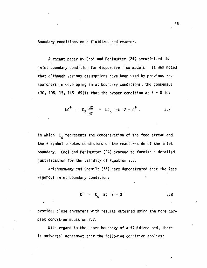
Boundary conditions on a fluidized bed reactor.

A recent paper by Choi and Perlmutter (24) scrutinized the

inlet boundary condition for dispersive flow models. It was noted

that although various assumptions have been used by previous re-

searchers in developing inlet boundary conditions, the consensus

(30, 105, 15, 145, 69)is that the proper condition at Z * 0 is;

UC+ - D7 4£ = UC at Z = 0+ . 3,7L dZ °

in which C represents the concentration of the feed stream andothe + symbol denotes conditions on the reactor-side of the inlet

boundary. Choi and Perlmutter (24) proceed to furnish a detailed

justification for the validity of Equation 3.7.

Krishnaswamy and Shemilt (73) have demonstrated that the less

rigorous inlet boundary condition:

C* = CQ at Z = 0+ 3.8

provides close agreement with results obtained using the more com-

plex condition Equation 3.7.

With regard to the upper boundary of a fluidized bed, there

is universal agreement that the following condition applies:

27

— = 0 at Z = HD 3.9dZ B

in which HB = expanded bed height,

3.2 Fluidization Mechanics - Biomass Holdup

For a given set of operating conditions, an analysis of the

mechanics of fluidization within a FBBR yields two critical pieces

of information, the equilibrium biofilm thickness and bed porosity.

This information can, in turn* be used to calculate biomass holdup

within the reactor.

The concentration of particles which can exist in a fluidized

bed reactor at steady-state is a function of particle-fluid velocity

and other physical parameters which characterize the system such as

particle surface, size, shape and density and fluid viscosity and

density. Many experimental and theoretical studies have attempted

to define a quantitative relationship linking these factors. The

most common approach is to first define a relative velocity - phys-

ical parameter correlation for an isolated particle; then extend

this isolated particle treatment to cover multiparticle systems

through inclusion of a correction factor dependent on bed voidage.

Therefore, the analysis of fluidization mechanics which follows

will begin with a treatment of the isolated particle case.

28

Consider the isolated particle shown in Figure 3.2, Under

conditions of dynamic equilibrium, the sum of the drag force on the

isolated particle FnT and the buoyancy force FD must equal the grav-Ul D

itational force FP. That is:b

FDI + FB ' FG ' 3'10

For a spherical particle these forces are defined as follows

niLU

2 2* dn pl UR Cn_ 2 _ L K u

TT Pi 9 dp

— 3.12

3.13

in which CQ = drag coefficient

Un = relative particle - liquid velocity.

The relationship among drag coefficient, relative velocity

and a system's physical parameters has been the subject of ex-

tensive study. The consensus of these investigations (36) is pre-

sented in Figure 3.3. When the physical parameters which describe

a system are known, Figure 3.3 can be used to calculate the equili-

brium relative velocity (UR = terminal velocity U.) of a particle by

Figure 3.2 Forces Acting on a Fluidized Particle

29

O

10000

1000

100

10

0.1

0.001

-J 1 1 1 I L.

0.1 10 100 1000 10000 10!

Re

Figure 3.3 Correlation of Drag Coefficient vs. Reynolds Numberfor a Single Solid Sphere (After Foust (36)) .

30

31

a trial and error procedure.

To avoid the tedium of a trail and error solution, Zenz (156)

has proposed that the following demensionless groups be correlated

(Re/CD)1/3 = U

(ps "3 P

-1/3

3.14

(Re2 CD)1/3 = dp

4gpL (PS - PL)

-1/3

3.15

Wallis (140) has termed these quantities the dimensionless

velocity and the dimensionless particle diameter, respectively. A

plot of dimensionless velocity versus dimensionless particle dia-

meter is reproduced in Figure 3.4.

For convenience in numerical calculation and particularly in

computer-aided solution, mathematical descriptions of the graphs

presented in Figures 3.3 or 3,4 are desirable.

In the Stokes' region of flow (approximately Re < 1) inertia!

forces are negligible. Therefore, an analytical solution of the

simplified Navier-Stokes equations is possible and yields the fol-

lowing relationship for drag force on an isolated particle (36):

FDI = 3nidPUR3.16

10'

10'

10-1

CO

oQ)cc

10-3

10-4

10-1 100 10

(Re2 C,)1/3

10*

Figure 3.4 (-} 1/3 vs. (Re Cn)1/3 for a Single Solid Sphere

\LD'

(After (10)).

32

33

Using this result. Equation 3,11 can be solved for drag coeffi-

cient. The resultant expression can be written in terms of Rey-

nolds number, as follows:

CD = 24/Re 3.17

In the Newton's law region of flow (approximately 700 < Re <

20,000), viscous forces are negligible. Drag coefficient in this

region is approximately constant and given by (36)

CD = 0.44 - 0.04 3.18

Several empirical CD - Re correlations have been proposed for

flow in the intermediate region between the Stokes and Newton regions

The following "very approximate" relationship has been cited by

Bird et al. (14):

CD = 18.5 / Re'6 . 3.19

For the entire regime of flow conditions, Dallavalle (28) has

suggested the following approximate CQ - Re correlation:

CD = (0.63 + 4.8 / Re) 2 . 3.20

34

For an isolated particle, one of the CD - Re correlations pre-

sented above can be used to develop an explicit expression linking

relative velocity (terminal velocity) to the physical parameters des-

cribing the system.

For a multiparticle system however, relative velocity-physical

parameter expressions must be modified to include the effects of

bed porosity. The brief review that follows presents such modifica-

tions, which cover the spectrum from theoretical to purely empirical

approaches.

Theoretical models of multiparticle systems.

Jackson (53) states that "...the motion of a system of particles

suspended in a fluid is completely determined by the initial state

of motion,, the initial thermal state, the boundary conditions, the

Navier-Stokes equations to be satisfied at each point of the fluid,

together with the corresponding continuity equations and energy equa-

tions, and the Newtonian equations of motion of each particle, to-

gether with the heat conduction equations in its interior...When

the system contains many particles, as in suspensions of engineering

interest, the problem is far too complicated to permit direct solution

when stated in these terms."

For practical purposes, therefore, all theoretical models at-

tempting to describe the mechanics of multiparticle systems are based

35

on solution of the Navier-Stokes equations under particular sets of

limiting assumptions. Simplifing assumptions commonly used include:

(i) limitation of analysis to the creeping flow region

(ii) zero slip velocity on only part of the solid surface

(iii) no collisions between particles

(iv) no aggregation of particles

(v) choice of a convenient spatial arrangement of the particles

The most important theoretical models have been summarized by

Barnea and Mizrahi (10). The models together with their limitations

are presented In Table 3.1. Note that only the cell models are appli-

cable beyond the range of creeping flow.

Semi-theoretical models of multiparticle systems.

Both theoretical and semi-theoretical models of multiparticle

systems are based on solution of the Navier-Stokes equations under

simplifing assumptions. Semi-theoretical models differ, however, in

that they contain one or more empirical contants.. Several of these

models (153, 87, 16) are based on the adaption of fixed bed formulae

to fluidized beds.

Brinkman (16), in studying pressure drop through packed towers,

combined the Navier-Stokes equations for creeping flow with Darcy's

Table 3.1 Mathematical models and techniques used in attempts at the theoretical calculation of dragforces in multiparticle systems (after Barnea and Mizrahi (10)).

Name of the Method Principle Limitations

Reflections

Point forcetechnique

Cell models

Multipolerepresentationtechnique

Iterative approximation techniquefor successive correction of theperturbation resulting from solidsurfaces

The disturbance produced by a sub-merged particle is replaced by apoint force

The Navier-Stokes equations aresolved within a fluid cell encasinga representative particle. Theratio of the cell/particle volumeis related to the suspension concen-tration

Each object is approximated by atruncated series of multilobulardisturbances. It has been claimedthat this converges more rapidlythan the reflection method, repre-sents the desired boundaries moreprecisely than the point forcetechnique, and may therefore beapplied for more concentrated sus-pensions

The solution converges only for rela-tively dilute suspensions

Only for extremely dilute suspensions

Different solutions may be obtainedwith different assumptions on cell con-figuration and boundary conditions

This has been applied only to a limitednumber of particles

37

law (itself a solution of a particular case of the Navier-Stokes

equations) and obtained the following expression for superficial

velocity U:

[ 0.75 /5 -- = 1 +1 0.75 (5 - 2e - 3eM| 3.21

in which U. is the terminal velocity of an isolated sphere. It

has been noted that this equation does not provide a good fit to

experimental data (10).

Several researchers (82, 92, 127) have suggested the adaption

of the Carman-Kozeny equation to fluidized beds. Loeffler and Ruth

(87) have modified the Carman equation so that it reduces to Stokes

law as porosity approaches unity:

3.22u/ut - 1 2K(1 - e)e £3

in which K is an empirical constant.

Other investigators (102, 47, 115, 148,75) have proposed the

use of an apparent suspension viscosity u in developing correla-

tions to describe the relationship among U, e and a system's physical

parameters. The following general relationship has been suggested

(10, 95):

38

3.23

in which K, and K« are empirical constants.

Empirical models of multiparticle systems.

A number of researchers including Hancock (43)> Steinour (l27)>

Lewis et al. (86), Lewis and Bowerman (85) and Richardson and Zaki

(114) hate suggested the use of a log-log plot of porosity versus

superficial velocity. For all but very dilute suspensions, a linear

relation has been observed and is described by the following expres-

sion (114):

U _ n— £ 3.24

in which U. = U. for sedimentation

log U. = log IL - dp/D for fluidization

D = column diameter

n = empirical bed expansion index.

39

By dimensional analysis, Richardson and Zaki (114) have shown

that, in general, the expansion index n is a function of an aspect

ratio dp/D and the particle terminal Reynolds number Ret> defined by

Re,t

However, at extreme values of Re. (Ref < .2 or Re, > 500), the ex-

pansion index becomes independent of terminal Reynolds number.

The following empirical correlations have been developed for

uniform spherical particles by Richardson and coworkers (113, 114):

n = 4.65 + 20 dp/D Ret < 0.2 3.25

n = (4.4 + 18 dp/D) Ret~°'03 0.2 < Ret < 1 3.26

n = (4.4 + 18 dp/D) Re^0*1 1 < Ret < 200 3.27

n = 4.4 Re^' 200 < Ret < 500 3.28

n = 2.4 Ret > 500 3.29

For the entire range of particle concentration, Barnea and Miz-

rahi (10) have assembled data from the literature to show that a

hyperbolic function more accurately describes the log U - log e re-

40

lationship. This confirms the observations of Happle (44) and

Adler and Happle 0) who have suggested that Equation 3.24, under-

estimates the mutual interference of particles in very dilute sys-

tems giving values of superfical velocity which are too high in this

region. However, for fluidized bed reactors of practical interest,

an adequate description of the bed expansion characteristics is pro-

vided by the linear expression, Equation 3.24.

An interesting approach to the mechanistic description of

particulate fluidization has been advanced by. Wen and Yu (147).

They consider the various forces acting on an isolated particle in

dynamic equilibrium; then adjust this analysis to describe fluidi-

zation through inclusion of a correction factor which accounts for

particle interactions within the fluidized bed. Thus, Equation 3.10

can be rewritten:

FD + FB = FG 3.30

in which FD is the drag force on a constituent particle within a

fluidized bed.

Wen an Yu (147) relate the multiparticle drag force FQ to the

familar isolated particle drag force FDI through use of a correction

factor dependent on bed porosity, e. This correction factor f(e) can

be written in terms of drag forces as follows:

3.31

41

Using this expression, the particle force balance, Equation 3.30,

may be rewritten as:

FDI + FB ' FG . 3'32

Substituting the individual force equations, Equations 3.11, 3.12

and 3.13, into the force balance equation, Equation 3.32, the fol-

lowing expression for correction factor is obtained:

4dp (p - P,) gf(e) = — 5 J= 3.33

\f

Drag coefficient can be linked to superficial velocity using

one of the methods discussed earlier for the isolated particle case.

Wen and Yu (147) used Equation 3.33 to calculate f(e) for their

own experimental data and also for data reported in the literature

(86, 114, 150)- The resultant f(e) values were plotted against the

corresponding observed bed porosities and a linear relationship was

found to exist. Wen and Yu suggest the following expression to cor-

relate this data:

f(e) = e"4-7 3.34

42

The data base for this correlation includes spherical particle

systems with the following ranges of characteristics:

15 < dp < 6350 microns

31.06 < p < 11.25 g/cm

0.818 < p. < 1.135 g/cm

1.0 < p < 15.01 cp

0.00244 < dp/D < 0.1

An expression which links bed porosity to superficial velocity

and the physical parameters of a system is obtained by combining

Equations 3.33 and 3.34.

It should be emphasized that all correlations presented thus

far are directly applicable only to systems comprised at particles

which are spherical or nearly so. The effect of particle shape on

bed expansion will now be considered.

43

Effect of particle shape on bed expansion characteristics.

The terminal velocity of a particle of any shape is given by

the following expression;

1/2

3.35ut •

"2 V pg (p s - P L ) "

CD PL sp

in which Vp and Sp are, respectively, the particle volume and pro-

jected area normal to flow. Note that CQ must be evaluated at the

proper sphericity, . Sphericity is defined as the ratio of the

surface area of a sphere of volume equal to that of the particle, to

the surface area of the particle (36).

McCabe and Smith (89) state that "A different CQ - Re rela-

tionship exists for each shape and orientation. The relation-

ship must in general be determined experimentally...". The effect

of sphericity on the empirical CQ - Re relationship is shown in

Figure 3.5.

Previous research efforts have demonstrated that the expansion

(or sedimentation) behavior of a bed of uniform, non-spherical part-

icles is also described by a linear log U - log e relationship such

as Equation 3.24 (148, 114, 149, 35). These studies note, however,

10000

1000

TOO

QO

10

1

0.1

0.001 0.1 10 100 1000 10000 10*

Re

Figure 3.5 Drag Coefficient as a Function of Reynolds Number and

Particle Sphericity $ (After Foust (36)).

44

45

that larger values of the expansion index n are associated with non-

spherical particles.

For particles with Ret > 500, Richardson and Zaki (114) found

that the expansion index can be expressed in terms of a shape factor,

KF, defined as follows:

3"ad.

in which da * the diameter of a sphere with the same surfaceaarea as the particle

d. = the diameter of a circle of the same area asD

that projected by the particle when lying in

its most stable position.

Richardson and Zaki (114) developed the following correlation for

non-spherical particles with Ret > 500:

n = 2.7 Kp°'16 3.37

For smaller, irregular particles, Whitmore (149) has reported n

in the ranqe 6.9 to 9.5.

In an interesting study by Edeline, Tesarik and Vostrcil (33)

46

on the fluidization of chemical and biological floes, it was found

that n = 10.5 for the "very irregular particles of aluminum

powder" and n = 12 to 27 for the biological floes.

The larger values of n observed for non-spherical particles

have been attributed to "immobile fluid trapped with the solids due

to particle aqglomeration, occlusion in surface irregularities or

simply increased volume of boundary layer relative to the particle

volume" (35). Fouda and Capes (35) note that as a result of this

trapped fluid, the particles have a larger effective diameter but

lower density. Thus, a fluidized bed with an apparent porosity based

on solids volume, defined as:

ea = (1 - C ) 3.38

actually has an effective porosity with respect to fluidized volume

which can be defined as:

ee = (1 - K1 Cv) . 3.39

where C1 is the solid volume fraction and K1 is the volume of solids

nlus immobilized fluid oer unit solid volume. Using the linear log

U - log e relationship, Eouation 3.24, the apparent expansion index,

n , can be linked to the effective expansion index, n as follows:

47

In en = n - - 3.409 e 1" *a

Since non-spherical particles have significant quantities of bound

water, K1 > 1 and e < ea; therefore, n, > n . A hypothetical re-e a a epresentation of this phenomenon is depicted in Figure 3.6.

Fouda and Capes (35) developed the following empirical correla-

tion for K' :

r -i' = |(d2/

dl> (S ) I0.284

3.41

in which d- = diameter to encircle an average particle in its most

stable position

d, = average particle diameter based on sieve analysis

S« = surface area of an average particle

S.j = surface area of a sphere of equivalent volume.

The fluidization behavior of a bed of non-spherical particles can

then be described by:

E = (1 - K'C)n , 3.42

ID

O

based oneffective porosity

x^ based on

apparent porosity

log e

Figure 3.6" Hypothetical expansion curves based on apparent

and effective porosities.

48

49

in which K1 Is calculated using Equation 3.41 and n is calculated

using apparent particle properties and the correlations developed by

Richardson and coworkers (113, 114), namely Equations 3.25 - 3.29.

3.3 Substrate Conversion by Biological Films

Microorganisms which mediate reactions of interest in the bio-

chemical process industries rarely exist as individual cells dispersed

in solution (99). Rather these microorganisms agglomerate to form

gelatinous aggregates of bacteria and extracellular material. . When

fixed to solid support surfaces, the aggregates are commonly referred

to as biological films or biofilms. Unsupported aggregates are re-

ferred to as biological floe particles.

Electron-microphotographs of biofilms taken by Jones et al. (66)

show 0.5 to 1.0 micron diameter cells spaced approximately 1 to 4

microns apart within a matrix of extracellular material. This struc-

ture is conceptually similar to that of a porous catalyst in that

both contain discrete reactive sites and inert diffusion zones.

For reaction to occur, reactant molecules must be transported from

bulk-solution to reactive sites within a biofilm. Because more than

one phase is involved, such reactions are referred to as hetero-

geneous.

Atkinson and Daoud (2) and LaMotta (76) have noted the analogy

between substrate utilization by biofilms and heterogeneous catalytic

50

reactions. For heterogeneous catalytic reactions, Smith (123) lists

the following sequence of steps for converting reactants to pro-

ducts :

1. Transport of reactants from the bulk-fluid to the fluid-

solid interface

2. Intraparticle transport of reactants into the catalyst

particle

3. Adsorption of reactants at interior sites of the catalyst

particle

4. Chemical reaction of adsorbed reactants to adsorbed products

5. Desorption of adsorbed products

6. Transport of products from interior sites to the outer sur-

face of the catalyst particle

7. Transport of products from the fluid-solid interface into the

bulk-fluid stream.

It is common practice to simplify this general sequence so that

only the most significant steps are included in subsequent analysis.

LaMotta (76) has suggested the following sequence of steps as adequate

for biofilm systems:

1. Transport of substrate (reactant) from the bulk-fluid to'the

fluid-biofilm interface (external mass transfer).

2. Transport of substrate within the biofilm (internal mass

transfer)

3. Substrate consumption reaction within the biofilm.

Smith's (123) steps 3 - 5 are lumped together to yield LaMotta's

(76) step 2. Smith's steps 6 and 7 are neglected by LaMotta who notes

that product concentration will not affect the irreversible reaction

rate unless allowed to build to such a level that poisoning occurs.

Note that LaMotta's steps 2 and 3 take place simultaneously, while

step 1. occurs in series with these steps.

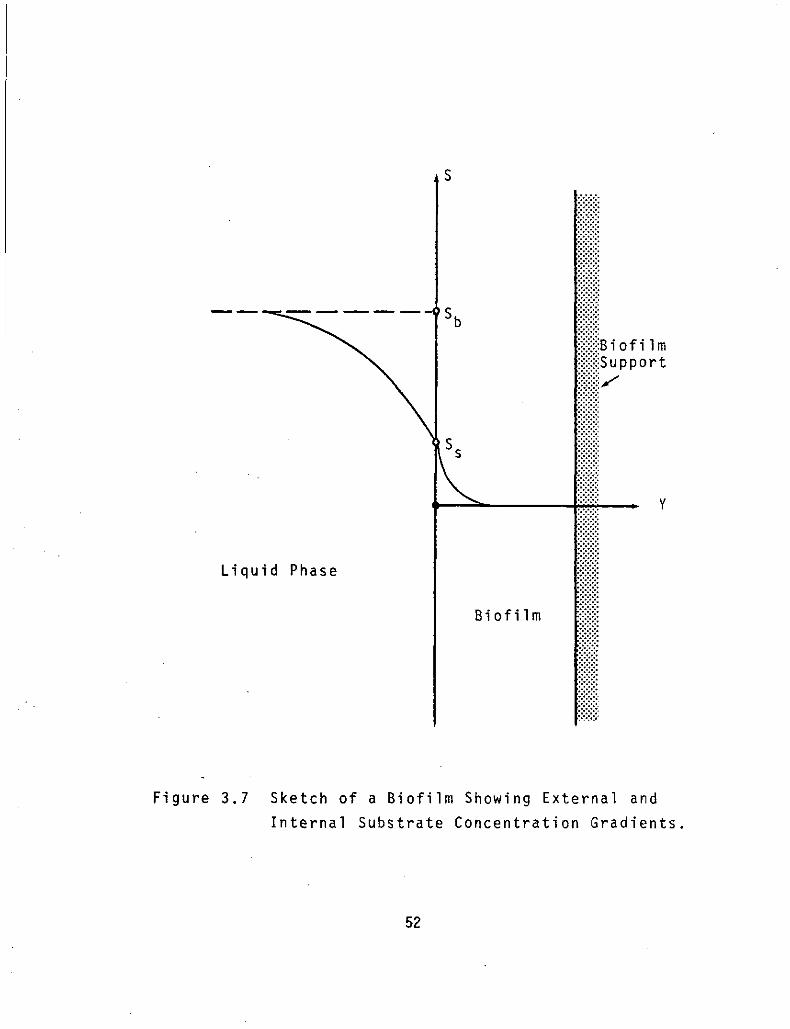
The mass transport resistances, delineated by steps 1 and'2, act

to establish concentration gradients within and around biofilms.

This situation is depicted in Figure 3.7. For intrinsic reaction

rates with a positive dependence on reactant concentration (Michaelis-

Menten, first order, etc.)» these gradients decrease the observed

rate of reaction by lowering local reactant concentration. For

intrinsic zero order kinetics, transport phenomena can decrease ob-

served reaction rate by limiting the depth of reactant pe'netration

within the biofilm.

3.3.1 External Mass Transfer

Fluid passing over a solid surface develops a boundary layer

which offers resistance to the transport of reactant molecules from

Liquid Phase

B i o f i 1 m

ijBiof ilm^Support

Figure 3.7 Sketch of a Biofilm Showing External and

Internal Substrate Concentration Gradients

53

the bulk-fluid to active sites on or within the solid.

A boundary layer is characterized by a drastic variation in

fluid velocity over a very small distance normal to the solid sur-

face. Satterfield (118) notes that "fluid velocity is zero at the

solid surface but anproaches the bulk-stream velocity at a plane not

far (usually less than a millimeter) from the surface."

In studying transport phenomena associated with biofilm systems,

Bunaay, Hhalen and Sanders (18) were able to experimentally verify

the existence of a concentration boundary layer at the biofilm-

liauid interface. Dissolved oxygen levels, measured with a micro-

orobe electrode, were observed to decrease sharply across a 100

micron liquid layer at the interface.

Many other researchers in the field of biological wastewater

treatment have considered the rate limiting effects of external mass

transfer resistance (76, 98, 8, 130, 88, 71, 4, 3, 2, 6, 68,

42, 18).

Because of the complex nature of flow near immersed objects, it

has been found necessary to develop semiempirical correlations, of

data on mass transfer between the chases (118). These data are com-

monly expressed in terms of an empirical mass transfer coefficient,

k .which "is related to the diffusional flux,N', at the solid surfaceU-

by the followinq relationship:

N' = kc (Sb - Ss) . 3.43

54

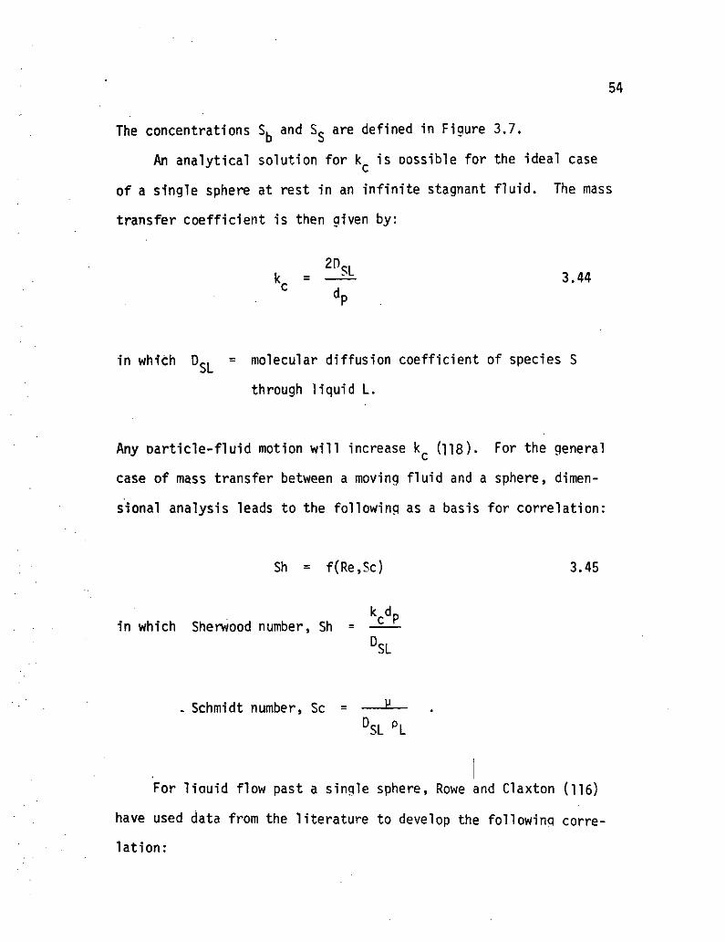
The concentrations S. and Sc are defined in Figure 3.7.D b

An analytical solution for k is oossible for the ideal caseL>

of a single sphere at rest in an infinite stagnant fluid. The mass

transfer coefficient is then given by:

2Dk = —^ 3.44C

in which D-, = molecular diffusion coefficient of species S

through liquid L.

Any particle-fluid motion will increase k (118). For tne generalL*

case of mass transfer between a moving fluid and a sphere, dimen-

sional analysis leads to the following as a basis for correlation:

Sh = f(Re,Sc) 3.45

kcdPin which Sherwood number, Sh = ——DSL

- Schmidt number, Sc =DSL PL

For liouid flow past a single sphere, Rowe and Claxton (116)

have used data from the literature to develop the following corre-

lation:

55

Sh = 2.0 + 0.76 :(Re)]/2 (Sc)1/3 3.46

This correlation applies to Reynolds numbers in the range 20 to

2000.

Under extreme flow conditions, liquid-solid mass transfer is

subject to analytical solution.

It has been noted (133) that for most systems of practical in-

terest, the characteristic Peclet number {Pe = dplL/D-.) of the

orocess is high (Pe > 1000). Restricting his analysis to this region,

levich (84) developed a solution for mass transfer to a single sphere

fallina throuah an infinite fluid. This solution can be expressed in

terms of the Sherwood number as:

Sh = 0.997(Pe)1/3 . 3.47

For spherical oarticles in Stokes flow (Re < 1), Friedlander

(37) developed the following approximate theoretical expression for

mass transfer:

Sh = 0.991(Pe)1/3 3.48

Tardos et al. (133) derived an expression for high Peclet

number mass transfer to a sphere situated in a swarm of like part-

icles. A porosity correction factor p(e) was introduced which accounts

56

for variations in velocity profile caused, by the particle swarm.

The correction factor is combined with the theoretical solution of

Levich, Equation 3.47, to yield the following expression:

Sh = g(e) • 0.997 (Pe)1/3 3.49

in which Peclet number is redefined in terms of superficial velocity

U as:

_ U dpPe = - 3.50

DSL .

Correlations which are directly applicable to interphase mass

transfer in fluidized beds are reviewed by Beek (12). Beek notes

that "a chaos of correlations, statements and conclusions is found

in the literature due to the fact that an increase in fluidization

velocity increases the bed expansion, which in-many cases is not

measured. The consequence is, that in the proposed correlations,

not only the influence of U (superficial velocity) on the fluid to

particle mass transfer coefficient k is hidden, but also that of

e (bed porosity) on k ."

Of the correlations discussed by Beek, the one proposed by

Snowdon and Turner (126) is of particular interest. This is due

to the fact that this correlation is based on data coverina a

57

similar Reynolds number range as that found in the FBBR. Snowdon

and Turner state that their experimental data are well correlated

by the following:

Sh = ^^- Re1'" Sc1/3

in which Reynolds number is defined in terms of superficial velocity

U as:

Up, dRe = L

Beek (12) developed a more general correlation of liquid-

particle mass transfer within a fluidized bed based on the data of

several researchers (126, 107, 112, 92, 25, 38), including Snowdon

and Turner. The correlation developed by Beek is as follows:

St • Sc2/3 = (0.81 * 0.05) Re~1/2 3.54

for 5 < Re < 500

in which Stanton number, St = k e/ U

This correlation results in slightly lower values of k than does\*

the correlation of Snowdon and Turner (126).

58

Although the correlation of Beek is founded on a broader data

base than that of Snowdon and Turner, the latter will be used in

subsequent sections of this dissertation to correlate k within a

fluidized bed biofilm reactor. This choice is made because of the

Reynolds number similarity mentioned earlier.

3.3.2 Internal Mass Transfer - FBBR

Internal mass transfer resistance acts to establish a con-

centration pradient within a biofilm. Thus, interior portions of

the biofilm are exposed to lower substrate concentrations than exist

in the bulk-fluid. This often results in observed reaction rates

which are significantly lower than would occur if mass transport

limitations were absent.

Analysis of this phenomenon is complex because internal mass

transfer and reaction occur simultaneously, therefore, neither pro-

cess can become limiting in the sense that it alone will determine

the overall or observed reaction rate (83, 76, 118, 51).

Among the first to report on the rate limiting aspects of inter-

nal mass transfer were researchers in the biomedical field. Krough

(74) in 1918, Warburg (141) in 1923, Fenn (34) in 1927, Hill (48)

in 1929, and Gerard (40) in 1931 all considered the effect of in-

ternal diffusion on oxygen utilization by respiring tissue or cells.

This early research is typified by the work of Harburg (141)

58

Although the correlation of Seek is founded on a broader data

base than that of Snowdon and Turner, the latter will be used in

subsequent sections of this dissertation to correlate KC within a

fluidized bed biofilm reactor. This choice is made because of the

Reynolds number similarity mentioned earlier.

3.3.2 Internal Mass Transfer - FBBR

Internal mass transfer resistance acts to establish a con-

centration pradient within a biofilm. Thus, interior portions of

the biofilm are exposed to lower substrate concentrations than exist

in the bulk-fluid. This often results in observed reaction rates

which are significantly lower than would occur if mass transport

limitations were absent.

Analysis of this phenomenon is complex because internal mass

transfer and reaction occur simultaneously, therefore, neither pro-

cess can become limiting in the sense that it alone will determine

the overall or observed reaction rate (83, 76, 118, 51).

Amonq the first to report on the rate limiting aspects of inter-

nal mass transfer were researchers in the biomedical field. Krough

(74) in 1918, Warburq (l4l) in 1923, Fenn (34) in 1927, Hill (48)

in 1929, and Gerard (40) in 1931 all considered the effect of in-

ternal diffusion on oxygen utilization by respiring tissue or cells.

This early research is typified by the work of Harburg (HI)

59

in which mass transfer, described by Pick's first law, and simul-

taneous zero order reaction are included in a mathematical des-

cription of oxygen utilization within muscle tissue slices. War-

burg's analysis allowed calculation of the "Grenzschnittdicke" or

limiting slice thickness such that just the center of the tissue

slice was anoxic.

The effect of transport phenomena on observed reaction rate

was next recognized by researchers in the field of heterogeneous

catalysis. Independently, Thiele (134), Damkohler (29) and Zeldo-

vitch (155) each developed quantitative descriptions of the factors

that determine a porous catalyst effectiveness. Catalyst effective-

ness was quantified by a parameter termed the effectiveness factor, n

Intraphase effectiveness factor can be defined as follows:

Observed

reaction

rate

Reaction rate which would occur if the

entire catalyst particle were exposed to

reactant of the same concentration as ex-

ists at the outside surface of the catalyst

Overall or interphase - intraphase effectiveness factor can be de-

fined as:

no

Observed

reaction

rate

60

Reaction rate which would occur if the

entire catalyst particle were exposed to

reactant of the same concentration as ex-

ists in the bulk-liquid.

In the absence of external mass transfer limitation, ny = n .

In the absence of all mass transfer limitations intrinsic kinetics

is observed with nT = *u = 1.I oSignificant mass transport limitations are associated with low

values of effectiveness factors. Kobayashi and Laidler (70) and

Satterfield (118) have suggested that ru = 0.95, and nj = 0.6

be used as criteria to indicate insignificant and significant internal

mass transfer limitations, respectively.

Thiele presented the results of his analysis as plots of ef-

fectiveness factor versus a dimensionless quantity, since termed

the Thiele modulus. This modulus lumps important system parameters

such as reactant concentration driving force, reaction rate constant,

effective diffusivity of reactant within the catalyst and catalyst

particle size.

Among the first researchers in the wastewater treatment field to

consider the effect of transport phenomena on observed substrate

utilization rate was Pasveer (104). He postulated that the inverse

relationship found to exist between observed rate and floe size was

61

due to oxyaen transport limitations within the floe particles.

Pasveer suggested intensification of turbulence within the aeration

basin as a means of increasing treatment efficiency through reduc-

tion of floe size.

In other research related to biological wastewater treatment,

Vluhrmann (154) used the theoretical analysis of Gerard (40) to

comoute the depth of penetration of oxygen in microbial aggregates.

Using an assumed effective diffusivity of 5 x 10" cm/sec and a

bulk-fluid oxygen concentration of 2 mg/1, Wuhrmann calculated that

the center of a spherical floe particle would just be respiring at

a critical oxygen tension of 0,1 mg/1 when the floe particle diameter

reached 500 microns. For fixed film systems with the same bulk-liquid

oxygen concentration, Wuhrmann estimated the critical biofilm thick-

ness to be 100 microns.

Mueller (98) examined mass transfer resistance related to the

utilization of oxygen by pure culture Zoogloea ramiqera floe

particles. It was demonstrated that at low dissolved oxygen concen-

trations, the overall rate of oxygen utilization was significantly

limited by internal mass transport resistances. The limiting dis-

solved oxygen levels for unblended floe particles were found to vary

between 0.6 and 2.5 mg/1 depending on temperature and floe size.

For blended floe samples, the resultant dispersed cells and smaller

floe particles exhibited markedly lower limiting dissolved oxygen

concentrations of 0.1 to 0.4 mg/1.

62

Mueller (98) developed an anoxic core model (zero order

kinetics) of a floe particle which was represented as a triangular

prism. Using this model, oxygen diffusivity within the floe part-

icle was determined to be about 8 percent of the corresponding value

in water.

Baillod and Boyle (9) examined the effects of glucose trans-

port within floe particles of Zoogloea ramigera on overall glucose

utilization rate. They concluded that glucose diffusion through the

floe matrix became rate limiting at low glucose concentrations. A

zero order anoxic core model was used to calculate the effective

diffusivity of glucose in the zoogloeal floe material. Calculated

effective diffusivities ranged from about 7 to 9 percent of the cor-

responding values for glucose in water.

Sanders (ll?) observed the effects of biofilm thickness on

film growth kinetics. Biofilm was allowed to develop on the inside

wall of a continuous flow culture chamber. Mixing of the chamber

contents was provided by a magnetic stirrer. A nutrient broth feed

solution was used.

Sanders postulated that biofilm organisms exist in either repro-

ductive or retarded stages of growth. He attributed retarded growth

to limiting levels of oxyaen or nutrients caused by diffusional re-

sistances. The thickness of the "active" reproductive stage is referred

to as the limiting film thickness.

63

Sanders observed that oxygen utilization rates increased with

film thickness until the limitina film thickness (21.2 microns) was

reached; beyond this point the rate of oxyqen utilization remained

constant.

Tomlinson and Snaddon (135) examined factors affecting the bio-

logical oxidation of sewage using an inclined rotating tube biofilm

reactor. It was observed that carbon removals increased with film

thickness until depths of approximately 120 microns were obtained.

Beyond that thickness, removals remained constant. The anoxic core

model developed by Warburg (141) was used to calculate the effective

diffusivity of oxygen within the biological film. The value ob-

tained was approximately 67 percent of the corresponding value in

water.

Maier (88) used an inclined plane biofilm reactor to examine

factors which affect the rate of glucose removal. Uniform biofilms

were obtained by containing the films within a screen framework.

Film thickness was controlled by scraping such that film thickness

corresoonded to screen thickness.

Maier observed that biofilm thickness had no effect on glucose

removal. He therefore concluded that "the thickness of the slime

layer is not an important variable." Baillod and Boyle (9) later

pointed out that the film thicknesses used by Maier (480-1400 microns)

were too great to allow observation of any change in uptake rate

with thickness.

64

Kornegay and Andrews (71) studied blofilm substrate utilization

kinetics usina annular reactors. The reactors consisted of en-

closed outer vessels which housed rotatinp drums. External mass

transfer resistances were minimized by rotating the drums at 100 rpm.

The substrate consisted of glucose and a mineral base. Dissolved

oxygen was maintained at levels which exceeded limiting concentrations

A mathematical model of substrate utilization was proposed

based on the hypothesis "that the entire mass of attached microorgan-

isms is not active in the removal of soluble organics" (71). Monod

(Michaelis-Menten) kinetics was used to describe the model reaction

term. Experimentally* Korneaay and Andrews (71) observed that sub-

strate removal rate increased linearly with film thickness until

the "active thickness" (80 microns) was exceeded. Greater film thick-

nesses resulted in no further increase in the rate of removal. A

Lineweaver-Burk plot was used to determine the biological kinetic

contants. The effect of internal mass transfer on such a plot was,

however, not considered resulting in an unreasonably large Michaelis

constant (K~ = 121 mg/1).

Atkinson and Daoud (3, 4) presented a theoretical analysis of

substrate utilization by biological films. Their analysis draws on

the analogy between biological reaction and heterogeneous catalysis.

Specifically, a differential equation was developed which describes

internal mass transfer of reactant and simultaneous biochemical

reaction. A Michaelis7Menten kinetic expression was used. The re-

65

sultant differential equation is identical to one developed by

Schneider and Mitschka (119) for transport and reaction (Langmuir-

Hinshelwood kinetics) within a porous catalyst. Atkinson and Oaoud

(4) present the numerical solution of Schneider and Mitschka for the

common differential equation.

Simplified solutions were also presented for asymptotic forms of

the differential equation. For thick films, Atkinson and Daoud's

asymptotic solution predicts that substrate uptake will by indepen-

dent of film thickness. This result agrees with phenomena observed

by previous researchers.

Bungay, VJhalen and Sanders (18) utilized a.microprobe electrode

to examine oxygen profiles near the interface and within biological

films. When low concentrations of substrate were fed to the biofilm

reactor, a flat, high concentration oxygen profile was observed

within the biofilm, indicating substrate limited respiration. More

concentrated substrate feed solutions caused a significant internal

oxygen gradient indicating oxygen limited respiration. The effective

diffusivity of oxygen within the biofilm was calculated assuming

zero order reaction kinetics. The resultant value was approximately

2 percent of the corresponding value in water.

Hoehn (49) examined the effects of thickness on the activity

of bacterial films. A horizontal rotating cylinder was used as the

growth support surface. A synthetic feed solution was used. Hoehn's

observations agreed with previous researchers in that substrate

66

utilization rate increased with film thickness until a limiting value

(100 microns) was reached. For thicker films a constant substrate

utilization rate was observed. Hoehn attributed the leveling off of

utilization rate to oxygen limitations within the biofilm imposed by

diffusional resistances.

LaMotta (76) evaluated the external and internal diffusional

resistances associated with substrate utilization by biological films.

An annular reactor, similar to that used by Kornegay and Andrews (7l)

was used in the experimental portion of this study. The reactors

differed, however, in that LaMotta held the inner drum stationary and

rotated the outer cylinder. A glucose feed solution was used. Oxygen

levels were maintained in excess of limiting concentrations.

LaMotta's experimental results were consistent with previous

studies in that substrate removal increased with film thickness un-

til a limiting thickness was reached. Beyond this limiting thick-

ness, removal remained constant. LaMotta demonstrated that the limit-

inp biofilm thickness increased with increased concentration of glucose

in the feed stream. A mathematical model was developed which con-

sidered internal mass transfer and simultaneous zero order reaction.

The average effective diffusivity of glucose within the biofilm was

calculated to be aoproximately 44 percent of the corresponding value

in water.

Williamson and McCarty (152) proposed a model of substrate

utilization by bacterial films. The model is basically the same as

67

the model proposed by Atkinson and Oaoud (3, 4). Both .pairs of

researchers describe substrate utilization as a process of mole-

cular diffusion and simultaneous biochemical reaction with Michaelis-

Menten (Monod) reaction kinetics.

The model of Williamson and McCarty is for a single rate-limiting

species. Criteria are presented which allow a priori determination

of whether rate is limited by electron donor or electron acceptor.

Biological rate constants were obtained using a suspended growth

reactor. It was assumed that the constants so obtained were unaf-

fected by diffusional limitations. However, recent study by Shieh

(121) demonstrated that, in fact, significant diffusional limitations

are possible in suspended growth reactors.

In Williamson and McCarty's investigation effective diffusivities

within biofilms were obtained using an experimental apparatus designed

especially for that purpose. An ersatz biofilm was created by fil-

tering dispersed bacteria onto a support filter. The biofilm was

made inactive by restricting a needed reactant. The species under

study was allowed to diffuse through the biofilm and its concentration

history recorded. This record was then used to calculate an effective

diffusivity. The resultant effective diffusivities for ammonia,

nitrite, nitrate and oxygen all were between 80 and 100 percent of

the corresponding values in water.

Harremoes (44) has reported on the significance of internal mass

transfer (pore diffusion) to filter denitrification. He arrives at

68

conclusions which are similar to those of LaMctta (76) and wel l known

by analogy to heterogeneous catalysis, namely, that zero-order

intrinsic kinetics result in zero-order observed kinetics only when

reactants fu l ly penetrate a b io f i lm. When a rectangular b io f i lm is

only partially penetrated, zero-order intr insic kinetics results in

half-order observed kinetics. Harremoes presents concentration pro-

files for fixed f i l m denitr if icat ion systems which substantiate

the half-order concept.

3.3.3 Substrate Conversion Reaction

Common rate expressions used to describe substrate conversion by

biological systems include Michaelis-Menten (Monod) kinetics, dis-

continuous linear kinetics and zero-order kinetics. Of these rate

expressions, Michaelis-Menten kinetics offers the most general des-

cription of substrate conversion. That is, the Michaelis-Menten ex-

pression is applicable over the entire range of substrate concen-

trations.

Several researchers (71, 151, 19, 39, 41, 64, 80, 81, 78) in

biological wastewater treatment and related fields have concluded that

the consumption of both electron donors and electron acceptors fol-

lows Michaelis-Menten kinetics. For suspended growth systems the

Michaelis-Menten rate expression can be mathematically formulated as

fol1ows:

69

R = -- 3.55

in which R - Substrate reaction rate, mol/l.sec

S = substrate concentration, mol/1

X = microbial concentration, mg/1

k = maximum substrate reaction rate, mol/mg-sec

KS = Michaelis or half-velocity constant, rcol/1.

Figure 3.8 is a graphical representation of Equation 3.57 which illus-

trates the meaning of the parameters k and KV

Discontinuous linear kinetics describes the asymptotic regions

of the hyperbolic MichaeHs-ffenten curve, for S < < K- the following

expression describes substrate conversion kinetics:

"R * k ' S X 3.56

in which k l = k/Rs

For S > x K- substrate conversion is described by the following

equation:

R = kX 3.57

Figure 3.8 Reaction Rate Versus Substrate Concentration for

Michaelis-Menten Kinetics.

70

R = kX

R = kSX

Figure 3.9 Reaction Rate Versus Substrate Concentration forDiscontinuous Linear Kinetics.

71

72

Figure 3.9 depicts discontinuous linear kinetics. Obviously, the

discontinuous linear approach is least accurate in the region of the

discontinuity.

Simple zero-order kinetics is among the earliest expressions used

to describe biological reaction rates. Stumm-ZoTlinger et a!. (129)

note that as early as 1892, zero-order kinetics was reoorted as ap-

plicable to the description of fermentation rates. These authors

also note that substrate concentration dependence observed with mixed

substrate-mixed population systems may in fact be due to superposition

of many individual zero-order reactions. This argument is substan-

tiated by the fact that several researchers have observed zero-order

kinetics when dealing with single substrates or cure cultures (98, 9,

76). Further, there is evidence that reaction rates which appear to

follow Michaelis-Menten kinetics may, in fact, be intrinsic zero-order

reactions limited by diffusional resistances. LaMotta (76) has

shown that a zero-order, transnort limited biofilm model orovides an

excellent fit to the data of Kornegay and Andrews (71), which these

authors had modeled with Michaelis-Menten kinetics (1C = 121 ma/1).

One should, however, be mindful of the caution noted by Leven-

spiel (83) regarding zero-order kinetics. Levenspiel states that

"as a rule reactions are of zero-order only in certain concentration

ranges. If the concentration is lowered far enough we usually find

that the reaction becomes concentration dependent."

In summary, it is noted that although simplified linear kinetic

73

expressions are often adequate In describing observed rates of re-

action, the Michaelis-Menten equation offers a-'more general kinetic

expression applicable over a broader range of substrate concentrations

3.3.4 Biological Denitrlfication

The biochemical reaction of interest in this research is denitri-

fication. Biological denitrification may be either assimilatory or

dissimilatory (138). Assimilatory denitrification involves the re-

duction of nitrate-nitrogen to ammonia which is subsequently utilized

by the microorganisms for cell synthesis. If ammonia is already pre-

sent, assimilatory reduction of nitrate need not occur to meet cell

growth requirements (137).

Dissimilatory denitrification is a process by which nitrate-nit-

rogen is reduced to a gaseous nitrogen species by heterotropnic micro-

organisms (i.e., microorganisms requiring an external organic carbon

source. The gaseous product is primarily elemental nitrogen, however,

trace' amounts of nitrous of nitric oxide may also be formed (120).

A large number of bacteria are capable of dissimilatory nitrate

reduction while a much smaller number appear capable of assimilatory

reduction (103), That is, many organisms which denitrify require an

external source of ammonia for cell synthesis.

Organisms able to assimilate nitrate include Neurospora, Achromo-

, Aspergillus, Lactobacillus, Escherichia coli and Azotobacter.

74

Those capable of dissimilatinq nitrate include Micrococcus, Pseudomonas,

Denitrobacillus, Spirillum, Bacillus and Achromobacter (103).

It has been established that aerobic respiration (using molecular

oxygen) and dissimilatory nitrate reduction are homologous processes

I.e., the same electron-transfer pathways are followed in both re-

actions (132, 52, 101). The processes differ, however, at the terminal

enzymes. For dissimilatory denitrification, a nitrate reductase re-

places the aerobic process cytochrome oxidase as the terminal enzyme

of the metabolic pathway (120).

Organisms which can utilize either oxygen or nitrate as terminal

hydrogen acceptors are termed facultative organisms. Although facul-

tative organisms have the capacity to obtain energy from both nitrate

and oxygen reduction, the aerobic process is favored as indicated by

the following: (a) generally microorganisms denitrify only under

anoxic conditions and the presence of oxygen prevents the formation

of nitrate-reducing enzymes, (b) cell yield is usually lower in bac-

teria dissimulating nitrate than in those grown aerobically (which may

result from a lower formation of adenosine triphosphate during oxida-

tion of carbohydrate by nitrate), and (c) even cells with active ni-

trate-reducing enzymes can readily use oxygen instead of nitrate as

the terminal hydrogen acceptor (103).

In assessing the effect of oxygen on bacterial denitrification,

a differentiation must be made between assimilatory and dissimila-

tory nitrate reduction. Although assimilatory nitrate reduction is

75

unaffected by the presence of oxygen, it is generally accepted that

oxygen completely inhibits dissimilatory denitrification. While

dissimilatory nitrate reduction has been observed in aerobic systems

(50, 124), this denitrification has been attributed to mass transport

limitations which result in portions of the biomass being anoxic and

thus able to reduce nitrate (103, 50, 122).

Other important factors affecting biological denitrification are

temperature, pH and carbon source. Dawson and Murphy (31) found that

for a pure culture of Pseudomonas denitrif Jeans, the dependence of

denitrification rate on temperature can be described by an Arrhenius

type relationship. Specifically, these researchers developed the*\

following correlation between zero-order rate constant k (mg NO^-N/mg

cells-hr) and temperature:

k = 3.19 exp - ' 3.58T(°K)

Similar dependence of denitrification rate on temperature has been

observed in mixed culture biological denitrification (TOO). Stensel

(128), however, found that the rate of denitrification at 30°C was the

same or less than the rate at 20°C. He did observe that an Arrhenius

expression fit his rate data over a temperature range of 15°C to 25°C.

The results of several researchers who examined the effects of pH

on biological denitrification are presented in Figure 3.10. These re-

sults indicate an optimum pH in the range of 6.5 to 7.5. In reviewing

literature denitrification data, Harremces and Riemer (4.4) note that

6.0 7.0PH

8.0 .9.0

Figure 3.10 Effect pH on Denitrification Rate (after (137))

76

77

optimum denitrification results when pH is between 7.0 and 8.2. Sig-

nificantly reduced rates were noted at pH 6.0.

As mentioned earlier, the heterogeneous microorganisms which medi-

ate dissimilatory denitrification require an external source of organic

carbon. The most common organic compound used in denitrification is

methanol. Other organic materials, ranging from sugar to brewery

wastewater, have been examined as substitutes for methanol in denitri-

fication (90, 9l). Although several of these compounds were found to

be satisfactory from a biokinetic standpoint, other problems such as

cost or availability were noted.

C H A P T E R I V

FLUIDIZED BED BIOFILM REACTOR - MODEL DEVELOPMENT

4.1 An Hverview of the Model

Reactor flow model.

The dispersion model will be used to describe flow conditions

in the fluidized bed biofilm reactor. Development of the disper-

sion model proceeds under the following assumptions:

1. The liquid phase moves through the reactor by convection

and axial dispersion.

2. Mo radial gradients exist.

3. Solid phase characteristics (film thickness, bed porosity)

are independent of axial position.

4. Substrate uptake is solely by biologically active fluidized

particles.

5. Steady-state conditions exist in the reactor.

A differential element within a FBBR is shown in Figure 4.1.

A material balance on the differential element for any reactant can

be written as follows:

78

leaving bybulk flow

Z + AZ

entering bybulk flow

leaving byaxial dispersion

entering byaxial dispersion

Figure 4.1 Differential Element Within a FBBR

79

80

(output-input) + (output-input) +bulk flow axial dispersion

disappearance + accumulation =0 4 .1by reaction

In terms of bulk-liquid substrate concentration Sfa the individual

components can be expressed as;

entering by bulk flow = UA-S.L

leavino by bulk flow = UA-S. L + z

dS.entering by axial dispersion = - D7A L

L dZ L

dS.leaving by axial dispersion = - D^A L _

dZ

disapperance by reaction = (- R ) A A Z

accumulation = 0 at steady-state.

where: U = sunerficial upflow velocity

A = reactor area perpendicular to flow

Z = axial coordinate

81

Dy = axial dispersion coefficient

R = reaction rate in terms of reactor volume,

(mass substrate reacting)

(time) (volume reactor)

Entering these terms in Equation 4.1 and dividing by A A Z yields:

AZ- D-

- dS (IS.b t Ilk idZ 'Z+AZ " dZ _'Z

AZ+ Ry = 0 4.2

Takinq the limit as AZ -»• 0, obtain

dS

dZ

d2S,

' D4.3

Boundary conditions for Equation 4.3 were discussed in Section 3.1 of

this dissertation. The following conditions will be used:

Sb = Sb'z * 0 at Z = 0 4.4

5dZ

= 0 at Z = H. 4.5

In dimensionless form Equation 4.3 may be written:

82

& - B. 44 +/ L__\ D = o 4.6

in which: B = Sb / S^I^Q

Y = Z / H B

HB - expanded bed height

T = HR / UD

BA = Bodenstein number =o

Dimensionless boundary conditions on Equation 4.6 are:

B = 1 at Y = 0 4.7

— = 0 at Y = 1 4.8dY

Reaction term.

The Michaelis-Menten rate expression discussed in Section 3.3.3,

will be used to describe intrinsic (not limited by transport pheno-

mena) reaction kinetics within the FBBR. For biofilm systems, in-

trinsic Michaelis-Menten kinetics may be written in terms of the

bulk-liquid substrate concentration S. as:

k PR S,R = £_£ 4.9

* \t m f*

83

in which: R = mass substrate reacting(time) (volume bio-film)

mass volatile solidsp _

volume biofilm

. - mass substrate reacting.(time)(mass volatile solids)

The observed (mass transfer limited) rate of reaction within

a FBBR can, in turn, be related to the intrinsic rate by an overall

effectiveness factor n , introduced in Section 3,3.2. The observed

rate R can be written as follows:

4.10

Details of the procedure used to evaluate n are presented in Section

4.3 of this dissertation.

Biomass holduo

At any point in a FBBR, the observed rate of reaction on a per

unit biofilm volume basis R is related to the reaction rate on a

per unit expanded bed volume basis R by the following simple expres-

sion:

84

R0lz ' V '

Rv'z

in which the biomass volume Vg is uniformly distributed in the expanded

bed volume HDA. The expanded bed reaction term R can be written inD r V

terms of the bulk-liquid substrate concentration S. by combining Equa-

tion 4.9, 4.10 and 4.11 as follows:

RHBA Ks + Sb

The biomass holduo (VB / HRA) can be determined using an analysis

of fluidization mechanics within the FBBR. Details of the procedure

used in this determination are given in Section 4.2.

Basically, the fluidization analysis allows prediction of the

equilibrium bed oorosity and biofilm thickness corresponding to a

given set of reactor operating conditions. Biomass holdup may, there-

fore, be conveniently expressed in terms of bed porosity e, and the

operating parameter, media volume V as:

VB - v* 4.13HBA HBA

85

Axial dispersion coefficient

The axial dispersion coefficient correlation developed by Chung

and Wen (26), Equation 3.5, was incorporated in the FBBR model.

3.5Re

Pefl = — = -!^ [o.20 + 0.011 Re'48]A L J

The Bodenstein number is then written:

Bo = dp / (HB ' PeA)

The minimum fluidization Reynolds number ReMF was calculated using

the following correlation, developed by Wen and Yu (147):

"MFF(33.7)2 + 0.0408 Ga 1 - 33.7 3.6

in which the Galileo number Ga is defined as follows

p. (p - p ) gS L —

2y

Comprehensive FBBR model.

Equations 4.12 and 4.13 were used to eliminate the reaction term

Ry from Equation 4.3. The resultant expression is:

rfc AQ5i_ Q JLu — - DZ-1TdZ L &T °

1 - e -HBA

k "B Sb

86

= 0 4.14

Equation 4.14 may be rewritten in terms of dimensionless quantities as:

dB D d2B ,- Bo - + nT k Pg

Sb Z=0

B

n + B= 0 4.15

in which: = KS /

Bioparticle effectiveness factor n is dependent on bulk-liquid

substrate concentration S. (or B). This necessitates simultaneous

solution of Equation 4.14 (or 4.15) with an equation which expresses

the functional dependence of nn on S.. Such an expression is devel-

oped in Section 4.3 of this dissertation.

Section 4.2 presents details of the procedure used to predict

bed porosity e and biofilm thickness 6 as functions of operating con-

ditions within a fluidized bed biofilm reactor.

4.2 Fluidization - Bed Porosity and Biofiln Thickness.

An algorithm has been developed for calculating the equili-

brium biofilm thickness 6 and bed porosity e which correspond to a

given set of FBBR operating conditions. At the core of this algorithm

is the empirical bed expansion expression, Equation 3.24, discussed

87

in Section 3.2 of this dissertation. The algorithm is- presented in

flow chart format in Figure 4.2.

Basically, the bed expansion corresponding to a trial bio-

film thickness 6 is calculated using the bed expansion expression

Equation 3.24. Iteration continues on 6 until the calculated ex-A

nanded bed height HB coincides with some specified bed height Hg.

In order to use Equation 3.24, two parameters specific to the

system must first be determined. These parameters are the particle

terminal velocity U. and the.expansion index, n. Correlations for

these parameters, specific to the fluidized bed biofilm reactor,

have been developed as part of this research (see Section 5.2 and

5.3).

A step by step description of the fluidization algorithm follows

1. Guess a biofilm thickness <S.

2. Calculate the diameter of the biofilm-support medium

composite particle (or bioparticle):

dp = dm + 2 6 4.16

in which d = support particle diameter.

3. Calculate the biofiln) volatile solids density and wet

density corresponding to 6. It has been reported in the

88Figure 4.2 Flow Chart of the Bed Fluidization Algorithm

m pm m

Figure 4.2 ( can ' t ) 89

Eq. 4.22

Ret

Eq, 4.23

Eq. 4.24

Eq. 4.25

HB

Eq. 4.26

Yes

6 = 5 +

Eq. 4.27

PRINT6 dp

e X

90

literature (49) that biofilm volatile solids density is a

function of biofilm thickness. A decrease in volatile solids

density with film thickness was observed in this research,

however, the decrease was apparent only for relatively thick

{($ > 300) biofilms. Volatile solids - biofilm thickness data

for the experimental FBBR are presented in Figure 5.13.

The biofilm density-biofilm thickness relationship is incor-

porated in the fluidization algorithm through simple linear

functions which roughly correlate the data of Figure 5.13-

The correlation equations are given as follows:

PB = 65 mg g'5 ' , 0 < 6 < 300 microns 4.17acm

- 9 300 < 6 < 630 microns 4.17b330 micron-cm / cm

p = 30 *' , 6 > 630 microns 4.17c8 cm3

Both biofilm volatile and total solids density were mea-

sured in the experimental phase of this research. The ratio

of volatile to total biofilm solids was found to be approxi-

mately constant at 0.8. Using this ratio, the biofilm wet

density can be calculated by the following approximate rela-

tionship:

91

PBW « PL + PB / 0.8 4.18

4. Calculate the composite wet density pc of the bioparticle:

"S - "BW + ('m- W (V V 4'19

in which p is the support media density.

5. Calculate the terminal velocity U. of the bioparticle. For

smooth, spherical particles, terminal velocity may be cal-

culated using Newton's law, Equation 4.20 (36):

4(pc - P, ) g dDPL

*

Equation 4.20 is applied here to the calculation, of ter-

minal velocities for the irregular bioparticles. The

effect of particle shape and surface on terminal velocity

is introduced through the CD - Re correlation:

CD = 36.66 Re"2/3 4.21

which has been developed specifically for bioparticles

as part of this research. The experimental basis for the

92

correlation is described in Section 5.3.

Equations 4.20 and 4.21 are combined to yield the

following explicit expression for bioparticle terminal

velocity:

p ) gH ' *__ _7 7 7 T 327.5 p ' y

6. Calculate the bioparticle terminal Reynolds number Ret

U. P, dpRe = JL-k-P 4.23

y

7. Calculate the expansion index n which corresponds to

this bioparticle terminal Reynolds number. The following

empirical correlation is used:

n = 10.35 Ret'°-18 4,24

This correlation is specific for bioparticle fluidization

and has been developed as part of this research. The ex-

perimentation backing this correlation is described in

Section 5.2 of this dissertation.

93

8. Specify a superficial velocity U.

9. Calculate the resultant equilibrium bed porosity e using

Equation 3.24 with U = U.

4.25

10. Specify the total volume of support media in the reactor V .

11. Calculate the resultant trial expanded bed height HB using

a volume balance on solids within the reactor:

vm / d p \ 3

HR = —5L_ *L 4.26B A (1-e) \ d m/

12. Compare the calculated bed height HR with the specified

bed height HR. If unacceptable, return to step 1 and re-

peat the procedure.

As an aside, biomass holdup (actually volatile solids con-

centration per unit expanded bed volume) X may be calculated

as follows:

X =A H B

H 3

4.27

94

4.3 Substrate Conversion - Biofilm Effectiveness

As presented in Section 3.3, the rate of substrate conversion by

biological film is controlled by three major processes.

1. Transport of substrate from the bulk-liquid to the liquid-

biofilm interface (external mass transfer).

2. Transport of substrate within the biofilm (internal mass

transfer).

3. Substrate consumption reaction within the biofilm.

Mathematical description of substrate uptake by biological film

proceeds under the following assumptions.

1. Homogeneous biofilm of uniform thickness.

2. Mass transfer described by Pick's first law.

3. Single-substrate biochemical reaction described by

Michaelis-Menten kinetics.

4. Steady-state conditions.

Consider the idealized bioparticle depicted in Figure 4.3.

Under the listed assumptions, a material balance on a differential

shell within the biofilm can be written as follows:

BIOFILMConcentration

Boundary Layer

SUPPORT MEDIUM

Figure 4.3 Schematic of Bioparticle,

95

96

(output-inout) + disappearance + accumulation = 0 4.28internal by reaction

mass transfer

In terms of local substrate concentration S the individual com-

ponents of Equation 4.28 may be expressed as:

Input by internalmass transfer

DSB r2 dS

dr /r + Ar

output by internal

mass transfer* DSB r

2 dSdr / r

disappearing by reaction =k P So ^ MR

(47T rd Ar) B

accumulation = 0 at steady-state

in which D™ is the effective diffusivity of the substrate in the'SB

biofilm.

Entering these terms in Equation 4.28 and dividing through by

47T Ar yields:

'SBd r / r + A r V d r / r

Ar- r_2 k PB S

= 0 4.29

97

Taking the limit as Ar -»> 0:

n ^ / 2 ds \ 9 k p SSB T r :r- - / Ms

dr ) r ~ = ° 4-30

The effect of external mass transport or the rate of substrate

conversion is included in this analysis through the boundary con-

dition at the liquid-biofilm interface.

As discussed in Section 3.3.1, flux across this boundary may

be expressed in terms of an empirical mass transfer coefficient kf:

N1 = -kc (Sb - S) at r * dp / 2 4.31

This flux can, in turn, be related to biofilm-side concentration

gradient at the interface as follows:

°SB 3- = kc (Sb - S) at r = d / 2 4.32

The procedure used to evaluate the mass transfer coefficient

k is outlined at the end of this section.

At the biofilm-support particle interface, a no-flux boundary

condition applies. Thus:

= 0 at r = d / Z 4.33

98

Equation 4.30 and the accompanying boundary conditions, Equa-

tions 4.32 and 4.33, may be expressed in dimensionless form as:

1

{X + 0 dX

dC

dX J* 0 4.34

Y + C

^ = Bi (1 - C) at X =dX

4.35

dC

dXat X = 0 4.36

in which:

C = S/S,

X = r/6 - dm/26

S b D SB

» a Thiele-type modulus

99

69 a modified Blot number.

DS8

Equation 4.30 or 4.34 may be integrated numerically to yield

the substrate concentration profile within a bioparticle. Details

of the numerical integration procedure are presented in Appendix 1

The biofilm substrate concentration profile can, in turn, be

integrated to yield observed reaction rate, RO, as follows:

dp/2/- k pn S

dr

4.37

Overall effectiveness factor, n , is obtained by combining Equations

4.9, 4.10 and 4.37 to yield the following expression:

dp/2

f ^J K +

dr 4.38

Iff

In dimensionless terms, Equation 4.38 may be written:

1r c

+ 5 + 1/3 J Y + C0

100

(x + 0 dx 4.39

Details of the procedure for numerical integration of Equation 4.39

are included in Appendix 1.

External mass transfer coefficient k

Integration of the biofilm substrate conservation expressions,

Equations 4.30 or 4.34 requires a knowledge of the external mass trans-

fer coefficient, k«. As pointed out in Section 3.3.1, this coeffi-

cient can be related to conditions existing within a fluidized bed

biofilm reactor by the expression proposed by Snowdon and Turner (126)

Sh = P , Ml teV2 SCV3 3.53

DSL

This correlation was developed for fluidized beds operating under

the same-Reynolds number range as is common to fluidized bed biofilm

reactors.

101

4.4 A Summary of the Model

Prediction of substrate conversion within a fluidized bed

biofilm reactor requires simultaneous solution of the reactor flow

equation, Equation 4.15 and the biofilm effectiveness equations,

Equationons 4.34 and 4.39.

Solution of these equations is possible, however, only after

the parameters bed porosity, e, and biofilm thickness, 6, have been

specified. An algorithm, described in Section 4.2, is proposed as a

means of predicting these parameters.

To predict substrate conversion within a FBBR using the mathema-

tical models developed thus far, a total of thirteen system parameters

and six empirical correlations must be specified.

The required parameters and correlations are presented in Table

4.1. .System parameters are subdivided into fixed parameters (not readily

controllable by a designer) and design parameters,

Figure 4.4 further subdivides the parameters and correlations

as inputs to the appropriate segments of the overall FBBR model.

Details of the numerical solution of the FBBR model are presented in

Appendix 2. A computer program for such a numerical solution is included

in this appendix.

102

Table 4.1. FBBR MODEL INPUT PARAMETERS AND CORRELATIONS

Fixed Parameters

Liquid Phase Parameters:

diffusivity of species S in the liquid, DSL

liquid density, PL

liquid viscosity, y

Biofilm Parameters:

diffusivity of species S in the biofilm, DSB

maximum rate constant, k

Michael is constant, K-

System Dependent Parameters:

inflow concentration of species S, Sblz=0

inflow rate, Q

Design Parameters

Reactor Parameters:

horizontal area, A

expanded bed height, Hn

Support Media Parameters:

media density, p

media diameter, dm

total volume of media, V,m

103

Table 4.1 (con't)

Empirical Correlations

1) Biofilm density - biofilm thickness correlation, Equation 4.17.

2) Drag coefficient - Reynolds number correlation, Equation 4.21.

3) Expansion Index - terminal Reynolds number correlation, Equation 4.24

4) External mass transfer coefficient correlation, Equation 3.53.

5) Axial dispersion coefficient correlation, Equation 3.5.

6) Minimum fluidization Reynolds number correlation, Equation 3.6.

- V P..'Design Parameters

Q» u» P.Fixed Parameters

'B - s, CD - Re, n - Re1

Correlations

HLA, dDesign ParametersQ, k, K, D, DFixed ParametersSh - e, Re, ScCorrelations

FluidizationModel

Section 4.2

dm'A

Design Parameters

Q, k, K,., Sh 7=n

Fixed Parameters

Bo - e, Re, ReMF, ReMF-Ga

Correlations

BiofilmModel

Equations 4.34 &

4.39

ReactorModel

Equation 4.15

Sb(2)

Figure 4.4 Block Diagram of the FBBR Model

C H A P T E R V

EXPERIMENTAL PROGRAM

The basic objectives of the experimental portion of this re-

search were:

1. To obtain parameters and correlations needed as input to

the FBBR mathematical model.

2. To obtain FBBR performance data which can be used to eval-

uate the mathematical model.

Input information derived in this chapter includes the nitrate-

biofi 1m effective diffusivity DSB and the intrinsic rate constants for

biofilm denitrification, k and K<-. These parameters were determined

using a rotating disk biofiltn reactor. In addition, expressions re-

lating biofilm density to biofilm thickness, drag coefficient to

Reynolds number and expansion index to terminal Reynolds number were

determined experimentally using a laboratory scale fluidized bed bio-

film reactor.

Fluidized bed experimentation included the measurement of nitrate-

nitrogen profiles through the laboratory reactor. These observed pro-

files were compared with nitrate profiles predicted by the mathematical

model.

105

5.1 Rotating Disk Reactor

Bio-film Intrinsic Rate Constants and Effective Dlffusivity

The reaction of Interest in this research was nitrate-limited

biofilm denitri fication. Intrinsic reaction kinetics were described

in terms of a Michaelis-Menten rate expression. The rate constants

apnropriate to nitrate-limited biofilm denitrification were deter-

mined using a bench-scale biofilm reactor.

5.1.1. Materials and Methods

The Biofilm Reactor. The prime concern in selecting an experimental

reactor was that the reactor allowed a clear differentiation among the

steos involved in heterogeneous reaction i.e., among external mass

transfer, internal mass transfer and simultaneous biochemical reaction

One of the first reactors used in the environmental engineering

area to study biofilm reaction kinetics was the inclined plane reac-

tor (130, 88, 6, 68, 18). Substrate was allowed to trickle down a

biofilm covered inclined plane and factors affecting substrate consump-

tion were investigated. La I-iotta (76) notes, however, that such reac-

tors are unsatisfactory for rigorous examination of biofilm reaction

kinetics because the thickness of the external diffusional boundary

layer varies along the length of the planar reactor. Specifically,

106

107

the thickness of this boundary layer starts at zero at the leading

edge of the plane and increases with the square root of distance

along the axis of flow. Chambre and Acrivos (22) have shown that at

the leading edge of the reactor reaction kinetics controls conversion;

at the end of the reactor external diffusion controls; while between

these extremes, conversion is influenced by both reaction kinetics and

diffusional limitations. Because of this variation in diffusional

resistance, a clear differentiation between the reaction and transport

steps is difficult. Another problem encountered with the inclined plane

reactor is a tendency to develop biofilm with non-uniform thickness.

Maier (88) and Atkinson and co-workers (2,6) tried to eliminate this

difficulty by developing biofilm within a support grid. The biofilm

thickness was controlled by manually scraping the surface of the grid.

This technique limited their studies to relatively thick biofilms.

More sophisticated biofilm reactors were used by Kornegay (71)

and La Motta (76) in their studies of biofilm kinetics. The reactors

were concentric cylinders with one fixed, the other capable of rotation.

Biofilm of uniform thickness developed on the cylinder walls. Ex-

ternal diffusional limitation was eliminated by high-speed rotation

of one of the cylinders. By measuring substrate removal rate as a

function of biofilm thickness the effect of internal diffusional resist-

ance was separated from intrinsic kinetics.

An experimental reactor configuration which allowed an even

clearer differentiation among heterogeneous reaction steps was the

108

rotating disk reactor (RDR) used by Gulevich (42) in his biofilm

study. A clearer differentiation among steps was possible because the

rotating disk provides a uniformly accessible surface for interphase

mass transfer. A mathematical description of this phenomenon is pro-

vided by Levich (84).

Because it offers a relatively simple, yet rigorous means for

examining factors affecting biofilm kinetics, the rotating disk reac-

tor was selected for use in this investigation.

A schematic of the plexiglass experimental RDR used in this study,

with appropriate dimensions, is presented in Figure 5.1. A photo-

graph of the experimental apparatus is given in Figure 5.2.

As dissolved oxygen concentration is a critical parameter in bio-

logical denitrification, DO within the rotating disk reactor was con-

tinuously monitored using a YSI DO meter and probe (models 54 and 5739,

respectively). The reactor was fitted with a cover to aid in main-

taining anoxic conditions. In addition, nitrogen gas was continuously

fed to the RDR to strip out trace amounts of dissolved oxygen which

entered with the liquid feed. This gas was vented through the disk

shaft bearing in the reactor cover, preventing backflow of atmospheric

oxygen through this opening. The RDR effluent line was looped to pro-

vide a liquid barrier against oxygen intrusion via this route.

A schematic of a growth support disk is shown in Figure 5.3;

again dimensions are indicated. To facilitate measurement of biofilm

thickness, each plexiglass disk was fitted with four removable slides.

Feed Solution

N2 Feed

Shaft to DC Motor

Biofilm SupportDisk

DO Probe

Reactor Effluent

Figure 5.1 Schematic of the Laboratory Rotating Disk Reactor(scale 1/2" = 1").

109

WGINAl COPY'V*W* 1J * -• T' i

;• •- <j'.' . ? V'.*rt"vw *-* *>—W- j • ;

/•— ^:CS;1H^

Fio.ure 5.2 Photograph, of the lahrratory rotatino disk reactor.

PLAN RemovableSUdes

L C 1/9 I'r 3 i/t

r1 •-( ! !_ — __ _ _ _| U

1 1

.AZ'. .:—/ r ' ~~r1 "-r

' .v

' 3/8"

PROFILE

Figure 5.3 Schematic of the rotating growth-support disk*

112

The slides, also of plexiglass, were machined so that they formed an

integral part of the disk surface. The disk was rotated by a Fisher

Stedi-Speed stirrer. The disk shaft passed through a ball bearing in

the reactor cover; a brass point bearing was used to seat the shaft at

the reactor floor.

Two Masterflex pumps were used to supply liquid feed to the

rotating disk reactor. The pump which supplied the bulk of the in-

flow fed nitrified effluentfrom one of the extended aeration units

(Davco Package Plant Model 6DA7S) of the University of Massachusetts

Wastewater Pilot Ple.nt. The other pump supplied methanol and sup-

plemental nitrate (NaN03). To insure that methanol did not limit the

biological process, weight ratios of at least 6:1 methanol to nitrate-

nitrogen were maintained at the reactor inlet. The discharge lines of

the two feed pumps were joined at a Y connector, the reactor was fed

the resultant mixture.

The extended aeration unit effluent was used as feed only after

attempts at sustaining denitrifying biofilm with various synthetic

substrates had failed. Synthetic substrates used by Moore and Schroeder

(96), Requa and Schroeder (110) and Stensel (128) were all tried without

'success. Biofilm grown originally on the disk using extended aeration

effluent as growth medium, sloughed off and was eventually replaced by

a milky, weak (sloughed easily) biofilm which did not denitrify. In

all cases, make-up water was activated carbon-filtered Amherst tap

113

water. In an attempt to encourage growth, the organic carbon source

was switched from methanol to glucose; again without success. To ex-

pedite this research effort, extended aeration unit effluent with

methanol and supplemental nitrate added was used as feed during the

kinetic experimentation. Vigorous denitrifying biofilm development

resulted.

Next, problems with non-uniform growth were encountered when

disks were stored for long periods of time (more than a day) in a

horizontal position, as was the case in the RDR. Specifically, it was

noted that significantly thinner biofilm developed on the underside

of the disk. To eliminate differences in biofilm thickness between

disk surfaces, disks were stored, in a vertical position, outside the

RDR between experimental runs. The FBBR feed vessel-clarifier, de-

picted in Figure 5.10,offered a convenient location for vertical disk

storage. Since extended aeration effluent, methanol and nitrate were

also fed to this unit, the environmental conditions which existed there

were similar to those in the RDR.

Experimental Procedure. For all experimentation, volumetric flowrate3

into the RDR was controlled at approximately 50 cm /min. The volumetric

composition of the inflow was maintained, throughout, at an approxi-

mate ratio of ten parts extended aeration effluent to one part methanol

-nitrate solution. Determination of Michaelis-Menten coefficients

114

required that reaction rates corresponding to a range of substrate

concentrations be obtained. Therefore, nitrate-nitrogen feed con-

centrations of approximately 25, 50 and TOO mg/1 were used in the

RDR experimentation. Feed concentration was varied by changing the

concentration of the methanol-nitrate feed solution.

An experimental run was initiated by filling a clean (no wall

growth) reactor with a ten-to-one mixture of extended aeration ef-

fluent and methanol-nitrate solution. Nitrogen gas was then fed to

the reactor at a relatively high rate to eliminate any oxygen conta-

mination incurred during the filling operation. A biofilm covered

disk was removed from the FBBR feed vessel-clarifier and its edge

scraped so that only horizontal disk surfaces were biofilm covered.

The biofilm was gently rinsed with extended aeration effluent to

remove any loosely bound material. The disk was then placed in the

reactor and the reactor covered. The reactor was again purged of

oxygen by a brief high rate injection of nitrogen gas. When the DO

meter indicated that anoxic conditions had been achieved, the gas

flow rate was adjusted to the minimum level needed to maintain those

conditions.

Inflow pumps were then turned on and adjusted to yield desired

inflow rates and concentrations. Because nitrate levels in the ex-

tended aeration unit effluent were subject to fluctuation, inflow

nitrate concentration to the RDR was monitored during operation by

means of an Orion nitrate electrode (Model 92-07). It was observed

115

that for most runs, little or no variation in nitrate concentration

occurred over the 3 or 4 hour period of experimentation. When the

magnitude of variation did exceed 5 percent of the total nitrate

conversion across the reactor, the data were discarded.

A Fisher Stedi-Speed stirrer was used to rotate the biofilm

covered disk. Disk rotation was used as a means of eliminating ex-

ternal mass transfer limitation on observed reaction rate. In pre-

liminary experimentation, it was determined that external transport

effects were negligible for rotational speeds in the neighborhood

of 150 rpm. The experimental backing for this is given in Section

5.1.3. Disk rotation was controlled at 150 rpm for subsequent experi-

mentation.

The rotating disk reactor was operated, as described above,

until steady-state was achieved. To determine when steady-state

conditions had been attained within the RDR, reactor effluent ni-

trate concentration was measured intermittently. When no significant

variation in concentration was observed between successive samples,

the reactor was assumed to be at steady-state. Steady-state was

normally realized in 3 to 5 reactor detention times.

In addition to nitrate concentration measurement, the DO, pH

and temperature of the RDR contents were monitored during experimen-

tation. Anoxic conditions were maintained within the reactor through

control of the nitrogen gas flow rate. Although no direct control

116

was exercised over reactor pH and temperature, both parameters were

observed to be approximately constant at values of 6.9 ± 0.1 and

22°C ± 1°C, respectively, during experimentation. Because rate kinetics

are particularly sensitive to temperature, data were discarded when temp-

erature variation during an experimental run exceeded 1 C.

To account for any nitrate conversion within the reactor, not

attributable to the disk biofilm, a preliminary study was conducted in

which the RDR was operated both with, and without, the growth-covered

disk. After the RDR with disk had attained steady state, the disk

was removed and the reactor allowed to again reach steady state. It

was found that no nitrate reduction took place in the diskless reactor.

It was, therefore assumed in subsequent experimentation, that all

nitrate reduction observed in the RDR was due to the disk-supported

biofilm.

In order to measure the thickness of biofilm developed on the

disk surfaces, samples were taken by means of the removable slides

previously mentioned. The film thickness was then measured using ai

microscope equipped with a stage micrometer. The procedure used

is described as follows. A pencil mark was made on the slide sur-

face (i.e., at the bottom of the biofilm}. A mark was also made on

a sliver of cover glass (approximately 1 x 5 mm). The cover glass

was then placed mark down, crosswise, over the mark on the slide.

The microscope was focused first on the slide mark, then on the cover

glass mark. The difference in the micrometer readings provided the

117

thickness of the biofilm plus the marks. To correct for the thick-

ness of the marks, the procedure was repeated on a bare portion of

the slide; the thickness of the pencil marks was subtracted from the

total thickness measured to yield the net biofilm thickness.

At least five measurements of biofilm thickness were made on

each slide. For the relatively thin biofilms used in this study

(<5 < 350 microns) good film uniformity was observed, with the thick-

ness usually varying less than 10 percent across the length of the

slide. The ROR study was limited to these thin biofilms because of

sloughing problems encountered for thicker biofilms under the tur-

bulent conditions caused by disk rotation.

In addition to its thickness,the biofilm total and volatile

solids content were also determined. This was accomplished by per-

forming the appropriate analyses on a measured volume of biofilm which

had been scraped from the disk surface.

5.1.2 Theoretical Analysis.

A theoretical analysis of substrate conversion by biofilm pro-

vides the basis for the determination of nitrate-biofilm effective dif-

fusivity. This analysis is also useful for assessing the effect of

variation in parameters such as bulk-liquid substrate concentration

or biofilm thickness on substrate conversion rate.

118

Consider the differential biofilm element shown in Figure 5.4.

A general substrate mass balance was given earlier by Equation 4.28.

Specific terms for this balance equation, which apply to the RDR bio

film, are as follows:

mass entering by

intraphase transport1/2

dS

dY

mass leaving by

intraphase transport

1/2 dS_

dY Y + AY

- 1/2 A,- AYmass disappearing

by reaction

In which A = total biofilm surface area

accumulation 0 ' at steady-state.

Entering these terms in Equation 4.28 and dividing by 1/2 AT AY yields

'SB

dS

dY

dS

Y+ AY dY Y

AY

k PB s

KS + S= 0 5.1

Taking the limit as AY -> 0 gives

SB = 0 5.2

Bulk Solution

Flux in

Flux out

Figure 5.4 Differential Biofilm Element,

Biofilm

119

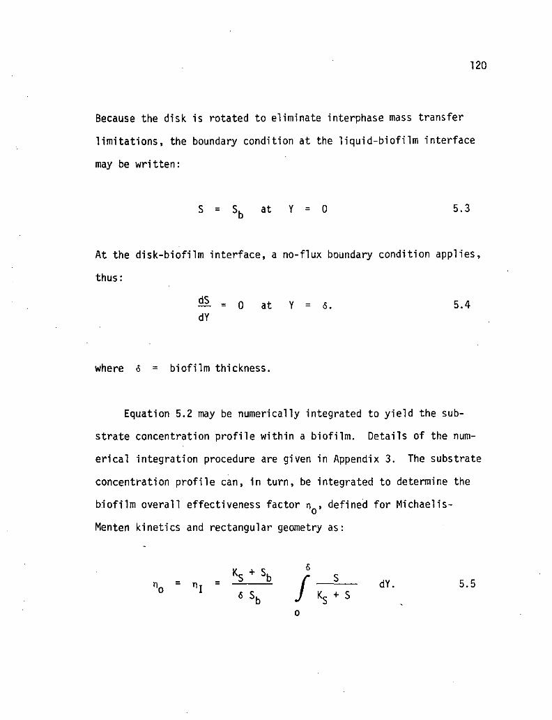
120

Because the disk is rotated to eliminate interphase mass transfer

limitations, the boundary condition at the liquid-biofilm interface

may be written:

S = Sb at Y = 0 5.3

At the disk-biofilm interface, a no-flux boundary condition applies,

thus:

^ = 0 at Y = 6. 5.4dY

where 6 = biofilm thickness.

Equation 5.2 may be numerically integrated to yield the sub-

strate concentration profile within a biofilm. Details of the num-

erical integration procedure are given in Appendix 3. The substrate

concentration profile can, in turn, be integrated to determine the

biofilm overall effectiveness factor n > defined for Michaelis-o

Menten kinetics and rectangular geometry as:

c

f-±J K +

dY. 5.56 S b

121

Details of the procedure for numerical integration of Equation 5.5

are included in Appendix 3.

If the intrinsic Michaelis-Menten parameters k and KS are known,

Equations 5.2 and 5.5 can be used to calculate the effective diffusivity

corresponding to an observed rate of reaction. The procedure used in

this calculation is outlined below.

Under steady-state conditions, a substrate mass balance on the

ROR may be written as follows:

Q (Sf - Sb) - AT 6 RQ 5.6

in which Q = volumetric flow rate

Sf = substrate feed concentration

R = observed rate of reaction.o

For kinetics described by the Michael is-Menten rate expression, Equa-

tion 5.6 may be combined with Equation 4.9 and 4.10 to yield the

following expression:

Q (Sf - Sh) - Ay 6 n - 2-2- = 0 5.7r b ' ° Kc + S.b b

Equation 5,7 is rearranged so that the overall effectiveness factor n

may be written in terms of observable quantities.

122

Q (Sf - Sb) (Ks H- Sb)n. ~ ~~~

0 A^ 6 P. k

For a given RDR experimental run, all quantities to the right of

the equality in Equation 5.8 are either measured or known; therefore

n can be calculated. The effective diffusivity for the given run may

be calculated:as follows:

1. Calculate r\ using Equation 5.8f-

2. Assume a trial value for effectiveness diffusivity, DSBA

3. Calculate a trial effectiveness factor n by numerical in-

tegration of Equation 5.2 and 5.5 using:^

(a) trial effective diffusivity, D-B.

(b) known Michaelis-Menten parameters, k and K~.

(c) measured bulk-liquid substrate concentration, S, , and

measured biofilm thickness, 6.

4. Compare the trial effectiveness factor (step 3) with the

observed effectiveness factor (step 1). If unacceptable, re-

turn to step 2 and repeat the procedure.

If a system's intrinsic Michaelis-Menten parameters and effective

diffusivity are known, Equation 5.2 and 5.5 can be used to predict sub-

strate conversion in the RDR. For a given set of operating conditions,

Q and S-, if the disk biofilm thickness is known, the reactor effluent

123

concentration, S,, can be calculated by an iterative procedure as

follows.

1. Specify: Biofilm parameters k, K~, DSB» PB,

operational parameters Q, So, A-..;

biofilm thickness 6.

2. Assume a trial bulk-liquid (i.e., effluent) substrate con-f*>

centration S, .b^

3. Calculate a trial biofilm effectiveness factor nQ by usingA

S, in the reactor substrate balance expression, Equation 5.8,

4. Calculate an independent (of step 3) trial biofilm effective-

ness factor rj by numerical solution of Equation 5.2 and 5.5

i.e., by a substrate mass balance on the biofilm.

5. Compare the effectiveness factors determined in steps 3 and

4. If unacceptable return to step 2.

6. Calculate substrate conversion Xc in the RDR as:

Xr - .- - 5.9c

5.1.3 Results and Discussion

Michaelis-Menten Constants. A substrate mass balance on the rotating

disk reactor resulted in Equation 5.2. Equation 5.2 as presented,

124

however, is not well suited for estimation of the Michaelis-Menten

rate constants k and K-. For this purpose it is useful to rearrange

Equation 5.2 to the Lineweaver-Burk format as:

*TKs

Q (S- - S. ) n k Sb nik 5.10M f b o °

To evaluate the intrinsic Michaelis-Menten coefficients, it is

necessary that external and internal diffusional limitations be elimin-

ated, i.e., that the overall effectiveness factor, nQ> be unity. Ex-

ternal diffusional limitation can be controlled by rotation of the

biofilm support disk. The rotational speed required to eliminate ex-

ternal diffusional limitation is determined experimentally by holding

all conditions constant within a RDR except disk rotational speed.

When an increase in rotational speed does not result in an increase

in substrate conversion rate, external diffusional limitation has

been eliminated.

Using a rotating disk reactor identical to that used in this study,

LaMotta (77) examined the effect of disk rotational speed on substrate

conversion rate. The results of LaMotta's study, shown in Figure 5.5,

indicate that external mass transfer limitation is appreciable for

rotational speeds under 70 rpm. To verify these results, the effect

of rotational speed on substrate conversion rate was examined as part

of this research. The results of this study are also shown in Figure

<D•Pfdoi

3e

•r—X(0

O•r—•M

LaMotta (77)

This Study

30 60 90 120Disk Rotational Speed (rpm)

150 01

Figure 5.5 The Effect of Disk Rotational Speed on ExternalMass Transfer Limitations.

126

5.5. Raw data for this experimentation is included in Appendix 4.

Based on the information presented in Figure 5.5 it was concluded

that external mass transfer limitations are negligible when disk rota-

tional speed is in the 150 rpm range. Rotational speed was controlled

at 150 rpm for subsequent experimentation.

To evaluate internal diffusional resistance, researchers in the

field of heterogeneous catalysis commonly reduce the size or thick-

ness of a catalyst and observe the effect of this reduction on ob-

served rate. When a decrease in catalyst dimension is not accompanied

by an increase in observed rate, it is assumed that internal mass

transfer resistance is negligible and that the observed rate is, in

fact, intrinsic.

A similar approach was used in this research. For a given set

of operating conditions, the effect of biofilm thickness on observed

reaction rate was examined. When a decrease in biofilm thickness was

not accompanied by an increase in reaction rate, it was assumed that

the kinetics observed were intrinsic.

To obtain the intrinsic data necessary to construct a Lineweaver-

Burk plot, reaction rates corresponding to a range of bulk-liquid sub-

strate concentrations must be determined. Toward this end, RDR-feed

concentrations of approximately 25, 50 and 100 mg/1 NO, - N were used.

For each feed concentration, experimental runs were conducted at various

,7

,6

.5

i/>

I A

<*-00

.2

cdG.

.1

0

36-310

microns

. 308

21O0

2700

44-177

microns

315

0130

2550

'155

-tr38

microns

Note:

Numbers next to experimentalpoints correspond to f^lm thick-ness in microns.

.01 ,02 ,03 ,04 ,05l/Sb {1/mg)

Figure 5.6. Lineweaver-Burk Plot of the RDR Data.

,06 t07

,8

CO>-<co

.6

.5JD

t/1

CO.4

COa.

.3

.2

,02 ,03 ,04

l/Sk

,05 ,06 07

ro03

Figure 5.7. Lineweaver-Burk Plot of the Intrinsic RDR Data.

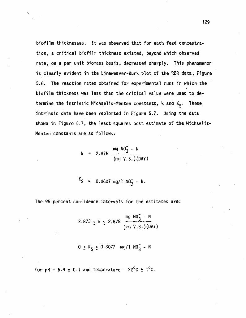
129

biofilm thicknesses. It was observed that for each feed concentra-

tion, a critical biofilm thickness existed, beyond which observed

rate, on a per unit biomass basis, decreased sharply. This phenomenon

is clearly evident in the Lineweaver-Burk. plot of the RDR data, Figure

5.6. The reaction rates obtained for experimental runs in which the

biofilm thickness was less than the critical value were used to de-

termine the intrinsic Michaelis-Menten constants, k and K~. These

intrinsic data have been replotted in Figure 5.7. Using the data

shown in Figure 5.7, the least squares best estimate of the Michaelis-

Menten constants are as follows:

mg NOl - N= 2.875 =

(mg V.S.MDAY)

= 0.0607 mg/1 NO^ - N.

The 95 percent confidence intervals for the estimates are;

mg NO - N2.873 < k < 2.878

(mg V.S.)(DAY)

Q < Ks < 0.3077 mg/1 NO" -

for pH = 6.9 ± 0.1 and temperature = 22°C ± 1°C.

130

Effective Diffusivlty. Having obtained the Michaelis-Menten constants

k and KS, the RDRdata were analyzed using the theoretical approach for

effective diffusivity presented in Section 5.1.2. This analysis

yielded a value for effective diffusivity for each of the RDR experi-

mental runs. The resultant 95 percent confidence internal estimate

for the mean nitrate effective diffusivity in biofilm is:

DCD = (0.815 ± 0.617) x 10"5 cm2/sec

OD

for T = 22°C ± 1°C.

This value is approximately 50 percent of the diffusivity of nitrate in

an aqueous solution at the same temperature (106).

The values of DSB, k and K- obtained for denitrifying biofilm were

used as input data to the theoretical analysis for substrate conversion

by biofilm presented in Section 5.1.2. For a given feed substrate con-

centration, biofilm thickness was specified and the resultant effluent

concentration and substrate conversion rate were calculated. By vary-

ing biofilm thickness and repeating the theoretical analysis, the

solid curves shown on Figure 5.6 were generated. These theoretical

curves provide a good fit to the observed data.

It is of interest to compare the rate constants with denitrifi-

cation constants reported in the literature. Table 5.1 presents

zero-order rate constants (approximately equal to the parameter, k,

Table 5,1 Literature Zero Order Den1trificat1on Rate Data,

Organismi

Micrococcus denitrificansMicrococcus denitrificansActivated SludgeActivated SludgeSpirillum (Undula?)Activated SludgeActivated Sludge

Activated SludgePseudomonas denitrificans

BiofilmBiofilm

Temperature°C

3732

20

20

25

20

8

11

25

20

5

20

27

27

25

Zero Order Denitrification RateData mg NO^ - N/(mg V.S.KDAY)

1,421,34,02-. 03

,01-22

2,88

,85

,03

. 02-34,33 ,58

,04,32-42

1.57-1.723,94-4,32

.05-1,3

.21-.31

Reference

23108

32659496

100

11

31

124

no

132

used in this research) reported by various investigators of bio-

logical denitrificat.ion. The low values reported for denitrifica-

tion with activated sludge can be attributed to the fact that only

a fraction of the biomass measured as volatile solids are actually

active in denitrification. The low values reported for biofilm

denitrification rate are likely the result of diffusional limitation

which mask intrinsic kinetics.

133

5,2 Fluidized Bed Biofilm Reactor - Bed Expansion

The purpose of the bed expansion study was to develop a

correlation for expansion index,n, applicable to the FBBR. Basically,

this experimentation involved varying the superficial velocity through

the laboratory FBBR and observing the effect of this variation on bed

porosity for an range of film thicknesses. The expansion index n

corresponding to a given biofilm thickness (more specifically to a

given terminal Reynolds number) was obtained as the slope of the re-

sulting log U - log e plot. Background information for this study

was given in Sections 3.2 and 4.2.

5.2.1 Materials and Methods

The Experimental FBBR. A schematic of the laboratory FBBR is given in

Figure 5.8. A photograph of the apparatus is shown in Figure 5.9. The

reactor was fabricated from 3.8 cm I.D. plexiglass column. Screened

sampling .plots were provided along the column length which allowed ex-

clusion of gross reactor solids from liquid samples. Separate sam-

pling poets were provided for solids removal. Approximately 12 cm of

pea gravel was used at the reactor inlet to provide even flow dis-

tribution and prevent backflow of support media.

A Masterflex pump was used to deliver feed solution to the FBBR.

3.8 cm

lo'cm

1

open sampling ports

T=117 cm_L

overflow

60 cm

1screened sampling ports

T21.5 cm

#L I<:•:< — _L-

inflow

Figure 5.8 Schematic of the laboratory FBBR,

134

135

COPV

.i .:<*

'IN

-v-

:.

Figure. 5.9 Plrotorpcapb. of the laboratory FBBR

136

The reactor feed consisted of clarified effluent from an extended

aeration unit at the University of Massachusetts Wastewater Pilot

Plant; methanol and supplemental nitrate (NaNO^) were added. To. in-o

sure that methanol did not limit the biological process, weight

ratios of at least 6:l,methano1 to nitrate-nitrogen were supplied.

As was the case with the RDR, the mixture of extended aeration unit

effluent and methanol nitrate solution was used as feed to the FBBR

only after attempts at sustaining denitrifying biofilm on various

synthetic substrates (see Section 5.1) had failed. The extended

aeration unit effluent was pumped into the pilot plant building by

a centrifugal pump situated over the extended aeration unit clarifier.

This pump delivered effluent to a feed vessel (a 750 ml flask) housed

in the FBBR clarifier as depicted in Figure 5.10. The solution of3

methane! and nitrate was pumped at a rate of approximately 5 cm /min

to the feed vessel by a Masterflex pump. The intake of the FBBR feed

pump was also located in the feed vessel (hence its name). Because

the inflow rate to the feed vessel was at least 50 percent greater

than the outflow rate due to the FBBR feed pump, the contents of the

feed vessel were not diluted by the bulk-clarifier contents. However,

in the event that extended aeration unit effluent flow to the feed

vessel was interrupted, the FBBR would continue to operate in a closed

loop with the bulk-clarifier contents supplying the feed vessel.

The biofilm growth support media used in this study were 25-30

mesh (590-710 micron) spherical glass microbeads.

to FBBR

from FBBR

12 in width

12 infeed vessel,(750 ml flask)

12 in

extended aerationunit effluent

methane! andnitrate solution

overf1ow

8 in

6 in

to drain

Figure 5.10 FBBR feed vessel and clarifier.

137

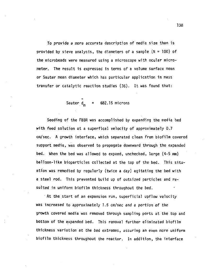
138

To provide a more accurate description of media size than is

provided by sieve analysis, the diameters of a sample (N = 100) of

the microbeads were measured using a microscope with ocular micro-

meter. The result is expressed in terms of a volume surface mean

or Sauter mean diameter which has particular application in mass

transfer or catalytic reaction studies (36). It was found that:

Sauter d = 682.15 micronsm

Seeding of the FBBR was accomplished by expanding the media bed

with feed solution at a superfical velocity of approximately 0.7

cm/sec. A growth interface, which separated clean from biofilm covered

support media, was observed to propagate downward through the expanded

bed. When the bed was allowed to expand, unchecked, large (4-5 mm)

balloon-like bioparticles collected at the top of the bed. This situ-

ation was remedied by regularly (twice a day) agitating the bed with

a steel rod. This prevented build up of outsized particles and re-

sulted in uniform biofilm thickness throughout the bed.

' At the start of an expansion run, superficial upflow velocity

was increased to approximately 1.5 cm/sec and a portion of the

growth covered media was removed through sampling ports at the top and

bottom of the expanded bed. This removal further eliminated biofilm

thickness variation at the bed extremes, assuring an even more uniform

biofilm thickness throughout the reactor. In addition, the interface

139

between seeded and unseeded media near the bottom of the bed, which

served as a datum for all FBBR experimentation, was made more dis-

tinct by this removal. For each experimental run, before superficial

velocity variation was begun, it was necessary to establish the basis

for calculation of bed porosity in terms of the easily observable

parameter, bed height. By the definition of porosity, the following

may be written:

VSe * 1 - -A 5.11HBA

in which Vs = total solids (biofilm + media) volume in H^A.

Thus, if the total solids volume in the expanded bed is known, bed

porosity and bed height are related by the simple expression, Equation

5.11. In this study, V- was determined as follows.

Bioparticles were removed from the laboratory FBBR by carefully

lowering a vial into the expanded bed and allowing it to fill with

growth covered particles. Great care was taken during this opera-

tion to avoid any shearing of biomass from the support particles. An

average bioparticle diameter dp (and thus biofilm thickness 6) was

determined by direct measurement of at least 50 particles using a

microscope with ocular micrometer. After determining bioparticle

diameter, superficial velocity was measured (bucket and stopwatch tech-

HO

nique) and the corresponding expanded bed height Hj, recorded. A

volume of solids was then withdrawn from the reactor through a samp-

ling port and the new expanded bed height fLL noted. The total

and volatile solids concentration of the withdrawn sample was deter-

mined. The support media was separated from the ash which remained

after volatile solids ignition, rinsed, dried and weighed. The

number of bioparticles in AH« - HDU - HDL could then be calculatedb D I DC

using the media density and average diameter as follows:

* particles . mass of media 1n AHB 5 12

the total volume of solids remaining in the growth covered portion of

the expanded bed could then be calculated as:

VS

AHB

# Particles in \ / ir A 3AHB > < 6 dP 5.13

Thus, bed porosity could be related directly to measured bed height by

Equation 5.11.

During an expansion run, superficial velocity was decreased, the

resultant bed height measured and the bed porosity calculated using

Equation 5.11. Superficial velocity was decreased rather than increased

during expansion runs after it was observed that the increase in tur-

bulence associated with the latter procedure caused significant slough-

ing of biofilm which resulted in non-linear log U - log e plots.

141

Examples of FBBR expansion plots are given in Figure 5.11.

The expansion index, n, is the slope of the log U - log e plot.

The procedure outlined above was repeated for several different

biofilm thicknesses i.e., for several dp's. Biofilm thickness was

varied by varying the amount of support media within the FBBR. In

general, the more media used, the thinner were the resultant equi-

librium biofilms.

142

1.0

.8

.6

.5

.4

.3

n = 5.5U n = 5.77 cm/sec.£=1

6 = 88 microns

1.0

.8

,6

.5

.4

n = 4.8

U , = 4.18 cm/sec.e=l

6 = 207 microns

.3 .4 .6 .8 1.0

Figure 5.11 Typical FBBR Bed Expansion Data

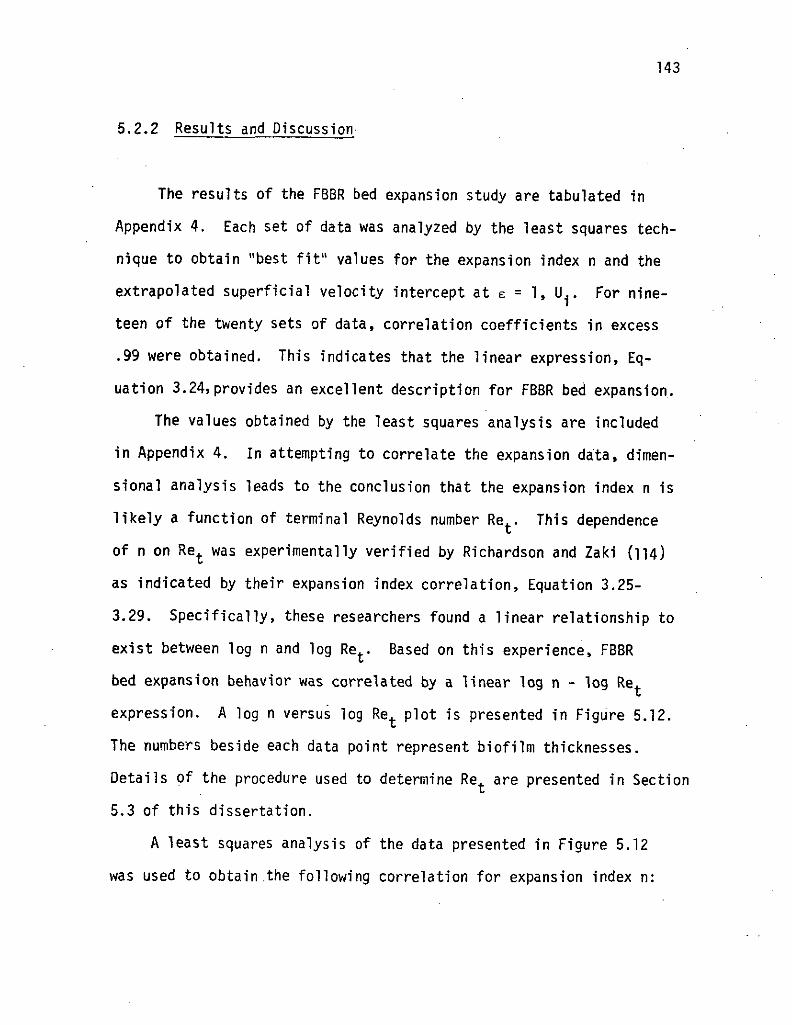
143

5.2.2 Results and Discussion

The results of the FBBR bed expansion study are tabulated in

Appendix 4. Each set of data was analyzed by the least squares tech-

nique to obtain "best fit" values for the expansion index n and the

extrapolated superficial velocity intercept at e = 1, U.. For nine-

teen of the twenty sets of data, correlation coefficients in excess

.99 were obtained. This indicates that the linear expression, Eq-

uation 3.24, provides an excellent description for FBBR bed expansion.

The values obtained by the least squares analysis are included

in Appendix 4. In attempting to correlate the expansion data, dimen-

sional analysis leads to the conclusion that the expansion index n is

likely a function of terminal Reynolds number Re.. This dependence

of n on Ret was experimentally verified by Richardson and Zaki (114)

as indicated by their expansion index correlation, Equation 3.25-

3.29. Specifically, these researchers found a linear relationship to

exist between log n and log Re,. Based on this experience, FBBR

bed expansion behavior was correlated by a linear log n - log Re.

expression. A log n versus log Ret plot is presented in Figure 5.12.

The numbers beside each data point represent biofilm thicknesses.

Details of the procedure used to determine Re, are presented in Section

5.3 of this dissertation.

A least squares analysis of the data presented in Figure 5.12

was used to obtain.the following correlation for expansion index n:

c

c

1.75

1.70

1.65

1.60

1.55

1.50

1.45

1.40

1.35

40

344

n = 10.35 Rel18

L

590

.703

347

.812J005

3.7 - 3.8 3.9 4.0 4.1 4.2 4.3 4.4 4.5 4.6 4.7

in Re_

Figure 5.12. Expansion index versus Reynolds number; a log-log plot.

145

n = 10.35 Re-.18 5.14

It is noted that the correlation coefficient for this equation is only

-.43. Because of this low correlation coefficient, a statitistical

test for independence was performed on these data. The null hypo-

thesis, Ho : p = 0, was rejected at the 10 percent level of signi-

ficance indicating statistically significant correlation of .n with Re..

Although this low correlation coefficient indicates significant dif-

ferences between observed and predicted (by the correlation) values of

expansion index, it can be shown that the bed porosity-superficial

velocity relationship is rather insensitive to these differences.

Consider the 6 = 1005 micron data point of Figure 5.12 which lies

far from the best fit line. The expansion observed for this film

thickness was 4.01; that calculated by the correlation equation is

4.64. The error in the predicted value is approximately 16 percent.

Now, assuming a typical superficial velocity of 0.8 cm/sec and using

the observed intercept velocity of 2.69 cm/sec, bed porosities are

calculated below using both the observed and the correlation expansion

indices:

observed, n = 4.01: e -.8

2.69

1/4.01= .74

correlation, n = 4.64 .82.69

1/4.64.77

146

a difference of only 4 percent.

For comparison sake, the correlation developed by Richardson and

coworkers (113, 114) for rigid spheresin similar Re. range is pre-

sented here. By assuming the aspect ratio dp/D to be negligible, the

correlation developed by these researchers may be written as:

n = 4,4 Re^/1 1 < Ret < 500 5.15

It is noted that, as expected, expansion indices observed in the

FBBR are uniformly higher than predicted by the Richardson-Zaki cor-

relation, Equation 5.1. In addition, the correlation developed here

indicates a stronger dependence of expansion index n on Ret than ob-

served with rigid spheres. And finally, the expansion behavior of a

FBBR appears to be less "quantifiable" than possible with rigid parti-

cles. This is evidenced by the significant scatter of data shown in

Figure 5.12.

As mentioned in Section 4.2, it has been reported in the liter-

ature (49) that biofilm volatile solids density pD is a function ofD

biofilm thickness 6. Although clear evidence of this dependence was

not observed in the ROR portion of this study (which was limited to

relatively thin biofilms), a pronounced dependence of density on film

thickness was observed in the FBBR. This is indicated in Figure

5.13. The solid lines shown in Figure 5.13 were drawn by eye and are

described, mathematically by Equations 4.17 a, b and c.

to

en

c:<uQ

80

70

60

50

-' o

o•r—CO

30

20

10

J ! J I

0 .02 .04 .06 .08 .1 .12 .14 .16

Biofilm Thickness (cm)

Figure 5.13. Biofilm V ,S . density versus biofilm thickness.

148

5,3 Fluidized Bed Biofilm Reactor - Bioparticle Terminal Velocity

The objective of this segment of the experimentation was to

develop a drag coefficient-Reynolds number correlation which could be

used, with Equation 4.20, to predict the terminal velocity of a bio-

particle.

The bioparticle terminal velocity determination served a dual

purpose in that it provided a basis for prediction of the expansion

curve superficial velocity intercepts at e = 1, U. and it provided the

terminal Reynolds numbers needed in developing the expansion index -

terminal Reynolds number correlation presented in Section 5.2.

5.3.1 Materials and Methods

Equation 4.20 can be rearranged so that drag coefficient can be

expressed in terms of observable quantities as:

4 (PC - P. ) 9 dpC = 5 L v_ 4^20U i no

For a given experimental run, the average bioparticle diameter dp, was

determined as described in Section 5.2. Also determined in Section 5.2

were the total solids, volatile solids, mass of support media and num-

ber of support particles in the sampled segment of the FBBR. Thus,

149

bioparticle density, ps, could be calculated as outlined in the fluidi-

zation algorithm of Section 4.2.

As described in Section 5.2, during each experimental run a bio-

particle sample was carefully removed from the expanded bed and a

portion of the sample used to determine an average bioparticle

diameter. The remainder of the sample was allowed to settle through

a 14 cm ID x 195 cm water filled plexiglass column. By timing parti-

cle descent through a 120 cm segment of the column, terminal velocity

was determined. At least fifty individual settlements were conducted

for each biofilm thickness. The individual measurements were aver-

aged to obtain the terminal velocity representative of the given bio-

film thickness.

The properties of the fluid phase, p, and u, were determined

by relating tabulated values (106) to the water temperature measured

in the settling column.

The information needed to calculate drag coefficient using Eq-

uation 4.20 was, therefore, available.

The corresponding terminal Reynolds number was, in turn, calcul-

ated using Equation 4.23.

By repeating the procedure outlined above for FBBR experimental

runs with different equilibrium biofilm thicknesses, a data base for

the drag coefficient-Reynolds number correlation was obtained.

150

5.3.2 Results and Discussion

For each of the twenty FBBR experimental runs, terminal Rey-

nolds number and the corresponding drag coefficient were determined,

as described in Section 5.3.1. A log-log plot of these data is

given in Figure 5.14. A least squares analysis was used to obtain

the best fit line shown in this figure. The resultant drag coef-

ficient-Reynolds number correlation, which is specific for FBBR bio-

particles, was presented in Chapter 4 as:

= 36.66 Re2/3 4.21

The correlation coefficient for the expression is -.74.

Combining this correlation equation with Newton's law, Equation

4.20, an explicit expression for bioparticle terminal velocity is ob-

tained. This expression was also presented in Chapter 4 as Equation

4.22.

3/4

U.-PL)

27.5 PL1/3 2/3 4.22

oo

1.8

1.6

1.4

1.2

1.0

.8

.6

.4

.2

3.5

Cp=36.66 Re-2/3

3440

1680

4.0 4.5 5.0

In Re

Figure 5,14 Log-log Plot of Drag Coefficient vs. Reynolds Number

151

152

5.4 Fluidized Bed Biofilm Reactor - Biomass Holdup and Nitrate Profiles

In this section, biomass holdup and nitrate profiles measured in

the laboratory FBBR are compared with values predicted by the FBBR are

compared with values predicted by the FBBR mathematical model. Input

parameters to the FBBR model include the nitrate effective diffusivity

and intrinsic Michaelis-Menten coefficients determined in the RDR ex-

perimentation. Input correlations to the FBBR model, developed as

part of this research, relate biofilm volatile solids density, to_

biofilm thickness, drag coefficient to Reynolds number and expansion

index to terminal Reynolds number.

5.4.1 Materials and Methods

The laboratory FBBR and its operation were described in Section

5.2. Nitrate profiles through the reactor were obtained by the fol-

lowing procedure. During each bed expansion run (cf. Section 5.2)

flow variation was interrupted to allow the nitrate concentration

distribution throughout the bed to be measured. To avoid any trans-

ients which result from altered upflow velocity and concentration, at

least one half hour (roughly ten detention times) was allowed to

elapse between a flow variation and a nitrate profile measurement.

After this period, several nitrate profiles were taken to assure that

steady-state had been realized. Steady-state was assumed when.no

153

significant variation in nitrate concentration was noted between suc-

cessive profiles.

Nitrate-nitrogen profiles were obtained by withdrawing liquid

samples from five screened sampling ports along the length of the

reactor. Additional samples were obtained at the reactor inlet and

overflow. Samples were withdrawn in order of largest to smallest

space time, T = ZA/Q. To minimize hydraulic upset of the expanded bed,

the rate of liquid sample withdrawal was kept below two percent of the

upflow rate.

Samples were analysed for nitrate-nitrogen using an Orion specific

ion meter Model 407A with an Orion specific ion electrode Model 93-07.

In addition to nitrate measurements, dissolved oxygen, pH and

temperature were also monitored during FBBR experimentation.

Dissolved oxygen levels in the FBBR influent were under 0.2 mg/1

for all runs. Effluent dissolved oxygen concentrations, measured by

lowering the DO probe directly into the experimental reactor were con-

sistantly zero.

Influent pH was found to be 6.9 ± .1. Hydroxide ion produced dur-

ing biological reduction of nitrate caused an increase in pH across

the FBBR'of up to one unit.

The liquid temperature during all experimental runs was 21 C ± 2 C.

To predict Diomass no'iaup ana suostrate conversion in the labora-

tory reactor using the FBBR model, a total of thirteen parameters and

154

six correlations must be specified. Numerical values for the para-

meters used in generating the predicted values presented in this

section are given in Table 5.2.

5.4.2 Results and Discussion

For each of the twenty biofilm thicknesses examined in this re-

search, a nitrate profile through the laboratory FBBR was measured.

Typical plots showing observed and predicted values for biofilm thick-

ness, total volatile solids concentration and nitrate profiles are

presented in Figures 5.15, 5.16 and 5.17. Data for the other experi-

mental runs is presented in Appendix 4.

In general, there was good agreement between conditions observed

in the laboratory FBBR and those predicted by the mathematical model.

It was observed, however, that as biofilm thickness increased beyond

300 microns, the ability of the model to accurately predict nitrate

reduction decreased significantly. This phenomenon is probably linked

to the decreasing biofilm volatile solids density observed in this film

thickness region. A possible explanation for this is that the biofilm

parameters k, KS and D~B may not be independent of biofilm density as

assumed in development of the model. It seems especially unlikely

that the effective diffusivity DSB would be unaffected by variation in

biofilm density. Unfortunately, detailed study of this phenomenon was

not possible in the rotating disk reactor due to the limitation to rela-

tively thin biofilms imposed by the turbulent conditions within the RDR.

155

Table 5.2 FBBR Model - Numerical Values for Input Parameters.

DSL = 1.67 E-5 cm /sec

PL = .998 g/cm

y = .009548 g/cm-sec2

DSB = .815 E-5 cm /sec

k = 3.32 E-5 /sec

KS = 6.06 E-8 g/cm3

S.JZ=0 = specify for each run

Q = specify for each run

A = 11.4 cm2

HB = specify for each run

Pm = 2.42 g/cm3

dm = 682 E-4 cm

V = specify for each run

28 -

24

20 -

16 -

12 -

8 -

4 -

X(mg VS/1)

10016

10146

00 Observed

— Predicted

20 40 60 80 100 120 140 160 180 200 220en

Figure 5.15 Observed and predicted nitrate profiles for the laboratory FBBR.

28

24

20 '

,« 16o

12 •

4 '

oo Observed 207 (1784Predicted 215 13063

20 40 60 80 100 120 140 160 180 200 220

Figure 5.16 Observed and predicted nitrate profiles for the laboratory FBBR

28

24

SF 20

i no

00 Observed 1005

— Predicted 1035

X(mg VS/1)

7649

7893

20 40 60 80 100 120 140 160 180 200 220T (sec)

Figure 5.17 Observed and predicted nitrate profiles for the laboratory FBBR. tnCO

C H A P T E R V I

E N G I N E E R I N G APPLICATIONS

As developed in the fourth chapter of this dissertation,

f luidized bed b i o f i l m reactor performance is affected by five para-

meters which are under the direct control of the design engineer.

These parameters are listed below:

1) Expanded bed height, HB;

2) Reactor area perpendicular to flow, A;

3) Support media density, p ;

4) Support media diameter, d ;

5) Support media volume, V .r m

A parameter which is indirectly controllable by the design

engineer is the equilibrium biofilm thickness, 6. For a given media

(dm and p ), equilibrium biofilm thickness is dependent on super-m m ^ r

ficial upflow velocity, expanded bed height and support media volume.

Biofilm thickness is, in turn, the single most important parameter

affecting biomass effectiveness and hence the overall performance of

a FBBR.

A concept which aids in understanding the performance charac-

teristics of a FBBR is that of effective biomass (actually effective

159

160

volatile solids) concentration within the reactor. The effective V.S.

concentration is less than total foiomass concentration because of

diffusional limitations; it is defined here as the product of effec-

tiveness factor and the reactor total volatile solids concentration.

Effective V.S. concentration, X-, may therefore be written as: .

_ v volume of biomassA " no X = no PB ' 6.1

volume of expanded bed .

Effective V.S. concentration is, in turn, related to the overall re-

action term R of Equation 4.3 as follows:

k shRv = XA —-A

Thus, the rate of reaction at any point in a FBBR is directly propor-

tional to the effective V.S. concentration at that ooint. Maximiza-

tion of effective V.S. concentration will therefore maximize the over-

all rate of substrate conversion in the FBBR. Optimization of FBBR

performance is, however, not a straightforward process because ef-

fectiveness factor, and hence effective V.S. concentration, will vary

with bulk substrate concentration through the reactor.

As background to an understanding of this phenomenon, the rela-

tionship between total volatile solids concentration and equilibrium

biofilm thickness must be determined. The fluidization alaorithm of

161

Section 4.2, with modifications, serves as the basis for this deter-

mination. The required modifications are as follows:

Step 1. Specify a biofilm thickness, 6.

Step 10. Calculate the total volatile solids concentration

X as:

X = PR (1 - e) [ 1 - (d / d ) 3] 6.3D |_ m p J

Step 11 and 12. delete

The modified algorithm was used to develop the total volatile

solids versus biofilm thickness curves of Figure 6.1. Additional

information needed to generate these curves was provided earlier in

Table 5.1, Note that these curves are specific to the given upflow

velocities and media characteristics. The rather abrupt slope changes

around biofilm thicknesses of 0.03 and 0.063 cm. are due to the abrupt

slope changes in the p - 6 correlation at these points (cf. EquationD

4.17).

If the objective were simply to maximize total volatile solids

concentration for the given media characteristics, the FBBR should be

operated so as to control biofilm thickness at approximately 0.03 cm.

Because of diffusional limitations, however, this simplistic approach

may not optimize overall performance of the FBBR. To examine this

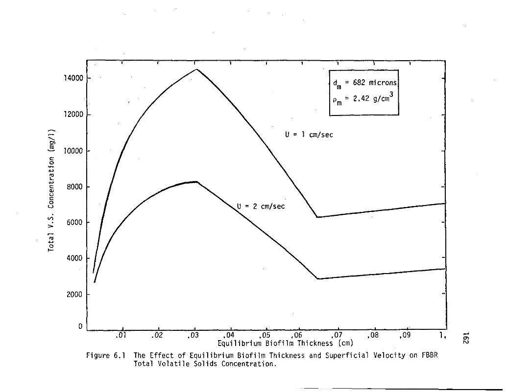
co

to

CQJOCoo

14000

12000

10000

8000

6000

4000

2000

d = 682 micronsm=2.42 g/cin33

.01 .02 .03 ,08 ,09,04 ,05 ,06 ,07Equilibrium Biofilm Thickness (cm)

Figure 6.1 The Effect of Equilibrium Biofilm Thickness and Superficial Velocity on FBBRTotal Volatile Solids Concentration.

'ro

163

possibility, it is necessary to determine the effect of biofilm thick-

ness on the biofilm effectiveness factor. The mathematical background

for this determination is developed in Section 4.3.

For a single bulk substrate concentration (in this case

S, = 20 mg/1 NO- - N), numerical .solutions of Equations 4.34 and

4.39 yield the effectiveness factor versus biofilm thickness plot

shown in Figure 6.2.

The rather strange (as compared to catalysis) shape of this curve

over the interval 0.03 < 6 < 0.063 cm is due to the variable vola-

tile solids density PB in this region. In Section 4.3, it is shown

that biofilm effectiveness factor is dependent on a Thiele-type

modulus given as:

Lk PB

SbDSB

As the modulus increases in magnitude, the effectiveness factor

decreases. In the biofilm thickness region mentioned above, the

impact of increases in film thickness on the modulus and hence the

effectiveness factor are countered by decreases in biofilm vola-

tile solids density. This competitive phenomenon causes the effec-

tiveness factor curve to level in this region and, in fact, show a

slight upward trend in the neighborhood of 6 = 0.063 cm.

Superimposed on the effectiveness factor curve is the total

volatile solids concentration versus biofilm thickness plot of Figure

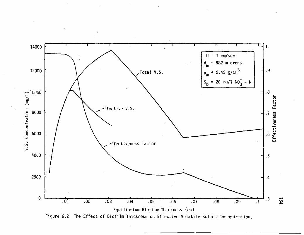
14000

12000

10000

J 8000-U

C<Duco(-J

6000

4000

2000

1 cm/sec

682 microns

= 2 . 4 2 g/cm3

= 20 mg/1 - N

effectiveness factor

1.

.9

.8o•MU

(U

Ufi <UD u_

.02 .08 .09.03 .04 .05 .06 .07

Equilibrium Biofilm Thickness (cm)Figure 6,2 The Effect of Biofilm Thickness on Effective Volatile Solids Concentration,

.1

.5

.4

•3

165

6.1 for a superficial upflow velocity of 1.0 cm/sec. Information

given by these two curves is used to calculate the effective vola-

tile solids concentration curve, also shown in Figure 6.2.

Observe that although total volatile solids concentration is

maximized by controlling biofilm thickness at approximately 0.03

cm, the effective volatile solids concentration for the listed condi-

tions is a maximum at a biofilm thickness of approximately 0.012 cm.

In fact, for the given case, the effective volatile solids concentra-

tion at a biofilm thickness of 0.03 cm is approximately 25 percent

less than its maximum value.

For a constant bulk substrate concentration, selection of an

optimum biofilm thickness at which to operate the reactor is a re-

latively straightforward matter. However in a real FBBR, bulk

substrate concentration, and therefore, effectiveness factor and

effective biotnass concentration, vary with space time through the

reactor. To illustrate this phenomenon, effectiveness factor versus

biofilm thickness curves for several bulk substrate concentrations

are presented in Figure 6.3. Note that as S. decreases, the biofilm .

thickness which maximizes X. also decreases.

To more clearly show the effect of variations in bulk substrate

concentration on effective V.S. concentration, the data of Figure 6.3

are reworked to yield the plots shown in Figure 6.4. For each of the

curves of Figure 6.4, effective V.S. concentration approaches total

V.S. concentration (from Figure 6.1) as effectiveness factor approaches

unity.

166

14000

12000 -

10000

- 8000en

'5 6000t--MCOJU

<§ 4000

S 2000

0

Sb = 20 mg/1 NO- - N

Sb = 10.mg/1 N03 -N

Sfa = 5 mg/1 N03 -

.03 .03 .04 .05 .06Equilibrium Biofilm Thickness (cm)

Figure 6.3 The Effect of Equilibrium Biofilm Thickness on FBBRTotal V.S. and Effectiveness Factor.

CTl

Co

s-4Jc(Uuc:o

CO

OQJ

<*-

10000

8000

6000

<u 4000 -

2000

0

u =dm =pm =

1 cm/sec682 microns

2.42 g/cm3

123

4

6 (microns)

150

200

100

50

X (mg/1 V.S.)

1187713049

9926

6474

10 15 40_ 20 25 30 35Og - N Concentration (mg/1)

Figure 6,4 The Effect of Bulk-liquid Substrate Concentration of FBBR EffectiveVolitile Solids Concentration,

en

168

The relative importance of effectiveness factor and total V.S.

concentration in determining the effective V.S. concentration can be

brought into focus by examining specific regions of the X. - S. plots

of Figure 6.4. For the listed flow and media characteristics, con-

sider the objective to be selection of an optimum biofilm thickness

for the reduction of nitrate-nitrogen concentration from 30 to 25

mg/1. It is apparent that effective V.S. concentration over this

region is maximized by operation of the FBBR to maintain biofilm thick-

ness in the 150 micron range. Both the 50 and 100 micron biofilms

have effectiveness factors which approach unity in the given S. range;

however, both effective V.S. concentrations are limited by the corres-

ponding, relatively low, total V.S. concentrations. In contrast,

the 200 micron biofilm has the highest total V.S. concentration of

the biofilms examined, but the effective V.S. concentration is limited

by biofilm effectiveness factor. The 150 micron biofilm maximizes

effective V.S. concentration over the given Su range because it has an

optimum combination of total V.S. concentration and effectiveness

factor.

As bulk substrate concentration decreases, the importance of

diffusional limitations increases. This is illustrated by focusing

on the 0 to 5 mg/1 NO, - N region of Figure 6.4. It can be seen that

although the 50 micron biofilm has the lowest total V.S. concentra-

tion of the thicknesses examined, it has the highest effective V.S.

concentration over this region. This is due to the fact that the

169

thicker biofilms are severely limited by transport, resistances at

low bulk substrate concentrations.

The impact of biofilm thickness on nitrate-nitrogen concentra-

tion profiles generated using the FBBR mathematical model is illus-

trated by Figure 6.5. This figure shows clearly that to optimize

substrate conversion the FBBR should not be operated to maximize

total V.S. concentration (200 micron biofilm) or to maximize ef-

fectiveness factor (50 micron biofilm) but rather to maximize the

product of these parameters throuqhout the reactor.

Thus far in this chapter, an attempt has been made to demon-

strate the utility of being able to exercise control of biofilm

thickness within a FBBR. The mathematical model for biofilm bed

fluidization developed as part of this research is advanced as a

rational basis for selection of design parameters to yield a desired

biofilm thickness.

Consider the following examples.

EXAMPLE 1. For a given reactor and inflow, determine the volume

of a specified support media which will yield an equili-

brium biofilm thickness of approximately 100 microns.

GIVEN: HB = 200 cm p = 2.42 q/cm3

A = 100 cm2 dm = 682 microns

Q = 100 cm3/sec 6fiq = 100 microns

Co

ucoCJ

0)D-.oS--I-J

30

25

20

15

£ 10

'U=l cm/sec P =2.42g/cr,r

So=30 mg/1 dm=682 microns'm

6511

9947

11,885

13,142

10 20 30 40 50 60Space Time (sec)

70 80 90 100

Finure 6.5 The Effect of Biofilm Thickness on Nitrate Conversion in aFBBR as predicted by the FBBR Mathematical Model.

171

FIND: V .m

SOLUTION: Equation 4.16

Equations 4.17, 4.18

and 4.19

Equation 4.22

Equation 4.23

Equation 4.24

Equation 4.25

dp = 882 microns

PS

Ut

Re

n

e =

1.70 g/cm

5.50 cm/sec

= 50.7

5.1

.716

Vm = HB A dP>

Vm * (200 cm) (100 cm2) (1 - .716) (682 y/882y)3

Vm = 2626 cm3

The solution scheme used in the preceeding example was used to

develop Figure 6.6. The following is an alternate solution proce-

dure for Example 1, which utilizes Figure 6.6.

SOLUTION: From the 100 micron curve of Figure 6.6;

at U = 1. cm/sec:

172

160

140

120

00

CQ80

60

40

20

Pm = 2.42 g/cm°

d = 682 microns

1.5 2.

U (cm/sec)2.5 3. 3.5

Figure 6.6 The Effect of Biofilm Thickness on FBBR Bed Expansion

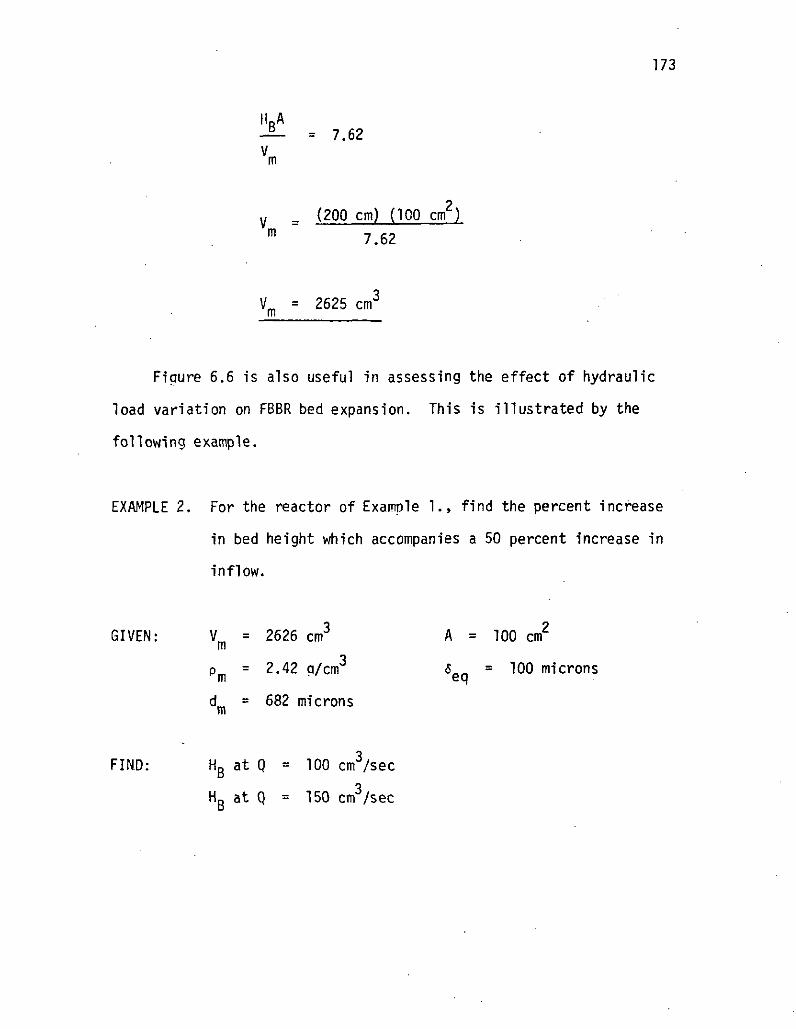
173

ILA-£- = 7.62Vm

V = (200 cm) (100 cm2)m " 7.62

Vm = 2625 cm3

Fiqure 6.6 is also useful in assessing the effect of hydraulic

load variation on FBBR bed expansion. This is Illustrated by the

following example.

EXAMPLE 2. For the reactor of Example 1., find the percent increase

in bed height which accompanies a 50 percent increase in

inflow.

GIVEN: Vm = 2626 cm3 A = 100 cm2

p = 2.42 a/cm3 6 = 100 microns

d = 682 micronsm

FIND: HB at Q = 100 cm3/sec

HB at Q = 150 cm3/sec

174

3SOLUTION: From Example 1., at Q = TOO cm , HB = 200 cm.

From the 100 micron curve of Figure 6.5; at U = 1.5 cm/sec

HR A-£— = 9.62Vm

u : (9.62) (2626 cm3)H _ .

b 100 cnT

HD = 252.6 cmD

The percent increase in HB which accompanies this 50

percent increase in inflow is:

AHD = 26.3 percentD

As discussed earlier, thin biofilm tends to maximize effective-

ness factor. Figure 6.6 shows that thin biofilm in a FBBR is also

advantageous from the standpoint of bed stability against hydraulic

load, variation. This is shown in the example below.

EXAMPLE 3. For the reactor and media of Examples 1 and 2, find the

percent increase in bed expansion which accompanies a 50

percent increase in upflow velocity (1. to 1.5 cm/sec)

for a biofilm thickness of 300 microns.

GIVEN: Vm = 2626 cm0

pm = 2.42 g/cm3

d = 682 microns

A = 100 cm"

fi = 300 micronseq

FIND: HD at 0 * TOO cnT/sec0

HD at Q = 150 cm3/secD

SOLUTION: From the 300 micron curve of Figure 6.6; at U = 1.0 cm/sec

25.6

m

H _ (25.6) (2626 cm)* - 5b 100 cm^

HB = 672 cm

At U = 1.5 cm/sec

= 33.7

= (33.7) (2626 cnT)

100 cm2

176

HD = 885 cmD

The percent increase in Hg which accompanies this 50

percent increase in inflow is:

AHB = 31.7 percent

Even more significant than the percent increase in bed height is

the actual magnitude of the bed height increase. For the 100 micron

biofilm, the 50 percent increase in inflow causes a 52.6 cm increase

in bed height. For the 300 micron biofilm, the same increase in in-

flow results in a bed height increase of 213 cm.

The previous examples have focused on the bed expansion-biomass

holdup portion of the FBBR mathematical model. The following ex-

ample more fully utilizes the comprehensive biomass holdup and sub-

strate conversion capabilities of the model.

EXAMPLE 4. Design a FBBR which will reduce influent nitrate-nitrogen

concentration from 30 to 3 mg/1. The reactor is to uti-

lize the media of the previous examples and operate at

a biofilm thickness of approximately TOO microns and a

superficial velocity of 1 cm/sec. Specifically, deter-

mine the combination of V and HD which will result inm B

an effluent nitrate-nitrogen concentration of 3 mg/1

under the stated conditions.

177

GIVEN: Q = 100 cm/sec

A = 100 cm2

d = 682 microns

pm = 2.42 g/cm

6 = 100 microns

Sb|z=:0 = 30 mg/1

Sb'z=H = 3

8

FIND: and

SOLUTION: Computer solution of this problem involves a slight modi-

fication of the fluidization portion of the FBBR model.

Rather than specifying V and HB and calculating biofilm

thickness, V and 6 are specified and the resultant H0m r D

calculated. For the given biofilm thickness, V is varied

until S- = 3 mg/1 at Z = Hg. The computer solution to

this example is presented in Table 6.1.

The effect of support media characteristics on FBBR performance,

as predicted by the FBBR mathematical model, will be examined briefly.

Figures 6.7 and 6.8 present effective V.S. concentration as a function

of superficial velocity and biofilm thickness for a range of support

media characteristics. A bulk substrate concentration of 10 mg/1

nitrate-nitrogen was used in developing these figures.

It is apparent that decrements in superficial velocity or in-

crements in either support media density or size, increases effective

V.S. concentration. In general, the computer simulations of this

study indicate that substrate conversion is maximized when bed poro-

190220230270200RNH

0=100*XA--100*HB=117»3Yh-1540,30-30. E--6

model input

DEL-DP-EP-

,01000,08820,71603

.00992450

6,62736

TAU N03-N ETA

0,5,865000011,730000017.595000023*460000029,325000035.190000041,055000046,920000052,785000058,650000064.515000070,380000076.245000082,110000087,975000093,8400000

. 99.7050000105.5700000111.4350000117,3000000

END.

0.5.865000011,730000017.595000023,4600000 .29.325000035,190000041.055000046,920000052.785000058,650000064,515000070*380000076.245000082.110000087.975000093.840000099,7050000105,5700000111,4350000117.3000000

,0000300,0000281,0000262,0000243,0000224,0000205.0000186.00001.63,0000151.0000134.0000119,0000104,0000091,0000079,0000068,0000058,0000049.0000042,0000036,0000032,0000030

,9989077,9986959.9984138,9980236.9974619,9966028,9951644,9923694,9849935.9558097.9019762,8447467,7869991,7291665,6717472,6153268,5609046,5100013,4653947.4319402.4180686

SRU 66.349 UNTS.

• RUN COMPLETE,

Table 6.1 FBBR model computer output {see Appendix 11 for a descrip-tion of program nomenclature).

178

CJocoo

<D

OOJ

12000

10000

8000

6000

4000

2000

U=l cm/secdm = 682 micronsmS. = 10mg/l NOl - N

pm=4.5 g/1cmv

U=2 cm/secd - 682 micronsSh = 10mg/l NO! - N

.01 .02 .03 .04Equilibrium Biofilm Thickness (cm)

.01 .02 .03 .04Equilibrium Biofilm Thickness (cm)

Figure 6.7 Effect of Support Media Density on Effective Volatile Solids Concentration.

Co

rej-•pE=QJOCOCJ

OJ

GJ4-

UJ

12000

10000

8000

6000

4000

2000

0

U=l cm/sec qp = 2.42 g/cnrmSfc=10 mg/1 NO^ - N

POO microns

682 microns

300 microns

u=z cm/sec

pm=2.42 g/cm3

Sb=10 mg/1 NO^ - N

1000 microns

682 microns

300y(washout)

.01 .02 .03 .04Equilibrium Biofilm Thickness (cm)

Figure 6.8 Effect of Support Media Diameter on Effective Volitile Solids Concentration.

.01 .02 .03Equilibrium thickness (cm)

.04

00o

181

sity is minimized.

The effect of support media characteristics on FBBR bed expan-

sion is presented, graphically, in Figures 6.9 and 6.10. These figures

show that FBBR bed height stability to variations in superficial velo-

city, increases with increased media size or density. This is ex-

tremely important with regard to flow equilization requirements for

a system utilizing a fluidized bed reactor.

In summary, it appears that the use of larger or denser support

media in a fluidized bed biofilm reactor offers advantages, as dis-

cussed above. Any such advantage, however, must be weighed against

the higher energy requirements for fluidization of these media. In

addition, problems such as bed clogging, particle-particle bridging

and gas entrapment may accompany low porosity operation of a FBBR using

larger or denser support media.

182

CD1C

160

140

120

100

80

60

40

20

d = 682 micronsm

6 = 200 microns

Pm = 1.4 g/cnf

Pm = 2.42 g/crn'

0 .5 1. 1.5 2. 2.5 3

U (cm/sec)

Figure 6.9 Effect of Support Media Density on FBBR

Bed Expansion

183

180

160

140

120

TOO

80

CO

60

40

20

m = 2.42 p/cmj

5 = 200 microns

d = 300 micronsm

d, = 682 micronsm

d = 1000 micronsm

0 .5 1.5 2U (cm/sec)

2.5

Figure 6,10 Effect of Support Media Diameter on FBBRBed Expansion.

C H A P T E R V I I

SUMMARY, CONCLUSIONS AND RECOMMENDATIONS

Summary

The fluidized bed biofilm reactor is a novel biological waste-

water treatment process. The use of small, fluidized particles in

the reactor affords growth support surface an order of magnitude

greater than conventional biofilms systems, while avoiding clogging

oroblems which would be encountered under fixed bed operation. This

allows retention of high biomass concentration within the reactor.

This high biomass concentration, in turn, translate to substrate con-

version efficiencies an order of magnitude greater than possible in

conventional biological reactors.

The primary objective of this research has been the development

of a mathematical model of the fluidized bed biofilm reactor. This

model identifies five contro31able parameters (A, HB, V , p , d )

which effect reactor performance and thus, provides a rational basis

for reactor design. The mathematical model has two major subdiv-

isions. The first predicts biomass holdup within the reactor using

drag coefficient and bed expansion correlations developed as part

of this research. The second predicts mass transport-affected sub-

strate conversion by biofilm covering individual support particles.

184

185

Intrinsic kinetic coefficients and effective diffusivity for bio-

film denitrification, used in this segment of the model, were deter-

mined in an independent study.using a rotating disk biofilm reactor.

Conclusions

1. The FBBR model adequately predicts nitrate-limited denitrifica-

tion within a fluidized bed biofilm reactor, especially for bio-

film thickness under 300 microns.

2. The most significant parameter affecting substrate conversion ef-

ficiency in a fluidized bed biofilm reactor is biofilm thickness.

3. Biofilm thickness, and thus FBBR performance can be controlled

through specification of the following design parameters:

Expanded bed height, HD;0

Reactor horizontal area, A

Support media density, p ;

Support media diameter, d ;rr » m>

Support media total volume, V .

4. The FBBR model provides a rational basis for selection of design

parameters.

5. The biofilm denitrification parameters D«-B, k and K- obtained in

the rotating disk reactor study are applicable to denitrification

in a fluidized bed reactor for similar biofilm thicknesses.

186

6. From the rotating disk reactor study, the following 95 percent

confidence intervals were determined for the denitrifying bio-

film parameters D-R, k and K.:

0.198 x 10"5 < DSB (nitrate) < 1.432 x 10"5 cm2/sec

2.873 < k < 2.878 day"1

0 < KS < 0.3077 NO^ - N

for pH = 6.92 + .1, temperature = 22°C + 1°C and biofilm

thickness < 300 microns.

7. Biofilm volatile solids density was found to decrease with bio-

film thickness between roughly 300 and 630 microns.

8. For the support media and substrate concentration range used in

this study, the FBBR model predicts optimum denitrification when

biofilm thickness is controlled at approximately 100 microns.

Larger or denser suoport media or higher substrate concentration

will shift this optimum toward thicker biofilm.

9. The FBBR model predicts maximum denitrification oer unit reactor

volume when design parameters are specified which minimize bed

porosity while controlling biofilm thickness near its optimum.

Bed porosity is minimized by large or dense support media and

large reactor horizontal area.

187

Recommendations

The following are recommendations for future research:

1. That the FBBR model be verified us ing a pilot-scale denitrifica-

tion f lu id ized bed reactor.

2. That the data base for the FBBR drag coefficient and bed ex-

pansion index correlations be extended by examining a wide ranae

of support media of various densities and sizes.

3. That a b i o f i l m model be developed which describes reaction under

mul t ip le or sequential substrate control.

4. That the effect of b i o f i l m volat i le solids density on effective

di f fus iv i ty and the Michaelis-Menten constants be examined.

5. That a more rational parameter that volati le solids density be

used in analysing for effective d i f fus iv i ty and rate constants;

adenosine tr iphosphate concentration (ATP) is suggested.

6. That the effect of environmental conditions such as pH and tem-

perature on the b i o f i l m deni t r i f icat ion parameters D^n, k and KS

be examined.

7. That the effect of these environmental conditions be incorporated

in the FBBR model.

8. That the FBBR model be extended to biochemical systems other than

deni t r i f icat ion.

Bibliography

1. Adler, I.L., and Happel, J., "Fluidization of uniform spheres inliquid media." Chem. Eng. Prog., Symp. Ser. 58, 98 (1962).

2. Atkinson, B. and Daoud, I.S., "The analogy between microbial re-actions and heterogeneous catalysis." Trans., Inst. Chem. Engrs.46, T19 (1968).

3. Atkinson, B. and Daoud, I.S., "Diffusion effects within microbialfilms." Trans., Inst, Chem. Engrs. 48, T245 (1970).

4. Atkinson, B., Daoud, I.S., and Williams, D.A., "A theory for thebiological film reactor," Trans., Inst. Chem. Engrs. 46, T245 (1968)

5. Atkinson, B., and Davies, I.J., "Overall rate of substrate uptakeby microbial films. I. Biological rate equation." Trans., Inst.Chem. Engrs. 52, 248 (1974).

6. Atkinson, B., and How, S.Y., "The overall rate of substrate up-take by microbial films; Part II. Effect of concentration andthickners." Trans., Inst. Chem. Engrs. 52, 384 (1974).

7. Atkinson, B., and Knights, A.J., "Microbial film fermenters: theirpresent and future applications." Biotech. Bioeng. 17, 1245 (1975).

8. Baillod, C.R,, "Mass Transfer of Glucose through Bacterial Floe,"Ph.D. Dissertation, University of Wisconsin (1968).

9. Baillod, C.R., and Boyle, W.C., "Mass transfer limitations insubstrate removal." Jour. San. Eng. Div., A.S.C.E. 96, 525 (1970).

10. Barnea, E., and Mizrahi, J., "A generalized approach to the fluiddynamics of particulate systems. Part 1. General correlation forfluidization and sedimentation in solid multiparticle systems."Chem. Eng. Jour. 5, 171 (1973).

1.1. Barth, E.F., Brenner, R.C., and Lewis, R.F., "Chemical-biologicalcontrol of nitrogen and phosphorous in wastewater effluent." Jour.Water Poll. Contr. Fed. 40, 2040 (1968).

12. Beek, W.J., "Mass transfer in fluidized beds." in Fluidization,eds, J.F. Davidson and D. Harrison, Academic Press, London andNew York, (1971).

188

189

13. Beer, C., "Evaluation of Anaerobic Denitrification Processes."Jour. San. Eng. Div., A.S.C.E. 96, 1452 (1970).

14. Bird, R.B., Stewart, W.E., and Lightfoot, E.N., Transport Phen-omena, John Wiley and Sons, New York (1960).

15. Bischoff, K.B., "A Note on Boundary Conditions for Flow Reactors."Chem. Eng. Sci. 16, 131 (1961).

16. Brinkman, H.C., "Theory of liquids", Physica 7, 747 (1940).

17. Bruinzeel, C., Reman, G.H., and van der Laan, E.T., "The Inter-actions Between Fluids and Particles." Third Congress of theEuropean Fed, of Chem. Enqrs. p 120 C\962j~.

18. Bungay, H.R., Whalen, W.J., and Sanders, W.M., "Microprobe Tech-niques for Determining Diffusivities and Respiration Rates inMicrobial Slime Systems," Biotech, and Bioeng. 11, 765 (1969).

19. Button, O.K., and Carver, J.C., "Continuous Culture of Torulop-sis utilis: A Kinetic Study of Oxygen Limited Growth." Journalof General Microbiology 45, 195 (1966).

20. Cairns, E.J., and Prausnitz, J.M., "Longitudinal mixing in packedbeds" Chem. Eng. Sci., 12, p 20 (1960).

21. Carberry, J.J., Chemical and Catalytic Reaction Engineering, Mc-Graw Hill, New York (1976).

22. Chambre, P.L., and Acrivos, A., "On Chemical Surface Reactionsin Laminar Boundary-Layer Flow." Jour. Applied Physics 27, 1322(1956).

23. Chang, J.P., and Morris, J.E., "Studies on the utilization ofnitrate by Micrococcus dem'trificans." Jour. Gen. Microb. 29,301 (1962).

24. Choi, C.Y., and Perlmutter, D.D., "A unified treatment of the in-let-boundary condition for dispersive flow Models," Chem. Eng.Sci. 31, 250 (1976).

25. Chu, J.C., Kailil, J. and Wetteroth, W.A., "Mass Transfer in aFluidized Bed." Chem. Eng. Prog. 49, 141 (1953).

26. Chung, S.F., and Wen, C.Y., "Longitudinal Dispersion of LiquidFlowing Through Fixed and Fluidized Beds." Amer. Inst. of Chem.Eng., Jour. 14, 857 (1968).

190

27. Clayfield, G.W., "Respiration and Denitrification Studies onLaboratory and Works Activated Sludges." Water Poll. Contr.,London 73, 51 (1974).

28. Dallavalle, J.M., Micromeritics, 2nd ed., Pitman, London, (1948).

29. Damkohler, G., "The influence of flow, diffusion and heat trans-fer on the performance of reaction furnaces." Z. Elektrochem.42, 846 (1936).

30. Danckwerts, P.V., "Continuous flow systems: Distribution of resi-dence times." Chem. Eng. Sci. 2, 1 (1953).

31. Dawson, R.N., and Murphy, K.L., "Factors Affecting BiologicalDenitrification in Wastewater." In Advances in Water PollutionResearch, S.H. Jenkins, Ed., Oxford, England, Pergamon Press (1973)

32. Eckenfelder, W.W., and Balkrishnan, S., "Kinetics of biologicalnitrification and denitrification." Center for Research in WaterResources, University of Texas (19687

33. Edeline, F., Tesarik, I., and Vostricil, J., "Fluidization of FloesProduced in Chemical or Biological Treatment Plants." Proc. FifthInt. Conf. on Water Poll. Res. (1968).

34. Fenn, W.O., "The Oxygen Consumption of Frog Nerve During Stimu-lation." Jour. Gen. Physiology 10, 767 (1927).

35. Fouda, A.W., and Capes, C.E., "Hydrodynamic Particle Volume andFluidized Bed Expansion." Can. Jour. Chem. Eng. 55, 386 (1977).

36. Foust, A.S., Wenzel, L.A., Clump, C.W., Maus, L. and Anderson,L.B., Principles of Unit Operations, John Wiley and Sons, NewYork (1960).

37. Friedlander, S.K., "A Note on Transport to Spheres in Stokes Flow."Amer. Inst. Chem. Eng., Jour. 7, 347 (1961).

38. Gamson, B.W., Thodos, G. and Hougen, D.A., "Heat, Mass and Momen-tum Transfer in the Flow of Gases Through Granular Solids."rans., Amer. Inst. Chem. Eng. 39, 1 (1943).

39. Gaudy, A.F., and Gaudy, E.T., "Biological Concepts for Design andOperation of the Activated Sludge Process," Water Pollution Con-Research Series, 17090 FQJ 09/71 (1971).

191

40. Gerard, R.W., "Oxygen Diffusion into Cells." Bio. Bulletin,60, 245 (1931).

41. Ghosh, S., "Kinetics of Aerobic Utilization of Mixed Sugars byHeterogeneous Microbial Populations." Ph.S. Dissertation, GeoriaInstitute of Technology (1969).

42. Gulevich, W., "The Role of Diffusion in Biological Waste Treat-ment." Ph.D. Dissertation, The Johns Hopkins University (1967).

43. Hancock, R.T., "The law of motion of particles in a fluid."Trans. Inst. Mining Engrs. (London) 94, 114 (1937).

44. Happel, J. "Viscous Flow in Multiparticle Systems: Slow Motionof fluids Relative to Beds of Spherical Particles." Amer. Inst.Chem. Eng., Jour. 4, 197 (1958).

45. Harremoes, P. and Riemer, M., "Report on pilot experiments ondown-flow filter denitrification." Rept. 75-1, Dept. of Sani-tary Engineering, Technical Univ. of Denmark, Lyngby (1975).

46. Haug, R.T., and McCarty, P.L., "Nitrification with the SubmergedFilter", Tech. Rept. No. H9, Civil Eng. Dept., Stamford Univ.(1971).

47. Hawksley, P.G.W., "The physics of particle-size measurement.I. Fluid dynamics and the Stokes diameter." Bull. Brit. CoalUtil. Res. Assoc. 15, 105 (1951).

48. Hill, A.V., "The Diffusion of Oxygen and Lactic Acid ThroughTissues." Proc. Royal Soc. London B104, 39 (1929).

49. Hoehn, D.C., "The Effects of Thickness on the Structure andMetabolism of Bacterial films." Ph.D. Dissertation, Univ. ofMissouri (1970).

50. Horstkotte, G.A., Niles, D.G., Parker, D.S., and Caldwell, D.H.,"Full-Scale Testin- of a Water Reclamation System." , Jour. WaterPoll. Cont. Fed. 46, 181 (1974).

51. Horvath, C., and Engasser, J., "External and Internal Diffusionin Heterogeneous Enzyme Systems." Biotech and Bioeng. 16, 909(1974).

52. Itagaki, E., Fujita, T., and Sato, R., "Nitrate Reduction Inter-action in a Solubilized System from E. coli." Biochem. Biophys.Acta 51, 390 (1961).

192

53. Jackson, R., "Fluid Mechanical Theory.11 In Fluidization, eds.J.F. Davidson and D. Harrison, Academic Press, London and NewYork (1971).

54. Jennings P.A., "A Mathematical Model for Biological Acitivity inExpanded Bed Adsorption Columns." Ph.D. Dissertation, Universityof Illinois (1974).

55. Jen's, J.S., Beer, C., and Mueller, J.A., U.S. Patent no3846289 (1972).

56. Jeris, J.S., U.S. Patent no. 4,009,098 (1973).

57. Jeris, J.S., U.S. Patent no. 4,009,105 (1974).

58. Jeris, J.S., U.S. Patent no. 4,009,104 (1975).

59. Jeris, J.S., U.S. Patent no. 4,009,099 (1976).

60. Jeris, J.S., Beer, C., and Mueller, J.A., U.S. Patent no. 3,956,129 (1974).

61. Jeris, J.S., Beer, C., and Mueller, J.A., "High Rate BiologicalDenitrification Using A Granular Fluidized Bed." Jour. WaterPoll. Contr. Fed. 46, 2118 (1974).

62. Jeris, J.S., and Owens, R.W., "Pilot-Scale, High-Rate BiologicalDenitrification." Jour. Water Poll. Contr. Fed. 47, 2043 (1975).

63. Jeris, J.S., Owens, R.W., Hickey, R., and Flood, F., "Biologicalfluidized-bed treatment for BOD and nitrogen removal." Jour.Water Poll. Contr. Fed, vol 49, 816 (1977).

64. Johnson, M.J., "Aerobic Microbial Growth at Low Oxygen Concen-tration." Jour, of Bact. 94, 101 (1967).

65. Johnson, W.K., and Schroepfer, G.L., "Nitrogen removal by nitri-fication and denitrification." Jour. Water Poll. Contr. Fed.36, -1015 (1964).

66. Jones, H.C., "Electron microscope study of a slime layer." Jour,of Bact. 99, 316 (1969).

67. Jones, J.R., "Denitrification by Anaerobic Filters and Ponds-Phase II." Rept. to Water Quality Office, U.S.E.P.A. (1971).

193

68. Kehrberger, G.J., and Busch, A.W., "Mass Transfer Effects inMaintaining Aerobic Conditions in Film-Flow Reactors." Jour.Water Poll. Contr. Fed. 43, 1514 (1971).

69. Kershenbaum, !_., and Perkins, I.D., "The boundary conditionsfor a tubular vessel with well-mixed entrance region." Chem.

. Sci. 29, 624 (1974).

70. Kobayashi, T., and Laidler, K. , "Kinetic Analysis for SolidSupported Enzymes." Biochem. Biophys Acta. 1, 302 (1973).

71. Kornegay, B.H., and Andrews J.F., "Characteristics and Kineticsof Biological Film Reactors." Federal Water Pollution ControlAdministration, Final Report, Research Grant WP-01181, Dept. ofEnvironmental Systems Engineering, Clemson Univ. (1969).

72. Kramers, H., Westerman, M.D., de Groot, J.H., and Dupont, F.A.A. ,"The Interactions Between Fluids and Particles." Third Congressof the European Fed, of Chem. Engrs., p 114 (1962).

73. Krishnaswamy, P.R., and Shemilt, L.W., "Frequency Response inLiquid Fluidized Systems. Part 1. Effect of Particle Density andSize." Can. Jour. Chem. Eng. 51, 680 (1973).

74. Krogh, A., "The rate of diffusion of gases through animal tissues,with some remarks on the coefficient of invasion." J. Physiol.52, 391 (1919).

75. Kynch, G.G., "The effective viscosity of suspensions of sphericalparticles." Proc. Roy. Soc. (London) A237, 90 (1956).

76. La Motta, E.J., "Evaluation of Diffusional Resistances in Sub-strate Utilization by Biological Films." Ph.D. Dissertation,University of North Carolina (1974).

77. La Motta,E.J., Personal Communication, University of Massachus-etts, Amherst (1978).

78. Langmuir, I.S., "Respiration Rate of Bacteria as a Function ofOxygen Concentration." Biochem. Jour. 57, 81 (1954).

79. Lapple, C,E., and Shepherd, C.B., "Calculation of ParticleTrajectories." Ind. Enq. Chem. 32, 605 (1940).

80. Lawrence, A.W., and McCarty, P.L., "Kinetics of Methane Fer-mentation in Aerobic Treatment." Jour. Water Poll. Contr. Fed.41, Rl (1969).

194

81. Lawrence, A.W., McCarty, P.L., "Unified Basis for BiologicalTreatment Design and Operation." Jour. San. Eng. Div., A.S.C.E. SA3, 757 (1970).

82. Leva, M., Grummer, M., Weintraub, M., and Pollchik, M., "In-troduction to Fluidization." Chem. Eng. Prog. 44, 511 (1948).

83. Levenspiel, 0., Chemical Reaction Engineering, John Wiley andSons, New York (1972).

84. Levich, V.G., Physicochemical Hydrodynamics, Translated byScripta Technica, Inc., Prentice Hall, Englewood Cliffs, N.J.,(1962).

85. Lewis, E.W., and Bowerman, E.W., "Fluidization of Solid Particlesin Liquid." Chem. Eng. Prog. 48, 605 (1952).

86. Lewis, E.W., Gilliland, E.R. and Bauer, W.C., "Characteristicsof Fluidized Particles." Ind. Eng. Chem. 41, 1104 (1949).

87. Loeffler, A.L., Jr., and Ruth, B.F., "Particulate Fluidizationand Sedimentation of Spheres," Amer. Inst. of Chem. Eng., Jour.5, 310 (1959).

88. Maier, W.J., Behn, V.C., and Gates, C.D., "Simulation of theTrickling Filter Process." Jour. San. Eng. Div., A.S.C.E. 93.91 (1967).

89. McCabe, W.L., and Smith, J.C., Unit Operation of Chemical Eng-ineering, 3rd ed., McGraw Hill, New York (1976).

90. McCarty, P.L., Beck, L., and St. Amant, P.s "Biological Denitri-fication of Wastewaters by Addition of Organic Materials." Proc.24th Industrial Waste Conference, Purdue Univ., Lafayette, Ind.(1969).

91. McCarty, P.L., "Nitrification-Denitrification by BiologicalTreatment." Correspondence Conference on Denitrification ofMunicipal Wastes, Univ. of Mass., Amherst (1973).

92. McCune, L.K., and Wilhelm, R.H., "Mass and Momentum Transfer inSolid-Liquid System-Fixed and Fluidized Beds." Ind. Eng. Chem.41, 1124 (1949).

93. Mehta, D.S., Davis, H.H., and Kinsbury, R.P., "Oxygen Theory inBiological Treatment Plant Design." Jour. San. Eng. Div., A.S.C.E. 98, 471 (1972).

195

94. Meschner, K., and Wuhrmann, K., "Beitrag Zur Kenntnis derMicrobiellen Denitrifikation." Path. Microbiol. 26, 579(1963).

95. Mooney, M., "The viscosity of a concentrated suspension ofspherical particles." J. Colloid. Sci. 6, 162 (1951).

96. Moore, S.F., and Schroeder, E.D., "The. Effect of Nitrate FeedRate on Dem'trification." Water Res. 5, 445, (1971).

97. Morse, R.O., "Fluidization of Granular Solids." Ind. Eng. Chem.41, 1117 (1949).

98. Mueller, J.A., "Oxygen Diffusion through a Pure Culture Floeof Zooglea ramigera. Ph.D. Dissertation, Universtiy of Wis-consin (1966).

99. Mueller, J.A., "Mass Transfer in Biological Systems, Phase 1.State of the Art." A report issued by the Environmental Eng.and Sci. Program, Civil Eng. Dept., Manhattan College (1974).

100. Mulbarber, M.C., "The Three Sludge System for Nitrogen andPhosphorus Removal." Presented at the 44th Annual Conferenceof the Water Pollution Control Federation, San Francisco, Calif.October (1971).

101. Nicholas, D.J.D., "The Metabolism of Inorganic Nitrogen and itsCompounds in Microorganisms." Biol. Rev. 38, 530 (1963).

102. Oliver, D.R., "The Sedimentation of Suspensions of Closely-Sized Sphere Particles." Chem. Eng. Sci. 15, 230 (1961).

103. Painter, H.A., "A Review of Literature on Inorganic NitrogenMetabolism in Microorganisms." Water Res. 4, 393 (1970).

104. Pasveer, H., "Distribution of Osygen in Activated Sludge Floe."Sewage and Ind. Wastes 26, 28 (1954).

105. Pearson, J.R.A.,"A note on the Danckwerts boundary conditionsfor continuous flow reactors." Chem. Eng. Sci. 10, 281 (1959).

106. Perry, O.H., Editor, Chemical Engineers' Handbook, 4th Edition,McGraw Hill, New York, pp.14-25 (1963).

107. Petrovic, J.J., and Thodos, G., "Effectiveness Factors forHeat Transfer in Fluidized Beds." Can. Jour, of Chem. Eng. 46,114 (1968).

196

108. Pichinoty, F., and D'Ornano, L., "Sur le mechanisme de Vinhib-itien par 1'oxygine del la denitrification bacterienne." Bio-chem. Biophys. Acta 52, 386 (1961).

109. Renner, E.D., and Becker, G.E., "Production of Nitric Oxide andNitrous Oxide During Denitrification by Coryebacterium nephridii."Jour. Bacteriol. 101, 821 (1970).

HO. Requa, D.A., and Schroeder, E.D., "Kinetics of packed bed deni-trification," Jour. Water Poll. Cont. Fed. 45, 1696 (1973).

111. Rhodes, A., Fletcher, D.L., Principles of Industrial Micro-biology, Permagon Press, London (1971).

112. Ricetti, R.E. and Thodos, G., "Mass Transfer in the Flow of GasesThrough Fluidized Beds." Amer. Inst. of Chem. Eng., Jour. 7,442 (1961).

113. Richardson, J.F., and Meikle, R.A., "Sedimentation and Fluidi-zation-Part IV: Drag Force on Individual Particles in anAssemblage." Trans. Inst. Chem. Eng. 39, 357 (1961).

114. Richardson, J.F., and Zaki, W.N.,"Sedimentation and Fluidiza-tion: Part I." Trans. Inst. Chem. Eng. 32, 35 (1954).

115. Robinson, C.S., "Some Factors Influencing Sedimentation." Ind.Eng. Chem. 18, 869 (1926).

116. Rowe, P.N., and Claxton, K.T., "Heat and Mass Transfer from aSingle Sphere to Fluid Moving Through an Array." Trans. Inst.Chem. Eng. 43, T321 (1965).

117. Sanders, W.M., "Oxygen Utilization by Slime Organisms in Cont-inous Culture." Air and Mater Poll., Int. Jour. 10, 253 (1966).

118. Satterfield, C.N., Mass Transfer in Heterogeneous Catalysis.,MIT Press, Cambridge, Mass. (1968).

119. Schneider, P., and Mitschka,, P., "Effect of Internal Diffusionon Catalytic Reactions, III." Collection of Czechoslovak Chemi-cal Communications 31, 1205 (1966).

120. Schroeder, E.D., and Busch, A.W., "The Role of Nitrate Nitrogenin Bio-oxidation." Jour. Water Poll. Contr. Fed. 40, R445 (1968).

197

121. Shieh, U.K., "Kinetics of Simultaneous Diffusion and Reactionfor the Nitrification Process in Suspended Growth Systems."Ph.D. Dissertation, University of Massachusetts, Amherst (1978).

122. Skerman, V.B.D., and I.e. MacRae, "The Influence of OxygenAvailability on the Degree of Nitrate Reduction by Pseudo-monas Denitrificans." Can. J. Microbiology 3, 505 (1957).

123. Smith, J.M., Chemical Engineering Kinetics, 2nd Edition, McGrawHill, N e w York ( 1 9 7 0 ) . '

124. Smith, J.M., Masse, A.N., Feige, W.A., and Kamphake, L.J., "Ni-trogen Removal from Municipal Waste Water by Columnar Denitri-fication." Env. Sci. Tech. 6, 260 (1972).

125. Speece, R.E., "Downflow Bubble Contact Aeration." San. Eng.Div., A.S.C.E. SA4, 433 (1971).

126. Snowdon, C.B., and Turner, J.C.R., "Mass transfer in liquid-fluidized beds of ion exchange resin beads." in Proc. of theInternational Symposium on Fluidization, Eindhoven, A.A.H.Drinkenburg, ed. pp 599-608 (1967)

127. Steinour, J.H., "Rate of Sedimentation. Non-flocculent Suspen- .sions of Uniform Spheres." Ind. Eng. Chan. 36, 618 (1944).

128. Stensel, H.D., "Biological Kinetics of the Suspended GrowthDenitrification Process." Ph.D. Dissertation, Cornell Univ.,(1971).

129. Stumm-Zollinger, E., Busch, P.L., and Stunm, W.» discussion of"Kinetics of Aerobic Removal of Organic Wastes." by Keshavan,et al., Jour. San. Eng. Div. A.S.C.E. 90, No. SA4, 107 (1964).

130. Swilley, E.L., "Transport Phenomena and Rate Control in TricklingFilter Flow Models." Ph.D. Dissertation, Rice Univ. (1965).

131. Tamblyn, T.A., and Sword, B.R., "The Anaerobic Filter for theDenitrification fo Agricultural Subsurface Drainage." Proc.24th Ind. Waste Conf., Purdue University, Part I, 263 (1969).

132. Taniguchi, S., Sato, R., and Egami, F., "The Enzymatic Mech-anisms of Nitrate and Nitrite Metabolism in Bacteria." InInorganic Nitrogen Metabolism, W.D. McElroy and B. Glass, Eds.,Johns Hopkins Press, Baltimore, Md. (1956).

198

133. Tardos, G.I., Gutfinger, C., and Abuaf, N., "High Peclet NumberMass Transfer to a Sphere in a Fixed or Fluidized Bed." Amer.Inst. of Chem. Eng., Jour. 22, 1147 (1976).

134. Thiele, E.W., "Relation between Catalytic Activity and Size ofParticle." Ind. Eng. Chem. 31, 916 (1939)..

135. Tomlinson, T.G., and Snaddon, D.H.M., "Biological Oxidation ofSewage by Films of Microorganisms." Air and Water Poll., Int.Jour. 10, 865 (1966).

136. Trawinski, H. , "Heat transfer between fluidized beds and container." Chem. Ing. -Tech. 24, 444 (1952).

137. U.S. Environmental Protection Agency Technology Transfer, Pro-cess Design Manual for Nitrogen Control, (1975).

138. Verhoven, W. , In Inorganic Nitrogen Metabolism, W.D. McElroyand B. Glass, Eds., Johns Hopkins Press, Baltimore (1956).

139. Von Rosenburg, D.U., Methods for the Numerical Solution of Par-tial Differential Equations, Elsevier, New York (1969).

140. Wallis, G.B., One-Dimensional Two-Phase Flow, McGraw Hill, NewYork (1969).

141. Warburg, 0., "Physical chemistry of cell respiration." Bio-chem. Z. 119, 134 (1921).

142. Weber, W.J. , Jr., Hopkins, C.B. and Bloom, R. , Jr., "Physico-chemical treatment of wastewater." Jour. Water Poll. Contr.Fed. 42, 83 (1970).

143. Weber, W.J., Jr., Hopkins, C.B., and Bloom, R. , Jr., "Expandedbed adsorption systems for treatment of sewage effluents."AIChE Symposium Series, Water 1970.

144. Weber, W.J., Jr., Friedman, L.D., and Bloom, R. , Jr., "Bio-logically-Extended Physicochemical Treatment." Proc. , SixthInt. Conf. on Water Poll. Res., 18-23 June, 1972.

145. Wehner, I.F., and Wilhelm, R.H., "Boundary conditions on flowreactor." Chem. Eng. Sci. 6, 89 (1956).

146. Wen, C.Y., and Fan, L.T., Models for Flow Systems and ChemicalReactors, Marcel Dekker, New York (1975).

199

147. Wen, C.Y., and Yu, Y.H., "Mechanics of Fluidization." Chem.Eng. Prog. Symp. Ser. No. 62, 100 (1966).

148. Whitehead, A.B., and Dent, D.C., Proc. of the Internal.. Symp.on Fluidization, Netherlands Univ. Press, Amsterdam(1967).

149. Whitmore, R.L., "The Relationship of the Viscosity to theSettling Rate of Slurries." Jour. Inst. Fuel 30, 238 (1957).

150. Wilhelm, R.H., and Kwauk, M., "Fluidization of Solid Part-icles." Chem. Eng. Prog. 44, 201 (1948).

151. Williamson, K., "The Kinetics of Substrate Utilization byBacterial Films." Ph.D. Dissertation, Stanford Univ. (1973).

152. Williamson, K.J., and McCarty, P.L., "A Model of SubstrateUtilization by Bacterial Films." Jour. Water Poll. Contr.Fed. 48, 9 (1976).

153. Wilson, B.W., "The sedimentation of dense suspensions of micro-scopic spheres." Austral. Jour. Appl. Sci. 4, 274 (1953).

154. Wuhrman, K., "Microbial Aspects of Water Pollution Control,"Advances in Applied Microbiology 6, 119 (1964).

155. Zeldovich, Y.B., "The theory of reactions on powders and poroussubstances." Acta Physicochim. U.R.S.S. 10, 583 (1939).

156. Zenz, F.A., "Fluidcatalyst design data. I. How solid catalystsbehave." Petrol.. Refiner 36, 173 (1957).

A P P E N D I X I

NUMERICAL SOLUTION FOR BIOFILM EFFECTIVENESS; SPHERICAL COORDINATES

In Section 4.3, the differential equation describing substrate

transport and reaction within a spherical biofilm was developed. The

equation was expressed in dimensionless form as follows:

2 * oTTT) *; - » rH = ° 4-34dx

The appropriate boundary conditions on Equation 4.34 were shown to be:

= Bi (1 - C) at x = 1 4.35

= 0 at x = 0 4.36

These differential equations may be converted to finite difference

equations through use of the following second order correct analogs

C - 2C + C_ i+1 i i-1

; ? A 1 - ii Uxr2

200

201

dC

dx

ci + 1 " ci -

2(AX)A1.2

Using these difference analogs, Equation 4.34 may be approximated

as follows:

r . , - 2C . +H+l *Li +

(AX) 2

ci-l 2+£ + i ( A X )

ci+l - ci-l

2(AX)

~ *£

c.

Y - ^

Al,3

- n

Equation A1.3 is non-linear expression due to the presence of

the quanity (y + C.) in the denominator of the final term. Thus,

direct solution of the equation is not possible. Instead, an inter-

ative solution procedure is employed in which the dependent variable .

in this quantity, C., is approximated by an assumed value C.. Equa-

tion A1.3 can then be solved and the computed values C^ compared with^

the assumed values C.. If the comparison is unsatisfactory, the com-A

puted C. values are used to replace the assumed C^ values for the

next trial solution. Thus, a linearized form of Equation A1.3 may

be written as follows, with i = Z at x = 0:

_L

(AX)

1

(AX) c + (i-2)(Ax)

J -2

(Y + C.)

1

(AX) C + (i-2)(Ax). o A1.4

202

For convenience, Equation A1.4 may be rewritten as:

AP. C.., + BP. Cl + FPi C.+1 = DP. A1.5

The boundary conditions, Equation 4.35 and 4.36 may be expressed

in finite difference form as follows:

C- - C.-Ill 111 = B. (1 - C.) at i = R + 2 A1.6

2(Ax) 1 n

r - r« • * i v* n

-m ^- =0 at i = 2 A1.72(&x)

where R is the number of increments in the interval between x = 0 and

x = 1.

Equation A1.5 may then be written for the R + 1 nodes which cor-

respond to the R biofilm increments i.e., 2 < i < R + 2. The resultant

tridiagonal matrix of equations is conveniently solved by computer using

an algorithm developed by Thomas (139). This algorithm has been found

to be stable to round-off errors for finite difference equations of

this type (139).

The algorithm is as follows:

AP, FP^-jFirst, compute BB- = BP. - —~ with BB0 = BP0 Al .8

1 1 DO • -I L. C.

203

Dp - Apand GGi = with GG,

DP,

BP,A1.9

The values of the dependent variable are than computed from:

CR+2 " GGR+2 A1.10

and

C.FPi Al.ll

BBi

The substrate concentration profile obtained by the method out-

lined above may then be used to compute the biofilm overall effective-

ness factor n> defined in Section 4.3 as:

£Jdx. 4.39

+ C

Equation 4.39 may be approximated by the following difference equation

O+Y) AXR+l

1=2

Ci

r + C,- zzr

A1.12

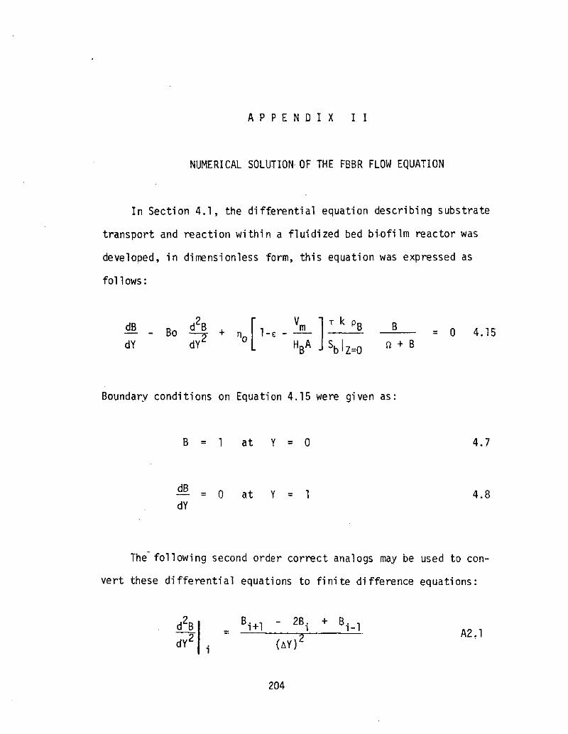
A P P E N D I X I I

NUMERICAL SOLUTION OF THE FEBR FLOW EQUATION

In Section 4.1, the differential equation describing substrate

transport and reaction within a fluidized bed bi-ofilm reactor was

developed, in dimensionless form, this equation, was expressed as

fol 1ows:

- BodY dY2 ^

[l. ^ 11 " t "

L HBA J

T k Pg

Sb Z=0

B

n + B= 0 4.15

Boundary conditions on Equation 4.15 were given as

B = 1 at Y = 0 4.7

dBdY

= 0 at Y = 1 4.8

The following second order correct analogs may be used to con-

vert these differential equations to finite difference equations:

A2.1d2B

dY2

Bi+l - 2Bi + Bi-l

i (AY)2

204

205

dB _ i+1 " i-1

dY i 2(AY)

Equation 4.15 may then be approximated as follows:

B _ 2B + B

2(AX)

Z=0 n + B. A2*3

A non-linearity is encountered in Equation A2.3 due to the

(ft + B.) term. This necessitates an iterative solution procedure in

which Equation A2.3 is linearized by replacing the dependent variableA

in this term B. with a trial value B.. Equation A2.3 can then beA

solved and the computed values B. compared with the trial values B..

If the comparison is unsatisfactory, the computed B. values are used*\

to replace the assumed B. values for the next trial solution. With

this linearization, Equation A2.3 may be rewritten as follows:

B.., = 0 A2.4

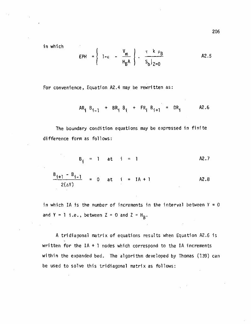
in which

EPH = l-E

Vm

HBA

T k pg

Sb Z=0

206

A2.5

For convenience, Equation A2.4 may be rewritten as:

AR. Bi-1 + BR. B1 A2.6

The boundary condition equations may be expressed in finite

difference form as follows:

Bi = 1 at i = 1 A2.7

2 ( A Y )= 0 at i = IA + 1 A2.8

in which IA is the number of increments in the interval between Y = 0

and Y = 1 i.e., between I = 0 and I = Hn.

A tridiagonal matrix of equations results when Equation A2.6 is

written for the IA + 1 nodes which correspond to the IA increments

within the expanded bed. The algorithm developed by Thomas (139) can

be used to solve this tridiagonal matrix as follows:

207

AR FRM

BBB. = BR, - — — with BBB, = BR9 A2.91 1 BBB._.j ^ *

thenOR. - AR.GGG. , DR9

GGG. = — - ]JLl With GGG9 = —£ A2.101 BBB. * BR2

The values of the dependent variable, dimensionless bulk-substrate

concentration, are then computed as follows:

A2.ll

B. = GGG. - j 1+] A2.121 1 BBB.

208

FBBR MODEL - COMPUTER PROGRAM NOMENCLATURE

DSL

RL

VIS

DSB

XK

XKS

Q

SO

XA

HB

RM

DM

VM

G

U

DEL

DP

XM, XB =

RB

RBW

RS

UT

DSL

PLn

DSE

k

KS

Q

sbA

HBPm

dmvm

9

U

5

dPC0€

PBPBIpsu.

coefficients in Eq. 4.17

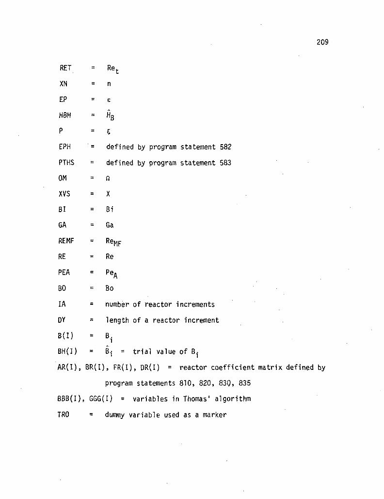
209

RET = Ret

XN = n

EP = e

HBH = HB

P = €

EPH = defined by program statement 582

PTHS = defined by program statement 583

OM = fl

XVS = X

BI = Bi

GA = Ga

REMF ~ ReMF

RE = Re

PEA = PeA

BO = Bo

IA = number of reactor increments

DY ~ length of a reactor increment

B(I) - B.

BH(I) = iij = trial value of B-

AR(I), BR(I), FR(I), DR(I) = reactor coefficient matrix defined by

program statements 810, 820, 830, 835

BBB(I), GGG(I) = variables in Thomas' algorithm

TRO = dummy variable used as a marker

210

EROK - allowable error

PER = fractional error

DS(I) = Z

TA(I) = T

TAU = T

N03-N = Nitrate-nitrogen concentration

ETA = n

IR = number of biofilm increments

DX = length of a biofilm increment

= C

CH(I) = Ci = trial value of Ci

GM(I) = YI

THS(I) = 4^2

AP(I), BP(I), FP(I), OP(I) = biofilm coefficient matrix defined by

program statements 2270, 2280, 2290, 2300

BB(I), GG(I) = variables in Thomas' algorithm

TOO = dummy variable used as a marker

PE = fractional error

ALER = allowable error

ET = differential effectiveness factor

211

10 PROGRAM FBBRdNPUT, OUTPUT)20 DIMENSION BU10) ,BHU10) , E T A ( 1 10), A R < 1 10),BR(1 10) ,

95C ftfttt COS UNITS USED THROUGHOUT100C ***LIQUID PHASE PARAMETERS ***110 DSL=t.67E-5120 RL=.998130 VIS=. 009548HOC *** BFILM PARAMETERS ***150 DSB=.815E-5160 XK=3.32E-5170 XKS=6.06E-8180C *** SYSTEM DEP PARAMETERS ***190 Q=11.4200 50=30, E-6210C *** REACTOR PARAMETERS ***220 XA=11.4230 HB=94.240C *** SUPPORT HEBIA PARAHETERS ***250 RM=2.42260 DM=6.32E-2270 VH=50.280C *************290 G=980.i2300 U=Q/XA310C flit ft BED FLUIIUZATION ALGORITHM HStt320 DEL-0.0325 325 CONTINUE330 DP=2.*DEUDM335C *** BIOFILM DENSITY-DEL CORRELATION ***340 IFdiEL.LE. 0.03)350, 380350 350 XM=0.0360 XB=.065370 GO TO 440380 380 IFtDEL.LE. 0.063)390, 420390 390 XM=-.035/.033400 XB=.096B410 GO TO 440420 420 XH=0.0430 XB=.03440 440 RB=XM*DEL+XB450 RBU=RL+RB/.8460 RS = RBU + (RH-RBW)*(DM/DP):**3470C *** PARTICLE TERMINAL VELOCITY ***480 UT = «RS-RL)*G*DP**(5./3.)/(27.5*RL**(1./3.>485+*VIS**(2./3.)))**(3./4.)490 RET=UT*RL*DP/V IS500C *** E X P A N S I O N INDEX CORRELAT ION ***510 X N = 1 0 . 3 5 * R E T * * ( - . 1 8 )

212

*** CALC HED VOIDAGE ***530 EP=<U/UT)**M./XN>540C *** CALC TRIAL BED HEIGHT ***550 HBH=VH/(XA*n.-EP»*<BP/DH)**3560 IF(HBH.LT.HB)565,580565 565 DEL=IiEL + 5.E-4570 GO TO 325580 580 CONTINUE581 P=DH/(2.*DEL)582 EPH=«1.-EP)-VH/(HB*XA))*OIB*XK*RB/(SO*U))583 PTHS=XK*RB*DEL**2/DSB594 OH=XKS/SO585C *** CALC REACTOR US ***590 XVS=VH*RB/(XA*HB)*((DP/BM)**3-1.)600 PRINT 610,DEL,PP,EP,XVS610 610 FQRMAT(4HBEL=,F10.5,/,3HDP=,F10.5,/,3HEP=,615+ F10.5,/,4HXVS=,F10,8,/)620C WttWtttiflW625C630C *** BIOT NUMBER CORRELATION ***635C *** BFILH EXTERNAL MASS TRANSFER **=c640 BI*(.81/EP)*(DSL/DSB)*(DEL/DP)*<U*RL*DP/VIS)**645+ (1./2.)*(VIS/(RL*DSL))**(1./3.)650 PRINT 660,BI660 660 FORHAT(3HBI=,F10,5,/)665C #ti38WttW##670C *** AXIAL DISPERSION CORRELATION ***680 GA=(RS-RL)'*RL*G*DP**3/VIS**2690C *** HIN.FLUID. REYNOLDS NO ***700 REMF=<33.7**2+.0408*GA)**(1./2.)-33.7710 RE=U*RL*DP/VIS720 PEA=REHF/(EP*RE)*(.2+.011*RE**(.48»722 BO=DP/(HB*PEA)725C 888 NUMBER OF REACTOR SEGMENTS = IA Hfttt730 IA=100735 IAP*IA+1737 IAM=IA-1740 DY=1./FLOAT(IA)745C filitJ DEFINE TRIAL PROFILE W747 B(1)=1.750 DO 770 IT=1,IAP760 BH(IT)=1.770 770 CONTINUE775 775 CONTINUE *780 CALL BFILH(BH,BI,SO,XKS,PTHS,P,IA,ETA)790C #88 DEFINE COEFFICIENT MATRIX W800 HO 840 1=1,IAP810 AR(I)=-1./(2.*DY)-BO/DY+*2820 BR(I)=2.*BO/BY**2+EPH*ETA(I)/(OH+BH(IJ)830 FR(I)=1./<2.*DY)-BO/DY**2835 DR(I)=0.0

213U40 840 CONTINUE850C $$* ENTRANCE BC $$*360 BR(2)=DR<2)-AR(2)870 AR(2)=0.0880C $$* EXIT BC $f*890 ARUAP) = AR(IAP)+FR(IAP)900 FR(IAP)=0.0910C BW«$ REACTOR THOMAS ALGORITHM H$tt$tf$920 BBB<2)=BR<2)930 GGG(2)=DR(2)/BR(2)940 DO 980 I=3,IAP950 IH=I-1960 BBB<I)=BR<I)-AR<I)*FR(Ifl)/BBB(IH)970 GGG(I) = (IiRa)-ARU)*GGG(IM»/BBB(I)980 980 CONTINUE990 B<IAP)*GGGtlHP)1000 DO 1030 JJJ=1,IAM1010 I=IAP-JJJ1015 IP=I+11020 B(I)=GGG(I)-FR(I)*B(IP)/BBB(IJ1030 1030 CONTINUEio4oc eeee COMPARE B s BH @0(?@1050 TRO=0.01060 EROK=.011070 DO 1120 1=2,IAP1080 PER=ABS((BHiI)-B(I))/B(D)1090 IF(PER.BT.EROK)t100,11101100 1100 TRO=1.1110 1 1 1 0 CONTINUE1 1 1 5 BH<I>=B(I)1120 1120 CONTINUE1130 IFURO.EG.DGO TO 7751140 BO 1160 1=1,IAF1142 IM=I-11144 DS(I)=DY+HB*FLOAT(IH)1146 TAU)=DStI)/U1150 B(I)=B(I)+SO1160 1160 CONTINUE1170 PRINT 11301180 1180 FDRHAT<7X,1HZ,HX,3HTAU,HX,5HN03-N,8X,3HETA,/)1200 PRINT 130Q,(E)SU>,TA<I}fB(I),ETA<I),I = t(IAP,5>1300 1300 FORMATMF15.7)1500 END2000 SUBROUTINE BFILH<BH,BI,SO,XKSfPTHS,PtIA(ETA>2015 DIMENSION CH(110) „AP(110),BP(110),FP(110)FDP(110),C(110),BB<110),GG(110)2017t,GH(110)fTHS(110),ETA(110),SH(1lO)2020 IR=1002030 IRP=IRt1204020502060 BX=1./FLOAT(IR)

214

2070 DO 2090 ICH=2,IRPP2080 CHUCH> = 1.2090 2090 CONTINUE2100 IAP=IA+12140 DO 2490 KR=1,IAP2150 GM(KR)=XKS/(BH(KR)*SO)2155 THS(KR)=PTHS/(BH(KR)*30)2UO 2t60 CONTINUE2U5C2170C *** DEFINE COEFFICIENT MATRIX ***2180 DO 2240 I=2,IRPP2190 X2=FLOAT(I-2>2200 APU) = 1./BX**2-1./<OX*<F+X2*BX)>2210 BP(I)s-2./DX**2-THS(KR)/(GM<KR)+CH(I»2220 FF'(I) = 1./BX**2-M./(DX*<P+X2*BX))2230 DP(I)=0.02240 2240 CONTINUE2250C2240C *+* BFILM EXTERIOR BC ***2270 AP(IRPP)=APURPP) + FPURPP)2280 BPURPP)*BP(IRPP)-2.*BX*BI*FPURPP)2290 BP(IRPP)=-FP(IRPP)*2.*BX*BI2300 FP(1RPP)=0.02310C2320C *** BFILM INTERIOR BC ***2330 FP(2)=FP(2)+AP<2)2340 AP(2)=0.02350C2360C SfiflH BFILH THOMAS ALGORITHM2370 BB<2)=BP<2)2380 GG(2)=DP(2)/BP(2)2390 DO 2430 I=3FIRPP2400 IM=I-12410 BB(I)=BP(I)-AP(I)*FP(IH)/BB(IH)2420 G6(I)=(DP(I)-AP(I)*6G(IM))/BB(I)2430 2430 CONTINUE2440 C(IRPP)=GG(IRPP)2450 DO 2490 JJJ=2,IRP2460 I=IR3P-JJJ2470 IP=I+12480 C(I)=GG(I)-FP(I)*C(IP)/BB(I)2490 2490 CONTINUE2500 T00=0.02510 DO 2570 I=2,IRPP2520 PE=ABS(CH(I)-C(I))/C(I)2530 ALER=0.0012540 IF(PE.GT.ALER)2550,25602550 2550 TQO = 1.2540 2560 CHU)=CU)2570 2570 CONTINUE2580 IF<TOO.EQ.1.)GO TO 2(60

215

2400 DO 2650 1=2, IRP2410 IP=I+12620 X2 = FLOATU-2)2630 X1=FLOAT(I-1)2640 ET*ET+(C(I)/(GM(KR)+C(I))+C(IP)/(GM(KR)+C(IP)))*((P+X2*DX)+(P+X1*1)X2645+»**22650 2650 CONTINUE

2670 2690 CONTINUE2695 RETURM2700 ENDREADY.

A P P E N D I X I I I

NUMERICAL SOLUTION FOR 8IOFILM EFFECTIVENESS; RECTANGULAR COORDINATES

In Section 5.1, the following differential equation for substrate

transport and Michaelis-Menten reaction within a rectangular biofilm

was developed:

= 0

dY2

The appropriate boundary conditions on Equation 5.2 are

S = S, at Y = 0 5.3D

dS— = 0 at Y = 6 5.4dY

Using second order correct finite difference analogs the above equations

may be rewritten as follows:

/ DSB- 1 + I - 5- : 1 Sn- +| |S, + 1=0

A3.1

216

217

S. = S. at i * 1 A3.2i b

= 0 at i = R + 1 A3.32(dY)

Equation A3.1 is made linear through introduction of the approximateA

term S^. See Appendix I for details of this approximation.

For convenience, Equation A3.1 was rewritten:

ADj Si_1 + 60^ S1 + FDi S^ = DDi A3.4

Equation A3.4 may then be written for the R+l nodes corresponding

to the R biofilm increments in 6. As in Appendix I, Thomas' algorithm

can then be used to solve the resultant tridiagonal matrix.

The substrate concentration profile, obtained as outlined above,

may then be used to compute the biofilm overall effectiveness factor

n0 defined in Section 5.1 as:

6 Sb

rJ

dY 5.5

which is approximated by the following difference equation:

A P P E N D I X I V

EXPERIMENTAL DATA

219

220

Table 1.

RPR - Experimental Data; Rotational Speed Study

RPM

50

50

50

100

TOO

150

5 PB T

(pm) (mgVS/1) °C

42

59

47

38

61

36

60.8

62.7

66.1

59.4

65.8

61.1

22

22

21.5

21.

21.5

21.5

pH

6.9

6.9

7.

6.9

6.8

6.8

Q sf sb

(ml/min) (mgNO^-N/l)

49.

52.3

51.3

48.6

49.4

49.1

98.8

101.3

102.1

98.4

97.3

100.2

96.1

97.6

99.

95.5

92.3

97.4

Table 2. 221

RDR - EXPERIMENTAL DATA

6

(vim)

3856

84

108

130

155198

255

315

44

49

68

97

112

137

140

177

210

270

308

PB PT T

(mgVS/cm3)(mgTS/cm3) °C

54.5

68.2

63.4

55.69.471.559.263.

53.665.759.868.372.460.154.163.563.853.657.

58.9

72.782.379.361.1

99.189.484.6 .70.

60.183.

73.284.391.574.166.879.179.468.

71.573,6

21.21.521.

22.

21.522.

23.

23.

21.

23.21.522.21.522.

22.

22.

21.

22.

21.522.

pH

6.97.

6.8

6.9

6.9

6.9

6.9

7.

6.9

6.9

6.9

7.

6.9

6.8

6.8

6.9

6.9

6.9

6.9

7.

Q Sf S,

(ml/nrin) (mgNO~-N/l)

51.447.850.350.951.251.449.

49,350.450.351.

49.345.249.154.349.148.254.352.

50.6

24.224.727.125.324.

28.126.325.427.

51.447.850.350.949,148.

52.851.152.647.348.

21.719.820.718.216.418.216.716.616.247.944.344.541. 440.739.741.939.

40.

36.933.5

222Table 2. continued

5

36

49

93

134

136

158

175

210

258

310

PB

61.1

68.

58.

65.1

63.4

54.3

59.7

62.

59.3

56.4

PT

76.2

84.

73.4

81.4

78.5

67.9

74.5

77.4

74.4

71.3

T

22.

21.

21.

22.

23.

22.

22.

21.5

21.5

22.

PH

6.9

6.9

6.8

6.8

6.8

7.

6.9

6.9

7.

7.

Q

49.1

50.6

52.3

48.3

48.4

51.3

47.6

50.8

49.

52.2

Sf

100i2

99.8

96.

102.3

101.4

96.8

103.1

98.

102.

97.5

Sb

97.4

95.7

89.7

91.3

90.5

86.6

89.7

82.4

83.

77.2

223

Table 3.

FBBR - Bed

40 vm

U (cm/sec)

.361

.440

.50

.566

.66

.76

.971.3

e

.609

.625

.640

.659

.670

.691

.720

.76

88 ym

U(cm/sec)

.35

..406

.463

.537

.635

.760

.908

1.13

e

.605

.607

.631

.651

.660

.690

.715

.740

Expansion

167 ytn

U (cm/sec)

.380

.43

.494

.60

.681

.779

.89

1.0

1.14

1.46

e

.56

.589

.598

.629

.641

.659

.673

.690

.714

.745

207 vim

U( cm/sec)

.30

.341

.391

.484

.579

.681

.770

.8811.08

e

.577

.604

.607

.641

.662

.687

.706

.730

.750

224

Table 3 Continued...

220 ym

U(cm/sec)

.376

.466

.571

.692

.781

.850

.939

1.13

e

.615

.635

.669

.680

.709

.710

.736

.759

268 ym

U( cm/sec)

.394

.460

.514

.618

.671

.760

.829

.960

1.11

e

.631

.654

.670

.680

.701

.719

.720

.755

.770

281 ym

U(cm/sec)

.336

.391

.438

.514

.619

.738

.845

.990

1.18

e

.581

.605

.620

.639

.661

.691

.708

.731

.76

318 ym

U( cm/sec)

.431

.475

.533

.615

.718

.790

.908

1.12

1.37

e

.619

.621

.642

.655

.688

.695

.720

.749

.780

225

Table 3 Continued. . .

344 ym

U(cm/sec)

.385

.424

.460

.539

.600

.679

.810

.922

1.04

e

.651

.677

.679

.705

.719

.740

.760

.791

.805

420 ym

U (cm/ sec)

.379

.405

.525

.610

.720

.822

.949

1.01

1.24

e

.619

.639

.661

.682

.686

,725

.740

.751

.79

547 ym

U(cm/sec)

.307

.332

.372

.426

.459

.520

.610

.738

.850

.938

1.27

e

.555

.56

.596

.600

.618

.635

.651

.688

.701

.719

.777

i~ r ^ ...561 ym

U(cm/sec)

.375

.313

.360

.431

.531

.672

.789

.890

.955

1.16

e

.595

.611

.621

.645

.675

.710

.724

.758

.762

.80

226

Table 3 Continued...

590 urn

U(cm/sec) e

.302

.361

.426

.506

.590

.681

.759

.861

.979

1.23

,637

.668

.679

.702

.729

.750

.768

.779

.801

.819

666 uni

U(cm/sec) e

.285

.316

.350

.416

.499

.560

.615

.719

.846

.975

1.23

.589

.611

.630

.638

.665

.679

.692

.710

.740

.759

.80

703 ym

U{ cm/sec)

.306

' .345

.406

.489

.570

.658

.779

.835

.94

1.19

£

.629

.639

.662

.700

.722

.750

.761

.779

.795

.839

812 um

U(cm/sec)

.284

.361

.402

.450

.522

.612

.690

.839

.980

1.14

e

.591

.600

.621

.669

.680

.705

.718

.759

.780

.818

227

Table 3 Continued.. .

858 ym

U (cm/sec)

.461

.512

.579

.671

.759

.890

1.09

e

.658

.660

.685

.702

.725

.750

.780

1005 ym

U(cm/sec)

.429

.482

.565

.674

.lit

.880

.975

E

.630

.655

.680

.712

.735

.750

.779

1089 ym

U (cm/sec)

.369

.418

.477

.561

.638

.710

.789

.965

e

.659

.661

.685

.710

.721

.739

.76

.785

1207 ym

U(cm/sec)

.416

.471

.541

.659

.732

.810

.9161.05

E

.655

.678

.691

.720

.734

.751

.762

.795

228

Table 4

Bioparticle Terminal Velocity

6

(microns)

40

83

167

207

220

268

281

318

344

420

547

561

590 •-

666

703

812

PB

(mq VS/cm3)

57.6

70.6

66.8

62.1

73.6

32.6

62.0

56.1

30.8

52.9

45.7

37.0

26.6

20.8

36.6

26.8

PT(mg TS/cm3)

71.8

88.0

84.0

77.2

91.4

41.1

77.5

71.1

38.8

66.3

57.3

46.0

33.7

26.4

45.8

33.5

ut

C cm/sec

6.17

5.15

5.41

4.75

5.02

4.87

4.16

4.50

3.24

4.23

4.12

3.67

3.09

3.45

3.03

2.89

229

Table 4 continued. . .

6

(microns)

858

1005

1039

1207

PB

(mg VS/crri3)

34.7

31.1

24.7

21.1

PT(mg TS/cm3)

43.6

38.9

31.2

26.0

Ut

(cm/sei

3.50

3.17

2.87

2.95

Settling column water temperature = 20°

230

Table 5

FBBR Experimental Data

6 = 40 microns

X = 5054 mg VS/1

U ~ 0.76 cm/sec

Influent pH = 6.8

Effluent pH = 7.8

Effluent Temp. = 22°C

T NO^-N

(sec) (mg/1)

0 22.6

21.7 17.9

50.0 12.3

78.3 7.1

106.6 3.3

134.9 1.1

180.3 0.9

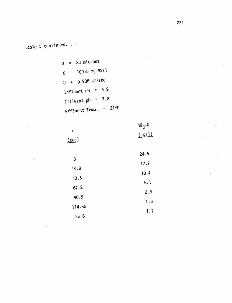
231

Table 5 continued. , .

5 = 88 microns

X = 10016 mg VS/1

U * Q.9Q8 cm/sec

Influent pH = 6.9

Effluent pH = 7-8

Effluent Temp* s 21°°

24.50

17.719.S

10.443.5

5.167.2

2.390.9

1.8114.55

1.1133.3

232

Table 5 continued. . .

6 = 167 microns

X = 15214 mg VS/1

U = 0.89 cm/sec

Influent pH = 6.9

Effluent pH = 7.9

Effluent Temp, = 22°C

T NOj-N

(sec) (mg/1)

0 30.5

19.7 22.0

43.8 . 13.5

67.95 7.4

92.1 3.6

110.6 2.0

233

Table 5 continued. . -

6 = 207 microns

x = 11784 mg VS/1

U = 1.07 cm/sec

Influent pH = 7*°

Eff luent pH s 7-6

Effluent Temp. * 22°c

21.00

17.815.75

13.936.61

10.756.53

8.076.46

6.196.39

4.4142.73

234

Table 5 continued. . .

6 = 220 microns

X = 16551 rng VS/1

U = 0.85 cm/sec

Influent pH = 6.8

Effluent pH = 7.8

Effluent Temp. = 19.5°C

i NO^-N

sec) (mg/1)

0 21.4

21.2 15.0

46.5 9.0

71.76 4.9

97.1 2.6

122.4 1.8

162.9 1.5

235

Table 5 continued. . .

6 = 268 microns

X = 6182 mg VS/1

U = 1.1 cm/sec

Influent pH = 6.9

Effluent pH = 7.4

Effluent Temp. = 21°C

T NO§-N

(sec) (mg/1)

0 21.8

17.3 17.6

36.8 14.9

56.4 12.6

75.9 9.9

95.5 7.6

108.2 6.8

236

Table 5 continued. . .

6 = 281 microns

X = 10357 mg VS/1

U = 1.59 cm/sec

Influent pH = 6.8

Effluent pH = 7.4

Effluent Temp. = 20°C

T

(sec) (mg/1)

0 21.3

11.7 18.6

25.2 16.0

38.7 13.3

52.3 11.2

65.8 9.7

72.7 8.9

237

Table 5 continued. . .

6 = 318 microns

X = 12307 mg VS/1

U = 1.03 cm/sec

Influent pH = 7.0

Effluent pH = 7,3

Effluent Temp. = 21°C

T NO^-N

'sec) . (mg/1)

0 22.1

17.1 17.4

38.5 12.7

58.9 9.3

79.9 6.4

91.6 4.8

238

Table 5 continued. . .

6 = 344 microns

X = 5400 mg VS/1

U = 1.0 cm/sec

Influent pH = 6.8

Effluent pH = 7.4

Effluent Temp. = 22°C

T NO^-N

'sec)

0 24.4

21.5 20.0

43.0 17.4

64.5 14.7

86.0 11.8

107.5 9.1

124.5 7.9

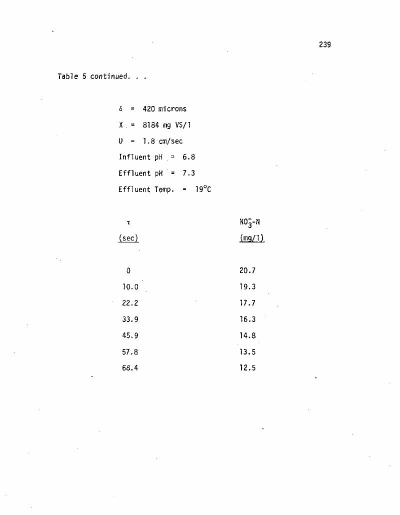
239

Table 5 continued. . .

6 = 420 microns

X . = 8184 mg VS/1

U = 1.8 cm/sec

Influent pH = 6.8

Effluent pH = 7.3

Effluent Temp. = 19°C

T NOg-N

(sec) (mg/1)

0 20.7

10.0 19.3

22.2 17.7

33.9 16.3

45.9 14.8

57.8 13.5

68.4 12.5

240

Table 5 continued. . .

6 = 547 microns

X = 10778 mg VS/1

U - 1.14 cm/sec

Influent pH = 7.0

Effluent pH = 7.6

Effluent Temp. = 22°C

T NO^-N

(sec)

0 16.0

16.7 13.5

35.5 10.9

54.4 8.5

73.2 6.6

92.1 5.0

119.3 3.9

241

Table 5 continued. . .

6 = 561 microns

X = 7875 mg VS/1

U = 1.04 cm/sec

Influent pH = 6.8

Effluent pH = 7.8

Effluent Temp. = 20°C

T NO^-N

(sec) (mg/l)

0 57.0

17.9 51.6

38.6 45.5

59.4 39.5

76.8 34.9

242

Table 5 continued. . .

6 = 590 microns

X = 5059 mg VS/1

U = 0.98 cm/sec

Influent pH = 6.9

Effluent pH = 7.7

Effluent Temp. = 22°C

NO^-N

(mg/1)

0 35.3

19.4 31.8

41.3 28.1

63.3 24.6

85.2 21.9

99.5 20.2

243

Table 5 continued. . .

6 = 666 microns

X = 6398 mg VS/1

U = 0.56 cm/sec

Influent pH = 7.0

Effluent pH = 7.6

Effluent Temp. = 20°C

T N03-N

sec) (mg/1)

0 27.1

33.1 22.3

71.5 16.1

109.9 11.5

148.3 8.6

136.7 6.8

206.4 6.2

244

Table 5 continued. . .

6 = 703 microns

X = 8125 mg VS/1

U = 0.82 cm/sec

Influent pH = 7.0

Effluent pH = 8.0

Effluent Temp. = 23°C

T N03-N

(sec) (mg/1)

0 30.1

20.8 25.0

47,2 18.7

73.5 13.6

99.9 9.5

126.3 6.5

133.6 5.5

245

Table 5 continued. . .

5 = 812 microns

X = 5744 mg VS/1

U = 0.98 cm/sec

Influent pH = 6.8

Effluent pH * 7.5

Effluent Temp. = 22°C

T NOg-N

\ '-sec)

0 24.1

17.4 21.4

39.3 18.6

61,2 16.4

83.2 14.5

105.0 12.8

151.0 10.8

246

Table 5 continued. . .

6 = 853 microns

X = 10171 mg VS/1

U = 0.67 cm/sec

Influent pH = 6.9

Effluent pH = 7.9

Effluent Temp. = 21°C

T NO^-N

(sec) (rng/1)

0 23.3

26.1 . 19.6

58.2 15.7

90.3 12.2

122.4 . 9.4

154.4 7.1

200.7 5.4

247

Table 5 continued. . .

6 - 1005 microns

X = 7649 mg VS/1

U = 0.88 cm/sec

Influent pH = 6.9

Effluent pH = 7.6

Effluent Temp. = 22°C

T NO~-N

(secj (mg/1)

0 19.2

19.3 16.7

43.8 13.9

68.2 11.3

92.6 9.0

117.1 7.0

134.1 5.9

248

Table 5 continued. . .

<5 = 1089 microns

X = 6091 mg VS/1

U - 0.76 cm/sec

Influent pH * 6.8

Effluent pH = 7.8

Effluent Temp. = 23°C

T NO§-N

(sec) (mg/1)

0 24.0

24.9 19.2

53.1 14.4

81.2 10.5

109.4 8.0

137.6 6.1

148.1 5.7

249

Table 5 continued. . .

6 = 1207 microns

X = 5845 mg VS/1

U = 0.66 cm/sec

Influent pH = 7.0

Effluent pH = 7.5

Effluent Temp. = 19°C

NOg-N

(mg/1)

0 18.3

28.0 15.8

60.6 13.3

93.2 11.0

125.8 8.7

158.4 7.2

203.2 5.4

Figures Al to A10. Comparisons of nitrate profiles, biomass holdupsand biofilm thicknesses observed in the laboratory FBBR and predictedby the FBBR model for each of the twenty experimental runs.

250

251

enE

1fO

28 -

r- 20 '

12 -

x(mgVS/l)

5054

7496

Observed

Predicted

10 210

28 -

20 -

12 '

x(mgVS/l)

88 10016

95 10146

Observed

— Predicted

10

Figure Al.

210

252

en

COoz: 12 '

4 -

50

Observed

Predicted

AM

167

150

x(mgVS/1)

15214

12756

90 130

i(sec)

170 210

Cn

I

fo

12 -

10

Figure A2.

50

6(u) x(mgVS/l)

Observed

Predicted

207

215

11784

13063

90 130 170 210

253

CDE

COo

COo

6(u) x(mgVS/l)

220 16551

?20 14626

Observed

Predicted

12

28 -

r 20 :

12

10

10

Figure A3.

50

210

6(u) x(mgVS/l)

•• Observed 268 6182

— Predicted 285 13619

90 130

i(sec)

170 210

28

20

roi 12

28

20

COo 12

10

10

50

50

• • Observed

— Predicted

6(u) x(mgVS/1)

281 10357

275 10472

90 130 170

t(sec)

210

• • Observed

— Predicted

6(u) x(mqVS/1)

318 12807

310 13967

90 130

t(sec)

170 210

254

Figure A4.

255

Observed

Predicted

344

400

x(mgVS/1)

5400

12418

210

28

enE

20

Observed

Predicted

420

400

x(mgVS/1)

8184

7685

12

Figure A5

50 90 130

r(sec)

170 210

28

20

Observed

Predicted

256

x(mgVS/1)

347 10778

510 8813

12

4 •

10 50 90

t(sec)

130 170 210

28

20cr

12

4 •

• • Observed

— Predicted

561

565

x(mgVS/l)

7875

7945

10

Figure A6.

50 90 130

T(SGC)

170 210

28

20

§ 12

28 -

20 -

o35 12

4 -

10 50

257

Observed

Predicted

g(u)

590

630

x(mgVS/l)

5059

6494

1

90 130

t(sec)

170 210

• • Observed

— Predicted

Figure A7.

28

20

sei

Observed

Predicted

703

745

258

x(mgVS/1)

8125

7557

_L10 50 90 130

t(sec)

170 210

28

20

5(u) x(mgV5/l)

•• Observed 812 5744

— Predicted 835 6831

ro12

10

Figure A8.

50 90 130

x(sec)

170 210

28

20

Observed

Predicted

259

858

350

x(mgVS/1)

10171

8629

12

4 -

50 90 130

r(sec)

170 210

28

en 20

x(mgVS/l)

Observed 1005 7649

Predicted 1035 7893

roO

12

10

Figure A9.

50 90 130

t(sec)

170 210

28

^ 20Dl

COO

12

10 50

Observed

Predicted

x(mgVS/1)

1089 6091

1185 9081

j.90

•r(sec)

130 170 210

260

28

o>

mo

20

12

.10

Figure A10.

50

x(mgVS/l)

•• Observed 1207 5845

— Predicted 1315 10189

x90 130

t(sec)

170 210