math 659: survival analysiswguo/math 659_2011/math659_chapter 2(2).pdf · wenge guo math 659:...

Math 659: Survival AnalysisChapter 2 — Basic Quantiles and Models (II)

Wenge Guo

July 22, 2011

Wenge Guo Math 659: Survival Analysis

Review of Last lecture (1)

I A lifetime or survival time is the time until some specifiedevent occurs. This event may be death, the appearance of atumor, the development of some disease, recurrence of adisease, equipment breakdown, cessation of breast feeding,and so on.

I Survival random variable: A random variable X is asurvival random variable if an observed outcome x of X isalways positive.

I Several functions characterize the distribution of a survivalrandom variable: probability density function (pdf) f (x),cumulative distribution function (cdf) F (x) survival function(sf) S(x), hazard function (hf) h(x), cumulative hazardfunction H(x), and mean residual lifetime mrl(x) at time x ,respectively.

Wenge Guo Chapter 2 Basic Quantities and Models

Review of Last lecture (2)

Implication of these functions:

I The survival function S(x) is the probability of an individualsurviving to time x .

I The hazard function h(x), sometimes termed risk function, isthe chance an individual of time x experiences the event inthe next instant in time when he has not experienced theevent at x .

I A related quantity to the hazard function is the cumulativehazard function H(x), which describes the overall risk ratefrom the onset to time x .

I The mean residual lifetime at age x , mrl(x), is the mean timeto the event of interest, given the event has not occurred at x .


Relationship Summary

We only need to know one of these functions, the rest can bederived. In particular,

I S(x) = 1− F (x),F (x) =∫ x0 f (t)dt,S(x) =

∫∞x f (t)dt

I f (x) = dF (x)dx = −dS(x)

dx

I h(x) = f (x)S(x) , H(x) =

∫ x0 h(t)dt, h(x) = dH(x)

dx

I mrl(x) =∫∞x (t−x)f (t)dt

S(x) =∫∞x S(t)dt

S(x) and

S(x) = mrl(0)mrl(x)e

−∫ x0

dtmrl(t)

I The key relation is S(x) = exp(−∫ x0 h(t)dt) = exp(−H(x)).


Discrete Case

I Suppose that X takes values xj , j = 1,2,3, · · ·I The probability mass function (pmf) p(xj) = Pr(X = xj),

j = 1,2, · · · where x1 < x2 < · · · < xj < · · ·I The survival function is defined as

S(x) = Pr(X > x) =∑

xj>x p(xj)

I Example: X with pmf p(xj) = Pr(X = j) = 1/3, j = 1,2,3,then the survival function is

S(x) = Pr(X > x) =∑xj>x

p(xj) =

1, 0 ≤ x < 1

2/3, 1 ≤ x < 21/3, 2 ≤ x < 3

0, x ≥ 3

18/33

Plot of the Survival Function for Discrete Case

19/33

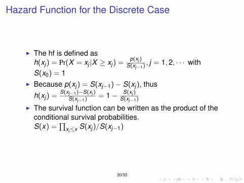
Hazard Function for the Discrete Case

I The hf is defined ash(xj) = Pr(X = xj |X ≥ xj) =

p(xj )S(xj−1) , j = 1,2, · · · with

S(x0) = 1I Because p(xj) = S(xj−1)− S(xj), thus

h(xj) =S(xj−1)−S(xj )

S(xj−1) = 1− S(xj )S(xj−1)

I The survival function can be written as the product of theconditional survival probabilities.S(x) =

∏xj≤x S(xj)/S(xj−1)

20/33

Relationship between h(xj) and S(x)

I Note that,

S(x) =Pr(X > x) = Pr(X > x |X > xj)Pr(X > xj)

=Pr(X > x |X > xj)Pr(X > xj |X > xj−1)Pr(X > xj−1)

= · · ·

I Because Pr(X > xj |X > xj−1) = S(xj)/S(xj−1)

I Thus S(x) =∏

xj≤x [1− h(xj)], which provides the basis forthe Kaplan-Meier estimator of the survival function

I The cumulative hazard function is defined asH(x) =

∑xj≤x h(xj)

I Note that S(x) = exp[−H(x)], which could be used toprovide an alternative estimator for the survival function

21/33

Relationship Summary for Discrete Lifetimes

Interrelationships between the various quantities for discretelifetimes X may be summarized as

I S(x) =∑

xj>x p(xj) =∏

xj≤x [1− h(xj)],

I p(xj) = S(xj)− S(xj−1) = h(xj)S(xj−1), j = 1, 2, . . . ,

I h(x) =p(xj )

S(xj−1),

I mrl(x) =(xi+1−x)S(xi )+

∑j≥i+1(xj+1−xj )S(xj )

S(x) , for xi ≤ x < xi+1.


Parametric Distributions

I We mainly use nonparametric and semiparametric modelsand methods in this class

I Parametric models are useful and widely used in somearea, such as reliability data analysis, engineer statistics

I The main purpose of survival analysis is to interpret data,for example, what is the population life distribution, what istreatment effect on the survival distribution, based on datacollected

I In reliability, often it is needed to make prediction for thefraction failing of a product after three year based onone-year data. Thus extrapolation is needed andparametric models are used

I In reliability, the use of parametric models can be justifiedby physical/chemical principles or engineering knowledge,but it is hard to make this justification for human body

22/33

The Exponential

I The sf is S(x) = exp(−λx), λ > 0, x ≥ 0I The pdf is f (x) = λexp(−λx)

I The hf is λI The mean and sd is 1/λI The lack of memory property, which means

Pr(X ≥ x + z|x ≥ x) = Pr(X ≥ z)

23/33

The Exponential (2)

Property: An important feature of the exponential distribution isthe ‘memoryless property’, P(X > x + z |X > x) = P(X > z).That is, on reaching any age, the probability of surviving z moreunits of time is the same as it was at age zero.

Example: For a component with an exponential distributedlifetime, the probability that a one-year-old component lasts 3more months in operation is the same as the probability that aten-year-old component lasts 3 more months in operations.

Implication: It indicates that the component’s lifetime does notpass through a period of ‘old ages’, where there is an increased riskof mortality.


The Exponential (3)

Application: The exponential probability model is one of the mostcommonly used probability models for modeling lifetimes ofcomponents. However, its constant hazard rate appears toorestrictive in health and some industrial applications.

Parameter: The parameter β is an important scale parameter, wehave the following conclusion: If X ∼ exp(λ), then λX ∼ exp(1).


The Weibull Distribution

I Widely used in reliabilityI The sf is S(x) = exp(−λxα)

I λ is a scale parameter and α is a shape parameterI The hf is λαxα−1, which is more flexible, allows different

shapes of the hazardI In particular, α determines the shape of the hazard

functionI α > 1, increasingI α = 1, constantI α < 1, decreasing

I Let Z = ln(λXα), then sf of Z is exp[−exp(z)], which iscalled the standard smallest extreme value distribution

24/33

The Weibull Hazard Function

25/33

Several Comments on Weibull Model

I The Weibull model has a very simple hazard function andsurvival function.

I It is a very useful model in many engineering context. Its twoparameters make the Weibull a very flexible model in a widevariety of situations: increasing hazards, decreasing hazards,and constant hazards.


Several Comments on Weibull Model (2)

I An understanding of the hazard rate may provide insight as towhat is causing the failures:

I A decreasing hazard rate would suggest ”infant mortality”.That is, defective items fail early and the failure rate decreasesover time as they fall out of the population.

I A constant hazard rate suggests that items are failing fromrandom events.

I An increasing hazard rate suggests ”wear out” - parts are morelikely to fail as time goes on.

I However, the mean and variance of the distribution are moredifficult to determine.


The Log Normal Distribution

Since many lifetimes are measured on the logarithm scale, andsuch transformations often increase the symmetry in data, it isimportant to examine the log normal distribution where thetransformed data are normally distributed.

A positive valued survival variable X has a log normal distributionand we write X ∼ lognormal(µ, σ) if Y = ln(X ) ∼ N(µ, σ).

Suppose Φ is the cumulative distribution function of the standardnormal random variable, the survival function ofX ∼ lognormal(µ, σ) is

S(x) = P(X > x) = P(ln(X ) > ln(x)) = 1− Φ(ln(x)− µ

σ),

from which the density and hazard may be obtained bydifferentiating S(x).


The Log Normal Distribution (2)

The features of the hazard rate: the hazard function of thelognormal is hump-shaped. It initially increases, reaches amaximum and then decreases toward 0 as lifetimes become largerand larger.

I The model is not suitable for lifetime modeling where hazardsincrease with old age.

I By using a part of the distribution, we can model the onset ofsome disease.

For the log normal distribution, the mean lifetime is given byexp(µ+ σ2) and the variance by [exp(σ2)− 1]exp(2µ+ σ2).


Lognormal Hazard Function

27/33

Log Logistic Distribution

Log-logistic distribution: mimic lognormal distributionproperties, but it has closed-form hazard and survival functions.

A positive valued survival variable X has a log logistic distributionand we write X ∼ loglogistic(µ, σ) with two parameters µ and σ ifY = ln(X ) follows a logistic distribution with survival function

SY (y) = 1− 1

1 + exp[−( y−µσ )].


Log Logistic Distribution (2)

The survival function of the log logistic distribution is

SX (x) = 1− 1

1 + exp[−( ln(x)−µσ )]=

1

1 + λxα,

where α = 1σ > 0 and λ = exp(−µ

σ ).

The hazard function is

hX (x) =αλxα

(1 + λxα)2,

which is similar in shape to the log normal hazard, but it isconsiderably easier to manipulate.


Regression Models

I To adjust the survival function to account for thecovariate/explanatory variables

I Examples:I Quantitative variables: blood pressure, temperature, age,

weightI Qualitative variables: gender, race, treatments, disease

statusI The explanatory variable is denoted z = (z1, · · · , zp)t

I Two approaches in regression:I Modeling Y = ln(X ), accelerated failure time modelI Modeling the hazard function h(x)

I Multiplicative hazard rate modelsI Additive hazard rate models

28/33

Accelerated Failure Time Model

I The first approach is analogous to the classical linearregression approach

I Y = ln(X ) = µ+ γtz + σW where γ is the regressioncoefficient vector, W is the error distribution

I If the error distribution is normal, then the regressionmodel is a lognormal

I If the error distribution is the smallest extreme valuedistribution, then the regression model is the Weibull

I This model is called accelerated failure time modelI Let S0(x) denote the sf of X when z = 0, then

S(x |z) = S0[x exp(−γtz)]I If exp(−γtz) > 1 the time scale is acceleratedI If exp(−γtz) < 1 the time scale is decelerated

29/33

Example

I Assume X is a Weibull distribution, Y = ln(X )

I The regression model is Y = γtz + σWI The sf under baseline is S0(x) = exp(−xα)

I The sf under z isS(x |z) = exp{−[x exp(−γtz)]α} = S0[x exp(−γtz)]

30/33

Multiplicative Hazard Model

I The Second approach is to model the hazard function as afunction of covariate

I The first class of model in this approach is called themultiplicative hazard rate model

I In particular, the conditional hazard rate of an individualwith covariate z is a product of the baseline hazard and anon-negative function of the covariate c(βtz), that ish(x |z) = h0(x)c(βtz)

I For Cox model, c(βtz) = exp(βtz)

I A key feature of this class of model is proportional hazardwhen z is fixed h(x |z1)

h(x |z2) = h0(x)c(βt z1)h0(x)c(βt z2)

= c(βt z1)c(βt z2)

I The sf under z is S(x |z) = S0(x)c(βt z)

31/33

Example

I Consider the baseline hazard to be a Weibull, that ish0(x) = αλxα−1

I h(x |z) = αλxα−1c(βtz)

I If Cox model is used h(x |z) = αλxα−1 exp(βtz)

I The sf under z isS(x |z) = exp[−λxα]exp(βt z) = exp[−λ(x exp[βtz/α])α]

I This is in the form of the accelerated failure time modelI The Weibull is the only continuous distribution which has

the property of being both an accelerated failure time anda multiplicative hazards model

32/33

Additive Hazard Model

I The second class of models for the hazard rate is thefamily of additive hazard rate model

I The condition hazard function is modeled by

h(x |z) = h0(x) +

p∑j=1

zj(x)βj(x)

I More details are in Chapter 10 (will not cover)

33/33

math 659: survival analysiswguo/math 659_2011/math659_chapter 2(2).pdf · wenge guo math 659:...

Documents