Math 407A: Linear Optimization

Lecture 8: Initialization and the Two Phase Simplex Algorithm

Math Dept, University of Washington

Lecture 8: Initialization and the Two Phase Simplex Algorithm (Math Dept, University of Washington)Math 407A: Linear Optimization 1 / 27

1 Initialization

2 The Auxilliary Problem

3 The Two Phase Simplex Algorithm

Lecture 8: Initialization and the Two Phase Simplex Algorithm (Math Dept, University of Washington)Math 407A: Linear Optimization 2 / 27

Initialization

We have shown that if we are given a feasible dictionary (tableau) for an LP, thenthe simplex algorithm will terminate finitely if it is employed with a anti-cyclingrule.

The anti-cycling rule need only be applied on degenerate pivots, since cycling canonly occur in the presence of degeneracy.

The simplex algorithm will terminate in one of two ways:

The LP is determined to be unbounded.

An optimal BFS is found.

We now address the question of how to determine an initial feasible dictionary(tableau).

Lecture 8: Initialization and the Two Phase Simplex Algorithm (Math Dept, University of Washington)Math 407A: Linear Optimization 3 / 27

Initialization

We have shown that if we are given a feasible dictionary (tableau) for an LP, thenthe simplex algorithm will terminate finitely if it is employed with a anti-cyclingrule.

The anti-cycling rule need only be applied on degenerate pivots, since cycling canonly occur in the presence of degeneracy.

The simplex algorithm will terminate in one of two ways:

The LP is determined to be unbounded.

An optimal BFS is found.

We now address the question of how to determine an initial feasible dictionary(tableau).

Lecture 8: Initialization and the Two Phase Simplex Algorithm (Math Dept, University of Washington)Math 407A: Linear Optimization 3 / 27

Initialization

We have shown that if we are given a feasible dictionary (tableau) for an LP, thenthe simplex algorithm will terminate finitely if it is employed with a anti-cyclingrule.

The anti-cycling rule need only be applied on degenerate pivots, since cycling canonly occur in the presence of degeneracy.

The simplex algorithm will terminate in one of two ways:

The LP is determined to be unbounded.

An optimal BFS is found.

We now address the question of how to determine an initial feasible dictionary(tableau).

Lecture 8: Initialization and the Two Phase Simplex Algorithm (Math Dept, University of Washington)Math 407A: Linear Optimization 3 / 27

Initialization

We have shown that if we are given a feasible dictionary (tableau) for an LP, thenthe simplex algorithm will terminate finitely if it is employed with a anti-cyclingrule.

The anti-cycling rule need only be applied on degenerate pivots, since cycling canonly occur in the presence of degeneracy.

The simplex algorithm will terminate in one of two ways:

The LP is determined to be unbounded.

An optimal BFS is found.

We now address the question of how to determine an initial feasible dictionary(tableau).

Lecture 8: Initialization and the Two Phase Simplex Algorithm (Math Dept, University of Washington)Math 407A: Linear Optimization 3 / 27

Initialization

We have shown that if we are given a feasible dictionary (tableau) for an LP, thenthe simplex algorithm will terminate finitely if it is employed with a anti-cyclingrule.

The anti-cycling rule need only be applied on degenerate pivots, since cycling canonly occur in the presence of degeneracy.

The simplex algorithm will terminate in one of two ways:

The LP is determined to be unbounded.

An optimal BFS is found.

We now address the question of how to determine an initial feasible dictionary(tableau).

Lecture 8: Initialization and the Two Phase Simplex Algorithm (Math Dept, University of Washington)Math 407A: Linear Optimization 3 / 27

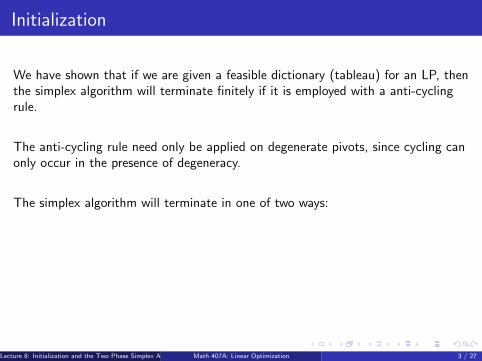
Initialization

We have shown that if we are given a feasible dictionary (tableau) for an LP, thenthe simplex algorithm will terminate finitely if it is employed with a anti-cyclingrule.

The anti-cycling rule need only be applied on degenerate pivots, since cycling canonly occur in the presence of degeneracy.

The simplex algorithm will terminate in one of two ways:

The LP is determined to be unbounded.

An optimal BFS is found.

We now address the question of how to determine an initial feasible dictionary(tableau).

Lecture 8: Initialization and the Two Phase Simplex Algorithm (Math Dept, University of Washington)Math 407A: Linear Optimization 3 / 27

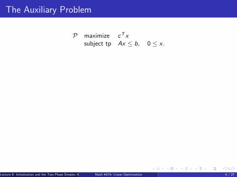
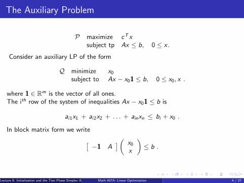
The Auxiliary Problem

P maximize cT xsubject tp Ax ≤ b, 0 ≤ x .

Consider an auxiliary LP of the form

Q minimize x0subject to Ax − x01 ≤ b, 0 ≤ x0, x .

where 1 ∈ Rm is the vector of all ones.The ith row of the system of inequalities Ax − x01 ≤ b is

ai1x1 + ai2x2 + . . . + ainxn ≤ bi + x0 .

In block matrix form we write[−1 A

]( x0x

)≤ b .

Lecture 8: Initialization and the Two Phase Simplex Algorithm (Math Dept, University of Washington)Math 407A: Linear Optimization 4 / 27

The Auxiliary Problem

P maximize cT xsubject tp Ax ≤ b, 0 ≤ x .

Consider an auxiliary LP of the form

Q minimize x0subject to Ax − x01 ≤ b, 0 ≤ x0, x .

where 1 ∈ Rm is the vector of all ones.

The ith row of the system of inequalities Ax − x01 ≤ b is

ai1x1 + ai2x2 + . . . + ainxn ≤ bi + x0 .

In block matrix form we write[−1 A

]( x0x

)≤ b .

Lecture 8: Initialization and the Two Phase Simplex Algorithm (Math Dept, University of Washington)Math 407A: Linear Optimization 4 / 27

The Auxiliary Problem

P maximize cT xsubject tp Ax ≤ b, 0 ≤ x .

Consider an auxiliary LP of the form

Q minimize x0subject to Ax − x01 ≤ b, 0 ≤ x0, x .

where 1 ∈ Rm is the vector of all ones.The ith row of the system of inequalities Ax − x01 ≤ b is

ai1x1 + ai2x2 + . . . + ainxn ≤ bi + x0 .

In block matrix form we write[−1 A

]( x0x

)≤ b .

Lecture 8: Initialization and the Two Phase Simplex Algorithm (Math Dept, University of Washington)Math 407A: Linear Optimization 4 / 27

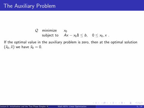
The Auxiliary Problem

P maximize cT xsubject tp Ax ≤ b, 0 ≤ x .

Consider an auxiliary LP of the form

Q minimize x0subject to Ax − x01 ≤ b, 0 ≤ x0, x .

where 1 ∈ Rm is the vector of all ones.The ith row of the system of inequalities Ax − x01 ≤ b is

ai1x1 + ai2x2 + . . . + ainxn ≤ bi + x0 .

In block matrix form we write[−1 A

]( x0x

)≤ b .

Lecture 8: Initialization and the Two Phase Simplex Algorithm (Math Dept, University of Washington)Math 407A: Linear Optimization 4 / 27

The Auxiliary Problem

Q minimize x0subject to Ax − x01 ≤ b, 0 ≤ x0, x .

If the optimal value in the auxiliary problem is zero, then at the optimal solution(x̃0, x̃) we have x̃0 = 0.

Plugging into Ax − x01 ≤ b, we get Ax̃ ≤ b, i.e. x̃ is feasible for P.

On the other hand, if x̂ is feasible for P, then (x̂0, x̂) with x̂0 = 0 is feasible for Q,so (x̂0, x̂) is optimal for Q.

Lecture 8: Initialization and the Two Phase Simplex Algorithm (Math Dept, University of Washington)Math 407A: Linear Optimization 5 / 27

The Auxiliary Problem

Q minimize x0subject to Ax − x01 ≤ b, 0 ≤ x0, x .

If the optimal value in the auxiliary problem is zero, then at the optimal solution(x̃0, x̃) we have x̃0 = 0.

Plugging into Ax − x01 ≤ b, we get Ax̃ ≤ b, i.e. x̃ is feasible for P.

On the other hand, if x̂ is feasible for P, then (x̂0, x̂) with x̂0 = 0 is feasible for Q,so (x̂0, x̂) is optimal for Q.

Lecture 8: Initialization and the Two Phase Simplex Algorithm (Math Dept, University of Washington)Math 407A: Linear Optimization 5 / 27

The Auxiliary Problem

Q minimize x0subject to Ax − x01 ≤ b, 0 ≤ x0, x .

If the optimal value in the auxiliary problem is zero, then at the optimal solution(x̃0, x̃) we have x̃0 = 0.

Plugging into Ax − x01 ≤ b, we get Ax̃ ≤ b, i.e. x̃ is feasible for P.

On the other hand, if x̂ is feasible for P, then (x̂0, x̂) with x̂0 = 0 is feasible for Q,so (x̂0, x̂) is optimal for Q.

Lecture 8: Initialization and the Two Phase Simplex Algorithm (Math Dept, University of Washington)Math 407A: Linear Optimization 5 / 27

The Auxiliary Problem

Q minimize x0subject to Ax − x01 ≤ b, 0 ≤ x0, x .

If the optimal value in the auxiliary problem is zero, then at the optimal solution(x̃0, x̃) we have x̃0 = 0.

Plugging into Ax − x01 ≤ b, we get Ax̃ ≤ b, i.e. x̃ is feasible for P.

On the other hand, if x̂ is feasible for P, then (x̂0, x̂) with x̂0 = 0 is feasible for Q,so (x̂0, x̂) is optimal for Q.

Lecture 8: Initialization and the Two Phase Simplex Algorithm (Math Dept, University of Washington)Math 407A: Linear Optimization 5 / 27

The Auxiliary Problem

P maximize cT xsubject tp Ax ≤ b,

0 ≤ x

Q minimize x0subject to Ax − x01 ≤ b,

0 ≤ x0, x

P is feasible ⇔ the optimal value in Q is zero.

P is infeasible ⇔ the optimal value in Q is positive.

Lecture 8: Initialization and the Two Phase Simplex Algorithm (Math Dept, University of Washington)Math 407A: Linear Optimization 6 / 27

The Auxiliary Problem

P maximize cT xsubject tp Ax ≤ b,

0 ≤ x

Q minimize x0subject to Ax − x01 ≤ b,

0 ≤ x0, x

P is feasible ⇔ the optimal value in Q is zero.

P is infeasible ⇔ the optimal value in Q is positive.

Lecture 8: Initialization and the Two Phase Simplex Algorithm (Math Dept, University of Washington)Math 407A: Linear Optimization 6 / 27

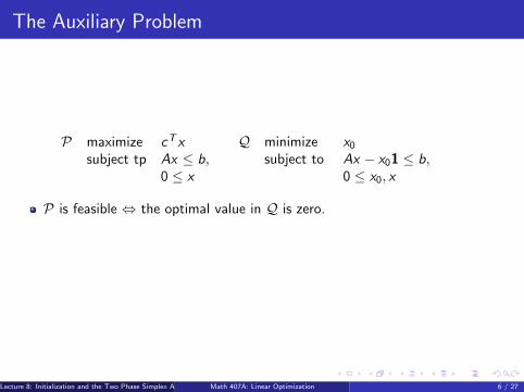
The Auxiliary Problem

P maximize cT xsubject tp Ax ≤ b,

0 ≤ x

Q minimize x0subject to Ax − x01 ≤ b,

0 ≤ x0, x

P is feasible ⇔ the optimal value in Q is zero.

P is infeasible ⇔ the optimal value in Q is positive.

Lecture 8: Initialization and the Two Phase Simplex Algorithm (Math Dept, University of Washington)Math 407A: Linear Optimization 6 / 27

Two Phase Simplex Algorithm

The auxiliary problem Q is also called the Phase I problem since solving it is thefirst phase of a two phase process of solving general LPs.

In Phase I we solve the auxiliary problem to obtain an initial feasible tableau forP, and in Phase II we solve the original LP starting with the feasible tableauprovided in Phase I.

Lecture 8: Initialization and the Two Phase Simplex Algorithm (Math Dept, University of Washington)Math 407A: Linear Optimization 7 / 27

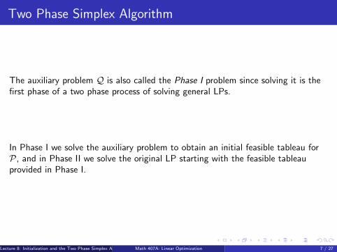
Two Phase Simplex Algorithm

The auxiliary problem Q is also called the Phase I problem since solving it is thefirst phase of a two phase process of solving general LPs.

In Phase I we solve the auxiliary problem to obtain an initial feasible tableau forP, and in Phase II we solve the original LP starting with the feasible tableauprovided in Phase I.

Lecture 8: Initialization and the Two Phase Simplex Algorithm (Math Dept, University of Washington)Math 407A: Linear Optimization 7 / 27

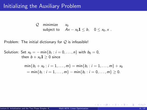
Initializing the Auxiliary Problem

Q minimize x0subject to Ax − x01 ≤ b, 0 ≤ x0, x .

Problem: The initial dictionary for Q is infeasible!

Solution: Set x0 = −min{bi : i = 0, . . . , n} with b0 = 0,then b + x01 ≥ 0 since

min{bi + x0 : i = 1, . . . ,m} = min{bi : i = 1, . . . ,m}+ x0

= min{bi : i = 1, . . . ,m} −min{bi : i = 0, . . . ,m} ≥ 0.

Hence, x0 = −min{bi : i = 0, . . . ,m} and x = 0 is feasible for Q.It is also a BFS for Q.

Lecture 8: Initialization and the Two Phase Simplex Algorithm (Math Dept, University of Washington)Math 407A: Linear Optimization 8 / 27

Initializing the Auxiliary Problem

Q minimize x0subject to Ax − x01 ≤ b, 0 ≤ x0, x .

Problem: The initial dictionary for Q is infeasible!

Solution: Set x0 = −min{bi : i = 0, . . . , n} with b0 = 0,then b + x01 ≥ 0 since

min{bi + x0 : i = 1, . . . ,m} = min{bi : i = 1, . . . ,m}+ x0

= min{bi : i = 1, . . . ,m} −min{bi : i = 0, . . . ,m} ≥ 0.

Hence, x0 = −min{bi : i = 0, . . . ,m} and x = 0 is feasible for Q.It is also a BFS for Q.

Lecture 8: Initialization and the Two Phase Simplex Algorithm (Math Dept, University of Washington)Math 407A: Linear Optimization 8 / 27

Initializing the Auxiliary Problem

Q minimize x0subject to Ax − x01 ≤ b, 0 ≤ x0, x .

Problem: The initial dictionary for Q is infeasible!

Solution: Set x0 = −min{bi : i = 0, . . . , n} with b0 = 0,then b + x01 ≥ 0 since

min{bi + x0 : i = 1, . . . ,m} = min{bi : i = 1, . . . ,m}+ x0

= min{bi : i = 1, . . . ,m} −min{bi : i = 0, . . . ,m} ≥ 0.

Hence, x0 = −min{bi : i = 0, . . . ,m} and x = 0 is feasible for Q.It is also a BFS for Q.

Lecture 8: Initialization and the Two Phase Simplex Algorithm (Math Dept, University of Washington)Math 407A: Linear Optimization 8 / 27

Initializing the Auxiliary Problem

Q minimize x0subject to Ax − x01 ≤ b, 0 ≤ x0, x .

Problem: The initial dictionary for Q is infeasible!

Solution: Set x0 = −min{bi : i = 0, . . . , n} with b0 = 0,then b + x01 ≥ 0 since

min{bi + x0 : i = 1, . . . ,m} = min{bi : i = 1, . . . ,m}+ x0

= min{bi : i = 1, . . . ,m} −min{bi : i = 0, . . . ,m} ≥ 0.

Hence, x0 = −min{bi : i = 0, . . . ,m} and x = 0 is feasible for Q.

It is also a BFS for Q.

Lecture 8: Initialization and the Two Phase Simplex Algorithm (Math Dept, University of Washington)Math 407A: Linear Optimization 8 / 27

Initializing the Auxiliary Problem

Q minimize x0subject to Ax − x01 ≤ b, 0 ≤ x0, x .

Problem: The initial dictionary for Q is infeasible!

Solution: Set x0 = −min{bi : i = 0, . . . , n} with b0 = 0,then b + x01 ≥ 0 since

min{bi + x0 : i = 1, . . . ,m} = min{bi : i = 1, . . . ,m}+ x0

= min{bi : i = 1, . . . ,m} −min{bi : i = 0, . . . ,m} ≥ 0.

Hence, x0 = −min{bi : i = 0, . . . ,m} and x = 0 is feasible for Q.It is also a BFS for Q.

Lecture 8: Initialization and the Two Phase Simplex Algorithm (Math Dept, University of Washington)Math 407A: Linear Optimization 8 / 27

Initializing the Auxiliary Problem

Q minimize x0subject to Ax − x01 ≤ b, 0 ≤ x0, x .

The initial dictionary for Q is

xn+i = bi + x0 −m∑j=1

aijxj

z = −x0.

Let i0 be such thatbi0 = min{bi : i = 0, 1, . . . ,m).

If i0 = 0, the LP has feasible origin and so the initial dictionary is optimal.

Lecture 8: Initialization and the Two Phase Simplex Algorithm (Math Dept, University of Washington)Math 407A: Linear Optimization 9 / 27

Initializing the Auxiliary Problem

Q minimize x0subject to Ax − x01 ≤ b, 0 ≤ x0, x .

The initial dictionary for Q is

xn+i = bi + x0 −m∑j=1

aijxj

z = −x0.

Let i0 be such thatbi0 = min{bi : i = 0, 1, . . . ,m).

If i0 = 0, the LP has feasible origin and so the initial dictionary is optimal.

Lecture 8: Initialization and the Two Phase Simplex Algorithm (Math Dept, University of Washington)Math 407A: Linear Optimization 9 / 27

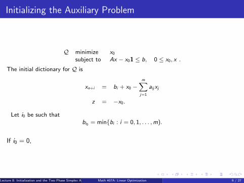
Initializing the Auxiliary Problem

Q minimize x0subject to Ax − x01 ≤ b, 0 ≤ x0, x .

The initial dictionary for Q is

xn+i = bi + x0 −m∑j=1

aijxj

z = −x0.

Let i0 be such thatbi0 = min{bi : i = 0, 1, . . . ,m).

If i0 = 0, the LP has feasible origin and so the initial dictionary is optimal.

Lecture 8: Initialization and the Two Phase Simplex Algorithm (Math Dept, University of Washington)Math 407A: Linear Optimization 9 / 27

Initializing the Auxiliary Problem

Q minimize x0subject to Ax − x01 ≤ b, 0 ≤ x0, x .

The initial dictionary for Q is

xn+i = bi + x0 −m∑j=1

aijxj

z = −x0.

Let i0 be such thatbi0 = min{bi : i = 0, 1, . . . ,m).

If i0 = 0,

the LP has feasible origin and so the initial dictionary is optimal.

Lecture 8: Initialization and the Two Phase Simplex Algorithm (Math Dept, University of Washington)Math 407A: Linear Optimization 9 / 27

Initializing the Auxiliary Problem

Q minimize x0subject to Ax − x01 ≤ b, 0 ≤ x0, x .

The initial dictionary for Q is

xn+i = bi + x0 −m∑j=1

aijxj

z = −x0.

Let i0 be such thatbi0 = min{bi : i = 0, 1, . . . ,m).

If i0 = 0, the LP has feasible origin and so the initial dictionary is optimal.

Lecture 8: Initialization and the Two Phase Simplex Algorithm (Math Dept, University of Washington)Math 407A: Linear Optimization 9 / 27

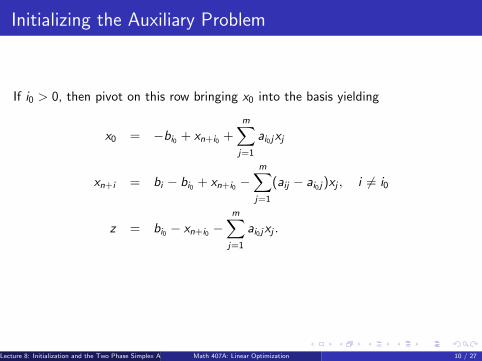
Initializing the Auxiliary Problem

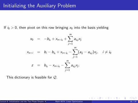
If i0 > 0, then pivot on this row bringing x0 into the basis yielding

x0 = −bi0 + xn+i0 +m∑j=1

ai0jxj

xn+i = bi − bi0 + xn+i0 −m∑j=1

(aij − ai0j)xj , i 6= i0

z = bi0 − xn+i0 −m∑j=1

ai0jxj .

This dictionary is feasible for Q.

Lecture 8: Initialization and the Two Phase Simplex Algorithm (Math Dept, University of Washington)Math 407A: Linear Optimization 10 / 27

Initializing the Auxiliary Problem

If i0 > 0, then pivot on this row bringing x0 into the basis yielding

x0 = −bi0 + xn+i0 +m∑j=1

ai0jxj

xn+i = bi − bi0 + xn+i0 −m∑j=1

(aij − ai0j)xj , i 6= i0

z = bi0 − xn+i0 −m∑j=1

ai0jxj .

This dictionary is feasible for Q.

Lecture 8: Initialization and the Two Phase Simplex Algorithm (Math Dept, University of Washington)Math 407A: Linear Optimization 10 / 27

Initializing the Auxiliary Problem: Example

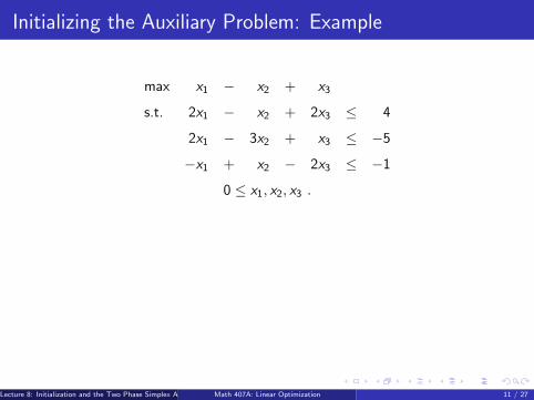
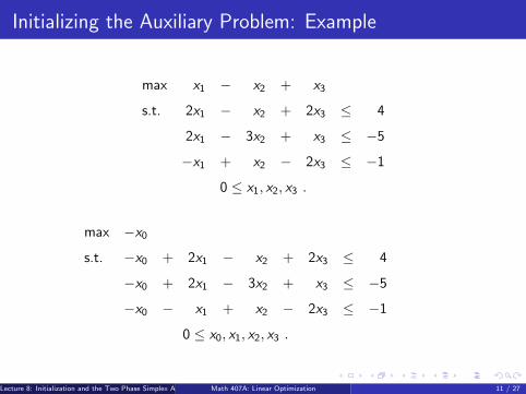
max x1 − x2 + x3

s.t. 2x1 − x2 + 2x3 ≤ 4

2x1 − 3x2 + x3 ≤ −5

−x1 + x2 − 2x3 ≤ −1

0 ≤ x1, x2, x3 .

max −x0s.t. −x0 + 2x1 − x2 + 2x3 ≤ 4

−x0 + 2x1 − 3x2 + x3 ≤ −5

−x0 − x1 + x2 − 2x3 ≤ −1

0 ≤ x0, x1, x2, x3 .

Lecture 8: Initialization and the Two Phase Simplex Algorithm (Math Dept, University of Washington)Math 407A: Linear Optimization 11 / 27

Initializing the Auxiliary Problem: Example

max x1 − x2 + x3

s.t. 2x1 − x2 + 2x3 ≤ 4

2x1 − 3x2 + x3 ≤ −5

−x1 + x2 − 2x3 ≤ −1

0 ≤ x1, x2, x3 .

max −x0s.t. −x0 + 2x1 − x2 + 2x3 ≤ 4

−x0 + 2x1 − 3x2 + x3 ≤ −5

−x0 − x1 + x2 − 2x3 ≤ −1

0 ≤ x0, x1, x2, x3 .

Lecture 8: Initialization and the Two Phase Simplex Algorithm (Math Dept, University of Washington)Math 407A: Linear Optimization 11 / 27

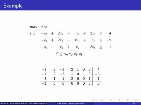
Example

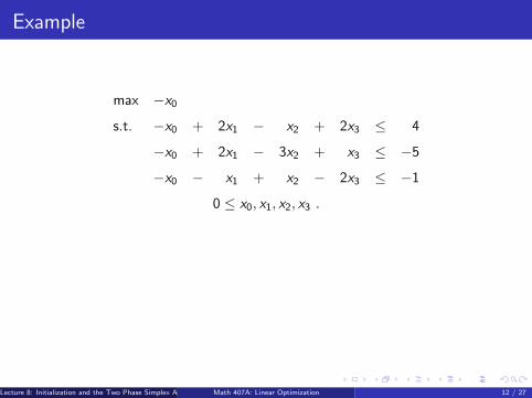
max −x0s.t. −x0 + 2x1 − x2 + 2x3 ≤ 4

−x0 + 2x1 − 3x2 + x3 ≤ −5

−x0 − x1 + x2 − 2x3 ≤ −1

0 ≤ x0, x1, x2, x3 .

−1 2 −1 2 1 0 0 4−1 2 −3 1 0 1 0 −5−1 −1 1 −2 0 0 1 −1−1 0 0 0 0 0 0 0

Lecture 8: Initialization and the Two Phase Simplex Algorithm (Math Dept, University of Washington)Math 407A: Linear Optimization 12 / 27

Example

max −x0s.t. −x0 + 2x1 − x2 + 2x3 ≤ 4

−x0 + 2x1 − 3x2 + x3 ≤ −5

−x0 − x1 + x2 − 2x3 ≤ −1

0 ≤ x0, x1, x2, x3 .

−1 2 −1 2 1 0 0 4−1 2 −3 1 0 1 0 −5−1 −1 1 −2 0 0 1 −1−1 0 0 0 0 0 0 0

Lecture 8: Initialization and the Two Phase Simplex Algorithm (Math Dept, University of Washington)Math 407A: Linear Optimization 12 / 27

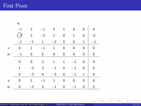
First Pivot

x0

−1 2 −1 2 1 0 0 4

−1 2 −3 1 0 1 0 -5

−1 −1 1 −2 0 0 1 −1

z 0 1 −1 1 0 0 0 0

w −1 0 0 0 0 0 0 0

0 0 2 1 1 −1 0 9

1 −2 3 −1 0 −1 0 5

0 −3 4© −3 0 −1 1 4

z 0 1 −1 1 0 0 0 0

w 0 −2 3 −1 0 −1 0 5

Lecture 8: Initialization and the Two Phase Simplex Algorithm (Math Dept, University of Washington)Math 407A: Linear Optimization 13 / 27

First Pivot

x0

−1 2 −1 2 1 0 0 4

−1© 2 −3 1 0 1 0 -5 most negative

−1 −1 1 −2 0 0 1 −1

z 0 1 −1 1 0 0 0 0

w −1 0 0 0 0 0 0 0

0 0 2 1 1 −1 0 9

1 −2 3 −1 0 −1 0 5

0 −3 4© −3 0 −1 1 4

z 0 1 −1 1 0 0 0 0

w 0 −2 3 −1 0 −1 0 5

Lecture 8: Initialization and the Two Phase Simplex Algorithm (Math Dept, University of Washington)Math 407A: Linear Optimization 14 / 27

First Pivot

x0

−1 2 −1 2 1 0 0 4

−1© 2 −3 1 0 1 0 -5

−1 −1 1 −2 0 0 1 −1

z 0 1 −1 1 0 0 0 0

w −1 0 0 0 0 0 0 0

0 0 2 1 1 −1 0 9

1 −2 3 −1 0 −1 0 5

0 −3 4 −3 0 −1 1 4

z 0 1 −1 1 0 0 0 0

w 0 −2 3 −1 0 −1 0 5

Lecture 8: Initialization and the Two Phase Simplex Algorithm (Math Dept, University of Washington)Math 407A: Linear Optimization 15 / 27

First Pivot

x0

−1 2 −1 2 1 0 0 4

−1 2 −3 1 0 1 0 -5

−1 −1 1 −2 0 0 1 −1

z 0 1 −1 1 0 0 0 0

w −1 0 0 0 0 0 0 0

0 0 2 1 1 −1 0 9

1 −2 3 −1 0 −1 0 5

0 −3 4© −3 0 −1 1 4

z 0 1 −1 1 0 0 0 0

w 0 −2 3 −1 0 −1 0 5

Lecture 8: Initialization and the Two Phase Simplex Algorithm (Math Dept, University of Washington)Math 407A: Linear Optimization 16 / 27

Second Pivot

0 0 2 1 1 −1 0 9

1 −2 3 −1 0 −1 0 5

0 −3 4© −3 0 −1 1 4

z 0 1 −1 1 0 0 0 0

w 0 −2 3 −1 0 −1 0 5

0 32

0 52

1 − 12

− 12

7

1 14

0 54

0 − 14

− 34

2

0 − 34

1 − 34

0 − 14

14

1

z 0 14

0 14

0 − 14

14

1

w 0 14

0 54

0 − 14

− 34

2

Lecture 8: Initialization and the Two Phase Simplex Algorithm (Math Dept, University of Washington)Math 407A: Linear Optimization 17 / 27

Second Pivot

0 0 2 1 1 −1 0 9

1 −2 3 −1 0 −1 0 5

0 −3 4© −3 0 −1 1 4

z 0 1 −1 1 0 0 0 0

w 0 −2 3 −1 0 −1 0 5

0 32

0 52

1 − 12

− 12

7

1 14

0 54

0 − 14

− 34

2

0 − 34

1 − 34

0 − 14

14

1

z 0 14

0 14

0 − 14

14

1

w 0 14

0 54

0 − 14

− 34

2

Lecture 8: Initialization and the Two Phase Simplex Algorithm (Math Dept, University of Washington)Math 407A: Linear Optimization 17 / 27

Second Pivot

0 0 2 1 1 −1 0 9

1 −2 3 −1 0 −1 0 5

0 −3 4© −3 0 −1 1 4

z 0 1 −1 1 0 0 0 0

w 0 −2 3 −1 0 −1 0 5

0 32

0 52

1 − 12

− 12

7

1 14

054© 0 − 1

4− 3

42

0 − 34

1 − 34

0 − 14

14

1

z 0 14

0 14

0 − 14

14

1

w 0 14

0 54

0 − 14

− 34

2

Lecture 8: Initialization and the Two Phase Simplex Algorithm (Math Dept, University of Washington)Math 407A: Linear Optimization 18 / 27

Third Pivot

0 32

0 52

1 − 12

− 12

7

1 14

054© 0 − 1

4− 3

42

0 − 34

1 − 34

0 − 14

14

1

z 0 14

0 14

0 − 14

14

1

w 0 14

0 54

0 − 14

− 34

2

−2 1 0 0 1 0 1 3

45

15

0 1 0 − 15

− 35

85

35

− 35

1 0 0 − 25

− 15

115

z − 15

420

0 0 0 − 420

820

35

w −1 0 0 0 0 0 0 0

Lecture 8: Initialization and the Two Phase Simplex Algorithm (Math Dept, University of Washington)Math 407A: Linear Optimization 19 / 27

Third Pivot

0 32

0 52

1 − 12

− 12

7

1 14

054© 0 − 1

4− 3

42

0 − 34

1 − 34

0 − 14

14

1

z 0 14

0 14

0 − 14

14

1

w 0 14

0 54

0 − 14

− 34

2

−2 1 0 0 1 0 1 3 Auxiliary

45

15

0 1 0 − 15

− 35

85

problem

35

− 35

1 0 0 − 25

− 15

115

solved.

z − 15

420

0 0 0 − 420

820

35

w −1 0 0 0 0 0 0 0

Lecture 8: Initialization and the Two Phase Simplex Algorithm (Math Dept, University of Washington)Math 407A: Linear Optimization 20 / 27

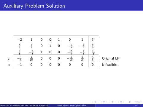
Auxiliary Problem Solution

−2 1 0 0 1 0 1 3

45

15

0 1 0 − 15

− 35

85

35

− 35

1 0 0 − 25

− 15

115

z − 15

420

0 0 0 − 420

820

35

Original LP

w −1 0 0 0 0 0 0 0 is feasible.

Lecture 8: Initialization and the Two Phase Simplex Algorithm (Math Dept, University of Washington)Math 407A: Linear Optimization 21 / 27

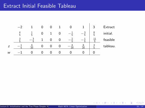
Extract Initial Feasible Tableau

−2 1 0 0 1 0 1 3 Extract

45

15

0 1 0 − 15

− 35

85

initial.

35

− 35

1 0 0 − 25

− 15

115

feasible

z − 15

420

0 0 0 − 420

820

35

tableau.

w −1 0 0 0 0 0 0 0

−2 1 0 0 1 0 1 3 Extract

45

15

0 1 0 − 15

− 35

85

initial.

35

− 35

1 0 0 − 25

− 15

115

feasible

z − 15

420

0 0 0 − 420

820

35

tableau.

w −1 0 0 0 0 0 0 0

Lecture 8: Initialization and the Two Phase Simplex Algorithm (Math Dept, University of Washington)Math 407A: Linear Optimization 22 / 27

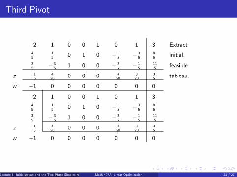
Third Pivot

−2 1 0 0 1 0 1 3 Extract

45

15

0 1 0 − 15

− 35

85

initial.

35

− 35

1 0 0 − 25

− 15

115

feasible

z − 15

420

0 0 0 − 420

820

35

tableau.

w −1 0 0 0 0 0 0 0

−2 1 0 0 1 0 1 3

45

15

0 1 0 − 15

− 35

85

35

− 35

1 0 0 − 25

− 15

115

z − 15

420

0 0 0 − 420

820

35

w −1 0 0 0 0 0 0 0

Lecture 8: Initialization and the Two Phase Simplex Algorithm (Math Dept, University of Washington)Math 407A: Linear Optimization 23 / 27

Phase II

1 0 0 1 0 1© 3

15

0 1 0 − 15

− 35

85

− 35

1 0 0 − 25

− 15

115

15

0 0 0 − 15

25

35

1 0 0 1 0 1 3

45

0 1 35

− 15

0 175

− 25

1 0 15

0 0 145

− 15

0 0 − 25

− 15

0 − 35

Lecture 8: Initialization and the Two Phase Simplex Algorithm (Math Dept, University of Washington)Math 407A: Linear Optimization 24 / 27

Phase II: Solution

1 0 0 1 0 1 3

45 0 1 3

5 − 15 0 17

5

− 25 1 0 1

5 0 0 145

− 15 0 0 − 2

5 − 15 0 − 3

5

Optimal primal and dual solutions are x1

x2

x3

=

0

2.8

3.4

y1

y2

y3

=

0.4

0.2

0

with optimal value z = .6.

Lecture 8: Initialization and the Two Phase Simplex Algorithm (Math Dept, University of Washington)Math 407A: Linear Optimization 25 / 27

Phase II: Solution

1 0 0 1 0 1 3

45 0 1 3

5 − 15 0 17

5

− 25 1 0 1

5 0 0 145

− 15 0 0 − 2

5 − 15 0 − 3

5

Optimal primal and dual solutions are

x1

x2

x3

=

0

2.8

3.4

y1

y2

y3

=

0.4

0.2

0

with optimal value z = .6.

Lecture 8: Initialization and the Two Phase Simplex Algorithm (Math Dept, University of Washington)Math 407A: Linear Optimization 25 / 27

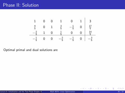
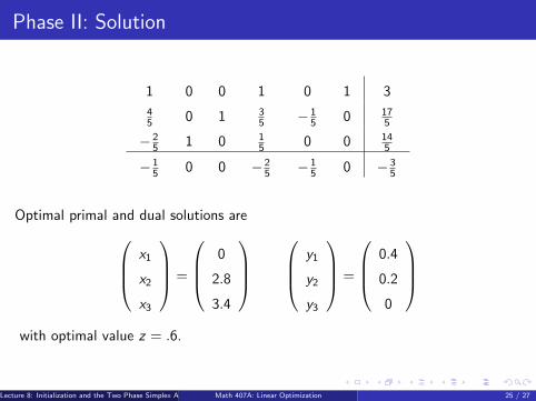
Phase II: Solution

1 0 0 1 0 1 3

45 0 1 3

5 − 15 0 17

5

− 25 1 0 1

5 0 0 145

− 15 0 0 − 2

5 − 15 0 − 3

5

Optimal primal and dual solutions are x1

x2

x3

=

0

2.8

3.4

y1

y2

y3

=

0.4

0.2

0

with optimal value z = .6.

Lecture 8: Initialization and the Two Phase Simplex Algorithm (Math Dept, University of Washington)Math 407A: Linear Optimization 25 / 27

Phase II: Solution

1 0 0 1 0 1 3

45 0 1 3

5 − 15 0 17

5

− 25 1 0 1

5 0 0 145

− 15 0 0 − 2

5 − 15 0 − 3

5

Optimal primal and dual solutions are x1

x2

x3

=

0

2.8

3.4

y1

y2

y3

=

0.4

0.2

0

with optimal value z = .6.

Lecture 8: Initialization and the Two Phase Simplex Algorithm (Math Dept, University of Washington)Math 407A: Linear Optimization 25 / 27

Phase II: Solution

1 0 0 1 0 1 3

45 0 1 3

5 − 15 0 17

5

− 25 1 0 1

5 0 0 145

− 15 0 0 − 2

5 − 15 0 − 3

5

Optimal primal and dual solutions are x1

x2

x3

=

0

2.8

3.4

y1

y2

y3

=

0.4

0.2

0

with optimal value z = .6.

Lecture 8: Initialization and the Two Phase Simplex Algorithm (Math Dept, University of Washington)Math 407A: Linear Optimization 25 / 27

Steps for Phase I of the Two Phase Simplex Algorithm

We assume bi0 = min{bi : i = 1, . . . ,m} < 0.

1 Form the standard initial tableau:

[0 A I b−1 c 0 0

].

2 Border the initial tableau:

−1 0 A I b0 −1 c 0 0−1 0 0 0 0

.

3 In the first pivot, the pivot row is the i0 row and the pivot column is the firstcolumn (the x0 column).

4 Apply simplex algorithm on the w row until optimality.

5 If optimal value is positive, stop the original LP is not feasible.

6 If the optimal value is zero, extract feasible tableau for the original problemand pivot to optimality.

Lecture 8: Initialization and the Two Phase Simplex Algorithm (Math Dept, University of Washington)Math 407A: Linear Optimization 26 / 27

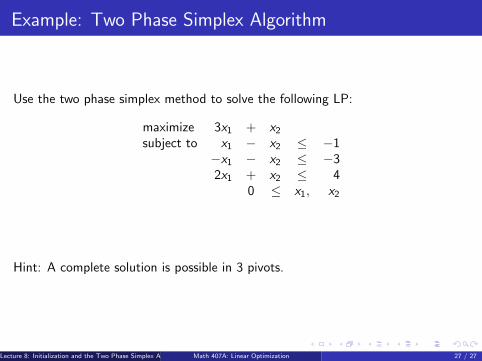
Example: Two Phase Simplex Algorithm

Use the two phase simplex method to solve the following LP:

maximize 3x1 + x2subject to x1 − x2 ≤ −1

−x1 − x2 ≤ −32x1 + x2 ≤ 4

0 ≤ x1, x2

Hint: A complete solution is possible in 3 pivots.

Lecture 8: Initialization and the Two Phase Simplex Algorithm (Math Dept, University of Washington)Math 407A: Linear Optimization 27 / 27