a parametric simplex algorithm for linear vector
TRANSCRIPT
A Parametric Simplex Algorithm for Linear Vector
Optimization Problems
Birgit Rudloff ∗ Firdevs Ulus † Robert Vanderbei ‡
April 20, 2016
Abstract
In this paper, a parametric simplex algorithm for solving linear vector optimization prob-lems (LVOPs) is presented. This algorithm can be seen as a variant of the multi-objectivesimplex (the Evans-Steuer) algorithm [15]. Different from it, the proposed algorithmworks in the parameter space and does not aim to find the set of all efficient solutions.Instead, it finds a solution in the sense of Lohne [19], that is, it finds a subset of efficientsolutions that allows to generate the whole efficient frontier. In that sense, it can also beseen as a generalization of the parametric self-dual simplex algorithm, which originallyis designed for solving single objective linear optimization problems, and is modified tosolve two objective bounded LVOPs with the positive orthant as the ordering cone inRuszczynski and Vanderbei [26]. The algorithm proposed here works for any dimension,any solid pointed polyhedral ordering cone C and for bounded as well as unboundedproblems.
Numerical results are provided to compare the proposed algorithm with an objectivespace based LVOP algorithm (Benson’s algorithm in [16]), that also provides a solution inthe sense of [19], and with the Evans-Steuer algorithm [15]. The results show that for non-degenerate problems the proposed algorithm outperforms Benson’s algorithm and is on parwith the Evan-Steuer algorithm. For highly degenerate problems Benson’s algorithm [16]outperforms the simplex-type algorithms; however, the parametric simplex algorithm isfor these problems computationally much more efficient than the Evans-Steuer algorithm.
Keywords: Linear vector optimization, multiple objective optimization, algorithms, pa-rameter space segmentation.
MSC 2010 Classification: 90C29, 90C05, 90-08
1 Introduction
Vector optimization problems have been studied for decades and many methods have beendeveloped to solve or approximately solve them. In particular, there are a variety of algorithmsto solve linear vector optimization problems (LVOPs).
∗Vienna University of Economics and Business, Institute for Statistics and Mathematics, Vienna 1020,Austria, [email protected].†Bilkent University, Department of Industrial Engineering, Ankara, 06800, Turkey, [email protected]‡Princeton University, Department of Operations Research and Financial Engineering, Princeton, NJ 08544,
USA, [email protected]
1
1.1 Related literature
Among the algorithms that can solve LVOPs, some are extensions of the simplex methodand are working in the variable space. In 1973, Evans and Steuer [15] developed a multi-objective simplex algorithm that finds the set of all ’efficient extreme solutions’ and the setof all ’unbounded efficient edges’ in the variable space, see also [11, Algorithm 7.1]. Later,some variants of this algorithm have been developed, see for instance [1, 2, 9, 10, 17, 32].More recently, Ehrgott, Puerto and Rodriguez-Chıa [13] developed a primal-dual simplexmethod that works in the parameter space. This algorithm does not guarantee to find the setof all efficient solutions, instead it provides a subset of efficient solutions that are enough togenerate the whole efficient frontier in case the problem is ’bounded’. All of these simplex-typealgorithms are designed to solve LVOPs with any number of objective functions where theordering is component-wise. Among these, the Evans-Steuer algorithm [15] is implementedas a software called ADBASE [30].
In [26], Ruszczynski and Vanderbei developed an algorithm to solve LVOPs with twoobjectives and the efficiency of this algorithm is equivalent to solving a single scalar linearprogram by the parametric simplex algorithm. Indeed, the algorithm is a modification of theparametric simplex method and it produces a subset of efficient solutions that generate thewhole efficient frontier in case the problem is bounded.
Apart from the algorithms that work in the variable or parameter space, there are al-gorithms working in the objective space. In [8], Dauer and Liu proposed a procedure todetermine the nondominated extreme points and edges of the image of the feasible region.Later, Benson [5] proposed an outer approximation algorithm that also works in the objectivespace. These methods are motivated by the observation that the dimension of the objectivespace is usually much smaller than the dimension of the variable space, and decision makerstend to choose a solution based on objective values rather than variable values, see for in-stance [7]. Lohne [19] introduced a solution concept for LVOPs that takes into account theseideas. Accordingly a solution consists of a set of ’point maximizers (efficient solutions)’ and aset of ’direction maximizers (unbounded efficient edges)’, which altogether generate the wholeefficient frontier. If a problem is ’unbounded’, then a solution needs to have a nonempty set ofdirection maximizers. There are several variants of Benson’s algorithm for LVOPs. Some ofthem can also solve unbounded problems as long as the image has at least one vertex, but onlyby using an additional Phase 1 algorithm, see for instance [19, Section 5.4]. The algorithmsprovided in [12, 19, 28, 29] solve in each iteration at least two LPs that are of the same sizeas the original problem. An improved variant where only one LP has to be solved in eachiteration has been proposed independently in [6] and [16]. In addition to solving (at least) oneLP, these algorithms solve a vertex enumeration problem in each iteration. As it can be seenin [6, 22, 23, 28], it is also possible to employ an online vertex enumeration method. In thiscase, instead of solving a vertex enumeration problem from the scratch in each iteration, thevertices are updated after an addition of a new inequality. Recently, Benson’s algorithm wasextended to approximately solve bounded convex vector optimization problems in [14, 21].
1.2 The proposed algorithm
In this paper, we develop a parametric simplex algorithm to solve LVOPs of any size andwith any solid pointed polyhedral ordering cone. Although the structure of the algorithm issimilar to the Evans-Steuer algorithm, it is different since the algorithm proposed here works
2

in the parameter space and it finds a solution in the sense that Lohne proposed in [19]. Inother words, instead of generating the set of all point and direction maximizers, it only finds asubset of them that already allows to generate the whole efficient frontier. More specifically,the difference can be seen at two points. First, in each iteration instead of performing apivot for each ’efficient nonbasic variable’, we perform a pivot only for a subset of them.This already decreases the total number of pivots performed throughout the algorithm. Inaddition, the method of finding this subset of efficient nonbasic variables is more efficientthan the method that is needed to find the whole set. Secondly, for an entering variable,instead of performing all possible pivots for all ’efficient basic variables’ as in [15], we performa single pivot by picking only one of them as the leaving variable. In this sense, the algorithmprovided here can also be seen as a generalization of the algorithm proposed by Ruszczynskiand Vanderbei [26] to unbounded LVOPs with more than two objectives and with moregeneral ordering cones.
In each iteration the algorithm provides a set of parameters which make the current vertexoptimal. This parameter set is given by a set of inequalities among which the redundant onesare eliminated. This is an easier procedure than the vertex enumeration problem, which isrequired in some objective space algorithms. Different from the objective space algorithms, thealgorithm provided here doesn’t require to solve an additional LP in each iteration. Moreover,the parametric simplex algorithm works also for unbounded problems even if the image hasno vertices and generates direction maximizers at no additional cost.
As in the scalar case, the efficiency of simplex-type algorithms is expected to be betterwhenever the problem is non-degenerate. In vector optimization problems, one may observedifferent types of redundancies if the problem is degenerate. The first one corresponds to the’primal degeneracy’ concept in scalar problems. In this case, a simplex-type algorithm mayfind the same ’efficient solution’ for many iterations. That is to say, one remains at the samevertex of the feasible region for more than one iteration. The second type of redundancycorresponds to the ’dual degeneracy’ concept in scalar problems. Accordingly, the algorithmmay find different ’efficient solutions’ which yield the same objective values. In other words,one remains at the same vertex of the image of the feasible region. Additionally to these, asimplex-type algorithm for LVOPs may find efficient solutions which yield objective valuesthat are not vertices of the image of the feasible region. Note that these points that are ona non-vertex face of the image set are not necessary to generate the whole efficient frontier.Thus, one can consider these solutions also as redundant.
The parametric simplex algorithm provided here may also find redundant solutions. How-ever, it will be shown that the algorithm terminates at a finite time, that is, there is norisk of cycling. Moreover, compared to the Evans-Steuer algorithm, the parametric simplexalgorithm finds much fewer redundant solutions in general.
We provide different initialization methods. One of the methods requires to solve twoLPs while a second method can be seen as a Phase 1 algorithm. Both of these methods workfor any LVOP. Depending on the structure of the problem, it is also possible to initialize thealgorithm without solving an LP or performing a Phase 1 algorithm.
This paper is structured as follows. Section 2 is dedicated to basic concepts and notation.In Section 3, the linear vector optimization problem and solution concepts are introduced. Theparametric simplex algorithm is provided in Section 4. Different methods of initialization areexplained in Section 4.8. Illustrative examples are given in Section 5. In Section 6, we comparethe parametric simplex algorithm provided here with the different simplex algorithms forsolving LVOPs that are available in the literature. Finally, some numerical results regarding
3

the efficiency of the proposed algorithm compared to Benson’s algorithm and the Evans-Steueralgorithm are provided in Section 7.
2 Preliminaries
For a set A ⊆ Rq, AC , intA, riA, clA, bdA, convA, coneA denote the complement, interior,relative interior, closure, boundary, convex hull, and conic hull of it, respectively. If A ⊆ Rqis a non-empty polyhedral convex set, it can be represented as
A = conv {x1, . . . , xs}+ cone {k1, . . . , kt}, (1)
where s ∈ N \ {0}, t ∈ N, each xi ∈ Rq is a point, and each kj ∈ Rq \ {0} is a direction ofA. Note that k ∈ Rq \ {0} is called a direction of A if A + {αk ∈ Rq| α > 0} ⊆ A. The setA∞ := cone {k1, . . . , kt} is the recession cone of A. The set of points {x1, . . . , xs} togetherwith the set of directions {k1, . . . , kt} are called the generators of the polyhedral convex setA. We say ({x1, . . . , xs}, {k1, . . . , kt}) is a V-representation of A whenever (1) holds. Forconvenience, we define cone ∅ = {0}.
A convex cone C is said to be non-trivial if {0} ( C ( Rq and pointed if it does notcontain any line. A non-trivial convex pointed cone C defines a partial ordering ≤C on Rq:
v ≤C w :⇔ w − v ∈ C.
For a non-trivial convex pointed cone C ⊆ Rq, a point y ∈ A is called a C-maximal elementof A if ({y}+ C \ {0}) ∩ A = ∅. If the cone C is solid, that is, if it has a non-emptyinterior, then a point y ∈ A is called weakly C-maximal if ({y}+ intC) ∩ A = ∅. The setof all (weakly) C-maximal elements of A is denoted by (w)MaxC (A). The set of (weakly)C-minimal elements is defined by (w)MinC (A) := (w)Max−C (A). The (positive) dual coneof C is the set C+ :=
{z ∈ Rq| ∀y ∈ C : zT y ≥ 0
}. The positive orthant of Rq is denoted by
Rq+, that is, Rq+ := {y ∈ Rq| yi ≥ 0, i = 1, . . . , q}.
3 Linear Vector Optimization Problems
We consider a linear vector optimization problem (LVOP) in the following form
maximize P Tx (with respect to ≤C) (P)
subject to Ax ≤ b,x ≥ 0,
where P ∈ Rn×q, A ∈ Rm×n, b ∈ Rm, and C ⊆ Rq is a solid polyhedral pointed orderingcone. We denote the feasible set by X := {x ∈ Rn| Ax ≤ b, x ≥ 0}. Throughout, we assumethat (P) is feasible, i.e., X 6= ∅. The image of the feasible set is defined as P T [X ] := {P Tx ∈Rq| x ∈ X}.
We consider the solution concept for LVOPs introduced by Lohne in [19]. To do so, letus recall the following. A point x ∈ X is said to be a (weak) maximizer for (P) if P T x is(weakly) C-maximal in P [X ]. The set of (weak) maximizers of (P) is denoted by (w)Max(P).
4

The homogeneous problem of (P) is given by
maximize P Tx (with respect to ≤C) (Ph)
subject to Ax ≤ 0,
x ≥ 0.
The feasible region of (Ph), namely X h := {x ∈ Rn| Ax ≤ 0, x ≥ 0}, satisfies X h = X∞, thatis, the non-zero points in X h are exactly the directions of X . A direction k ∈ Rn \ {0} ofX is called a (weak) maximizer for (P) if the corresponding point k ∈ X h \ {0} is a (weak)maximizer of the homogeneous problem (Ph).
Definition 3.1 ([16, 19]). A set X ⊆ X is called a set of feasible points for (P) and a setX h ⊆ X h \ {0} is called a set of feasible directions for (P).
A pair of sets(X , X h
)is called a finite supremizer for (P) if X is a non-empty finite set
of feasible points for (P), X h is a (not necessarily non-empty) finite set of feasible directionsfor (P), and
convP T [X ] + coneP T [X h]− C = P T [X ]− C. (2)
A finite supremizer (X , X h) of (P) is called a solution to (P) if it consists of only maxi-mizers.
The set P := P T [X ]−C is called the lower image of (P). Let y1, . . . , yt be the generatingvectors of the ordering cone C. Then, ({0} , {y1, . . . , yt}) is a V-representation of the cone C,that is, C = cone {y1, . . . , yt}. Clearly, if (X , X h) is a finite supremizer, then (P T [X ], P T [X h]∪{−y1, . . . ,−yt}) is a V-representation of the lower image P.
Definition 3.2. (P) is said to be bounded if there exists p ∈ Rq such that P ⊆ {p} − C.
Remark 3.3. Note that the recession cone of the lower image, P∞, is equal to the lowerimage of the homogeneous problem, that is, P∞ = P T [X h]−C, see [19, Lemma 4.61]. Clearly,P∞ ⊇ −C, which also implies P+
∞ ⊆ −C+. In particular, if (P) is bounded, then we haveP∞ = −C and X h = ∅.
The weighted sum scalarized problem for a parameter vector w ∈ C+ is
maximize wTP Tx (P1(w))
subject to Ax ≤ b,x ≥ 0,
and the following well known proposition holds.
Proposition 3.4 ([24, Theorem 2.5]). A point x ∈ X is a maximizer (weak maximizer)of (P) if and only if it is an optimal solution to (P1(w)) for some w ∈ intC+ (w ∈ C+ \{0}).
Proposition 3.4 suggests that if one could generate optimal solutions, whenever they exist,to the problems (P1(w)) for w ∈ intC+, then this set of optimal solutions X would be a set of(point) maximizers of (P). Indeed, it will be enough to solve problem (P1(w)) for w ∈ riW ,where
W := {w ∈ C+| wT c = 1}, (3)
5

for some fixed c ∈ intC. Note that (P1(w)) is not necessarily bounded for all w ∈ riW .Denote the set of all w ∈ riW such that (P1(w)) has an optimal solution by Wb. If one canfind a finite partition (W i
b )si=1 of Wb such that for each i ∈ {1, . . . , s} there exists xi ∈ X
which is an optimal solution to (P1(w)) for all w ∈ W ib , then, clearly, X = {x1, . . . , xs} will
satisfy (2) provided one can also generate a finite set of (direction) maximizers X h. Trivially,if problem (P) is bounded, then (P1(w)) can be solved optimally for all w ∈ C+, X h = ∅,and (X , ∅) satisfies (2). If problem (P) is unbounded, we will construct in Section 4 a set X hby adding certain directions to it whenever one encounters a set of weight vectors w ∈ C+
for which (P1(w)) cannot be solved optimally. The following proposition will be used toprove that this set X h, together with X = {x1, . . . , xs} will indeed satisfy (2). It providesa characterization of the recession cone of the lower image in terms of the weighted sumscalarized problems. More precisely, the negative of the dual of the recession cone of thelower image can be shown to consist of those w ∈ C+ for which (P1(w)) can be optimallysolved.
Proposition 3.5. The recession cone P∞ of the lower image satisfies
−P+∞ = {w ∈ C+| (P1(w)) is bounded}.
Proof. By Remark 3.3, we have P∞ = P T [X h]− C. Using 0 ∈ X h and 0 ∈ C, we obtain
−P+∞ = {w ∈ Rq| ∀xh ∈ X h, ∀c ∈ C : wT (P Txh − c) ≤ 0}
= {w ∈ C+| ∀xh ∈ X h : wTP Txh ≤ 0}. (4)
Let w ∈ −P+∞, and consider the weighted sum scalarized problem of (Ph) given by
maximize wTP Tx (Ph1(w))
subject to Ax ≤ 0,
x ≥ 0.
By (4), xh = 0 is an optimal solution, which implies by strong duality of the linear programthat there exist y∗ ∈ Rm with AT y∗ ≥ Pw and y∗ ≥ 0. Then, y∗ is also dual feasiblefor (P1(w)). By the weak duality theorem, (P1(w)) can not be unbounded.
For the reverse inclusion, let w ∈ C+ be such that (P1(w)) is bounded, or equivalently,an optimal solution exists for (P1(w)) as we assume X 6= ∅. By strong duality, the dualproblem of (P1(w)) has an optimal solution y∗, which is also dual feasible for (Ph1(w)). Byweak duality, (Ph1(w)) is bounded and has an optimal solution xh. Then, w ∈ −P+
∞ holds.Indeed, assuming the contrary, one can easily find a contradiction to the optimality of xh.
4 The Parametric Simplex Algorithm for LVOPs
In [15], Evans and Steuer proposed a simplex algortihm to solve linear multiobjective prob-lems. The algorithm moves from one vertex of the feasible region to another until it findsthe set of all extreme (point and direction) maximizers. In this paper we propose a para-metric simplex algorithm to solve LVOPs where the structure of the algortihm is similar tothe Evans-Steuer algorithm. Different from it, the parametric simplex algorithm provides asolution in the sense of Definition 3.1, that is, it finds subsets of extreme point and direction
6

maximizers that generate the lower image. This allows the algorithm to deal with the degen-erate problems more efficiently than the Evans-Steuer algorithm. More detailed comparisonof the two algorithms can be seen in Section 6.
In [26], Ruszczynski and Vanderbei generalize the parametric self dual method, whichoriginally is designed to solve scalar LPs [31], to solve two-objective bounded linear vectoroptimization problems. This is done by treating the second objective function as the auxilliaryfunction of the parametric self dual algorithm. The algorithm provided here can be seen asa generalization of the parametric simplex algortithm from biobjective bounded LVOPs toq-objective LVOPs (q ≥ 2) that are not necessarily bounded where we also allow for anarbitrary solid polyhedral pointed ordering cone C.
We first explain the algorithm for the problems that have a solution. One can keep inmind that the methods of initialization proposed in Section 4.8 will verify if the problem hasa solution or not.
Assumption 4.1. There exists a solution to problem (P).
This assumption is equivalent to having a nontrivial lower image P, that is, ∅ 6= P ( Rq.Clearly P 6= ∅ implies X 6= ∅, which is equivalent to our standing assumption. Moreover, byDefinition 3.1 and Proposition 3.4, Assumption 4.1 implies that there exist a maximizer whichguarantees that there exists some w0 ∈ intC+ such that problem (P1(w0)) has an optimalsolution. In Section 4.8, we will propose methods to find such a w0. It will be seen that thealgorithm provided here finds a solution if there exists one.
4.1 The Parameter set Λ
Throughout the algorithm we consider the scalarized problem (P1(w)) for w ∈ W where Wis given by (3) for some fixed c ∈ intC. As W is q − 1 dimensional, we will transform theparameter set W into a set Λ ⊆ Rq−1. Assume without loss of generality that cq = 1. Indeed,since C was assumed to be a solid cone, there exists some c ∈ intC such that either cq = 1or cq = −1. For cq = −1, one can consider problem (P) where C and P are replaced by −Cand −P .
Let c = (c1, . . . , cq−1)T ∈ Rq−1 and define the function w(λ) : Rq−1 → Rq and the setΛ ⊆ Rq−1 as follows:
w(λ) := (λ1, . . . , λq−1, 1− cTλ)T ,
Λ := {λ ∈ Rq−1| w(λ) ∈ C+}.
As we assume cq = 1, cTw(λ) = 1 holds for all λ ∈ Λ. Then, w(λ) ∈ W for all λ ∈ Λand for any w ∈ W , (w1, . . . , wq−1)T ∈ Λ. Moreover, if λ ∈ int Λ, then w(λ) ∈ riW andif w ∈ riW , then (w1, . . . , wq−1)T ∈ int Λ. Throughout the algorithm, we consider theparametrized problem
(Pλ) := (P1(w(λ)))
for some generic λ ∈ Rq−1.
4.2 Segmentation of Λ: Dictionaries and their optimality region
We will use the terminology for the simplex algorithm as it is used in [31]. First, we introduce
7

slack variables [xn+1, . . . , xn+m]T to obtain x ∈ Rn+m and rewrite (Pλ) as follows
maximize w(λ)T [P T 0]x (Pλ)
subject to [A I]x = b,
x ≥ 0,
where I is the identity and 0 is the zero matrix, all in the correct sizes. We consider a partitionof the variable indices {1, 2, . . . , n+m} into two sets B and N . Variables xj , j ∈ B, are called
basic variables and xj , j ∈ N , are called nonbasic variables. We write x =[xTB xTN
]Tand
permute the columns of [A I] to obtain[B N
]satisfying [A I]x = BxB + NxN , where
B ∈ Rm×m and N ∈ Rm×n. Similarly, we form matrices PB ∈ Rm×q, and PN ∈ Rn×q suchthat [P T 0]x = P TB xB + P TNxN . In order to keep the notation simple, instead of writing[P T 0]x we will occasionally write P Tx, where x stands then for the original decision variablein Rn without the slack variables.
Whenever B is nonsingular, xB can be written in terms of the nonbasic variables asxB = B−1b−B−1NxN . Then, the objective function of (Pλ) is
w(λ)T [P T 0]x = w(λ)T ξ(λ)− w(λ)TZTNxN ,
where ξ(λ) = P TB B−1b and ZN = (B−1N)TPB − PN .
We say that each choice of basic and nonbasic variables defines a unique dictionary.Denote the dictionary defined by B and N by D. The basic solution that corresponds to D isobtained by setting xN = 0. In this case, the values of the basic variables become B−1b. Boththe dictionary and the basic solution corresponding to this dictionary are said to be primalfeasible if B−1b ≥ 0. Moreover, if w(λ)TZTN ≥ 0, then we say that the dictionary D and thecorresponding basic solution are dual feasible. We call a dictionary and the correspondingbasic solution optimal if they are both primal and dual feasible.
For j ∈ N , introduce the halfspace
IDj := {λ ∈ Rq−1| w(λ)TZTN ej ≥ 0},
where ej ∈ Rn denotes the unit column vector with the entry corresponding to the variablexj being 1. Note that if D is known to be primal feasible, then D is optimal for λ ∈ ΛD,where
ΛD :=⋂j∈N
IDj .
The set ΛD ∩ Λ is said to be the optimality region of dictionary D.Proposition 3.4 already shows that a basic solution corresponding to a dictionary yields
a (weak) maximizer of (P). Throughout the algorithm we will move from dictionary todictionary and collect their basic solutions into a set X . We will later show that this set willbe part of the solution (X , X h) of (P). The algorithm will yield a partition of the parameterset Λ into optimality regions of dictionaries and regions where (Pλ) is unbounded. The nextsubsections explain how to move from one dictionary to another and how to detect and dealwith unbounded problems.
8

4.3 The set JD of entering variables
We call (IDj )j∈JD a defining (non-redundant) collection of half-spaces of the optimality region
ΛD ∩ Λ if JD ⊆ N satisfies
ΛD ∩ Λ =⋂j∈JD
IDj ∩ Λ and
ΛD ∩ Λ (⋂j∈J
IDj ∩ Λ, for any J ( JD.(5)
For a dictionary D, any nonbasic variable xj , j ∈ JD, is a candidate entering variable. Let uscall the set JD an index set of entering variables for dictionary D.
For each dictionary throughout the algorithm, an index set of entering variables is found.This can be done e.g. by the following two methods. Firstly, using the duality of polytopes, theproblem of finding defining inequalities can be transformed to the problem of finding a convexhull of given points. Then, the algorithms developed for this matter, see for instance [3], canbe employed. Secondly, in order to check if j ∈ N corresponds to a defining or a redundantinequality one can consider the following linear program in λ ∈ Rq−1
maximize w(λ)TZTN ej
subject to w(λ)TZTN ej ≥ 0, for all j ∈ N \ ({j} ∪ J redun),
w(λ)TY ≥ 0,
where J redun is the index set of redundant inequalities that have been already found andY = [y1, . . . , yt] is the matrix where y1, . . . , yt are the generating vectors of the ordering coneC. The inequality corresponding to the nonbasic variable xj is redundant if and only if theoptimal solution to this problem yields w(λ∗)TZTN e
j ≤ 0. In this case, we add j to the setJ redun. Otherwise, it is a defining inequality for the region ΛD ∩ Λ and we add j to the setJD. The set JD is obtained by solving this linear program successively for each untestedinequality against the remaining.
Remark 4.2. For the numerical examples provided in Section 5, the second method is em-ployed. Note that the number of variables for each linear program is q − 1, which is muchsmaller than the number of variables n of the original problem in general. Therefore, eachlinear program can be solved accurately and fast. Thus, this is a reliable and sufficientlyefficient method to find JD.
Before applying one of these methods, one can also employ a modified Fourier-Motzkinelimination algorithm as described in [4] in order to decrease the number of redundant in-equalities. Note that this algorithm has a worst-case complexity of O(2q−1(q− 1)2)n2). Eventhough it doesn’t guarantee to detect all of the redundant inequalities, it decresases thenumber significantly.
Note that different methods may yield a different collection of indices as the set JD mightnot be uniquely defined. However, the proposed algorithm works with any choice of JD.
4.4 Pivoting
In order to initialize the algorithm one needs to find a dictionary D0 for the parametrizedproblem (Pλ) such that the optimality region of D0 satisfies ΛD
0 ∩ int Λ 6= ∅. Note that the
9

existence of D0 is guaranteed by Assumption 4.1 and by Proposition 3.4. There are differentmethods to find an initial dictionary and these will be discussed in Section 4.8. For now,assume that D0 is given. By Proposition 3.4, the basic solution x0 corresponding to D0 is amaximizer to (P). As part of the initialization, we find an index set of entering variables JD
0
as defined by (5).Throughout the algorithm, for each dictionary D with given basic variables B, optimality
region ΛD∩Λ, and index set of entering variables JD, we select an entering variable xj , j ∈ JD,and pick analog to the standard simplex method a leaving variable xi satisfying
i ∈ arg mini ∈ B
(B−1N)ij > 0
(B−1b)i(B−1N)ij
, (6)
whenever there exists some i with (B−1N)ij > 0. Here, indices i, j are written on behalf of theentries that correspond to the basic variable xi and the nonbasic variable xj , respectively. Notethat this rule of picking leaving variables, together with the initialization of the algorithm witha primal feasible dictionary D0, guarantees that each dictionary throughout the algorithm isprimal feasible.
If there exists a basic variable xi with (B−1N)ij > 0 satisfying (6), we perform the pivotxj ↔ xi to form the dictionary D with basic variables B = (B∪{j})\{i} and nonbasic variables
N = (N∪{i})\{j}. For dictionary D, we have IDi = cl (IDj )C = {λ ∈ Rq−1| w(λ)TZTN ej ≤ 0}.
If dictionary D is considered at some point in the algorithm, it is known that the pivotxi ↔ xj will yield the dictionary D considered above. Thus, we call (i, j) an explored pivot
(or direction) for D. We denote the set of all explored pivots of dictionary D by ED.
4.5 Detecting unbounded problems and constructing the set X h
Now, consider the case where there is no candidate leaving variable for an entering variablexj , j ∈ JD, of dictionary D, that is, (B−1Nej) ≤ 0. As one can not perform a pivot, it is notpossible to go beyond the halfspace IDj . Indeed, the parametrized problem (Pλ) is unbounded
for λ /∈ IDj . The following proposition shows that in that case, a direction of the recessioncone of the lower image can be found from the current dictionary D, see Remark 3.3.
Proposition 4.3. Let D be a dictionary with basic and nonbasic variables B and N , ΛD ∩Λbe its optimality region satisfying ΛD∩ int Λ 6= ∅, and JD be an index set of entering variables.If for some j ∈ JD, (B−1Nej) ≤ 0, then the direction xh defined by setting xhB = −B−1Nej
and xhN = ej is a maximizer to (P) and P Txh = −ZTN ej.
Proof. Assume (B−1Nej) ≤ 0 for j ∈ JD and define xh by setting xhB = −B−1Nej andxhN = ej . By definition, the direction xh would be a maximizer for (P) if and only if it is a(point) maximizer for the homogeneous problem (Ph), see section 3. It holds
[A I]xh = BxhB +NxhN = 0.
Moreover, xhN = ej ≥ 0 and xhB = −B−1Nej ≥ 0 by assumption. Thus, xh is primal feasiblefor problem (Ph) and also for problem (Ph1(w(λ))) for all λ ∈ Λ, that is, xh ∈ X h \ {0}.Let λ ∈ ΛD ∩ int Λ, which implies w(λ) ∈ riW ⊆ intC+. Note that by definition of theoptimality region, it is true that w(λ)TZTN ≥ 0. Thus, xh is also dual feasible for (Ph1(w(λ))),
10

it is an optimal solution for the parametrized homogeneous problem for λ ∈ ΛD ∩ int Λ. ByProposition 3.4 (applied to (Ph) and (Ph1(w(λ)))), xh is a maximizer of (Ph). The value ofthe objective function of (Ph) at xh is given by
[P T 0]xh = P TB xhB + P TNx
hN = −ZTN ej .
Remark 4.4. If for an entering variable xj , j ∈ JD, of dictionary D, there is no candidateleaving variable, we conclude that problem (P) is unbounded in the sense of Definition 3.2.Then, in addition to the set of point maximizers X one also needs to find the set of (direction)maximizers X h of (P), which by Proposition 4.3 can be obtained by collecting directions xh
defined by xhB = −B−1Nej and xhN = ej for every j ∈ JD with B−1Nej ≤ 0 for all dictionariesvisited throughout the algorithm. For an index set JD of entering variables of each dictionaryD, we denote the set of indices of entering variables with no candidate leaving variable fordictionary D by JDb := {j ∈ JD| B−1Nej ≤ 0}. In other words, JDb ⊆ JD is such that forany j ∈ JDb , (Pλ) is unbounded for λ /∈ IDj .
4.6 Partition of Λ: putting it all together
We have seen in the last subsections that basic solutions of dictionaries yield (weak) pointmaximizers of (P) and partitions Λ into optimality regions for bounded problems (Pλ), whileencountering an entering variable with no leaving variable in a dictionary yields directionmaximizers of (P) as well as regions of Λ corresponding to unbounded problems (Pλ). Thiswill be the basic idea to construct the two sets X and X h and to obtain a partition of theparameter set Λ. In order to show that (X , X h) produces a solution to (P), one still needs toensure finiteness of the procedure, that the whole set Λ is covered, and that the basic solutionsof dictionaries visited yield not only weak point maximizers of (P), but point maximizers.
Observe that whenever xj , j ∈ JD, is the entering variable for dictionary D with ΛD∩Λ 6=∅ and there exists a leaving variable xi, the optimality region ΛD for dictionary D after thepivot is guaranteed to be non-empty. Indeed, it is easy to show that
∅ ( ΛD ∩ ΛD ⊆ {λ ∈ Rq−1| w(λ)TZN ej = 0},
where N is the collection of nonbasic variables of dictionary D. Moreover, the basic solutionsread from dictionaries D and D are both optimal solutions to the parametrized problem (Pλ)for λ ∈ ΛD ∩ ΛD. Note that the common optimality region of the two dictionaries has nointerior.
Remark 4.5. a. In some cases it is possible that ΛD itself has no interior and it is a subsetof the neighbouring optimality regions corresponding to some other dictionaries.
b. Even though it is possible to come across dictionaries with optimality regions having emptyinterior, for any dictionary D found during the algorithm ΛD ∩ int Λ 6= ∅ holds. This isguaranteed by starting with a dictionary D0 satisfying ΛD
0 ∩ int Λ 6= ∅ together withthe rule of selecting the entering variables, see (5). More specifically, throughout thealgorithm, whenever IDj corresponds to the boundary of Λ it is guaranteed that j /∈ JD.By this observation and by Proposition 3.4, it is clear that the basic solution correspondingto the dictionary D is not only a weak maximizer but it is a maximizer.
11

Let us denote the set of all primal feasible dictionaries D satisfying ΛD ∩ int Λ 6= ∅ by D.Note that D is a finite collection. Let the set of parameters λ ∈ Λ yielding bounded scalarproblems (Pλ) be Λb. Then it can easily be shown that
Λb := {λ ∈ Λ| (Pλ) has an optimal solution} (7)
=⋃D∈D
(ΛD ∩ Λ).
Note that not all dictionaries in D are required to be known in order to cover Λb. First,the dictionaries mentioned in Remark 4.5 a. do not provide a new region within Λb. Oneshould keep in mind that the algorithm may still need to visit some of these dictionariesin order to go beyond the optimality region of the current one. Secondly, in case there aremultiple possible leaving variables for the same entering variable, instead of performing allpossible pivots, it is enough to pick one leaving variable and continue with this choice. Indeed,choosing different leaving variables lead to different partitions of the same subregion withinΛb.
By this observation, it is clear that there is a subcollection of dictionaries D ⊆ D whichdefines a partition of Λb in the following sense⋃
D∈D
(ΛD ∩ Λ) = Λb. (8)
If there is at least one dictionary D ∈ D with JDb 6= ∅, it is known by Remark 4.4 that (P) isunbounded. If further Λb is connected, one can show that⋂
D∈D, j∈JDb
(IDj ∩ Λ) = Λb, (9)
holds. Indeed, connectedness of Λb is correct, see Remark 4.7 below.
4.7 The algorithm
The aim of the parametrized simplex algorithm is to visit a set of dictionaries D satisfying (8).In order to explain the algorithm we introduce the following definition.
Definition 4.6. D ∈ D is said to be a boundary dictionary if ΛD and an index set ofentering variables JD is known. A boundary dictionary is said to be visited if the resultingdictionaries of all possible pivots from D are boundary and the index set JDb corresponding toJD (see Remark 4.4) is known.
The motivation behind this definition is to treat the dictionaries as nodes and the possiblepivots between dictionaries as the edges of a graph. Note that more than one dictionary maycorrespond to the same maximizer.
Remark 4.7. The graph described above is not necessarily connected. However, there existsa connected subgraph which includes at least one dictionary corresponding to each maximizerfound by visiting the whole graph. The proof for the case C = Rq+ is given in [27] and it canbe generalized easily to any polyhedral ordering cone. Note that this implies that the set Λbis connected.
12

The idea behind the algorithm is to visit a sufficient subset of ’nodes’ to cover the setΛb. This can be seen as a special online traveling salesman problem. Indeed, we employ theterminology used in [18]. The set of all ’currently’ boundary and visited dictionaries throughthe algorithm are denoted by BD and V S, respectively.
The algorithm starts with BD = {D0} and V S = ∅, where D0 is the initial dictionarywith index set of entering variables JD
0. We initialize X h as the empty set and X as {x0},
where x0 is the basic solution corresponding to D0. Also, as there are no explored directionsfor D0 we set ED
0= ∅.
For a boundary dictionary D, we consider each j ∈ JD and check the leaving variablecorresponding to xj . If there is no leaving variable, we add xh defined by xhB = −B−1Nej ,and xhN = ej to the set X h, see Proposition 4.3. Otherwise, a corresponding leaving variablexi is found. If (j, i) /∈ ED, we perform the pivot xj ↔ xi as it has not been explored before.We check if the resulting dictionary D is marked as visited or boundary. If D ∈ V S, thereis no need to consider D further. If D ∈ BD, then (i, j) is added to the set of exploreddirections for D. In both cases, we continue by checking some other entering variable of D.If D is neither visited nor boundary, then the corresponding basic solution x is added to theset X , an index set of entering variables J D is computed, (i, j) is added to the set of exploreddirections ED, and D itself is added to the set of boundary dictionaries. Whenever all j ∈ JDhave been considered, D becomes visited. Thus, D is deleted from the set BD and added tothe set V S. The algorithm stops when there are no more boundary dictionaries.
Theorem 4.8. Algorithm 1 returns a solution (X , X h) to (P).
Proof. Algorithm 1 terminates in a finite number of iterations since the overall number ofdictionaries is finite and there is no risk of cycling as the algorithm never performs ’alreadyexplored pivots’, see line 13. X , X h are finite sets of feasible points and directions, respec-tively, for (P), and they consist of only maximizers by Propositions 3.4 and 4.3 together withRemark 4.5 b. Hence, it is enough to show that (X , X h) satisfies (2).
Observe that by construction, the set of all visited dictionaries D := V S at terminationsatisfies (8). Indeed, there are finitely many dictionaries and Λb is a connected set, seeRemark 4.7. It is guaranteed by (8) that for any w ∈ C+, for which (P1(w)) is bounded,there exists an optimal solution x ∈ X of (P1(w)). Then, it is clear that (X , X h) satisfies (2)as long as R := coneP T [X h]− C is the recession cone P∞ of the lower image.
If for all D ∈ D the set JDb = ∅, then (P) is bounded, X h = ∅, and trivially R = −C = P∞.For the general case, we show that −P+
∞ = −R+ which implies P∞ = coneP T [X h] − C.Assume there is at least one dictionary D ∈ D with JDb 6= ∅. Then, by Remarks 4.4 and 4.7,(P) is unbounded, X h 6= ∅ and D also satisfies (9). On the one hand, by definition of IDj , wecan write (9) as
Λb =⋂
D∈V S, j∈JDb
{λ ∈ Λ| w(λ)TZTNDej ≥ 0}, (10)
where ND is the set of nonbasic variables corresponding to dictionary D. On the other hand,by construction and by Proposition 4.3, we have
R = cone ({−ZTNDej | j ∈
⋃D∈V S
JDb } ∪ {−y1, . . . ,−yt}),
where {y1, . . . , yt} is the set of generating vectors for the ordering cone C. The dual cone can
13

Algorithm 1 Parametric Simplex Algorithm for LVOP
1: Find D0 and an index set of entering variables JD0;
2: Initialize
{BD = {D0}, X = {x0};V S, X h, ED0
, R = ∅;3: while BD 6= ∅ do4: Let D ∈ BD with nonbasic variables N and index set of entering variables JD;5: for j ∈ JD do6: Let xj be the entering variable;7: if B−1Nej ≤ 0 then8: Let xh be such that xhB = −B−1Nej and xhN = ej ;9: X h ← X h ∪ {xh};
10: P T [X h]← P T [X h] ∪ {−ZTN ej}11: else12: Pick i ∈ arg mini∈B, (B−1N)ij>0
(B−1b)i(B−1N)ij
;
13: if (j, i) /∈ ED then14: Perform the pivot with entering variable xj and leaving variable xi;15: Call the new dictionary D with nonbasic variables N = N ∪ {i} \ {j};16: if D /∈ V S then17: if D ∈ BD then18: ED ← ED ∪ {(i, j)};19: else20: Let x be the basic solution for D;21: X ← X ∪ {x};22: P T [X ]← P T [X ] ∪ {P T x};23: Compute an index set of entering variables J D of D;24: Let ED = {(i, j)};25: BD ← BD ∪ {D};26: end if27: end if28: end if29: end if30: end for31: V S ← V S ∪ {D}, BD ← BD \ {D};32: end while
33: return
{(X , X h) : A finite solution of (P);(P T [X ], P T [X h] ∪ {y1, . . . , yt}) : V representation of P.
14

be written as
R+ =⋂
D∈V S, j∈JDb
{w ∈ Rq| wTZTNDej ≤ 0} ∩
k⋂i=1
{w ∈ Rq| wT yi ≤ 0}. (11)
Now, let w ∈ −P+∞. By proposition 3.5, (P1(w)) has an optimal solution. As cTw > 0,
also(P1( w
cTw))
= (Pλ) has an optimal solution, where λ := 1cTw
(w1, . . . , wq−1)T and thusw(λ) = w
cTw. By the definition of Λb given by (7), λ ∈ Λb. Then, by (10), λ ∈ Λ and
w(λ)TZTNDej ≥ 0 for all j ∈ JDb , D ∈ V S. This holds if and only if w ∈ −R+ by definition of
Λ and by (11). The other inclusion can be shown symmetrically.
Remark 4.9. In general, simplex-type algorithms are known to work better if the problemis not degenerate. If the problem is degenerate, Algorithm 1 may find redundant maximizers.The effects of degeneracy will be provided in more detail in Section 7. For now, let us mentionthat it is possible to eliminate the redundancies by additional steps in Algorithm 1. Thereare two type of redundant maximizers.
a. Algorithm 1 may find multiple point (direction) maximizers that are mapped to the samepoint (direction) in the image space. In order to find a solution that is free of these type ofredundant maximizers, one may change line 21 (9) of the algorithm such that the currentmaximizer x (xh) is added to the set X (X h) only if its image is not in the current setP T [X ] (P T [X h]).
b. Algorithm 1 may also find maximizers whose image is not a vertex on the lower image.One can eliminate these maximizers from the set X by performing a vertex elimination atthe end.
4.8 Initialization
There are different ways to initialize Algorithm 1. We provide two methods, both of whichalso determine if the problem has no solution. Note that (P) has no solution if X = ∅ or if thelower image is equal to Rq, that is, if (P1(w)) is unbounded for all w ∈ intC+. We assume Xis nonempty. Moreover, for the purpose of this section, we assume without loss of generalitythat b ≥ 0. Indeed, if b � 0, one can find a primal feasible dictionary by applying any ’Phase1’ algorithm that is available for the usual simplex method, see [31].
The first initialization method finds a weight vector w0 ∈ intC+ such that (P1(w0)) hasan optimal solution. Then the optimal dictionary for (P1(w0)) is used to construct the initialdictionary D0. There are different ways to choose the weight vector w0. The second methodof initialization can be thought of as a Phase 1 algorithm. It finds an initial dictionary aslong as there exists one.
4.8.1 Finding w0 and Constructing D0
The first way to initialize the algorithm requires finding some w0 ∈ intC+ such that (P1(w0))has an optimal solution. It is clear that if the problem is known to be bounded, then anyw0 ∈ intC+ works. However, it is a nontrivial procedure in general. In the following we givetwo different methods to find such w0. The first method can also determine if the problemhas no solution.
15

a. The first approach is to extend the idea presented in [15] to any solid polyhedral pointedordering cone C. Accordingly, finding w0 involves solving the following linear program:
minimize bTu (P0)
subject to ATu− Pw ≥ 0,
Y T (w − c) ≥ 0,
u ≥ 0,
where c ∈ intC+, and the columns of Y are the generating vectors of C. Under theassumption b ≥ 0, it is easy to show that (P) has a maximizer if and only if (P0) has anoptimal solution. Note that (P0) is bounded. If (P0) is infeasible, then we conclude thatthe lower image has no vertex and (P) has no solution. In case it has an optimal solution(u∗, w∗), then one can take w0 = w∗
cTw∗∈ intC+, and solve (P1(w0)) optimally. For the
randomly generated examples of Section 5 we have used this method.
b. Using the idea provided in [26], it might be possible to initialize the algorithm withouteven solving a linear program. By the structure of a particular problem, one may startwith a dictionary which is trivially optimal for some weight w0. In this case, one can startwith this choice of w0, and get the initial dictionary D0 even without solving an LP. Anexample is provided in Section 5, see Remark 5.3.
In order to initialize the algorithm, w0 can be used to construct the initial dictionary D0.Without loss of generality assume that cTw0 = 1, indeed one can always normalize sincec ∈ intC implies cTw0 > 0. Then, clearly w0 ∈ riW . Let B0 and N 0 be the set of basic andnonbasic variables corresponding to the optimal dictionary D∗ of (P1(w0)). If one considersthe dictionary D0 for (Pλ) with the basic variables B0 and nonbasic variablesN 0, the objectivefunction of D0 will be different from D∗ as it depends on the parameter λ. However, the matri-ces B0, N0, and hence the corresponding basic solution x0, are the same in both dictionaries.We consider D0 as the initial dictionary for the parametrized problem (Pλ). Note that B0 isa nonsingular matrix as it corresponds to dictionary D∗. Moreover, since D∗ is an optimaldictionary for (P1(w0)), x0 is clearly primal feasible for (Pλ) for any λ ∈ Rq−1. Furthermore,the optimality region of D0 satisfies ΛD
0 ∩ int Λ 6= ∅ as λ0 := [w01, . . . , w
0q−1] ∈ ΛD
0 ∩ int Λ.
Thus, x0 is also dual feasible for (Pλ) for λ ∈ ΛD0, and x0 is a maximizer to (P).
4.8.2 Perturbation Method
The second method of initialization works similar to the idea presented for Algorithm 1 itself.Assuming that b ≥ 0, problem (Pλ) is perturbed by an additional parameter µ ∈ R as
follows:
maximize (w(λ)TP T − µ1T )x (Pλ,µ)
subject to Ax ≤ b,x ≥ 0,
where 1 is the vector of ones. After introducing the slack variables, consider the dictionarywith basic variables xn+1, . . . , xm+n and with nonbasic variables x1, . . . , xn. This dictionary
16
is primal feasible as b ≥ 0. Moreover, it is dual feasible if Pw(λ)− µ1 ≤ 0. We introduce theoptimality region of this dictionary as
M0 := {(λ, µ) ∈ Λ× R+| Pw(λ)− µ1 ≤ 0}.
Note that M0 is not empty as µ can take sufficiently large values.The aim of the perturbation method is to find an optimality region M such that
M ∩ ri (Λ× {0}) 6= ∅, (12)
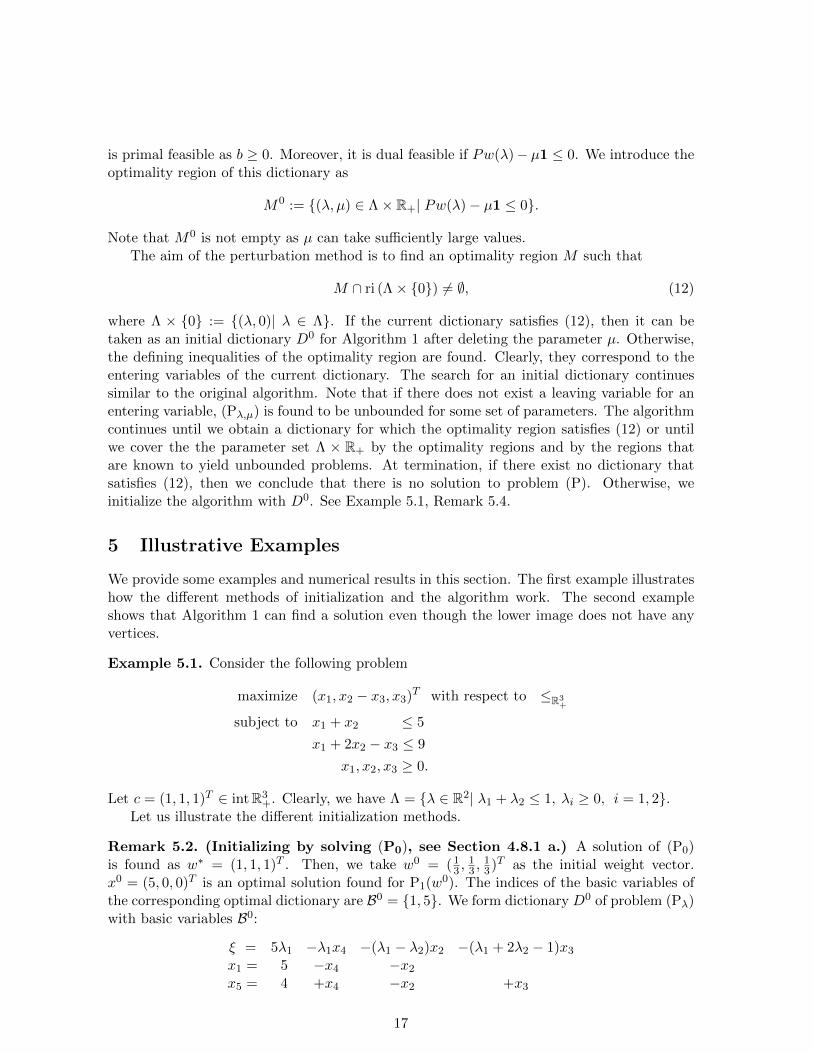
where Λ × {0} := {(λ, 0)| λ ∈ Λ}. If the current dictionary satisfies (12), then it can betaken as an initial dictionary D0 for Algorithm 1 after deleting the parameter µ. Otherwise,the defining inequalities of the optimality region are found. Clearly, they correspond to theentering variables of the current dictionary. The search for an initial dictionary continuessimilar to the original algorithm. Note that if there does not exist a leaving variable for anentering variable, (Pλ,µ) is found to be unbounded for some set of parameters. The algorithmcontinues until we obtain a dictionary for which the optimality region satisfies (12) or untilwe cover the the parameter set Λ × R+ by the optimality regions and by the regions thatare known to yield unbounded problems. At termination, if there exist no dictionary thatsatisfies (12), then we conclude that there is no solution to problem (P). Otherwise, weinitialize the algorithm with D0. See Example 5.1, Remark 5.4.
5 Illustrative Examples
We provide some examples and numerical results in this section. The first example illustrateshow the different methods of initialization and the algorithm work. The second exampleshows that Algorithm 1 can find a solution even though the lower image does not have anyvertices.
Example 5.1. Consider the following problem
maximize (x1, x2 − x3, x3)T with respect to ≤R3+
subject to x1 + x2 ≤ 5
x1 + 2x2 − x3 ≤ 9
x1, x2, x3 ≥ 0.
Let c = (1, 1, 1)T ∈ intR3+. Clearly, we have Λ = {λ ∈ R2| λ1 + λ2 ≤ 1, λi ≥ 0, i = 1, 2}.
Let us illustrate the different initialization methods.
Remark 5.2. (Initializing by solving (P0), see Section 4.8.1 a.) A solution of (P0)is found as w∗ = (1, 1, 1)T . Then, we take w0 = (1
3 ,13 ,
13)T as the initial weight vector.
x0 = (5, 0, 0)T is an optimal solution found for P1(w0). The indices of the basic variables ofthe corresponding optimal dictionary are B0 = {1, 5}. We form dictionary D0 of problem (Pλ)with basic variables B0:
ξ = 5λ1 −λ1x4 −(λ1 − λ2)x2 −(λ1 + 2λ2 − 1)x3
x1 = 5 −x4 −x2
x5 = 4 +x4 −x2 +x3
17

Remark 5.3. (Initializing using the structure of the problem, see Section 4.8.1 b.)The structure of Example 5.1 allows us to initialize without solving a linear program. Considerw0 = (1, 0, 0)T . As the objective of P1(w0) is to maximize x1 and the most restrainingconstraint is x1 +x2 ≤ 5 together with xi ≥ 0, x = (5, 0, 0)T is an optimal solution of P1(w0).The corresponding slack variables are x4 = 0 and x5 = 4. Note that this corresponds tothe dictionary with basic variables {1, 5} and nonbasic variables {2, 3, 4}, which yields thesame initial dictionary D0 as above. Note that one needs to be careful as w0 /∈ intC+ butw0 ∈ bdC+. In order to ensure that the corresponding initial solution is a maximizer and notonly a weak maximizer, one needs to check the optimality region of the initial dictionary. Ifthe optimality region has a nonempty intersection with int Λ, which is the case for D0, thenthe corresponding basic solution is a maximizer. In general, if one can find w ∈ intC+ suchthat (P1(w)) has a trivial optimal solution, then the last step is clearly unnecessary.
Remark 5.4. (Initializing using the perturbation method, see Section 4.8.2.) Thestarting dictionary for (Pλ,µ) of the perturbation method is given as
ξ = −(µ− λ1)x1 −(µ− λ2)x2 −(µ+ λ1 + 2λ2 − 1)x3
x4 = 5 −x1 −x2
x5 = 9 −x1 −2x2 +x3
This dictionary is optimal for M0 = {(λ, µ) ∈ Λ×R| µ−λ1 ≥ 0, µ−λ2 ≥ 0, µ+λ1 +2λ2 ≥ 1}.Clearly, M0 does not satisfy (12). The defining halfspaces for M0 correspond to the nonbasicvariables x1, x2 and x3. If x1 enters, then the leaving variable is x4 and the next dictionary hasthe optimality region M1 = {(λ, µ) ∈ Λ×R| −µ+λ1 ≥ 0, λ1−λ2 ≥ 0, µ+λ1+2λ2 ≥ 1} whichsatisfies (12). Then, by deleting µ the initial dictionary is found to be D0 as above. Differentchoices of entering variables in the first iteration might yield different initial dictionaries.
Consider the initial dictionary D0. Clearly, ID0
4 = {λ ∈ R2| λ1 ≥ 0}, ID0
2 = {λ ∈R2| λ1 − λ2 ≥ 0}, and ID
0
3 = {λ ∈ R2| λ1 + 2λ2 ≥ 1}. The defining halfspaces for ΛD0 ∩ Λ
correspond to the nonbasic variables x2, x3, thus we have JD0
= {2, 3}.The iteration starts with the only boundary dictionary D0. If x2 is the entering variable,
x5 is picked as the leaving variable. The next dictionary, D1, has basic variables B1 = {1, 2},the basic solution x1 = (1, 4, 0)T , and a parameter region ΛD
1= {λ ∈ R2| 2λ1 − λ2 ≥
0, −λ1 + λ2 ≥ 0, 2λ1 + λ2 ≥ 1}. The halfspaces corresponding to the nonbasic variables xj ,
j ∈ JD1= {3, 4, 5} are defining for the optimality region ΛD
1 ∩ Λ. Moreover, ED1
= {(5, 2)}is an explored pivot for D1.
From dictionary D0, for entering variable x3 there is no leaving variable according to theminimum ratio rule (6). We conclude that problem (Pλ) is unbounded for λ ∈ R2 such thatλ1 + 2λ2 < 1. Note that
B−1N =
1 1 0
−1 1 −1
,and the third column corresponds to the entering variable x3. Thus, xhB0 = (xh1 , x
h5)T =
(0,−1)T and xhN 0 = (xh4 , xh2 , x
h3)T = e3 = (0, 0, 1)T . Thus, we add xh = (xh1 , x
h2 , x
h3) =
(0, 0, 1)T to the set X h, see Algorithm 1, line 12. Also, by Proposition 4.3, P Txh = (0,−1, 1)T
is an extreme direction of the lower image P. After the first iteration, we have V S = {D0},and BD = {D1}.
18
For the second iteration, we consider D1 ∈ BD. There are three possible pivots withentering variables xj , j ∈ JD
1= {3, 4, 5}. For x5, x2 is found as the leaving variable. As
(5, 2) ∈ ED1, the pivot is already explored and not necessary. For x3, the leaving variable
is found as x1. The resulting dictionary D2 has basic variables B2 = {2, 3}, basic solutionx2 = (0, 5, 1)T , the optimality region ΛD
2 ∩ Λ = {λ ∈ R2+| 2λ1 + λ2 ≤ 1, 2λ1 + 3λ2 ≤
2, −λ1 − 2λ2 ≤ −1}, and the indices of the entering variables JD2
= {1, 4, 5}. Moreover, wewrite ED
2= {(1, 3)}.
We continue the second iteration by checking the entering variable x4 from D1. Theleaving variable is found as x1. This pivot yields a new dictionary D3 with basic variablesB3 = {2, 4} and basic solution x3 = (0, 4.5, 0)T . The indices of the entering variables arefound as JD
3= {1, 3}. Also, we have ED
3= {(1, 4)}. At the end of the second iteration we
have V S = {D0, D1}, and BD = {D2, D3}.Consider D2 ∈ BD for the third iteration. For x1, the leaving variable is x3 and we
obtain dictionary D1 which is already visited. For x4, the leaving variable is x3. We obtainthe boundary dictionary D3 and update the explored pivots for it as ED
3= {(1, 4), (3, 4)}.
Finally, for entering variable x5 there is no leaving variable and one finds the same xh that isalready found at the first iteration. At the end of third iteration, V S = {D0, D1, D2}, BD ={D3}.
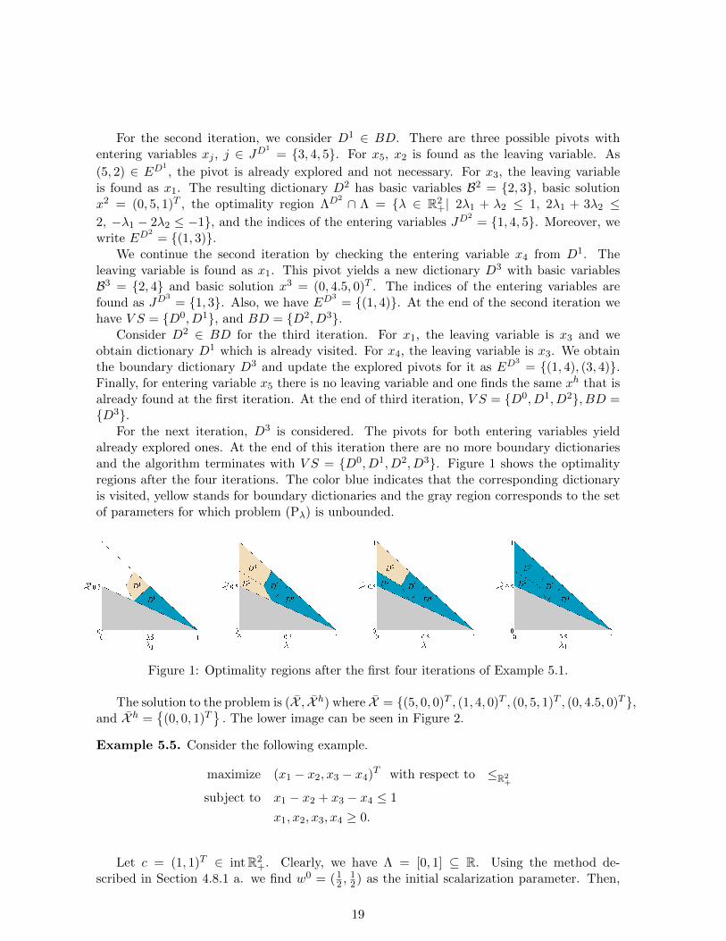
For the next iteration, D3 is considered. The pivots for both entering variables yieldalready explored ones. At the end of this iteration there are no more boundary dictionariesand the algorithm terminates with V S = {D0, D1, D2, D3}. Figure 1 shows the optimalityregions after the four iterations. The color blue indicates that the corresponding dictionaryis visited, yellow stands for boundary dictionaries and the gray region corresponds to the setof parameters for which problem (Pλ) is unbounded.
Figure 1: Optimality regions after the first four iterations of Example 5.1.
The solution to the problem is (X , X h) where X = {(5, 0, 0)T , (1, 4, 0)T , (0, 5, 1)T , (0, 4.5, 0)T },and X h =
{(0, 0, 1)T
}. The lower image can be seen in Figure 2.
Example 5.5. Consider the following example.
maximize (x1 − x2, x3 − x4)T with respect to ≤R2+
subject to x1 − x2 + x3 − x4 ≤ 1
x1, x2, x3, x4 ≥ 0.
Let c = (1, 1)T ∈ intR2+. Clearly, we have Λ = [0, 1] ⊆ R. Using the method de-
scribed in Section 4.8.1 a. we find w0 = (12 ,
12) as the initial scalarization parameter. Then,
19

Figure 2: Lower image P of Example 5.1.
x0 = (1, 0, 0, 0)T is an optimal solution to P1(w0) and the index set of the basic vari-ables of D0 is found as B0 = {1}. Algorithm 1 terminates after two iterations and yieldsX = {(1, 0, 0, 0)T , (0, 0, 1, 0)T }, X h = {(1, 0, 0, 1)T , (0, 1, 1, 0)T }. The lower image can be seenin Figure 3. Note that as it is possible to generate the lower image only with one pointmaximizer, the second one is redundant, see Remark 4.9 b.
0 1 2
0
1
2
x1 − x2
x3−
x4 P
Tx1
PTx0
Figure 3: Lower image P of Example 5.5.
6 Comparison of Different Simplex Algorithms for LVOP
As briefly mentioned in Section 1, there are different simplex algorithms to solve LVOPs.Among them, the Evans-Steuer algorithm [15] works very similar to the algorithm providedhere. It moves from one dictionary to another where each dictionary gives a point maximizer.Moreover, it finds ’unbounded efficient edges’, which correspond to the direction maximizers.Even though the two algorithms work in a similar way, they have some differences thataffect the efficiency of the algorithms significantly. The main difference is that the Evans-Steuer algorithm finds the set of all maximizers whereas Algorithm 1 finds only a subset ofmaximizers, which generates a solution in the sense of Lohne [19] and allows to generate theset of all maximal elements of the image of the feasible set. In general, the Evans-Steueralgorithm visits more dictionaries than Algorithm 1 especially if the problem is degenerate.
First of all, in each iteration of Algorithm 1, for each entering variable xj , only one leavingvariable is picked among the set of all possible leaving variables, see line 12. Differently,the Evans-Steuer algorithm performs pivots xj ↔ xi for all possible leaving variables, i ∈
20

arg mini∈B, (B−1N)ij>0(B−1b)i
(B−1N)ij. If the problem is degenerate, this procedure leads the Evans-
Steuer algorithm to visit much more dictionaries than Algorithm 1 does. In general, theseadditionally visited dictionaries yield maximizers that are already found. In [1, 2], it has beenshown that using the lexicographic rule to choose the leaving variables would be sufficient tocover all the efficient basic solutions. For the numerical tests that we run, see Section 7, wehave modified the Evans-Steuer algorithm such that it uses the lexicographic rule.
Another difference between the two simplex algorithms is at the step where the enteringvariables are selected. In Algorithm 1, the entering variables are the ones which correspondto the defining inequalities of the current optimality region. Different methods to find theentering variables are provided in Section 4.3. The method that is employed for the numericalexamples of Section 7 involves solving sequential LP’s with q− 1 variables and at most n+ kinequality constraints, where k is the number of generating vectors of the ordering cone. Notethat the number of constraints are decreasing in each LP as one solves them successively. Foreach dictionary, the total number of LPs to solve is at most n in each iteration.
The Evans-Steuer algorithm finds a larger set of entering variables, namely ’efficient non-basic variables’ for each dictionary. In order to find this set, it solves n LPs with n + q + 1variables, q equality and n + q + 1 non-negativity constraints. More specifically, for eachnonbasic variable j ∈ N it solves
maximize 1T v
subject to ZTN y − δZTN ej − v = 0,
y, δ, v ≥ 0,
where y ∈ Rn, δ ∈ R, v ∈ Rq. Only if this program has an optimal solution 0, then xj isan efficient nonbasic variable. This procedure is clearly costlier than the one employed inAlgorithm 1. In [17], this idea is improved so that it is possible to complete the procedureby solving fewer LPs of the same structure. Further improvements are done also in [9].Moreover, in [1, 2] a different method is applied in order to find the efficient nonbasic variables.Accordingly, one needs to solve n LPs with 2q variables, n equality and 2q nonnegativityconstraints. Clearly, this method is more efficient than the one used for the Evans-Steueralgorithm. However, the general idea of finding the efficient nonbasic variables clearly yieldsvisiting more redundant dictionaries than Algorithm 1 would visit. Some of these additionallyvisited dictionaries yield different maximizers that map into already found maximal elementsin the objective space, see Example 6.1; while some of them yield non-vertex maximal elementsin the objective space, see Example 6.2.
Example 6.1. Consider the following simple example taken from [27], in which it has beenused to illustrate the Evans-Steuer algorithm.
maximize (3x1 + x2, 3x1 − x2)T with respect to ≤R2+
subject to x1 + x2 ≤ 4
x1 − x2 ≤ 4
x3 ≤ 4
x1, x2, x3 ≥ 0.
If one uses Algorithm 1, the solution is provided right after the initialization. The initialset of basic variables can be found as B0 = {1, 5, 6}, and the basic solution corresponding
21

to the initial dictionary is x0 = (4, 0, 0)T . One can easily check that x0 is optimal for allλ ∈ Λ. Thus, Algorithm 1 stops and returns the single maximizer. On the other hand, it isshown in [27] that the Evans-Steuer algorithm terminates only after performing another pivotto obtain a new maximizer x1 = (4, 0, 4)T . This is because, from the dictionary with basicvariables B0 = {1, 5, 6} it finds x3 as an efficient nonbasic variable and performs one morepivot with entering variable x3. Clearly the image of x1 is again the same vertex (4, 4)T inthe image space. Thus, in order to generate a solution in the sense of Definition 3.1, the lastiteration is unnecessary.
Example 6.2. Consider the following example.
maximize (−x1 − x3,−x2 − 2x3)T with respect to ≤R2+
subject to − x1 − x2 − 3x3 ≤ −1
x1, x2, x3 ≥ 0.
First, we solve the example by Algorithm 1. Clearly, Λ = [0, 1] ⊆ R. We find an initialdictionary D0 with B0 = {1}, which yields the maximizer x0 = (1, 0, 0)T . One can easilysee that index set of the defining inequalities of the optimality region can be chosen eitheras JD
0= {2} or JD
0= {3}. Note that Algorithm 1 picks one of them and continues with
it. In this example we get JD0
= {2}, perform the pivot x2 ↔ x1 to get D1 with B1 = {2}and x1 = (0, 1, 0)T . From D1, there are two choices of sets of entering variables and weset JD
1= {1}. As the pivot x1 ↔ x2 is already explored, the algorithm terminates with
X = {x0, x1} and X h = ∅.When one solves the same problem by the Evans-Steuer algorithm, from D0, both x2 and
x3 are found as entering variables. When x3 enters from D0, one finds a new maximizerx2 = (0, 0, 1
3)T . Note that this yields a nonvertex maximal element on the lower image, seeFigure 4.
−2 −1 0−2
−1
0
−x1 − x3
−x2−
2x3
PTx0
PTx2
PTx1
Figure 4: Lower image P of Example 6.2.
Remark 6.3. Note that if the problem is primal nondegenerate, then for a given enteringvariable of a given dictionary, both Algorithm 1 and the Evans-Steuer algorithm find theunique leaving variable. If in addition, every efficient nonbasic variable of a given dictionarycorresponds to a defining inequality of its optimality region, then the entering variables fromthat dictionary would be the same for both algorithms. Indeed, the different type of redun-dancies that are explained in Remark 4.9 are mostly observed if there is a primal degeneracyor if there are efficient nonbasic variables which corresponds to redundant inequalities of theoptimality region. Hence, it wouldn’t be wrong to state that for ’nondegenerate’ problems,Evans-Steuer algorithm and Algorithm 1 follow similar paths. But for degenerate problemstheir performance will be quite different.
22
Apart from the Evans-Steuer algorithm Ehrgott, Puerta and Rodriguez-Chıa [13] devel-oped a primal-dual simplex algorithm to solve LVOPs. The algorithm finds a partition (Λd)of Λ. It is similar to Algorithm 1 in the sense that for each parameter set Λd, it provides anoptimal solution xd to the problems (Pλ) for all λ ∈ Λd. The difference between the two algo-rithms is in the method of finding the partition. The algorithm in [13] starts with a (coarse)partition of the set Λ. In each iteration it finds a finer partition until no more improvementscan be done. In contrast to the algorithm proposed here, the algorithm in [13] requires solvingin each iteration an LP with n+m variables and l constraints where m < l ≤ m+ n, whichclearly makes the algorithm computationally much more costly. In addition to solving one’large’ LP, it involves a procedure which is similar to finding the defining inequalities of aregion given by a set of inequalities. Also, different from Algorithm 1, it finds only a set ofweak maximizers so that as a last step one needs to perform a vertex enumeration in orderto obtain a solution consisting of maximizers only. Finally, the algorithm provided in [13]can deal with unbounded problems only if the set Λb is provided, which requires a Phase 1procedure.
7 Numerical Results
In this section we provide numerical results to study the efficiency of Algorithm 1. Wegenerate random problems, solve them with different algorithms and compare the solutionsand the CPU times. Algorithm 1 is implemented in MATLAB. We also use a MATLABimplementation of Benson’s algorithm, namely bensolve 1.2 [20]. The current version ofbensolve 1.2 solves two linear programs in each iteration. However, we employ an improvedversion which solves only one linear program in each iteration, see [16]. For the Evans-Steueralgorithm, instead of using ADBASE [30], we implement the algorithm in MATLAB. Thisway, we could test the algorithms with the same machinery. This gives the opportunity tocompare the CPU times. For each algorithm the linear programs are solved using the GLPKsolver, see [25].
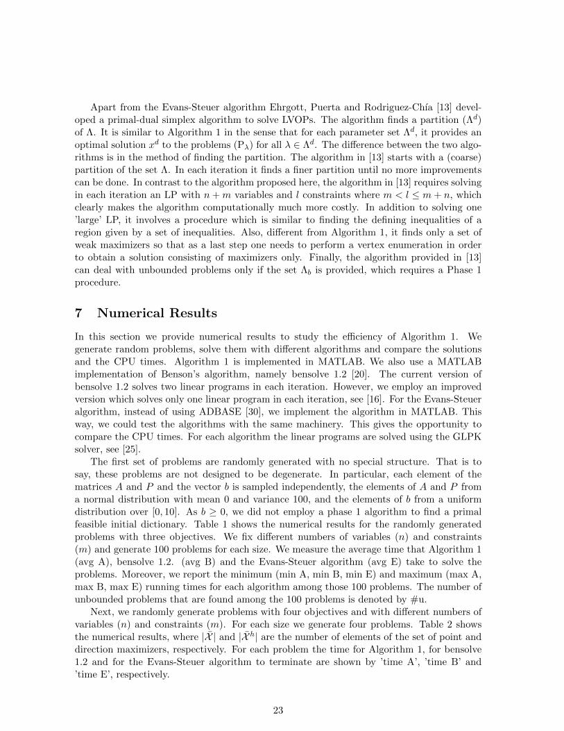
The first set of problems are randomly generated with no special structure. That is tosay, these problems are not designed to be degenerate. In particular, each element of thematrices A and P and the vector b is sampled independently, the elements of A and P froma normal distribution with mean 0 and variance 100, and the elements of b from a uniformdistribution over [0, 10]. As b ≥ 0, we did not employ a phase 1 algorithm to find a primalfeasible initial dictionary. Table 1 shows the numerical results for the randomly generatedproblems with three objectives. We fix different numbers of variables (n) and constraints(m) and generate 100 problems for each size. We measure the average time that Algorithm 1(avg A), bensolve 1.2. (avg B) and the Evans-Steuer algorithm (avg E) take to solve theproblems. Moreover, we report the minimum (min A, min B, min E) and maximum (max A,max B, max E) running times for each algorithm among those 100 problems. The number ofunbounded problems that are found among the 100 problems is denoted by #u.
Next, we randomly generate problems with four objectives and with different numbers ofvariables (n) and constraints (m). For each size we generate four problems. Table 2 showsthe numerical results, where |X | and |X h| are the number of elements of the set of point anddirection maximizers, respectively. For each problem the time for Algorithm 1, for bensolve1.2 and for the Evans-Steuer algorithm to terminate are shown by ’time A’, ’time B’ and’time E’, respectively.
23
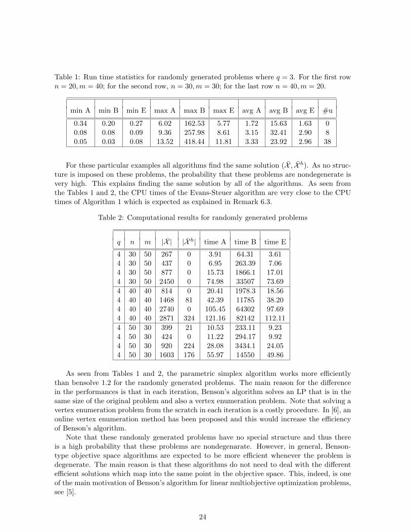
Table 1: Run time statistics for randomly generated problems where q = 3. For the first rown = 20,m = 40; for the second row, n = 30,m = 30; for the last row n = 40,m = 20.
min A min B min E max A max B max E avg A avg B avg E #u
0.34 0.20 0.27 6.02 162.53 5.77 1.72 15.63 1.63 00.08 0.08 0.09 9.36 257.98 8.61 3.15 32.41 2.90 80.05 0.03 0.08 13.52 418.44 11.81 3.33 23.92 2.96 38
For these particular examples all algorithms find the same solution (X , X h). As no struc-ture is imposed on these problems, the probability that these problems are nondegenerate isvery high. This explains finding the same solution by all of the algorithms. As seen fromthe Tables 1 and 2, the CPU times of the Evans-Steuer algorithm are very close to the CPUtimes of Algorithm 1 which is expected as explained in Remark 6.3.
Table 2: Computational results for randomly generated problems
q n m |X | |X h| time A time B time E
4 30 50 267 0 3.91 64.31 3.614 30 50 437 0 6.95 263.39 7.064 30 50 877 0 15.73 1866.1 17.014 30 50 2450 0 74.98 33507 73.69
4 40 40 814 0 20.41 1978.3 18.564 40 40 1468 81 42.39 11785 38.204 40 40 2740 0 105.45 64302 97.694 40 40 2871 324 121.16 82142 112.11
4 50 30 399 21 10.53 233.11 9.234 50 30 424 0 11.22 294.17 9.924 50 30 920 224 28.08 3434.1 24.054 50 30 1603 176 55.97 14550 49.86
As seen from Tables 1 and 2, the parametric simplex algorithm works more efficientlythan bensolve 1.2 for the randomly generated problems. The main reason for the differencein the performances is that in each iteration, Benson’s algorithm solves an LP that is in thesame size of the original problem and also a vertex enumeration problem. Note that solving avertex enumeration problem from the scratch in each iteration is a costly procedure. In [6], anonline vertex enumeration method has been proposed and this would increase the efficiencyof Benson’s algorithm.
Note that these randomly generated problems have no special structure and thus thereis a high probability that these problems are nondegenarate. However, in general, Benson-type objective space algorithms are expected to be more efficient whenever the problem isdegenerate. The main reason is that these algorithms do not need to deal with the differentefficient solutions which map into the same point in the objective space. This, indeed, is oneof the main motivation of Benson’s algorithm for linear multiobjective optimization problems,see [5].
24

In order to see the efficiency of our algorithm for degenerate problems, we generate randomproblems which are designed to be degenerate. In the following examples this is done by gen-erating a nonnegative b vector with many zero components and choosing objective functionswith the potential to create optimality regions with empty interior within Λ. In particular,for the three-objective examples, we generate the first objective function randomly, take thesecond one to be the negative of the first objective function, and let the third objective con-sist of only one nonzero entry. For the four-objective examples, the first three objectives arecreated as described above and the fourth one is generated randomly in a way that at leasthalf of its components are zero.
First, we consider three objective functions where we fix different numbers of variables (n)and constraints (m). We generate 20 problems for each size. We measure the average timethat Algorithm 1 (avg A), bensolve 1.2. (avg B) and the Evans-Steuer algorithm (avg E) taketo solve the problems. We also report the minimum (min A, min B, min E) and maximum(max A, max B, max E) running times for each algorithm among those 20 problems. Thetimes are measured in seconds. The results are given in Table 3.
Table 3: Run time statistics for randomly generated degenerate problems where q = 3. For thefirst row n = 5,m = 15; for the second row n = m = 10; and for the last row n = 15,m = 5.
min A min B min E max A max B max E avg A avg B avg E
0.02 0.01 0.03 0.14 0.09 140.69 0.07 0.04 8.850.03 0.02 0.08 1.33 0.14 4194.1 0.25 0.04 227.020.05 0.01 0.09 1.47 0.20 1893.0 0.05 0.25 190.25
In order to give an idea how the solutions provided by the three algorithms differ for thesedegenerate problems, in Table 4 we provide detailed results for single problems. Among the20 problems that are generated to obtain each row of Table 3, we select the two problemswith the CPU times ’max A’ and ’max E’ and provide the following for them. |X(·)| and
|X h(·)| denote the number of elements of the set of point and direction maximizers that are
found by each algorithm, respectively. |V SA| and |V SE | are the number of dictionaries thatAlgorithm 1 and the Evans-Steuer algorithm visit until termination. For each problem thetime for Algorithm 1, bensolve 1.2, and the Evans Steuer algorithm to terminate are shownby ’time A’, ’time B’ and ’time E’, respectively.
Finally, we compare Algorithm 1 and bensolve 1.2 to get statistical results regarding theirefficiencies for degenerate problems. Note that this test was done on a different computerthan the previous tests. Table 5 shows the numerical results for the randomly generateddegenerate problems with q = 4 objectives, m constraints and n variables. We generate 100problems for each size. We measure the average time that Algorithm 1 (avg A) and bensolve1.2. (avg B) take to solve the problems. The minimum (min A, min B) and maximum (maxA, max B) running times for each algorithm among those 100 problems are also provided.
Clearly, for degenerate problems bensolve 1.2 is more efficient than the simplex-type al-gorithms considered here, namely Algorithm 1 and the Evans-Steuer algorithm. However,the design of Algorithm 1 results in a significant decrease in CPU time compared to theEvans-Steuer algorithm in its improved form of [1, 2].
25

Table 4: Computational results for single problems that require CPU times max A and maxE among the ones that are generated for Table 3. For the first set of problems n = 5,m = 15;for the second set of problems n = m = 10 (max A and max E yielded the same problemhere); and for the last set of problems n = 15,m = 5.
|V SA| |V SE | |XA| |XB| |XE | |X hA| |X hB| |X hE | time A time B time E
20 5617 1 1 1 0 0 0 0.13 0.03 140.6930 361 3 3 3 0 0 0 0.14 0.06 6.61
324 22871 1 1 4 0 0 1 1.33 0.03 4194.1
14 11625 1 1 1 0 0 0 0.05 0.03 1893.0452 11550 1 1 1 39 2 4707 1.47 0.05 1598.1
Table 5: Run time statistics for randomly generated degenerate problems.
q n m min A min B max A max B avg A avg B
4 10 30 0.05 0.03 177.47 4.07 8.49 0.214 20 20 0.21 0.02 973.53 199.77 19.89 12.054 30 10 0.11 0.03 2710.20 13.70 37.68 0.73
Acknowledgements
We would like to thank Andreas Lohne, Friedrich-Schiller-Universitat Jena, for helpful re-marks that greatly improved the manuscript, and Ralph E. Steuer, University of Georgia, forproviding us the ADBASE implementation of the algorithm from [15].
References
[1] Armand, P.: Finding all maximal efficient faces in multiobjective linear programming.Mathematical Programming 61, 357–375 (1993)
[2] Armand, P., Malivert, C.: Determination of the efficient set in multiobjective linearprogramming. Journal of Optimization Theory and Applications 70, 467–489 (1991)
[3] Barber, C.B., Dobkin, D.P., Huhdanpaa, H.T.: The Quickhull algorithm for convex hulls.ACM Transactions on Mathematical Software 22(4), 469–483 (1996)
[4] Bencomo, M., Gutierrez, L., Ceberio, M.: Modified Fourier-Motzkin elimination algo-rithm for reducing systems of linear inequalities with unconstrained parameters. Depart-mental Technical Reports (CS) 593, University of Texas at El Paso (2011)
[5] Benson, H.P.: An outer approximation algorithm for generating all efficient extremepoints in the outcome set of a multiple objective linear programming problem. Journalof Global Optimization 13, 1–24 (1998)
[6] Csirmaz, L.: Using multiobjective optimization to map the entropy region. Computa-tional Optimization and Applications 63(1), 45–67 (2016)
26

[7] Dauer, J.P.: Analysis of the objective space in multiple objective linear programming.Journal of Mathematical Analysis and Applications 126(2), 579–593 (1987)
[8] Dauer, J.P., Liu, Y.H.: Solving multiple objective linear programs in objective space.European Journal of Operational Research 46(3), 350–357 (1990)
[9] Ecker, J.G., Hegner, N.S., Kouada, I.A.: Generating all maximal efficient faces for mul-tiple objective linear programs. Journal of Optimization Theory and Applications 30,353–381. (1980)
[10] Ecker, J.G., Kouada, I.A.: Finding all efficient extreme points for multiple objectivelinear programs. Mathematical Programming 14(12), 249–261 (1978)
[11] Ehrgott, M.: Multicriteria Optimization. Springer-Verlag, Berlin, Heidelberg (2005)
[12] Ehrgott, M., Lohne, A., Shao, L.: A dual variant of Benson’s outer approximationalgorithm. Journal Global Optimization 52(4), 757–778 (2012)
[13] Ehrgott, M., Puerto, J., Rodriguez-Chıa, A.M.: Primal-dual simplex method for multi-objective linear programming. Journal of Optimization Theory and Applications 134,483–497 (2007)
[14] Ehrgott, M., Shao, L., Schobel, A.: An approximation algorithm for convex multi-objective programming problems. Journal of Global Optimization 50(3), 397–416 (2011)
[15] Evans, J.P., Steuer, R.E.: A revised simplex method for multiple objective programs.Mathematical Programming 5(1), 54–72 (1973)
[16] Hamel, A.H., Lohne, A., Rudloff, B.: Benson type algorithms for linear vector optimiza-tion and applications. Journal of Global Optimization 59(4), 811–836 (2014)
[17] Isermann, H.: The enumeration of the set of all efficient solutions for a linear multipleobjective program. Operational Research Quarterly 28(3), 711–725 (1977)
[18] Kalyanasundaram, B., Pruhs, K.R.: Constructing competetive tours from local informa-tion. Theoretical Computer Science 130, 125–138 (1994)
[19] Lohne, A.: Vector Optimization with Infimum and Supremum. Springer (2011)
[20] Lohne, A.: BENSOLVE: A free VLP solver, version 1.2. (2012). URLhttp://ito.mathematik.uni-halle.de/ loehne
[21] Lohne, A., Rudloff, B., Ulus, F.: Primal and dual approximation algorithms for convexvector optimization problems. Journal of Global Optimization 60(4), 713–736 (2014)
[22] Lohne, A., Weißing, B.: BENSOLVE: A free VLP solver, version 2.0.1 (2015). URLhttp://bensolve.org/
[23] Lohne, A., Weißing, B.: The vector linear program solver bensolve – notes ontheoretical background. European Journal of Operational Research (2016). DOI10.1016/j.ejor.2016.02.039
27

[24] Luc, D.: Theory of Vector Optimization, Lecture Notes in Economics and MathematicalSystems, vol. 319. Springer Verlag, Berlin, Heidelberg (1989)
[25] Makhorin, A.: GLPK (GNU linear programming kit) (2012). URLhttps://www.gnu.org/software/glpk/
[26] Ruszczynski, A., Vanderbei, R.J.: Frontiers of stochastically nondominated portfolios.Econometrica 71(4), 1287–1297 (2003)
[27] Schechter, M., Steuer, R.E.: A correction to the connectedness of the evans-steuer algo-rithm of multiple objective linear programming. Foundations of Computing and DecisionSciences 30(4), 351–359 (2005)
[28] Shao, L., Ehrgott, M.: Approximately solving multiobjective linear programmes in ob-jective space and an application in radiotherapy treatment planning. MathematicalMethods of Operations Research 68(2), 257–276 (2008)
[29] Shao, L., Ehrgott, M.: Approximating the nondominated set of an MOLP by approxi-mately solving its dual problem. Mathematical Methods of Operations Research 68(3),469–492 (2008)
[30] Steuer, R.E.: A multiple objective linear programming solver for all efficient extremepoints and all unbounded efficient edges. Terry College of Business, University of Georgia,Athens, Georgia (2004)
[31] Vanderbei, R.J.: Linear Programming: Foundations and Extensions. Kluwer AcademicPublishers (2013)
[32] Zionts, S., Wallenius, J.: Identifying efficient vectors: some theory and computationalresults. Operations Research 28(3), 786–793 (1980)
28