on gradient simplex methods for linear programs · on gradient simplex methods for linear ......

JOURNAL OF APPLIED MATHEMATICS AND DECISION SCIENCES, 8(2), 107–129Copyright c© 2004, Lawrence Erlbaum Associates, Inc.

On Gradient Simplex Methods for LinearPrograms

R. R. VEMUGANTI† [email protected]

Merrick School of Business, University of Baltimore, MD 21201, USA

Abstract. A variety of pivot column selection rules based upon the gradient criteria(including the steepest edge) have been explored to improve the efficiency of the primalsimplex method. Simplex-like algorithms have been proposed imbedding the gradientdirection (GD) which includes all variables whose increase or decrease leads to an im-provement in the objective function. Recently a frame work has been developed in thesimplex method to incorporate the reduced-gradient direction (RGD) consisting of onlyvariables whose increase leads to an improvement in the objective function. In this pa-per, the results are extended to embed GD in the simplex method based on the conceptof combining directions. Also mathematical properties related to combining directionsas well as deleting a variable from all basic directions are presented.

Keywords: Gradient Directions, Linear Programming, Simplex Algorithm.

1. Introduction

Consider the linear program (LP(1)):

Max z = ctx (1)s.t. Ax = b and x ≥ 0

where ct = (c1, . . . , cn), bt = (b1, . . . , bm) , xt = (x1, . . . , xn) and A =(aij) is a m × n matrix. Suppose B is the basis matrix corresponding toa feasible extreme point and let aj be the column corresponding to thevariable xj . Also let xB and xN be the set of basic and nonbasic variablescorresponding to the basis matrix B. Partitioning the matrix A and thevector ct corresponding to the basic and nonbasic variables into A = (B,N) and ct = (ct

B , ctN ), the linear programming in (1) can be written as

Max z = ctBB−1b + ct

NxN (2)s.t. xB + B−1NxN = B−1b = b and (xB , xN ) ≥ 0

where ctN = (ct

N − ctBB−1N). Clearly the solution is optimal if cN ≤ 0.

When one or more cj , j ∈ xN are positive the objective function value may

† Requests for reprints should be sent to R. R. Vemuganti, Merrick School of Business,University of Baltimore, 1420 North Charles Street, Baltimore, MD 21201, USA.

108 R. R. VEMUGANTI

be improved by replacing one of the basic variables (pivot row) with one ofthe nonbasic variables xj (pivot column) for which cj > 0. In the steepestunit ascent method (Dantzig(63)), the variable with the largest positive cj

is selected to enter the basis. To maintain primal feasibility the departingvariable xp is chosen using the rule

bp/apk = mini(bi/aik, aik > 0)

where k is the entering variable and aj = (aij) is the column correspondingto xj in the formulation (2). If no such departing variable exists, theproblem is unbounded. When there is a tie, Bland’s (77) rule may be usedto avoid cycling. An improvement over the unit ascent rule is to select thevariable k for which the change in the objective function given by ck(bp/apk)is a maximum.Computationally more expensive gradient criteria for the selection of thepivot column can be found in Abel (87), Goldfarb and Reid (77), Harris(73), and Zoutenddijk (76). For example if the Np -norm of (aj , h) is givenby

Np(aj , h) = [m∑

i=1

(|aij |+ |h|)p]1/p

for1 ≤ p < ∞

N∞(aj , h) = Max(|ai1|, . . . , |ain|, |h|)

then the gradient of the variable j is gpj = cj/Np(aj , h). Including only

the positive values or negative values or both of aj in the Np− norm andsetting h = 1 or cj , a variety of gradients can be generated. Under thegradient criteria, the variable with the largest gradient value for whichcj > 0 is selected. The gradient g2

j when h=1 corresponds to the steepestedge. Abel (87) reports the gradient criterion for p=1 and h=1, appearsto perform better requiring fewer iterations when compared with severalother gradients by changing the values of p. Computational experimentsby Goldfarb and Reid (77) indicate that the steepest edge criterion is moreefficient than the rule of selecting the variable with the most positive cj .Attempts to bring more than one variable into the basis simultaneouslyare limited to two variables (Paranjape (65) ) due to excessive computa-tional effort. Another approach called gradient method, which attemptsto combine all eligible variables into a bundle is addressed by Beilby (76),Eislet and Sandblom (90), Fathi and Murty (89), Graves and Wolfe (64),Heady and Candler (58), Kallio and Porteus (78), Mitra, Tamiz and Yade-gar (88). Following the development of Kallio and Porteus (78), supposex is a feasible solution corresponding to a basis where some nonbasic vari-ables are permitted to be at a positive level. For each nonbasic variable j,

ON GRADIENT SIMPLEX METHODS FOR LPS 109

let dj = (dij), be an n dimensional vector given by

dij =

aij if i is a basic variable1 if i = j0 otherwise.

Determine the direction d by combining the columns dj , with weights givenby

wj ={

cj if cj < 0 and xj > 0 or cj > 00 otherwise.

Now consider the new solution x = x + αd where d =∑n

j=1 wjdj . Findthe largest step size α∗ for which x ≥ 0. Clearly the new solution is givenby x = x + α∗d and the increase in the objective function is α∗

∑nj=1 c2

j .When a nonbasic variable decreases to zero in the solution, the procedureis continued. When one or more basic variables are driven to zero, oneof these basic variables is replaced by the first candidate in the list of thenonbasic variables. The departing variable is added to the list of the non-basic variables. Fathi and Murty (89) and Mitra, Tamiz and Yadegar (88),provide a mechanism to construct a basic feasible solution from x with theobjective function value ≥ ctx before generating the next direction. Thismethod is proven to converge (Kallio and Porteus (78)) in a finite num-ber of iterations when the LP is non degenerate. As noted by Graves andWolfe (64), this approach is similar to the gradient methods (Rosen (61)and Kreko (68)), in using the gradient to determine the desired directionof movement and is not conveniently illustrated geometrically.Eislet and Sandblom (90) and Zipkin (80), developed a framework to embedreduced-gradient direction (RGD) called external pivoting in the simplexmethod where the variables in the gradient direction are restricted only tothose nonbasic variables for which cj > 0. In this paper the results are ex-tended to develop a frame work to incorporate the gradient direction (GD)in the simplex method and two algorithms are presented to implement thescheme. The next section deals with the frame work to embed RGD andGD in the simplex method.

2. Gradient Simplex Method Framework

Suppose Qk is a subset of variables v = (1,2,....,n). Define a variable yk

with a column vector dk and the coefficient in the objective function fk

110 R. R. VEMUGANTI

given by

dk =∑

j∈Qk

wjkaj and fk =∑

j∈Qk

wjkcj (3)

where |wjk| > 0 for j ∈ Qk and wjk = 0 otherwise and∑

j∈Qk|wjk| = 1.

Excluding the singleton sets and the empty set, noting the fact that eachweight wjk can be positive or zero or negative, the number of y-variablesone can construct is r = 3n − (n + 1). Now consider the LP (3) with nx-variables and r y-variables given by

Max z = ctx + f ty (4)s.t. Ax + Dy = b, Ix + Wy ≥ 0 and x ≥ 0, y ≥ 0

where D = (d1, . . . , dr) is a m× r matrix, W = (wjk) is a n× r matrix, Iis a n × n identity matrix and yt = (y1, . . . , yr). It is easy to verify thatif x∗ is a feasible solution to LP(1) then x = x∗ and y = 0 is a feasiblesolution to LP(3). Conversely if (x∗, y∗) is a feasible solution to LP(3)then x = x∗+Wy∗ is a feasible solution to LP(1). Since the correspondingobjective functions are equal it is clear that an optimal solution to LP(1)can be found by solving LP(3).

When the weights wij are restricted to be nonnegative (RGD), the num-ber of y-variables that can be formed is reduced to r = 2n − (n + 1) andthe second set of constraints in formulation 4 is redundant. As described inEislet and Sandblom (90) and Zipkin(80), to embed the RGD in the sim-plex method, let aij , bi and cj be the elements of any tableau. Constructthe variable yk with weights

wjk ={

cj/γ if j ∈ Qk = (j |cj > 0)0 otherwise

where γ =∑

j∈Qkcj . Determine the corresponding column vector dk and

the objective function coefficient fk from (3). Pivot the variable yk into thebasis and continue the procedure till an optimal solution is found. In thenext section the results are extended to embed GD in the simplex methodbased on the concept of combining directions and related mathematicalproperties.

3. Gradient Simplex Method

It appears that the formulation (4) requires a basis size of (m+n) to imple-ment the simplex method. The following analysis and results are directed


towards developing a technique to embed GD in the simplex method witha basis of size m. Suppose the weights for a singleton basic variable xk

are given by wjk = cj / |cj | = ± 1 (|cj | > 0) if j = k and zero, otherwise.Now consider any basis of formulation LP(3) with weights for the m basicvariables (k(1),. . ., k(m)) given by wjk(i) , for i = (1,..., m) and j = (1,...,n). It is clear that the values of the variables xj , for j = (1,2 ..., n), in theformulation LP(1) can be obtained from

xj =m∑

i=1

wjk(i)bi. (5)

Assuming that the selected set of basic directions and the correspondingstep lengths yielded all xj ≥ 0 in (5) at some iteration (t-1), consider anew direction wjt = wjt/γ at iteration t where

wjt ={

cj if cj > 0 or cj < 0 and xj > 00 otherwise (6)

where γ =∑n

j=1 |wjt|. If there is no such direction clearly the currenttableau is optimal. If the step length of the new direction is α, then thenew solution xj is given by

xj =∑m

i=1 wjk(i)(bi − αdit) + αwjt (7)

=∑m

i=1 wjk(i)bi + α(wjt −∑m

i=1 wjk(i)dit)= xj + αθjt

where dit =∑n

j=1 aijwjt and ft =∑n

j=1 cjwjt. If all θjt ≥ 0, the objectivefunction can be made as large as possible by selecting large values for α andhence the problem is unbounded. If for some j, θjt < 0, then the maximumstep length α∗t to maintain primal feasibility is given by

α∗t = minj(−xj/θjt, θjt < 0) = −xr/θrt. (8)

Having determined the step length α∗t , the following analysis provides amechanism to pivot a new direction into the basis. Suppose for each vari-able j, P (j) = (i, wjk(i) 6= 0) and NP(j) represents the number of elements inP(j). It is easy to verify from (7), moving along the generated direction bythe step length in (8) reduces the value of xr to zero. There are three cases.

CASE 1: xr is basic and NP(r) =1Since xr is a basic variable and NP(r) = 1, cr = wrt = 0, wrk(i) = 0 when

112 R. R. VEMUGANTI

i 6= r and wrk(r) = 1. Therefore from (7), it follows that θrt = −drt whichimplies bk(r) / drt = −xr / θrt = α∗t and hence the basic variable xr can bereplaced by the new direction. If any of the updated bi are negative, thenchange it to −bi and multiply the corresponding weights of the directionby -1.

CASE 2: α∗t > 0 and xr is nonbasic or NP(r) ≥ 2In this case it is possible to generate more than one direction. Suppose forv = 1, wv

t = (wvjt), dv

t = (dvit), fv

t > 0 and α∗tv are the normalized weights,the elements of the column vector, the coefficient in the objective functionand the step length of the first direction. Also let x

(v−1)j be the values of

the variables prior to generating the direction number v. After generatingthe direction number v, update the values of the variables xj to xv

j =

x(v−1)j + α∗tvwv

jt. Using these updated values of xj and the relationship(6), determine the weights of the new direction. If such a direction doesnot exist or the corresponding α∗tv = 0, or it has been generated before(to prevent zigzagging), stop generating additional directions. Suppose his the number of directions generated and let

wjt =∑h

v=1(α∗tvwv

jt), dit =h∑

v=1

(α∗tvdvit) (9)

f t =∑h

v=1(α∗tvfv

t ), λ =n∑

j=1

|wjt|.

The following results are useful in combining these h directions into a singledirection.

Lemma 1 λ > 0.

Proof: From (9), λ = 0 implies |wjt| = wjt =∑h

v=1 α∗tvwvjt = 0 for all

j. After generating the h directions the values of the variables xj = xhj are

given by

xhj = x0

j +h∑

v=1

α∗tvwvjt = x0

j + wjt = x0j . (10)

From (10) it follows that the increase in the objective function is zero whichis a contradiction since the increase in the objective function is f t > 0.

Theorem 1 After normalization, let wjt = (wjt/λ), dit = dit/λ and ft =f t/λ. Then the step length of the combined direction is λ.


Proof: First note that cj values remain the same for all the h directionsgenerated as well as for the combined direction. Also moving a step lengthof α∗tv along each direction for v = (1,...,h) and the maximum step lengthα∗t along the combined single direction results in the same increase in theobjective function. It is clear that the increase in the objective functionmoving along the combined direction is given by α∗t ft = α∗t

∑nj=1 cjwjt.

Substituting for wjt from (9), it is easy to verify that α∗t = λ.Having combined all h directions to a single direction, let xr be a variable

driven to zero. If it is a basic variable and NP(r) = 1, replace this variablewith the direction generated as in the Case 1. Otherwise generate anentering direction by combining the new direction with all basic directionsin P(r). Moving a step length of λ along the generated single directionreduces the step lengths of the basic directions (RHS of the simplex tableau)to (bi - λdit). Using these step lengths as weights, the weights of theentering direction are

wj =∑

v∈P (r)

(bv − λdvt)wjk(v) + λwjt. (11)

Lemma 2 Suppose γ =∑n

j=1 |wj |. Then γ = 0 implies bi = 0 for alli ∈ P (r), dit = 0 for all i /∈ P (r) and ft = 0.

Proof: Clearly γ = 0 implies |wj | = wj = 0 which in turn follows from(11)

λwjt =∑

v∈P (r)

wjk(v)(λdvt − bv). (12)

Multiplying both sides of the equation (12) by aij and summing from j=1to n results in (after rearranging the terms)

λn∑

j=1

wjtaij = λdit =∑

v∈P (r)

(λdvt − bv)dik(v)

where dik(v) are the elements of the column vector of the basic variablek(v) which is an identity column. Therefore it follows λdit = (λdit− bi) fori ∈ P (r) and λdit = 0 for i /∈ P (r). To prove the second part multiplyingboth sides of the equation (12) by cj and summing over j = 1 to n resultsin

λn∑

j=1

wjtcj =∑

v∈P (r)

(λdvt − bv)fk(v) = λft.

114 R. R. VEMUGANTI

Since k(v) for v ∈ P (r) are basic variables, fk(v) = 0 and therefore ft = 0.

Corollary 1. When λ > 0 and ft > 0 then γ > 0.

Theorem 2 Suppose λ > 0 and ft > 0 . When the weights of the enteringdirection from(11) are normalized, let wj = wj/γ. Then the column vectord = (di) of the entering direction is given by di = bi/γ for i ∈ P (r) andλdit/γ for i /∈ P (r).

Proof: By definition the elements of the vector d are given by di =∑nj=1(aijwj/γ). Substituting for wj from (11) and simplifying yields ( see

lemma 2 )

di = (1/γ)∑

v∈P (r)

(bv − λdvt)dik(v) + (λ/γ)dit

where dik(v) are the elements of the column vector of a basic variable inthe current tableau which is an identity column. Therefore dik(v) = 1 if i =v and zero, otherwise. Substituting for dik(v) in the above expression therequired result follows.

Theorem 3 The step length of the entering direction with weights wj =wj/γ as in (11) is γ. In addition, the step lengths of the combined directionand the entering direction yield the same increase in the objective function.

Proof: To determine the step length of the entering direction, let θj andθjt be the values of θ corresponding to the entering and combined directionsrespectively. Then from(7), θj = (wj/γ −

∑mi=1 wjk(i)di). Substituting for

wj from (11) and for di from Theorem(2) results in

θj = (1/γ)∑

v∈P (r)

(bv − λdvt)wjk(v) + (λ/γ)wjt

−∑

v∈P (r)

wjk(v)(bv/γ)−∑

v/∈P (r)

wjk(v)(λ/γ)dit

= (λ/γ)[wjt −m∑

i=1

wjk(i)dit] = (λ/γ)θjt.

Since λ is the maximum step length possible along the combined directionand the variable xr is driven to zero at the maximum step length, it followsfrom (8)

λ = minj(−xj/θjt, θjt < 0) = −xr/θrt.

Since θj = (λ/γ)θjt for all j = (1, . . . , n), the variable xr is also forced tozero at the maximum step along the entering direction and therefore the


maximum step length is given by −xr/θr = (−xr/θjt)(γ/λ) = γ.Substituting for wj from (11) it is straight forward to show that f, thecoefficient of entering direction in the objective function is given by

f =n∑

j=1

cjwj = 1/γ)n∑

j=1

cjwj = (λ/γ)ft.

This proves the second part of the result γf = λft.

Lemma 3 The entering direction can be pivoted into the basis by replacingany of the basic directions v ∈ P (r) for which bv > 0.

Proof: Note that at least one bv for v ∈ P (r) must be > 0. Otherwisefrom (5) it follows that xr = 0 which is impossible. For v ∈ P (r) andbv 6= 0, bv/dv = γ and therefor any one of the basic variables v ∈ P (r) forwhich bv 6= 0 can be replaced by the entering column.

Corollary 2. Pivoting the entering direction results in a tableau withbi = 0 for i ∈ P (r) except for the departing direction which is γ. In addi-tion the weight of the variable r (the variable driven to zero) in the enteringdirection is zero.

CASE 3 : α∗t = 0 and xr is nonbasic or NP(r) ≥ 2In this case the first direction generated results in α∗t = 0. From (5) and(7), it follows that there exists a variable r ∈ v = (1, . . . , n) such that xr

=∑m

i=1 wrk(i)bi = 0 and θr = wrt −∑m

i=1 wrk(i)dit < 0. Since xr = 0 andwrt ≥ 0 it follows that

m∑i=1

wrk(i)dit > wrt ≥ 0. (13)

Suppose T (r) ⊆ P (r) and is given by T(r) = (i|i ∈ P (r) and bi > 0).Clearly P (r) 6= ∅, otherwise all wrk(i) = 0 which violates the relationship(13). If NP(r) = 1, then there exists a unique p for which wrk(p) 6= 0.From (13), it follows that dpt 6= 0. Since xr = 0 implies bp = 0 andtherefore the basic variable k(p) can be replaced by the new direction atzero level. When NP (r) ≥ 2, suppose (P (r) − T (r)) 6= ∅ and at least onedit ∈ (P (r) − T (r)) 6= 0. In this case any basic variable k(p) for whichdpt 6= 0 and p ∈ (P (r) − T (r)) can be replaced by the new direction atzero level since bp = 0 for p ∈ (P (r) − T (r)). The following results aredirected towards developing a mechanism to pivot the new direction atzero level when (P (r)− T (r)) = ∅ or (P (r)− T (r)) 6= ∅ and dit = 0 for alli ∈ (P (r)− T (r)).

116 R. R. VEMUGANTI

Lemma 4 If T (r) = ∅, then there exists a basic variable k(p), for whichbp = 0 and dpt 6= 0.

Proof: If T (r) = ∅, then bi = 0 for all i ∈ P (r). From (13), it followsthat there exists at least one p for which dpt 6= 0. Any basic variable k(p)for which p ∈ P (r) and dpt 6= 0 can be replaced by the new direction.

Lemma 5 If T (r) 6= ∅, then there are at least two elements in T(r) (NT (r) ≥2).

Proof: Suppose if possible NT(r) = 1. Then there exists a unique p ∈P (r) for which bp 6= 0. It follows that xr =

∑mi=1 wrk(i)bi = wrk(p)bp 6= 0,

which is a contradiction.

Combine all the directions (NT (r) ≥ 2) in T(r) into a single directionwith weights bi and pivoting this combined direction into the basis by re-placing any one of the basic directions in T(r) provides space for the newdirection to be pivoted at zero level. The weights of this combined direc-tion are given by wj =

∑i∈T (r) wjk(i)bi. The following results are useful in

determining the column vector of the combined direction.

Theorem 4 The column vector d = (di) of the combined direction withweights wj is given by di = bi if i ∈ T (r) and di = 0 i /∈ T (r).

Proof: The elements of the vector d are given by

di =n∑

j=1

aijwj =n∑

j=1

aij

∑v∈T (r)

bvwjk(v)

=∑

v∈T (r)

bv

n∑j=1

aijwjk(v) =∑

v∈T (r)

bvdik(v).

Noting the fact that dik(v) are the elements of the column vector of thebasic variable k(v) which is an identity column vector and dik(v) = 1 for i= v and dik(v) = 0 for i 6= v, the required result di = bi for i ∈ T (r), anddi = 0 for i /∈ T (r) follows.

Lemma 6 Let γ1 =∑n

j=1 |wj |. Then γ1 > 0.

Proof: Suppose if possible γ1 = 0. Then it follows wj = 0 for all j =(1, . . . , n). Now the elements of the column vector d are given by di =∑n

j=1 aijwj = 0 for all i including i ∈ T (r) which contradicts Theorem(4).It is straight forward to verify by normalizing the weights of the combined

direction to wj = wj/γ1, the corresponding elements of the column vector


are given by di = bi/γ1 for i ∈ T (r) and di = 0 for /∈ T (r). Now thecombined direction can be pivoted by replacing any basic direction p ∈T (r). Pivoting this combined direction changes the RHS of the tableau to

bi = bi for i /∈ T (r)= γ1 for i = p

= 0 for i ∈ (T (r)− p).

Pivoting the combined direction also changes the column vector of the newdirection to

dit = dit for i /∈ T (r) (9)= dpt(γ1)/bp) for i = p

= dit − dpt(bi/bp) for i /∈ (T (r)− p).

Theorem 5 There exists an i ∈ (T (r)− p) for which dit 6= 0.

Proof:Since NT (r) ≥ 2, (T(r)-p) is not empty. Suppose if possible dit = 0 for

all i ∈ (T (r)−p). Since bi = 0 for i ∈ (P (r)−T (r)), wrk(i) = 0 for i /∈ P (r)and xr = 0, it follows that

∑mi=1 wrk(i)bi =

∑i∈T (r) wrk(i)bi = 0. From

(14), dit = 0 implies ditbp - dptbi = 0 for all i ∈ (T (r) − p). Substitutingfor dptbi yields

dpt

∑i∈T (r)

wrk(i)bi =∑

i∈T (r)

wrk(i)dptbi

=∑

i∈(T (r)−p)

wrk(i)ditbp + wrk(p)dptbp

= bp

∑i∈T (r)

wrk(i)dit = 0

Since dit = 0 for i ∈ (P (r) − T (r)) and wrk(i) = 0 for i /∈ P (r), it followsthat bp

∑mi=1 wrk(i)dit = 0. Since bp > 0, this contradicts (13).

After pivoting the combined direction, the new direction can be pivotedby replacing any basic variable i ∈ (T (r) − p) for which dit 6= 0. Basedon the above analysis and results, the following is an implementation ofimbedding the full GD in the simplex method.

118 R. R. VEMUGANTI

4. Algorithm

Step(1): Start with an initial set of basic directions. Slack and artificialvariables may be used to get started. For i = (1, . . . ,m) and j = (1, . . . , n),let wjk(i) be the weights of the basic variables, A = (aij), b = (bi) and c

= (cj) be the elements of the initial simplex tableau and xj =∑m

i=1 wjk(i)bi.

Step(2): Determine the weights of the entering direction wjt from (6).If all wjt = 0, stop. The current solution is optimal. Otherwise attempt tofind the maximum step length α∗t of the direction from (7) and (8). If thestep length cannot be found stop. The problem is unbounded. Otherwiselet xr be one of the variables limiting the step length to α∗t .

Step(3): Let P (r) = (i, wrk(i) 6= 0) and NP(r) represents the number ofelements in P(r). If xr is a basic variable and NP(r) = 1, go to Step(4).Otherwise go to Step(5).

Step(4): Pivot the new direction replacing the basic direction corre-sponding to the variable xr, update the values of the variables and go toStep(2).

Step(5): In this case xr is either nonbasic or NP (r) ≥ 2. If α∗t = 0, thengo to Step(7). Otherwise ( α∗t > 0 ), update the values of the variablesxj and continue generating more directions until such a direction does notexist, or it has been generated before in the current iteration (to preventzigzagging) or the corresponding step length is zero. If the correspondingstep length does not exist stop. The problem is unbounded. Otherwisecombine all the directions generated into a single direction by multiply-ing the weights with step lengths and determine the weights wjt and theelements of the column vector dit of this single direction from (9) and The-orem(1). Also determine the step length of this single direction λ and thelimiting variable xr. If xr is basic and NP (r) = 1, go to step(4). Otherwisego to step(6).

Step(6): Combine all the directions in P(r), with weights (bi-λdit) andthe single direction with weight λ. Determine the weights of the enteringdirection wj and the step length γ from (11) and Lemma (2). Also de-termine the elements of the column vector of the entering direction fromTheorem(2). Pivot this entering direction with step length γ replacing anyof the basic directions in T(r) = (i|i ∈ P (r) and bi > 0). Update the values


of the variables and go to step(2).

Step(7): If there exists a basic direction k(p) for which bp = 0 and thecorresponding element of the column vector of the new direction dpt 6= 0,then pivot the new direction at zero level by replacing the basic directionk(p). If dit = 0, for all i ∈ (P (r) − T (r)), let NT (r) be the number ofelements in T (r) and go to step(8).

Step(8):.Combine all the basic directions in T (r) with weights bi into asingle direction and pivot this direction replacing any of the basic directionsk(p) in T (r). From (14) determine dit, the updated values of the elementsof the column vector of the new direction and pivot the new direction withzero step length replacing any of the basic directions i ∈ (T (r) − p) forwhich dit 6= 0 and go to step(2).

Note that after pivoting a direction into the basis if any bi < 0, it can bemade positive by multiplying the weights of the corresponding direction by(-1). In the next section a numerical example is presented to illustrate thecomputations involved.

5. GD and an Example

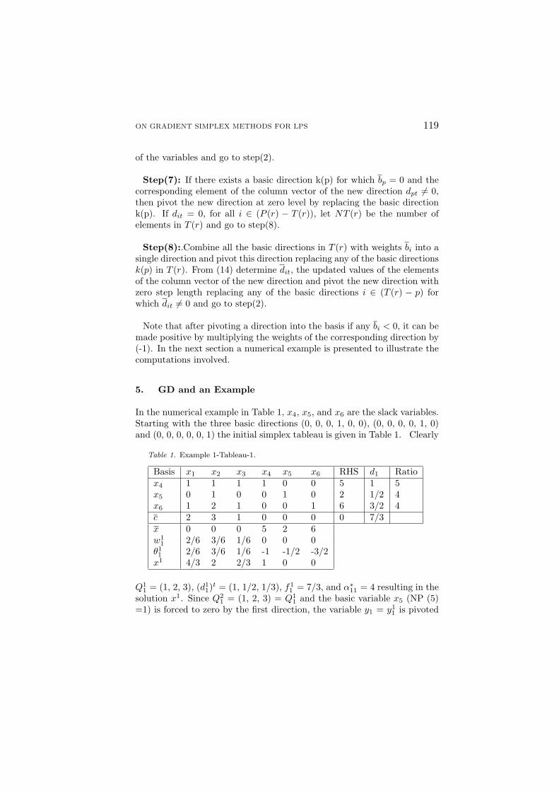
In the numerical example in Table 1, x4, x5, and x6 are the slack variables.Starting with the three basic directions (0, 0, 0, 1, 0, 0), (0, 0, 0, 0, 1, 0)and (0, 0, 0, 0, 0, 1) the initial simplex tableau is given in Table 1. Clearly

Table 1. Example 1-Tableau-1.

Basis x1 x2 x3 x4 x5 x6 RHS d1 Ratiox4 1 1 1 1 0 0 5 1 5x5 0 1 0 0 1 0 2 1/2 4x6 1 2 1 0 0 1 6 3/2 4c 2 3 1 0 0 0 0 7/3x 0 0 0 5 2 6w1

1 2/6 3/6 1/6 0 0 0θ11 2/6 3/6 1/6 -1 -1/2 -3/2

x1 4/3 2 2/3 1 0 0

Q11 = (1, 2, 3), (d1

1)t = (1, 1/2, 1/3), f1

1 = 7/3, and α∗11 = 4 resulting in thesolution x1. Since Q2

1 = (1, 2, 3) = Q11 and the basic variable x5 (NP (5)

=1) is forced to zero by the first direction, the variable y1 = y11 is pivoted

120 R. R. VEMUGANTI

with step length α∗ = 4 replacing x5 in Table 1 (x6 could also have beenreplaced) resulting in Table 2.

Table 2. Example 1 -Tableau-2.

Basis x1 x2 x3 x4 x5 x6 RHS d2 Ratiox4 1 -1 1 1 -2 0 1 1 1y1 0 2 0 0 2 0 4 -5/7 -x6 1 -1 1 0 -3 1 0 1 0c 2 -5/3 1 0 -14/3 0 28/3 5/3 -x 4/3 2 2/3 1 0 0w1

2 6/14 -5/14 3/14 0 0 0θ12 2/3 0 1/3 -1 0 -1

x1 4/3 2 2/3 1 0 0

Since Q12 = (1, 2, 3), it follows that (d1

2)t = (1, -5/7, 1) and f1

2 = 5/3.Clearly α∗21 = 0 due to the basic variable x6 with NP(6) = 1. Replacingx6 with y2 results in Table 3.

Table 3. Example 1-Tableau -3.

Basis x1 x2 x3 x4 x5 x6 RHS d3 Ratiox4 0 0 0 1 1 -1 1 3/10 10/3y1 5/7 9/7 5/7 0 -1/7 5/7 4 -4/35 -y2 1 -1 1 0 -3 1 0 -1 -c 1/3 0 -2/3 0 1/3 -5/3 28/3 7/15 -x 4/3 2 2/3 1 0 0w1

3 1/4 0 -2/4 0 1/4 0θ13 3/4 -1/4 -1/4 -1/4 1/4 0

x1 10/3 4/3 0 1/3 2/3 0w2

3 1/2 0 0 0 1/2 0θ23 5/6 -1/2 1/6 -1/2 1/2 0

x2 35/9 1 1/9 0 1 0

From Table 3, Q13 = (1, 3, 5), (d1

3)t = (1/4, -3/14, -1), f1

3 = 1/2, andα∗31 = 8/3 resulting in the solution x1. From x1 it is clear that Q2

3 = (1, 5)6= Q1

3, (d23)

t = (1/2, 2/7, -1), f23 = 1/3 and α∗32 = 2/3 resulting in x2. Since

the next direction yields Q33 = (1, 3, 5) = Q1

3, the directions y13 and y2

3 arecombined in to a single direction with weights 8/3 and 2/3 resulting in thedirection y3 with weights 8/3w1

3 + 2/3w23. Normalizing (dividing by λ =

10/3) yields the weights (3/10, 0, -4/10, 0, 3/10, 0). The column vectorcorresponding to this direction d3 = 3/10(8/3 d1

3 + 2/3 d23) is shown in

the Table 3. The step length of this direction is λ = 10/3 which forces the


basic variable x4 to zero. Since NP(4) = 1, replacing x4 with y3 results inTable 4.


Basis x1 x2 x3 x4 x5 x6 RHS d4 Ratioy3 0 0 0 10/3 10/3 -10/3 10/3 10/18 6y1 5/7 9/7 5/7 8/21 5/21 7/21 92/21 92/126 6y2 1 -1 1 10/3 1/3 -7/3 10/3 10/18 6c 1/3 0 -2/3 -14/9 -11/9 -1/9 98/9 1/54 -x 35/9 1 1/9 0 1 0w1

4 3/20 0 -6/20 0 -11/20 0θ14 83/90 0 -83/90 0 0 0

x1 4 1 0 0 1 0w2

4 3/14 0 0 0 -11/14 0θ24 65/63 0 -13/126 0 0 0

From Table 4, Q14 = (1, 3, 5), (d1

4)t = ( -11/6, -5/21, -1/3), f1

4 = 83/90,and α∗41 = 10/83 with the corresponding solution x1. The next directionyields Q2

4 = (1, 5), (d24)

t = (-55/21, -5/147, -2/42), f24 = 65/63 and α∗42= 0.

Discarding the second direction and noting the fact that the first directionforced the nonbasic variable x3 to zero, combine all the basic directions y3,y1, and y2 in which x3 has a nonzero weight and the new direction y1

4 withweights [10/3 +11/6(10/83)], [92/21 + 5/21(10/83)], [10/3 + 1/3(10/83)]and 10/83 resulting in the entering direction y4 with normalized weights(4/6, 1/6, 0, 0, 1/6, 0) and step length γ = 6. The corresponding columnvector d4 is shown in Table 4. Replacing y3 with y4, results in Table 5(note that y1 or y2 could have also been replaced).


Basis x1 x2 x3 x4 x5 x6 RHS d5 Ratioy4 0 0 0 6 6 -6 6 -24/5 -y1 5/7 9/7 5/7 -4 -29/7 33/7 0 121/35 0y2 1 -1 1 0 -3 1 0 13/15 0c 1/3 0 -2/3 -5/3 -4/3 0 11 17/15 -x 4 1 0 0 1 0w1

5 1/5 0 0 0 -4/5 0θ15 17/15 0 -17/15 0 0 0

The next possible direction is Q15 = (1, 5) yields α∗51 = 0, due to the

nonbasic variable x3. Noting the fact that P(3) = (2,3) and T(3) = ∅,

122 R. R. VEMUGANTI

replacing y1 with y5 = y15 , yields Table 6 (note that y2 could also have

been replaced).

Table 6. Example 1 -Tableau-6.

Basis x1 x2 x3 x4 x5 x6

y4 120/121 216/121 120/121 54/121 30/121 66/121y5 25/121 45/121 25/121 -140/121 -145/121 165/121y2 56/121 -238/121 56/121 364/121 14/121 -308/121c 12/121 -51/121 -109/121 -43/121 3/121 -187/121x 4 1 0 0 1 0w1

6 4/22 -17/22 0 0 1/22 0θ16 459/113 0 -459/ 113 0 0 0

Basis RHS d6 Ratioy4 6 -1581/ 113 -y5 0 -405 / 113 -y2 0 2142 / 113 0c 11 459 / 113 -

Clearly Q16 = (1, 2, 5) results in α∗61 = 0 due to the nonbasic variable

x3. Since T(3) = ∅, replacing y2 with the direction y6 = y16 , results in the

optimal Table 7.


Basis x1 x2 x3 x4 x5 x6 RHSy4 4/3 1/3 4/3 8/3 1/3 4/3 6y5 5/17 0/17 5/17 -10/17 -20/17 15/17 0y6 44/153 -187/153 44/153 286/153 11/153 -242/153 0c 0 0 -1 -1 0 -1 11x 4 1 0 0 1 0 -

6. Enhancements for the GD Simplex Method

Pivoting a new direction into the basis may result in forcing a variable xr

to zero for which NP(r) ≥ 2 in step(6). In steps 7 and 8, the step lengthof a new direction is restricted to zero with no improvement in the objec-tive function due to a variable at zero level. If P (r) 6= ∅ for the variabledriven to zero, it may be desirable to eliminate this variable from all basicdirections (make the weights to zero). If this is not done, one may have toremove each basic direction in P(r), one at a time resulting in generating


and pivoting several new directions requiring substantial computational ef-fort. The following analysis is directed at developing efficient proceduresand conditions for feasibility of eliminating a variable driven to zero fromall basic directions. There are two cases.

CASE 1: New Direction Step Length α∗ > 0

If xr is basic and NP(r) = 1, the basic direction is replaced by the newdirection with zero weight for xr and therefore the weight of this variable iszero in all basic directions. If xr is nonbasic and NP(r) =1, the new direc-tion is combined with the unique direction in P(r) generating the enteringdirection with zero weight for xr to replace the basic direction k(r) in P(r)resulting in zero weights for xr in all basic directions ( see Lemma(3) andCorollary(2)). Now suppose that xr is basic and NP (r) ≥ 2. If the cor-responding RHS of this basic variable br 6= 0, then the entering directionwith zero weight for xr can be pivoted replacing the basic direction k(r).This makes xr nonbasic and it still has nonzero weights in other basic di-rections. But when br = 0, it is not possible to replace the basic directionk(r). However, since the column corresponding to xr is an identity columnand the value of this variable is zero after pivoting, the weights of the vari-able xr can be made to zero without impacting the identity columns of theother basic variables. The changes needed are to normalize the weights ofthe other basic directions by replacing wjk(i) with wjk(i) / wrk(i) for i 6= rand j 6= r and wrk(i) = 0 for i 6= r and replace the RHS of the basic direc-tions from bi to biwrk(i) (note that wrk(i) 6= 0) where wrk(i) = 1- |wrk(i)|.This reduces the problem to eliminating a nonbasic variable at zero levelwith NP (r) ≥ 1 from all basic directions. Making the weights wrk(i) ofthe nonbasic variable xr to zero changes the identity columns of the basicvariable k(p) for p = (1, . . . ,m) to

gip = −airwrk(p)/wrk(p) fori 6= p

gii = (1− airwrk(i))/wrk(i).

Also the c values of the basic variables are changed from zero to cp =−crwrk(p) / wrk(p). Making the columns of the basic variables to identitycolumns is equivalent to multiplying the matrix A = (aij) with the inverseof the matrix G = (gip). In addition the c values of the basic variablesmust be made to zero. Finally the RHS of the tableau is also changed tobp wrk(p) from bp. The following results provide the inverse of the matrix

124 R. R. VEMUGANTI

G and the condition when it exists and the justification for changing thebp and cp values of the basic variables.

Theorem 6 The inverse of the matrix G, G−1 exists if ∆ = 1 -∑m

i=1 airwrk(i)

6= 0 and the elements of the matrix G−1 = (gpj) are given by

gpj = aprwrk(j)wrk(p)/∆ forp 6= j

gjj = (1 + ajrwrk(j)/∆)wrk(j).

Proof: It is straight forward to verify the result by multiplying the ithrow of the matrix G with the jth column of the matrix G−1.

Lemma 7 When the variable xr is removed from all basic directions andthe remaining weights are normalized, the cp values of the basic variablesare changed to cp = −crwrk(p)/wrk(p).

Proof: Before the variable xr is removed from all basic directions, the cvalues of the basic variables are given by cp =

∑nj=1 wjk(p)cj = 0. Deleting

the weight wrk(p) and normalizing the remaining weights changes the valueto cp =

∑j 6=r cjwjk(p)/wrk(p) = -crwrk(p) / wrk(p).

Lemma 8 When the columns of the x-variables are multiplied by the matrixG−1, the RHS of the tableau is changed to biwrk(i).

Proof: The proof is straight forward by multiplying G−1 and the columnvector of the RHS of the tableau.

To eliminate the weights of the variable xr, from all basic directions firstmultiply the tableau by G−1. Then multiply the pth row of the tableauwith −cp( see Lemma(7)) and add it to the c row for all p to make thecp of the basic variables to zero. Finally change the weights of the basicdirections and the RHS to wjk(p)/wrk(p) and bpwrk(p).

CASE 2 : New Direction Step Length α∗ = 0

The analysis is similar to the case when the step length α∗ > 0 in allsituations except when xr is basic, the corresponding bk(r) 6= 0 and NP(r)≥ 2. In this case combine all basic directions in T(r) ( note that T(r) 6= ∅),with weights bi for i ∈ T (r) as in step (8) and pivot this direction replacingany direction in T(r), except the basic variable xr. This will make bk(r) = 0in the updated tableau. Now the variable xr can be eliminated from allbasic directions except k(r) as discussed in the case when α∗ > 0. Evenbefore pivoting the new direction, it may be possible to remove the variable


xr which caused the zero step length from all basic directions. This mayhelp to reduce the number of pivots with zero step length.To illustrate the computations involved consider the example of the previ-ous section. In the first three tableaus a basic variable is forced to zero.But in Table 4 the entering direction with step length 10/83 forced thenonbasic variable x3 to zero. After the new direction is combined with allbasic directions in P(3) = (1, 2, 3) and pivoting this direction resulted inTable 5. The elements of the column vector of x3 in Table 5 are a13 = 0,a23 = 5/7, and a33 = 1 . Also the weights of x3, in the three basic direc-tions are w3k(1) = 0, w3k(2) = 1/6 and w3k(3) = 3/14. The matrix G andits inverse G−1 are given by

1 0 0 1 0 0G = 0 37/35 -15/77 G−1 = 0 55/36 75/392

0 -1/5 1 0 11/56 407/392

Removing the variable x3 from all basic directions changes the c values ofthe three basic variables to cy4 = 0, cy2 = 2/15 and cy2 = 2/11. Multiply-ing the columns of the x-variables of Table 5 with G−1 and then multiplyingthe rows of the Table 5 with 0, (-2/15) and (-2/11) and adding them to thec row results in the optimal tableau below (Table 8).

Table 8. Example 2 -Optimal Tableau.

Basis x1 x2 x3 x4 x5 x6 RHSy4 0 0 0 6 6 -6 6y1 25/28 30/28 25/28 -110/28 -130/28 135/28 0y2 33/28 -22/28 33/28 -22/28 -110/28 55/28 0c 0 0 -1 -1 0 -1 11

7. Expanded Basis Gradient Simplex Method

In steps (6) of the algorithm a new direction is combined with all basicdirections in P(r) before it can be pivoted into the basis. In step (8),all basic directions in T(r) are combined into a single direction and it ispivoted to make room to pivot the new direction with zero step length.A possible approach to avoid combining the basic directions or combiningwith the basic directions is to expand the basis size. As noted earlier, if thevariable xrwhich is forced to zero is a basic variable and NP(r) = 1, then the

126 R. R. VEMUGANTI

direction can be pivoted replacing xr. Otherwise consider the relationshipur - xr -

∑i∈P (r) wrk(i)yi = 0, where yi are the basic directions pivoted

into the basis so far. Clearly ur yields the value of the variable xr and is aredundant constraint. Adjoin this constraint at the bottom of the tableauwhich increases the size of the basis by one. Suppose the current basis isv ≥ m. Noting the fact that yi = bk(i) -

∑nj=1 ak(i)jxj and substituting for

yi in the expression for ur yields the coefficient av+1j of xj and is given byav+1j =

∑i∈P (r) aijwrk(i) if j 6= r and av+1r =

∑i∈P (r) airwrk(i) − 1.

Theorem 7 The element of the column vector of the entering directioncorresponding to the new constraint dv+1t = - θr.

Proof: By definition

dv+1t =n∑

j=1

wjtav+1j =n∑

j=1

wjt

∑i∈P (r)

aijwrk(i) − wrt

=∑

i∈P (r)

wrk(i)

n∑j=1

ajtwjt − wrt =∑

i∈P (r)

wrk(i)dit − wrt

= −θr.

This proves the required result.Since the RHS of the equation for ur is

∑i∈P (r) biwrk(i) = xr, the variable

ur can be replaced by the new direction with step length α∗. The variableur is discarded after pivoting the new direction. The computations involvedare illustrated using the example of section(6). Since the basic variablesx5, x6 and x4 are forced to zero in the first three iterations, the first fourtableaus generated under both the methods are identical. In Table 4 sincea nonbasic variable x3 is forced to zero, the basis size is expanded form 3 to4 to include the constraint u3 - x3-1/6y1 -3/14y2 + 4/10y3 = 0, where 1/6,3/14 and -4/10 are the weights of the variable x3 in the basic directions y1,y2 and y3. Now substituting for the basic directions y1, y2 and y3 whichare given by

y1 = 92/21− 5/7x1 − 9/7x2 − 5/7x3 − 8/21x4 − 5/21x5 − 7/21x6

y2 = 10/23− x1 + x2− x3− 10/3x4 − 1/3x5 + 7/3x6

y3 = 10/3− 10/3x4 − 10/3x5 + 10/3x6

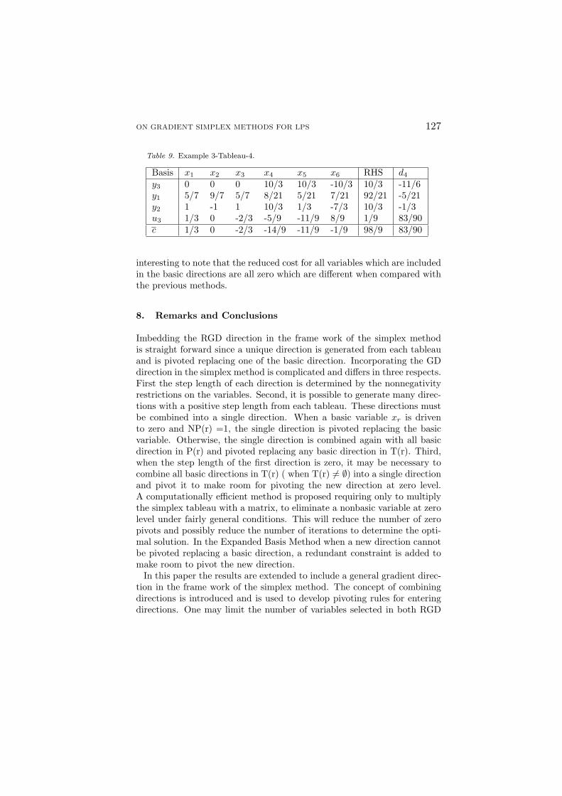
from Table 4, results in u3 +1/3x1 -2/3x3 -5/9x4 -11/9x5 +8/9x6 = 1/9and the following Table 9.

Pivoting y4 and replacing u3 yields the optimal tableau with c = (0,0,0,-1,0,-1), y1 = 366/83, y2 = 280/83, y3 = 295/83, and y4= 10/83. It is



Basis x1 x2 x3 x4 x5 x6 RHS d4

y3 0 0 0 10/3 10/3 -10/3 10/3 -11/6y1 5/7 9/7 5/7 8/21 5/21 7/21 92/21 -5/21y2 1 -1 1 10/3 1/3 -7/3 10/3 -1/3u3 1/3 0 -2/3 -5/9 -11/9 8/9 1/9 83/90c 1/3 0 -2/3 -14/9 -11/9 -1/9 98/9 83/90

interesting to note that the reduced cost for all variables which are includedin the basic directions are all zero which are different when compared withthe previous methods.

8. Remarks and Conclusions

Imbedding the RGD direction in the frame work of the simplex methodis straight forward since a unique direction is generated from each tableauand is pivoted replacing one of the basic direction. Incorporating the GDdirection in the simplex method is complicated and differs in three respects.First the step length of each direction is determined by the nonnegativityrestrictions on the variables. Second, it is possible to generate many direc-tions with a positive step length from each tableau. These directions mustbe combined into a single direction. When a basic variable xr is drivento zero and NP(r) =1, the single direction is pivoted replacing the basicvariable. Otherwise, the single direction is combined again with all basicdirection in P(r) and pivoted replacing any basic direction in T(r). Third,when the step length of the first direction is zero, it may be necessary tocombine all basic directions in T(r) ( when T(r) 6= ∅) into a single directionand pivot it to make room for pivoting the new direction at zero level.A computationally efficient method is proposed requiring only to multiplythe simplex tableau with a matrix, to eliminate a nonbasic variable at zerolevel under fairly general conditions. This will reduce the number of zeropivots and possibly reduce the number of iterations to determine the opti-mal solution. In the Expanded Basis Method when a new direction cannotbe pivoted replacing a basic direction, a redundant constraint is added tomake room to pivot the new direction.

In this paper the results are extended to include a general gradient direc-tion in the frame work of the simplex method. The concept of combiningdirections is introduced and is used to develop pivoting rules for enteringdirections. One may limit the number of variables selected in both RGD

128 R. R. VEMUGANTI

and GD directions without significant changes in the proposed methods.The motivation for limiting the number of variables is that an optimal solu-tion can always be found with no more that m variables at a positive level.The feasibility of reducing the basis size in the Expanded Basis Methodand computational experiments for the two methods presented are underinvestigation.

Acknowledgments

The author is grateful to anonymous referees and the area editor for con-structive comments on earlier version of this paper and to a colleague Dr.Danielle Fowler for help with the Latex Package.

References

1. P. Abel. On the Choice of the Pivot Columns of the Simplex Method: GradientCriteria. Computing,13: 13-21, 1987.

2. K. M. Anstreicher and T. Terlaky. A Monotonic Build-up Simplex Algorithm forLinear Programming. Operations Research, 48: 556-561, 1994.

3. M. H. Beilby. Economics and Operations Research. Academic Press, 25-41, 1976.4. R. G. Bland. New Finite Pivoting Rules for the Simplex Method. Mathematics of

Operations Research, 2: 103-107, 1977.

5. H- D. Chen, P. M.. Pardalos and M.. A. Saunders. The Simplex Algorithm with aNew Primal and Dual Pivot Rule. Operations Research Letters, 16: 121-127, 1994.

6. M. C. Cheng. Generalized Theorems for Permanent Basic and Nonbasic Variables.Mathematical Programming, 31: 229-234, 1985.

7. G. B. Dantzig. Linear Programming and Extensions. Princeton University Press,Princeton, New Jersey, 1963.

8. H. A. Eiselt and C- L. Sandblom. Experiments with External Pivoting. Computersand Operations Research, 17: 325-332,1990.

9. Y. Fathi and K. G. Murty. Computational Behavior of a Feasible Direction Methodfor Linear Programming. European Journal of Operational Research,40: 322-328,1989.

10. P. E. Gill, W. Murray, M. A. Saunders, and M. A. Wright. A Practical Anti-CyclingProcedure for Linearly Constrained Optimization. Mathematical Programming, 45:437-474,1989.

11. D. Goldfarb and J. K. Reid. A Practicable Steepest-Edge Simplex Algorithm.Mathematical Programming, 12: 361-371, 1977.

12. R. L. Graves and P. Wolfe. Recent Advances in Mathematical Programming.McGraw-Hill, New York, San Francisco, Toronto, London, 76-77, 1964.

13. P. M. J. Harris. Pivot Selection Methods of the Devex LP Code. MathematicalProgramming, 5: 1-28, 1973.

14. E. O. Heady and W. Candler. Linear Programming Methods. The Iowa StateCollege Press, Ames, 560-563, 1958.

15. M. Kallio and E. L. Porteus. A Class of Methods for Linear Programming. Math-ematical Programming, 14: 161-169, 1978.


16. B. Kreko. Linear Programming (Translated by J.H.L. Ahrens and C.M. Safe). SirIssac Pitman & Sons, London, 258-271, 1968.

17. G. Mitra, M..Tamiz and J. Yadegar. A Hybrid Algorithm For Linear Programs.em Simulation and Optimization of Large Systems, Edited By A. J. Osiadacz,Clarendon Press, Oxford, 1988.

18. S. R. Paranjape. The Simplex Method: Two Basic Variables Replacement. Man-agement Science, 12: 135-141, 1965.

19. J. B. Rosen. The Gradient Projection Method for Nonlinear Programming - PartI: Linear Constraints. Journal of Society of Industrial and Applied Mathematics,9: 181-217, 1961.

20. T. Terlaky and S. Zhang. Pivot Rules for Linear Programming: A Survey on RecentTheoretical Developments. Annals of Operations Research, 46: 203-233, 1993.

21. Y. Ye. Eliminating Columns in the Simplex Method for Linear Programming.Journal of Optimization Theory and Applications, 63: 69-77, 1989.

22. S. Zhang. On Anti-Cycling Pivoting Rules for the Simplex Method. OperationsResearch Letters, 10: 189-192, 1992.

23. P. H. Zipkin. Bounds on the Effect of Aggregating Variables in Linear Programs.Operations Research, 28: 403-418, 1980.

24. G. Zoutendijk Mathematical Programming Models. North Holland PublishingCompany, Amsterdam, New York, Oxford, 99-115, 1976

Mathematical Problems in Engineering

Special Issue on

Time-Dependent Billiards

Call for PapersThis subject has been extensively studied in the past yearsfor one-, two-, and three-dimensional space. Additionally,such dynamical systems can exhibit a very important and stillunexplained phenomenon, called as the Fermi accelerationphenomenon. Basically, the phenomenon of Fermi accelera-tion (FA) is a process in which a classical particle can acquireunbounded energy from collisions with a heavy moving wall.This phenomenon was originally proposed by Enrico Fermiin 1949 as a possible explanation of the origin of the largeenergies of the cosmic particles. His original model wasthen modified and considered under different approachesand using many versions. Moreover, applications of FAhave been of a large broad interest in many different fieldsof science including plasma physics, astrophysics, atomicphysics, optics, and time-dependent billiard problems andthey are useful for controlling chaos in Engineering anddynamical systems exhibiting chaos (both conservative anddissipative chaos).

We intend to publish in this special issue papers reportingresearch on time-dependent billiards. The topic includesboth conservative and dissipative dynamics. Papers dis-cussing dynamical properties, statistical and mathematicalresults, stability investigation of the phase space structure,the phenomenon of Fermi acceleration, conditions forhaving suppression of Fermi acceleration, and computationaland numerical methods for exploring these structures andapplications are welcome.

To be acceptable for publication in the special issue ofMathematical Problems in Engineering, papers must makesignificant, original, and correct contributions to one ormore of the topics above mentioned. Mathematical papersregarding the topics above are also welcome.

Authors should follow the Mathematical Problems inEngineering manuscript format described at http://www.hindawi.com/journals/mpe/. Prospective authors shouldsubmit an electronic copy of their complete manuscriptthrough the journal Manuscript Tracking System at http://mts.hindawi.com/ according to the following timetable:

Manuscript Due December 1, 2008

First Round of Reviews March 1, 2009

Publication Date June 1, 2009

Guest Editors

Edson Denis Leonel, Departamento de Estatística,Matemática Aplicada e Computação, Instituto deGeociências e Ciências Exatas, Universidade EstadualPaulista, Avenida 24A, 1515 Bela Vista, 13506-700 Rio Claro,SP, Brazil ; [email protected]

Alexander Loskutov, Physics Faculty, Moscow StateUniversity, Vorob’evy Gory, Moscow 119992, Russia;[email protected]

Hindawi Publishing Corporationhttp://www.hindawi.com

http://www.hindawi.com/journals/mpe/

http://www.hindawi.com/journals/mpe/

http://mts.hindawi.com/

http://mts.hindawi.com/

on gradient simplex methods for linear programs · on gradient simplex methods for linear ......

Documents