master of engineering ocean & naval architectural

INFLUENCE OF BRIDGE OFFICER EXPERIENCE ON ICE MANAGEMENT

EFFECTIVENESS

By Erik Veitch

A thesis submitted to the School of Graduate Studies in partial fulfillment of the

requirements for the degree of

Master of Engineering

Ocean & Naval Architectural Engineering

Engineering & Applied Science

Memorial University of Newfoundland

August 2018

St. John’s, Newfoundland & Labrador

ii

ABSTRACT

The research presented in this thesis investigates the influence of human expertise on the

effectiveness of ice management operations. This was accomplished in an experiment

using a marine simulator in which 36 participants with a range of seafaring experience

levels were tasked with individually completing ice management exercises. Effectiveness

was assessed in terms of the operator’s ability to lower pack ice concentration around an

offshore structure and to keep a defined area free of ice for a lifeboat launch. These

responses were compared to two independent variables: i) experience level of the

participant, and ii) ice concentration. The results showed a significant difference in ice

management effectiveness between experience categories. Characterizations of effective

ice management techniques were presented based on the results. This result has

implications for training in the nautical sciences and can help inform best practices in ice

management.

iii

ACKNOWLEDGEMENTS

The author gratefully acknowledges the financial support provided by Natural

Sciences and Engineering Research Council (NSERC) / Husky Energy Industrial Research

Chair in Safety at Sea, and by the American Bureau of Shipping (ABS) Harsh Environment

Technology Centre. The author also acknowledges with gratitude the financial support

provided by the Research and Development Corporation (RDC) Ocean Industry Student

Research Award.

The author would like to personally thank the generous support of Dr. Leonard Lye,

whose willingness to teach graduate students about experimental design is the only the

thing that exceeds his knowledge of the subject area.

The author would also like to thank Brian MacDonald, a co-operative education

student whom we hired to assist during experimental trials, and whose assistance proved

invaluable (despite having fallen asleep in the simulator during one particularly slow

morning).

The author would also like to thank Jennifer Smith, whose tremendous ability to

manage volunteer participants made the experimental campaign a success, as well as Sean

Jessome, whose last-minute bug fixes to the simulator saved the day more than once.

Lastly, I would like to thank the wonderful staff at Fixed Café on Duckworth Street,

St. John’s, for serving me hundreds of small black coffees while I wrote this thesis.

iv

TABLE OF CONTENTS

ABSTRACT ........................................................................................................................ ii

ACKNOWLEDGEMENTS ............................................................................................... iii

TABLE OF CONTENTS ................................................................................................... iv

LIST OF TABLES ............................................................................................................. vi

LIST OF FIGURES .......................................................................................................... vii

LIST OF ABREVIATIONS AND SYMBOLS ...................................................................x

INTRODUCTION ...............................................................................................................1

1 Literature Review .........................................................................................................3

2 Methods ........................................................................................................................7

2.1 Simulator ............................................................................................................. 7

2.2 Design of Experiments ...................................................................................... 11

2.3 Analysis ............................................................................................................. 14

3 Results ........................................................................................................................16

3.1 Average Clearing .............................................................................................. 20

3.2 Peak Clearing .................................................................................................... 28

3.3 Total Clearing ................................................................................................... 32

3.4 Clearing-to-Distance Ratio ............................................................................... 37

v

3.5 Ice-Free Lifeboat Launch Time ........................................................................ 43

3.6 Ice Management Tactics ................................................................................... 50

4 Discussion and Future Work ......................................................................................57

5 Conclusions ................................................................................................................62

6 REFERENCES ..........................................................................................................64

7 Appendices .................................................................................................................69

7.1 Power Analysis and Experiment Sizing ............................................................ 69

7.2 Diagnostics Plots ............................................................................................... 75

7.2.1 Diagnostics Plots for Peak Clearing Metric ................................................ 75

7.2.2 Diagnostics Plots for Total Clearing Metric ............................................... 77

7.2.3 Diagnostic Plots for Clearing-to-Distance Ratio Metric ............................. 78

7.2.4 Diagnostic Plots for Ice-Free Lifeboat Launch Time Metric ...................... 79

vi

LIST OF TABLES

Table 1: Descriptive statistics for cadets’ average clearing (tenths concentration) .................................... 20

Table 2: Descriptive statistics for seafarers’ average clearing (tenths concentration) ............................... 20

Table 3: REML ANOVA (average clearing) ................................................................................................. 24

Table 4: REML variance components table ................................................................................................. 24

Table 5: Descriptive statistics for cadets’ peak clearing (tenths concentration) ......................................... 28

Table 6: Descriptive statistics for seafarers’ peak clearing (tenths concentration) ..................................... 28

Table 7: REML ANOVA (peak clearing in “Emergency” scenario) ............................................................ 31

Table 8: Descriptive statistics for cadets’ total clearing (km2) .................................................................... 33

Table 9: Descriptive statistics for seafarers’ total clearing (km2)................................................................ 33

Table 10: REML ANOVA (total clearing for “Emergency” scenario) ......................................................... 35

Table 11: Total distance travelled (km)........................................................................................................ 37

Table 12: Descriptive statistics for cadets’ clearing-to-distance ratio (km2/km) ......................................... 37

Table 13: Descriptive statistics for seafarers’ clearing-to-distance ratio (km2/km) .................................... 38

Table 14: REML ANOVA (clearing-to-distance ratio for “Emergency” scenario) ..................................... 40

Table 15: Descriptive statistics for cadets’ cumulative ice-free lifeboat launch times (minutes) ................ 45

Table 16: Descriptive statistics for seafarers’ cumulative ice-free lifeboat launch times (minutes) ............ 45

Table 17: REML ANOVA (cumulative ice-free lifeboat launch time) .......................................................... 47

Table 18: Inputs for prospective power analysis based on 2-sample t-test .................................................. 70

Table 19: Results of prospective power analysis for 2-sample t-test ............................................................ 71

Table 20: Inputs for retrospective / post-hoc power analysis based on 2-sample t-test ............................... 73

vii

LIST OF FIGURES

Figure 1: Schematic of the simulator set-up ................................................................................................... 7

Figure 2: Schematic of the simulator bridge console ..................................................................................... 8

Figure 3: Screenshot from the Instructor Station monitor during simulation. ............................................. 10

Figure 4: “Precautionary” ice management scenario (7-tenths) ................................................................ 13

Figure 5: “Emergency” ice management scenario (7-tenths) ..................................................................... 14

Figure 6: Example measurements from a single simulation trial ................................................................. 17

Figure 7: The example case with three performance metrics illustrated ..................................................... 19

Figure 8: Boxplots of average ice clearing for “Emergency” scenario ....................................................... 21

Figure 9: Half-normal plot of subplot effects ............................................................................................... 23

Figure 10: Half-normal plot of whole-plot effects........................................................................................ 23

Figure 11: Interaction plot of concentration and experience on average clearing. ..................................... 25

Figure 12: Normal plot of residuals ............................................................................................................. 27

Figure 13: Residuals versus predicted values .............................................................................................. 27

Figure 14: Residuals versus run order ......................................................................................................... 27

Figure 15: Box-Cox plot for power transform ............................................................................................. 27

Figure 16: Boxplots of peak ice clearing for “Precautionary” scenario ..................................................... 30

Figure 17: Boxplots of peak ice clearing for “Emergency” scenario .......................................................... 30

Figure 18: Boxplots of total ice clearing for “Emergency” scenario .......................................................... 34

Figure 19: Interaction plot of concentration and experience on total ice clearing ...................................... 36

Figure 20: Boxplots of clearing-to-distance ratio for “Emergency” scenario ............................................ 39

viii

Figure 21: Main effect plot of clearing-to-distance ratio versus experience ............................................... 41

Figure 22: Box-Cox plot for power transform (clearing-to-distance ratio model) ...................................... 42

Figure 23: Port lifeboat launch zone (not to scale)...................................................................................... 44

Figure 24: Boxplots of cumulative ice-free lifeboat launch times during “Emergency” scenario .............. 46

Figure 25: Main effect plot of cumulative ice-free lifeboat launch time versus experience ......................... 48

Figure 26: Box-Cox plot for power transform (cumulative ice-free lifeboat launch time model) ................ 49

Figure 27: Heatmap for cadets’ tracks during “Emergency” scenario ....................................................... 51

Figure 28: Heatmap for seafarers’ tracks during “Emergency” scenario .................................................. 51

Figure 29: Plot of best and worst tracks for “Emergency” scenario. .......................................................... 54

Figure 30: Midway mark (15 min) during “Emergency” scenario for best trial .......................................... 54

Figure 31: Midway mark (15 min) during “Emergency” scenario for worst trial ...................................... 54

Figure 32: Plot of actual versus self-reported performance scores with LOESS line .................................. 61

Figure 33: Prospective power curve for 2-sample t-test .............................................................................. 72

Figure 34: Retrospective / post-hoc power curve for 2-sample t-test........................................................... 74

Figure 35: Normal plot of residuals (peak clearing) ................................................................................... 75

Figure 36: Residuals versus predicted values (peak clearing) ..................................................................... 75

Figure 37: Residuals versus run order (peak clearing) ............................................................................... 76

Figure 38: Box-Cox plot for power transform (peak clearing) .................................................................... 76

Figure 39: Normal plot of residuals (total clearing) .................................................................................... 77

Figure 40: Residuals versus predicted values (total clearing) ..................................................................... 77

Figure 41: Residuals versus run order (total clearing) ................................................................................ 77

Figure 42: Box-Cox plot for power transform (total clearing) .................................................................... 77

ix

Figure 43: Normal plot of residuals (clearing-to-distance ratio) ................................................................ 78

Figure 44: Residuals versus predicted values (clearing-to-distance ratio) ................................................. 78

Figure 45: Residuals versus run order (clearing-to-distance ratio) ............................................................ 78

Figure 46: Box-Cox plot for power transform (clearing-to-distance ratio) ................................................. 78

Figure 47: Normal plot of residuals (ice-free lifeboat launch time) ............................................................ 79

Figure 48: Residuals versus predicted values (ice-free lifeboat launch time).............................................. 79

Figure 49: Residuals versus run order (ice-free lifeboat launch time) ........................................................ 79

Figure 50: Box-Cox plot for power transform (ice-free lifeboat launch time) ............................................. 79

x

LIST OF ABREVIATIONS AND SYMBOLS

AHTS Anchor Handling Tug Supply

ANOVA Analysis of Variance

CRD Completely Random Design

DP Dynamic Positioning

FPSO Floating, Production, Storage and Offloading

GPS Global Positioning System

IMO International Maritime Organization

LOESS Locally Weighted Scatterplot Smoothing

LSD Least Significant Difference

OSV Offshore Supple Vessel

REML Restricted Maximum Likelihood

STCW Standards of Training, Certification and Watchkeeping for Seafarers

TEMPSC Totally Enclosed Motor Propelled Survival Craft

AZ Area of ice management zone

Ci Incremental concentration drop

Δt Sampling interval

1

INTRODUCTION

Expertise of human operators plays an important role in ice management

operations, which rely heavily on the knowledge and proficiency of individuals

orchestrating operations from the bridge of support vessels. It follows that expertise of

bridge officers may distinguish one individual from another in terms of ice management

effectiveness. Despite its importance, though, expertise is rarely included in engineering

assessments, mainly due to the difficulty it poses in terms of assessment. In this research,

the influence of expertise of bridge officers in ice management is quantified. Systematic

investigation was made possible with the use of a full-mission marine simulator.

The influence of two factors on the effectiveness of ice management operations was

studied: i) bridge officer experience and ii) ice severity. It was hypothesized that ice

management would be more effective (that is, more ice would be cleared in a given amount

of time) with more experienced bridge officers compared to novice ones. Furthermore, it

was hypothesized that this experience effect would be stronger in more severe ice

conditions (higher ice concentrations).

The context of the research question is important for marine industry operators in

areas where sea ice and glacial ice must be managed to enable operations to proceed safely

[1], [2]. This research investigates the case of drifting broken sea ice when it enters an area

in which a moored, floating installation is present. An experimental campaign was designed

to test the relationship between the human factor of bridge crew experience and the

2

environmental factor of ice concentration on the effectiveness of a defined ice management

operation.

3

1 LITERATURE REVIEW

A marine simulator was used to create a virtual scenario in which drifting broken

sea ice entered an area in which a moored, floating installation was present. Such operations

have been documented for many regions, including the Arctic Ocean [3], the Okhotsk

Sea [4], and the Beaufort Sea [5]. The simulation scenario was used in an experimental

campaign to investigate the influence of bridge officer experience on the effectiveness of

ice management. Ice management has no formal definition, although one definition has

been offered that fits well within the scope of the research discussed herein [1]: “[ice

management is] a systematic operation enabling a main activity that could not be safely

conducted without additional actions due to potential existence of sea ice.” In the simulated

scenario, the main activities are oil production and offloading on a Floating, Production,

Storage & Offloading vessel (FPSO). The stand-by vessel is tasked with enabling this main

activity to proceed safely in the presence of sea ice by, among other things, keeping its port

and starboard lanes clear should lifeboats have to be deployed during a major event.

Several studies have reported how ice loads on structures might be reduced through

ice management measures [6], [7], [8], [9], and [10]. Barker et al. [6] describes a moored

station-keeping vessel in moving pack ice and suggests that reduction of ice severity

through ice management can drastically reduce loads on the mooring lines. Spencer &

Molyneux [7] go one step further, showing that ice concentration, measured in fraction of

coverage, plays a vital role in predicting loads acting on the hull of a moored, floating ship-

shaped structure. Such loads increase exponentially in proportion to ice coverage, with the

notable exception being ice concentrations under 4-tenths coverage, for which insignificant

4

loading is experienced. Considering that most floating production systems located in arctic

and sub-arctic waters will likely encounter small floes drifting freely under environment

forces, the focus on ice concentration as a key predictor of operational success is an

important one and one that will be considered in this research during simulated ice

management scenarios. Level ice has been shown to produce very high loads on moored

structures [10], but remains outside the scope of this research. In terms of operational

procedures in ice management, Hamilton et al. [8] showed that ice management in drifting

pack ice for a station-keeping vessel may take several different forms. Variation in

operational techniques are described as “fleet deployment patterns” and come in a variety

of different techniques ranging from “circular” to “linear.” This suggests that the way in

which ice management is carried out on the bridge of a support vessel plays an important

role in ice management effectiveness, not just according to which technique is employed,

but also to the extent that a given fleet deployment pattern is executed effectively according

to the expertise of the operator in control. Iceberg drift, investigated in [9], also plays a

deciding role in ice management operations in areas where icebergs may be seasonally

present, however in this research ice management simulations do not include icebergs. The

ice that is encountered in the simulations used in this study is based on pack ice typical of

that which may be found seasonally on the Grand Banks of Newfoundland. This pack ice

is first year ice with a thickness of 30 to 70 cm and is composed of small floes in the range

of 20 to 100 m in diameter, drifting at a rate of 0.5 knots [11]. The simulated ship-

interaction is based on PhysX rigid body mechanics software [12], which was initially

developed for computer gaming. This research is not the first time that such a numerical

technique has been used for ship-ice interaction modeling; Lubbad & Loset [13] showed

5

that complex and computationally taxing real-time ship-ice interaction simulations done in

PhysX exhibited satisfactory agreement to full-scale tests. The authors even suggested that

the real-time criterion of such simulations may have applications in training of offshore

personnel in arctic operations, which is the predominant theme of the current research.

The use of marine simulators for training in maritime operations is not a novel

invention. Simulator training is mandated and regulated internationally by the Standards

of Training, Certification and Watchkeeping for Seafarers (STCW). In 2017, the STCW

was amended for training requirements for vessels operating in polar waters, which

includes ice management activities. These requirements reflect regulations described by

the International Maritime Organization’s International Code for Ships Operating in Polar

Waters – known as the “Polar Code” – which came into effect on January 1, 2017. Model

courses were approved by the IMO in the Spring of 2017 to help ensure knowledge transfer

of Polar Code certification requirements to students and to help set the expectations for

training institutions. These model courses highlight marine simulator technology as an

effective means of transferring skills to an individual – should simulators be available. In

academic studies, marine simulators have been shown to be effective tools for training for

operations where the same skills would be costly, resource-intensive, and risky to practice

onboard real vessels [14], [15]. Still, some studies show that simulators are not to be treated

as panacea for training. Some studies have suggested that there is a limit to what can be

experienced in a simulator and that simulator training should be approached with measured

skepticism. For instance, one study suggested that marine operations are so complex on a

spatial and temporal scale and so intricate in terms of socio-technical interactions that

6

recreating them in a simulator may be of limited use in training [16]. The same author also

argues that lack of photorealism can affect seafarers’ learning objectives negatively, since

it may cause trainees to idly navigate the marine simulator environment without meaningful

engagement required for learning [17].

Despite known values and limitations, many questions related to the use of simulators

in maritime training and assessment remain unanswered. A literature review conducted in

2017 showed that few empirical studies have investigated the pedagogical aspects of bridge

officer training in marine simulators [18]. This was impetus for a 2018 study by the same

author, who aimed to investigate the role of instructions and assessments for developing

trainees’ competencies in a simulator-based maritime education program [19]. This was

accomplished with the use of ethnographic fieldwork and analysis of video data. Among

other things, the study showed that good seamanship practice is hard to teach, and that

while instructional support in the forms of monitoring, assessment, and feedback should

form the core of the training program, there is still a lack of understanding of simulator

training and assessment. In other words, the obvious questions of how to design an effective

training program in a marine simulator remains, for the large part, unknown. The work in

this thesis may help to inform this question, specifically in aspects of simulation scenario

design and participants’ assessment in ice management training.

7

2 METHODS

2.1 Simulator

The ice management simulator used in the experiment was designed and built for

research. It uses PhysX software rigid body mechanics computation and simulation

software [12]. The simulator consists of a bridge console positioned in the middle of a 360-

degree panoramic projection screen. The bridge console is a (2 m x 2 m) platform mounted

on a Moog motion bed. For this experiment, the motion bed was turned off. A schematic

of the simulator is shown in Figure 1.

Figure 1: Schematic of the simulator set-up

8

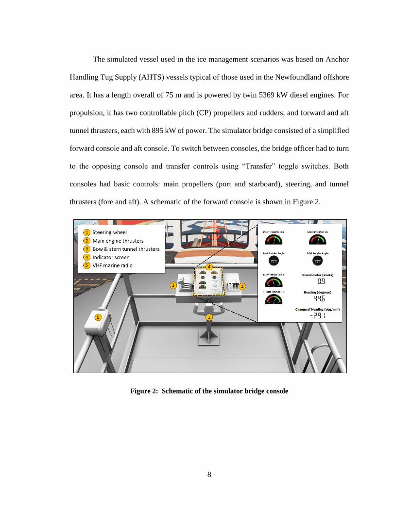
The simulated vessel used in the ice management scenarios was based on Anchor

Handling Tug Supply (AHTS) vessels typical of those used in the Newfoundland offshore

area. It has a length overall of 75 m and is powered by twin 5369 kW diesel engines. For

propulsion, it has two controllable pitch (CP) propellers and rudders, and forward and aft

tunnel thrusters, each with 895 kW of power. The simulator bridge consisted of a simplified

forward console and aft console. To switch between consoles, the bridge officer had to turn

to the opposing console and transfer controls using “Transfer” toggle switches. Both

consoles had basic controls: main propellers (port and starboard), steering, and tunnel

thrusters (fore and aft). A schematic of the forward console is shown in Figure 2.

Figure 2: Schematic of the simulator bridge console

9

The bridge console was highly simplified and did not have navigational

components such as radar, GPS, or chart systems. Moreover, the simulated version of the

AHTS was not exact in hydrodynamic likeness, particularly with regard to its seakeeping

and maneuvering characteristics. Notwithstanding these limitations in similitude, the

simulator was good enough for this experiment whose purpose was to detect differences

between bridge officer experience groups and characterize general principles of good ice

management practices. Face validation of the simulator, conducted prior to the execution

of this study, was completed using feedback from masters and mates operating similar

AHTS vessels to that being simulated.

All participants in the experiment were given 60 minutes to familiarize themselves

with the controls and maneuvering characteristics prior to completing the ice management

scenarios. This was accomplished in three basic 20-minute-long scenarios designed to

habituate participants to the simulation environment. None of the participants had used the

simulator before. Signs and symptoms of simulator-induced sickness were monitored

before and after each exposure period to the simulator using a self-reported questionnaire

[20]. No participants noted simulator sickness symptoms severe enough to justify stopping

a simulation trial.

The Instructor Station was located several meters outside the periphery of the

projection screen, out of view from inside the simulator. This is where the experimenters

started and stopped scenarios and provided scripted instructions to the bridge officer inside

the simulator. Instructions were communicated with a two-way VHF radio. Distances from

the “own-ship” (the vessel being operated in the simulator) to specified targets could also

10

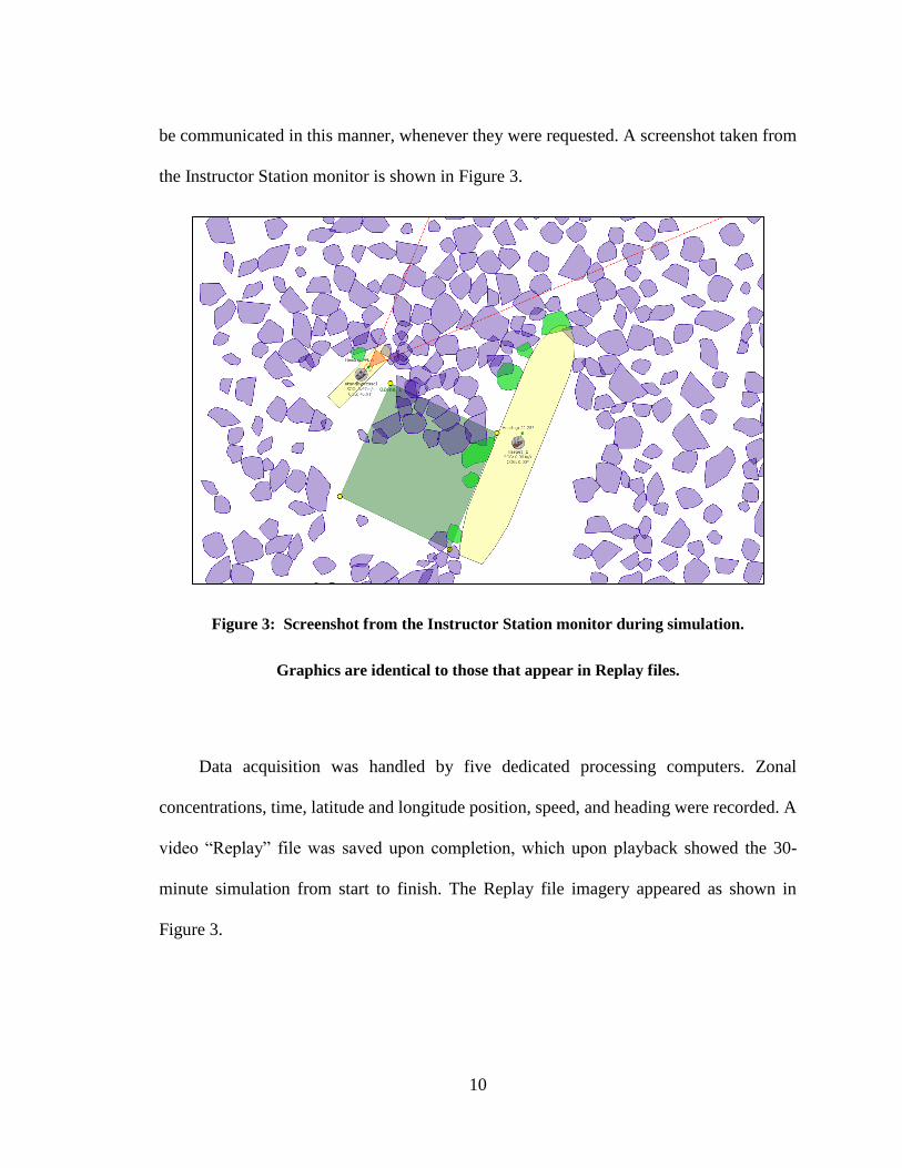
be communicated in this manner, whenever they were requested. A screenshot taken from

the Instructor Station monitor is shown in Figure 3.

Figure 3: Screenshot from the Instructor Station monitor during simulation.

Graphics are identical to those that appear in Replay files.

Data acquisition was handled by five dedicated processing computers. Zonal

concentrations, time, latitude and longitude position, speed, and heading were recorded. A

video “Replay” file was saved upon completion, which upon playback showed the 30-

minute simulation from start to finish. The Replay file imagery appeared as shown in

Figure 3.

11

2.2 Design of Experiments

The approach adopted a formal design of experiments [21]: a 2k full factorial was

completed with nine replicates and k = 2 factors, totaling 36 runs. The first factor, ice

severity, was represented by ice concentration and could be changed in the parameter

settings of the simulator. The low-level treatment was set to 4-tenths ice concentration; the

high-level treatment was set to 7-tenths ice concentration. The second factor, experience

level of bridge officers, was represented by a high- and low-level categorical variable. The

low-level experience category consisted of eighteen cadets enrolled in a local seafaring

program (average years spent at sea from 0-3 years). This group included six students from

each of the 1st, 2nd, and 4th year classes. The high-level experience category consisted of

eighteen seafarers (masters and mates) employed in the marine industry (average years

spent at sea = 20 ± 10 years). This group included operators of coastal ferries, bulk carriers,

cargo tankers, offshore supply vessels (OSVs), and anchor-handling tug supply vessels

(AHTSs), with the latter two subset groups contributing the highest number of participants.

The number of participants was based on a power analysis, whereby an estimate of effect

size and variance in a given response variable was used to estimate the required sample

size at a given statistical power and Type 1 error rate [22]. For the interested reader, more

information about the power analysis procedure used in sizing this experiment is described

in the Appendices (Section 7.1). Participants were recruited on a volunteer basis. Following

the research protocol approved by Memorial University’s interdisciplinary committee on

ethics in human research, all volunteers provided their informed consent before

participating in the experiment.

12

Due to the logistical challenges of scheduling thirty-six voluntary research

participants, it was impractical to run a Completely Random Design (CRD). In standard

experiment designs, the order of individual trials is determined randomly – a method that

usually ensures that observations are independent, thereby complying with statistical

methods. A way to circumvent the problem of restricted randomization is the split-plot

design [23], [24]. In this design, the hard-to-change experience variable stayed constant in

pairs of consecutive runs (the whole-plot) while the easy-to-change concentration variable

was randomly selected for each group (the sub-plot). The experimental error of effects

estimates could thereafter be estimated separately, thereby balancing the biasing effect of

uncontrollable experimental conditions that may have otherwise been undetectable.

Having just two independent variables in the experiment (ice concentration and

experience level) and one dependent variable (concentration reduction), the aim was to use

straightforward scenarios in order to avoid introducing confounding factors. Still, the

scenario had to be a realistic representation of an ice management exercise. Each of the

thirty-six participants completed two different ice management scenarios to reflect

different ice management tasks. The first scenario was called “Precautionary” ice

management, in which the participant was tasked with keeping the area around a moored

FPSO clear of ice. The second scenario was called “Emergency” ice management, in which

the participant was tasked with clearing away ice from an area underneath one of the

FPSO’s lifeboat launch zones in preparation for evacuation. The areas the participants were

tasked with clearing are outlined in Figures 4 and 5. Other than FPSO heading (0 degrees

for the “Precautionary” and 23 degrees for the “Emergency” scenario) and ice

13

concentration (low level 4-tenths and high level 7-tenths), all other conditions in the

scenarios were equivalent. As there were two ice concentration levels and two different ice

management scenarios, there were four different scenarios used in total in this experiment

(the two 7-tenths concentration cases are shown in Figures 4 and 5). Each participant

completed both scenarios at the same ice concentration level. All scenarios were 30 minutes

long. The floe sizes were randomly sampled from a lognormal distribution whose

parameters were based upon input from a subject matter expert during face validation of

the simulator. The floe thickness was uniformly set to 40 cm.

Figure 4: “Precautionary” ice management scenario (7-tenths)

14

Figure 5: “Emergency” ice management scenario (7-tenths)

2.3 Analysis

Five performance metrics were used to assess ice management effectiveness:

i) average ice clearing (tenths concentration), ii) peak ice clearing (tenths concentration),

iii) total ice clearing in a defined area (km2), iv) clearing-to-distance ratio (km2/km) (all

measured in a defined area), and v) cumulative ice-free lifeboat launch time (minutes). The

latter of the five metrics applied to the “Emergency” scenario, only.

15

Analysis of each of the five performance metrics was performed in a similar way.

First, data were explored in a descriptive and visual sense. This was then followed by a

more rigorous approach whose aim was to determine the extent to which ice concentration

and bridge officer experience influenced the effectiveness of the simulated ice management

scenarios. The main effects of each factor and their interaction effect are determined in the

same way as in a regular factorial design. The key difference is that a half-normal plot of

effects was used to screen for significant effects for whole-plot and sub-plot groups

separately [25]. Then ANOVA is used to check for significant effects and accounted for

the group terms separately [26]. Significant effects from both groups are then combined to

give the final model.

Residual plots were used to check modelling assumptions [27]. Diagnostic checks of

modeling adequacy showed that assumptions of normally distributed residuals,

heteroscedasticity, and independence of residuals with run order were. This check was

performed for all analyses in this work because it showed that modelling assumptions were

valid, thereby supporting any inferences on which they were based.

Additional analysis helped to answer the question of what characterized good ice

management practices for particularly strong performers. For a chosen scenario and for a

chosen performance metric, we looked at three data sources: i) plots of position during

simulation, ii) screenshots captured from Replay files, and iii) exit interviews. This

combination of qualitative and quantitate data enabled us to present a general description

of the most effective ice management strategy for the “Emergency” scenario.

16

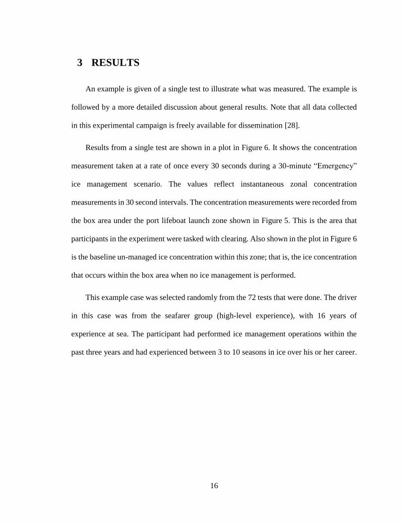
3 RESULTS

An example is given of a single test to illustrate what was measured. The example is

followed by a more detailed discussion about general results. Note that all data collected

in this experimental campaign is freely available for dissemination [28].

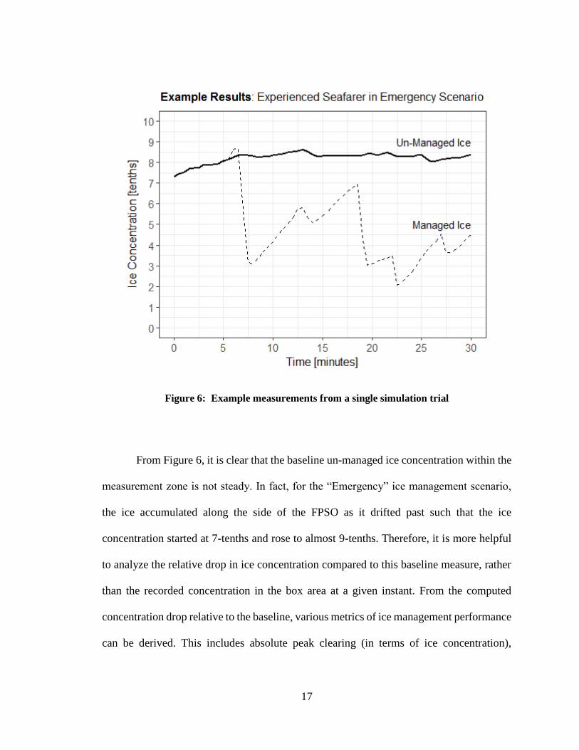
Results from a single test are shown in a plot in Figure 6. It shows the concentration

measurement taken at a rate of once every 30 seconds during a 30-minute “Emergency”

ice management scenario. The values reflect instantaneous zonal concentration

measurements in 30 second intervals. The concentration measurements were recorded from

the box area under the port lifeboat launch zone shown in Figure 5. This is the area that

participants in the experiment were tasked with clearing. Also shown in the plot in Figure 6

is the baseline un-managed ice concentration within this zone; that is, the ice concentration

that occurs within the box area when no ice management is performed.

This example case was selected randomly from the 72 tests that were done. The driver

in this case was from the seafarer group (high-level experience), with 16 years of

experience at sea. The participant had performed ice management operations within the

past three years and had experienced between 3 to 10 seasons in ice over his or her career.

17

Figure 6: Example measurements from a single simulation trial

From Figure 6, it is clear that the baseline un-managed ice concentration within the

measurement zone is not steady. In fact, for the “Emergency” ice management scenario,

the ice accumulated along the side of the FPSO as it drifted past such that the ice

concentration started at 7-tenths and rose to almost 9-tenths. Therefore, it is more helpful

to analyze the relative drop in ice concentration compared to this baseline measure, rather

than the recorded concentration in the box area at a given instant. From the computed

concentration drop relative to the baseline, various metrics of ice management performance

can be derived. This includes absolute peak clearing (in terms of ice concentration),

18

average clearing (in terms of ice concentration) and in total clearing (in km2 of ice cleared).

The reduction in ice concentration and the corresponding metrics are shown in Figure 7 for

the example case.

The ice concentration in the specified zones (Figures 4 and 5) was measured using

image post-processing of the Replay files recorded during simulation. Screen captures of

the Replay files were recorded at a rate of once every 30 seconds and the images were

subsequently processed using Matlab (Version 9.1.0 R2016b), where pixel counts of the

sequence of raster images were distinguished into three areas: open water, ice, and ship.

The concentration calculation (Equation 2.1) was computed as the total area of ice divided

by the area of the zone, corrected for the presence of the own-ship and FPSO, if and when

they entered the zone, by subtracting the ships’ water-plane areas from the calculation.

𝐼𝑐𝑒 𝐶𝑜𝑛𝑐𝑒𝑛𝑡𝑟𝑎𝑡𝑖𝑜𝑛 = ∑ 𝐴𝑟𝑒𝑎 𝑜𝑓 𝑖𝑐𝑒

𝐴𝑟𝑒𝑎 𝑜𝑓 𝑐𝑙𝑒𝑎𝑟𝑖𝑛𝑔 𝑧𝑜𝑛𝑒 Equation 3.1

19

Figure 7: The example case with three performance metrics illustrated

20

3.1 Average Clearing

Having examined a single case in Figures 6 and 7, we now look at the entire sample

of 36 participants tasked with two 30-minute scenarios each (72 total simulator trials and

36 hours of total simulator time) to characterize the data in terms of the chosen performance

metrics. Table 1 shows descriptive statistics for the average clearing metric for the cadet

(low-level experience) group for “Precautionary” and “Emergency” ice management

scenarios. Similarly, Table 2 shows descriptive statistics for the average clearing metric

for the seafarer (high-level experience) group for “Precautionary” and “Emergency” ice

management scenarios.

Table 1: Descriptive statistics for cadets’ average clearing (tenths concentration)

Scenario Concentration Mean

Standard

Deviation Minimum Median Maximum

Precautionary

IM

4 0.4 0.3 0.0 0.4 1.0

7 1.0 0.6 0.4 0.9 2.1

Emergency

IM

4 1.0 0.6 0.1 1.0 2.1

7 1.7 0.8 0.3 1.8 2.9

Table 2: Descriptive statistics for seafarers’ average clearing (tenths concentration)


Standard


Precautionary

IM

4 0.3 0.4 -0.1 0.2 1.0

7 1.2 0.7 0.2 1.0 2.5

Emergency

IM

4 1.6 0.5 0.8 1.7 2.1

7 2.6 0.7 0.9 2.9 3.4

21

From Tables 1 and 2, some characterizations can be made about the relative

performance of the two groups across like scenarios and concentration levels. For instance,

there is little difference between groups when comparing across the “Precautionary” ice

management scenario. The “Emergency” ice management scenario, on the other hand,

appears more suited to detect differences between groups for the average clearing metric.

Another important trend to note is that clearing is consistently higher at the higher

concentration level.

These trends are visually represented in the boxplots in Figure 8, which are grouped

by concentration and experience for all trials of the “Emergency” scenario.

Figure 8: Boxplots of average ice clearing for “Emergency” scenario

22

Half-normal plots of sub-plot effects and whole-plot effects are shown in Figures 9

and 10, respectively. Half-normal plots can be used to select significant factors for the

analysis. Here concentration (easy-to-change whole-plot factor) appears significant in the

sub-plot effects and experience (hard-to-change sub-plot factor) appears significant in the

whole-plot effects. The interaction effect is plotted on the whole-plot half-normal plot and

it does not appear significant, so it is dropped from the analysis. Restricted Maximum

Likelihood (REML) ANOVA (Table 3) is computed to formally test for significant effects.

It confirms that the experience and concentration factors are significant effects, with p-

values less than that prescribed by the acceptable Type 1 error rate of α = 5%.

The finding that concentration is significant is not surprising because the factor is

at least partly collinear with the response, average ice clearing. What is of interest is the

interaction effect occurring at different treatment combinations. Since the experience-

concentration interaction effect is not statistically significant we can reject the hypothesis

that ice management effectiveness increases with increasing experience and ice

concentration.

23

Figure 9: Half-normal plot of subplot effects

Figure 10: Half-normal plot of whole-plot

effects

Squares indicate positive effects; triangles indicate error estimates.

Note that when analyzing the results as if they came from a CRD using standard

ANOVA, the results yield the same conclusions. This is explained by the REML variance

component estimates (Table 3), which show a group variance of zero, indicating that the

whole-plot model is explaining all the variation between groups. The analysis is, in other

words, equivalent to a randomized design. Despite this, experimenters running similarly

designed experiments should take the same precaution and should not analyze results as if

they came from a CRD. This finding applies to all other metrics analyzed in this work

described in Section 3.2 to 3.5.

24

Table 3: REML ANOVA (average clearing)

Table 4: REML variance components table

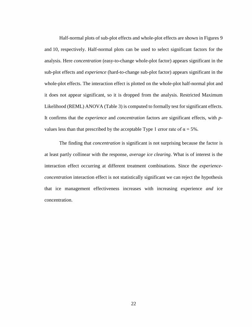
Key results of the model are shown in the effects plot in Figure 11. The plot shows

the average clearing metric for all 36 participant trials of the “Emergency” ice management

scenario. Data are summarized with Fisher’s Least Significant Difference (LSD) I-bars

around predictions at each treatment combination. This is an approximate way to check

whether predicted means at displayed factor combinations are significantly different. As

the slopes of the lines are almost parallel, it is clear there is no interaction effect between

the two factors on the average drop in managed ice concentration.

25

Figure 11: Interaction plot of concentration and experience on average clearing.

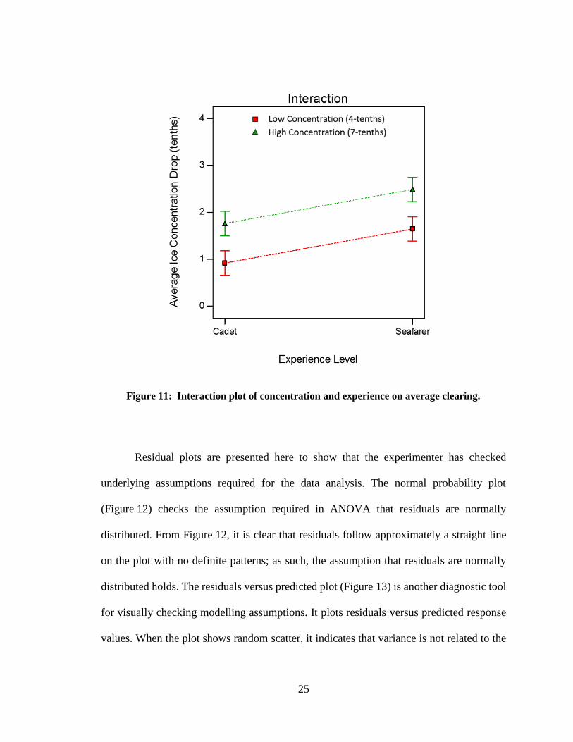
Residual plots are presented here to show that the experimenter has checked

underlying assumptions required for the data analysis. The normal probability plot

(Figure 12) checks the assumption required in ANOVA that residuals are normally

distributed. From Figure 12, it is clear that residuals follow approximately a straight line

on the plot with no definite patterns; as such, the assumption that residuals are normally

distributed holds. The residuals versus predicted plot (Figure 13) is another diagnostic tool

for visually checking modelling assumptions. It plots residuals versus predicted response

values. When the plot shows random scatter, it indicates that variance is not related to the

26

size of the response. This constant variance is called heteroscedasticity and is another

assumption required by ANOVA. It follows from Figure 13 that the assumption that

residuals are heteroscedastic is acceptable.

Figure 14 shows a plot of residuals versus run order. The random scatter indicates

that no time-related variables that went unaccounted for in the analysis are influencing

results. Finally, the Box-Cox plot in Figure 15 shows that based on a curve generated by

the natural logarithm of the sum of squares of the residuals, no power law transformation

is needed to stabilize variance or induce normality (transformation parameter lambda = 1).

The long vertical line in the Box-Cox plot indicates the best power transformation

parameter; the one currently used is represented by the short vertical line nearest to this

long line.

These important diagnostic checks are performed for all remaining analyses of

performance metrics in this work. Note that in the interest of abridging this work,

diagnostics plots are not shown for the remaining metrics in the text and are instead listed

in the Appendices (Section 7.2). The exception is Box-Cox plots, which are presented in

the text for models for which a power transformation was applied.

27

Figure 12: Normal plot of residuals

Figure 13: Residuals versus predicted

values

Figure 14: Residuals versus run order

Figure 15: Box-Cox plot for power

transform

28

3.2 Peak Clearing

Here we examine the entire sample of 36 participants tasked with 2 scenarios each

(72 total simulator trials) to characterize the data in terms of the peak ice clearing response,

measured in tenths concentration during 30-minute simulations. This metric is illustrated

in the example case in Figure 7. Table 5 shows descriptive statistics for the peak clearing

metric for the cadet (low-experience) group for “Precautionary” and “Emergency” ice

management scenarios. Table 6 shows the same statistics for the seafarer (high-experience)

group.

Table 5: Descriptive statistics for cadets’ peak clearing (tenths concentration)


Standard


Precautionary

IM

4 1.7 0.9 0.2 1.7 2.9

7 2.7 1.1 1.2 2.5 4.0

Emergency

IM

4 4.0 1.1 2.1 3.8 5.8

7 5.1 1.1 3.4 5.2 7.0

Table 6: Descriptive statistics for seafarers’ peak clearing (tenths concentration)


Standard


Precautionary

IM

4 1.3 0.9 0.2 1.0 3.1

7 2.9 1.3 1.2 3.2 5.0

Emergency

IM

4 4.2 1.0 2.8 4.0 5.8

7 5.6 1.1 2.9 5.9 7.0

29

From Tables 5 and 6, we may begin to characterize the relative performance of the

two groups across scenarios and across concentration levels. For instance, just as with the

average clearing metric, there is little difference between groups when comparing across

the “Precautionary” ice management scenarios. For the “Emergency” ice management

scenario there does appear to be some difference in performance, but not much. To

illustrate this point, the mean peak clearing in the “Emergency” scenario is 4.0 ± 1.1 for

the cadets; for the seafarers, it is 4.2 ± 1.0, just incrementally higher and less variable.

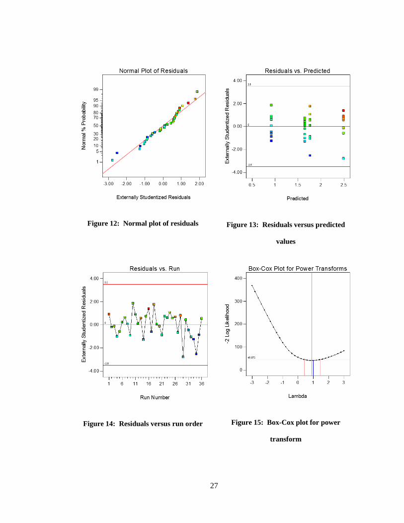
The boxplots in Figures 16 and 17 help to visualize the data. They are grouped by

concentration and experience for all trials of the “Precautionary” and “Emergency” ice

management scenarios, respectively.

30

Figure 16: Boxplots of peak ice clearing for “Precautionary” scenario

Figure 17: Boxplots of peak ice clearing for “Emergency” scenario

31

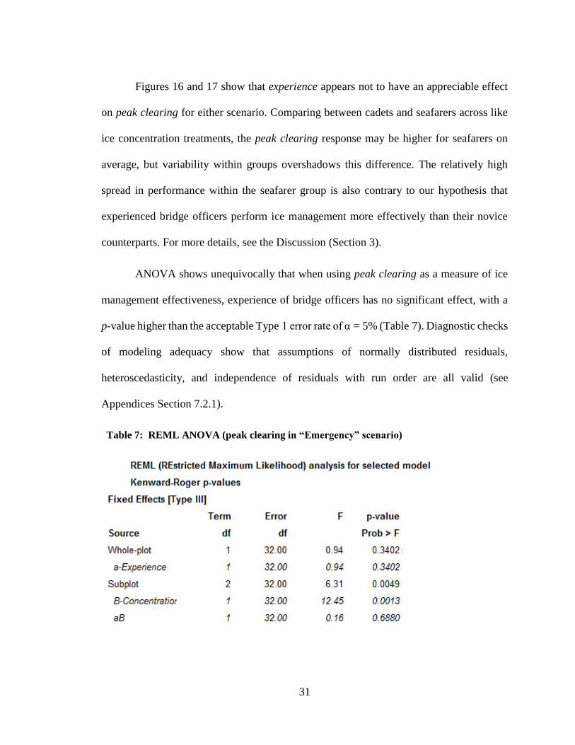
Figures 16 and 17 show that experience appears not to have an appreciable effect

on peak clearing for either scenario. Comparing between cadets and seafarers across like

ice concentration treatments, the peak clearing response may be higher for seafarers on

average, but variability within groups overshadows this difference. The relatively high

spread in performance within the seafarer group is also contrary to our hypothesis that

experienced bridge officers perform ice management more effectively than their novice

counterparts. For more details, see the Discussion (Section 3).

ANOVA shows unequivocally that when using peak clearing as a measure of ice

management effectiveness, experience of bridge officers has no significant effect, with a

p-value higher than the acceptable Type 1 error rate of α = 5% (Table 7). Diagnostic checks

of modeling adequacy show that assumptions of normally distributed residuals,

heteroscedasticity, and independence of residuals with run order are all valid (see

Appendices Section 7.2.1).

Table 7: REML ANOVA (peak clearing in “Emergency” scenario)

32

3.3 Total Clearing

The third performance metric in this study is total clearing, measured in square

kilometers of ice cleared from a defined area in 30 minutes. It is derived by summing the

incremental concentration drops (sampled at a rate of once every 30 seconds during the

simulation) over the 30-minute scenario duration, and then multiplying this total

concentration drop value by the area of the clearing zone. The derivation is expressed in

Equation 3.2. The clearing zone is outlined in Figure 5.

𝑇𝑜𝑡𝑎𝑙 𝐶𝑙𝑒𝑎𝑟𝑖𝑛𝑔 =1

2𝐴𝑧 ∑(𝐶𝑖 + 𝐶𝑖+1)∆𝑡

𝑛

𝑖=1

Equation 3.2

where 𝐴𝑧 = Zonal area

𝐶𝑖 = Incremental concentration drop

∆𝑡 = Sampling interval

Equation 3.2 may be generalized by a “swept” area as a function of ice drift speed,

as shown in Equations 3.3. This may be useful should experiments be repeated at a different

drift rate; however, the analysis presented will adopt the form expressed in Equation 3.2.

𝐴𝑧 = 𝑊𝑧𝑉𝑡𝑡𝑜𝑡 Equation 3.3

where 𝑊𝑧 = Zonal width

𝑉 = Ice drift rate

𝑡𝑡𝑜𝑡 = Total length of simulation time

33

Once again, we examine results of all 36 participants tasked with 2 scenarios each

(72 total simulator trials) to characterize the data in terms of the chosen performance

metric. Table 8 shows descriptive statistics for the total clearing metric for the cadet (low-

experience) group for “Precautionary” and “Emergency” ice management scenarios

separately. Table 9 shows the same statistics for the seafarer (high-experience) group.

Table 8: Descriptive statistics for cadets’ total clearing (km2)


Standard


Precautionary

IM

4 0.7 0.6 -0.1 0.6 1.6

7 1.6 0.9 0.7 1.4 3.4

Emergency

IM

4 0.4 0.3 0.05 0.4 0.9

7 0.8 0.4 0.1 0.8 1.3

Table 9: Descriptive statistics for seafarers’ total clearing (km2)


Standard


Precautionary

IM

4 0.6 0.7 -0.1 0.4 1.7

7 1.9 1.2 0.3 1.7 4.1

Emergency

IM

4 0.7 0.2 0.4 0.8 1.0

7 1.2 0.3 0.4 1.3 1.6

From Tables 8 and 9, just as with the average clearing and peak clearing metrics,

it is once again evident that little difference exists between groups when comparing across

the “Precautionary” ice management scenario. For the “Emergency” ice management

scenario, on the other hand, there does appear to be a notable performance difference.

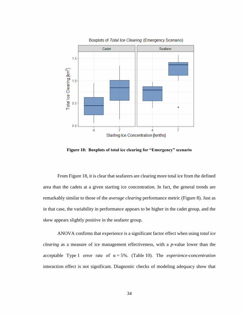
The boxplots in Figure 18 help to visualize this apparent trend. Data are grouped

by concentration and experience for all trials of the “Emergency” scenario.

34

Figure 18: Boxplots of total ice clearing for “Emergency” scenario

From Figure 18, it is clear that seafarers are clearing more total ice from the defined

area than the cadets at a given starting ice concentration. In fact, the general trends are

remarkably similar to those of the average clearing performance metric (Figure 8). Just as

in that case, the variability in performance appears to be higher in the cadet group, and the

skew appears slightly positive in the seafarer group.

ANOVA confirms that experience is a significant factor effect when using total ice

clearing as a measure of ice management effectiveness, with a p-value lower than the

acceptable Type 1 error rate of α = 5%. (Table 10). The experience-concentration

interaction effect is not significant. Diagnostic checks of modeling adequacy show that

35

assumptions of normally distributed residuals, heteroscedasticity, and independence of

residuals with run order are all valid (see Appendices Section 7.2.2).

Table 10: REML ANOVA (total clearing for “Emergency” scenario)


the total ice clearing metric for all 36 participant trials of the “Emergency” ice management

scenario. Data are summarized with Fisher’s LSD I-bars around predictions at each

treatment combination. This is an approximate way to check whether predicted means at

displayed factor combinations are significantly different. As the slopes of the lines are

almost parallel, it is visually clear there is no interaction effect between the two factors on

the average drop in managed ice concentration.

36

Figure 19: Interaction plot of concentration and experience on total ice clearing

37

3.4 Clearing-to-Distance Ratio

It was observed during simulation trials that seafarers accumulated a shorter trip

distance than cadets during the thirty minutes in which they were tasked with ice

management (Table 11). From the recorded observations, it should be noted that three

samples were lost from the seafarer group because of data logging errors during acquisition.

Because seafarers also cleared more ice on average and in total during the simulated

scenarios (Sections 2.1 and 2.3), it followed that effective ice management might have

been correlated with shorter trip distance. To explore this, we divided total ice clearing by

total trip distance to get a clearing-to-distance ratio for each 30-minute scenario, in units

of km2 of ice cleared per km travelled. The results of this new performance metric are

tabulated in a descriptive sense in Table 12 for cadets and Table 13 for seafarers.

Table 11: Total distance travelled (km)

Scenario Concentration n Mean

Standard

Deviation

Precautionary

IM

4 18 2.1 0.6

7 18 1.7 0.4

Emergency

IM

4 18 2.0 0.6

7 15 1.8 1.1

Table 12: Descriptive statistics for cadets’ clearing-to-distance ratio (km2/km)


Standard


Precautionary

IM

4 0.3 0.3 0.0 0.3 0.7

7 0.9 0.5 0.4 0.8 1.8

Emergency

IM

4 0.2 0.1 0.0 0.2 0.55

7 0.4 0.2 0.1 0.5 0.75

38

Table 13: Descriptive statistics for seafarers’ clearing-to-distance ratio (km2/km)


Standard


Precautionary

IM

4 0.4 0.5 -0.1 0.2 1.3

7 1.0 0.6 0.3 1.15 1.9

Emergency

IM

4 0.5 0.2 0.2 0.5 0.6

7 0.8 0.4 0.3 0.85 1.6

From Table 12 and Table 13, just as with all previous performance metrics, it is

once again evident that little appreciable difference exists between groups when comparing

across the “Precautionary” ice management scenario. For the “Emergency” ice

management scenario, on the other hand, there does appear to be a notable performance

difference.

From Tables 12 and 13, just as with all previous performance metrics, there is little

appreciable difference between groups when comparing across the “Precautionary” ice

management scenario. For the “Emergency” ice management scenario, on the other hand,

there does appear to be a notable performance difference.

The boxplots in Figure 20 help to visualize the data. They are grouped by

concentration and experience for all trials of the “Emergency” ice management scenario.

39

Figure 20: Boxplots of clearing-to-distance ratio for “Emergency” scenario

From Figure 20, it is clear that seafarers are clearing more total ice per distance

travelled from within the defined area compared to cadets at a given starting ice

concentration. The variability tends to be slightly higher in the seafarer group. This may be

an indication that a relatively large spread of expertise levels may exist within the

experienced seafarers, despite being better performers than the cadet group overall. More

on this subject is presented in the Discussion (Section 4).

ANOVA confirms that experience is a significant factor effect when using the

clearing-to-distance ratio as a metric of ice management effectiveness, with a p-value

lower than the acceptable Type 1 error rate of α = 5%. (Table 14). Also, the experience-

concentration interaction effect is not significant. Diagnostic checks of modeling adequacy

40

show that assumptions of normally distributed residuals, heteroscedasticity, and

independence of residuals with run order are all valid (see Appendices Section 7.2.3).

Table 14: REML ANOVA (clearing-to-distance ratio for “Emergency” scenario)


the clearing-to-distance ratio metric for all 36 participant trials of the “Emergency” ice

management scenario. Data are summarized with Fisher’s LSD I-bars around predictions

at each treatment combination.

41

Figure 21: Main effect plot of clearing-to-distance ratio versus experience

A square root power transformation was applied to stabilize variance and thereby

validate modelling assumptions (lambda = 0.5 in Box-Cox plot in Figure 22).

42

Figure 22: Box-Cox plot for power transform (clearing-to-distance ratio model)

43

3.5 Ice-Free Lifeboat Launch Time

During the “Emergency” scenario, each participant was told “to clear ice from

underneath the port lifeboat launch zone.” The lifeboat was visible near the port quarter of

the FPSO, and participants had remarked in exit interviews that this visual aid had helped

guide them to the location in which clearing was required. Although it was not the original

intention, it followed that the cumulative ice-free lifeboat launch time, measured in

minutes, would be a good metric of performance for this scenario.

To set up an appropriate analysis, the size and location of the lifeboat launch zone

had to be specified. The lifeboat drop zone radius was set at 8 m, based on the size required

to accommodate an 80-person capacity totally enclosed motor propelled survival craft

(TEMPSC) typical of those found on FPSOs. These lifeboats have dimensions of

approximately 10 m in length and 3.7 m in breadth. Results of experiments by Simões Ré

et al. (2002) found that a target drop point radius of approximately 1.5 m accommodated

launches for a TEMPSC from an offshore installation [29]. The 8 m “splash-zone” radius

which was set to circumscribe this target area would conservatively encompass offsets.

These offset distances might occur due to missed target points and setbacks by first wave

encounters. The origin of the zone was set at 8 m off the side of the port quarter of the

FPSO, so that the zone was tangent to the side of the FPSO hull. A schematic showing the

lifeboat launch zone is presented in Figure 23.

The cumulative time that the lifeboat splash zone was ice-free was computed using

Matlab image processing software. Successive replay files, captured at 30-second intervals

during simulation, were cropped to the shape and size of the lifeboat splash zone. From

44

here a pixel count of the raster image was computed; if the image had more colored pixels

than that of a cropped blank image, it meant that ice (or the own-ship itself in rare instances)

was in the lifeboat zone. For each successive ice-free image, a 30-second time increment

was added to the total time the zone was ice-free. The resulting total cumulative time was

therefore an approximation. Given that at a rate of current drift of 0.5 knots ice would drift

no more than 8 m in 30 seconds, coinciding with the radius of the lifeboat splash zone, this

approximate cumulative ice-free time estimate was considered appropriate for this study.

Figure 23: Port lifeboat launch zone (not to scale)

45

We can look at the sample of 36 participants tasked with the “Emergency” scenario

to characterize the data in terms the ice-free lifeboat launch zone performance metric. This

metric is measured in minutes of cumulative time that no ice is present in the 8 m radius

lifeboat launch zone. Table 15 shows descriptive statistics for the cumulative ice-free time

metric for the cadet (low-experience) group for the “Emergency” ice management scenario.

Table 16 shows the same statistics for the seafarer (high-experience) group.

Table 15: Descriptive statistics for cadets’ cumulative ice-free lifeboat launch times (minutes)


Standard


Emergency

IM

4 7.3 4.4 0.0 6.5 16.5

7 4.5 4.1 0.0 4.0 11.5

Table 16: Descriptive statistics for seafarers’ cumulative ice-free lifeboat launch times

(minutes)


Standard


Emergency

IM

4 10.0 3.2 7.0 8.5 16.5

7 11.6 7.0 0.0 13.0 19.0

From Tables 15 and 16 there is a clear difference between experience groups. The

mean cumulative time the lifeboat zone was ice free is consistently higher for the seafarers.

This trend is particularly striking at the high concentration treatment (7-tenths), in which

seafarers kept the lifeboat zone ice-free more than twice as long, on average, than cadets.

The boxplots in Figure 24 help to visualize the data. They are grouped by

concentration and experience for all trials of the “Emergency” ice management scenario.

46

Figure 24: Boxplots of cumulative ice-free lifeboat launch times during “Emergency”

scenario

From Figure 24 some additional characterizations can be made about the data. The

overall difference between groups in terms of cumulative ice-free lifeboat launch times is

significant. For example, the median values for the seafarer group at both concentration

treatments are higher than even the respective third quartiles recorded for the cadet group.

The spread is lower for the seafarers in the low concentration treatment (4-tenth), but higher

in the high-concentration treatment (7-tenths). Despite the better performance overall, the

high spread may indicate a relative higher degree of expertise variability within the seafarer

group. This is a similar trend observed as when using total ice clearing to measure

performance. Also, it is remarkable that responses are higher for the 7-tenths treatment in

47

the seafarer group. The response in this case is independent of starting ice concentration

and the high-level treatment (7-tenths) was expected to represent a significant challenge

compared to the low treatment (level 4-tenths). This surprising result cannot be explained

by experience difference within the seafarer group, either, as experience level for both

treatments were similar (4-tenths treatment: seafarers’ average years at sea = 20 ± 9;

7-tenths treatment: seafarers’ average years at sea = 20 ± 10).

ANOVA shows that experience is a significant factor on the cumulative ice-free

lifeboat launch time, with a p-value higher than that prescribed by the acceptable Type 1

error rate of α = 5%. (Table 17).

Table 17: REML ANOVA (cumulative ice-free lifeboat launch time)


the cumulative ice-free time metric for all 36 participant trials of the “Emergency” ice

management scenario. Data are summarized with Fisher’s LSD I-bars around predictions

at each treatment combination.

48

Figure 25: Main effect plot of cumulative ice-free lifeboat launch time versus experience

Diagnostic checks of modeling adequacy show that assumptions of normally

distributed residuals, heteroscedasticity, and independence of residuals with run order are

all valid. A square root power transformation was applied to stabilize variance and thereby

validate modeling assumptions (lambda = 0.5 in Box-Cox plot in Figure 26).

49

Figure 26: Box-Cox plot for power transform (cumulative ice-free lifeboat launch time

model)

50

3.6 Ice Management Tactics

So far, considerable effort has gone into showing that a statistically significant

difference exists between experienced seafarers and inexperienced cadets when it comes

to performance in ice management. To measure performance in ice management, we used

five different metrics of overall effectiveness: average clearing, peak clearing, total

clearing, distance-to-clearing ratio, and cumulative ice-free lifeboat launch time.

Differences were detected between groups only when making assessments with the

“Emergency” scenario. The “Precautionary” scenario (Figure 4) failed to detect any

differences between experience groups. Suggestions as to why this may be the case are

presented in the Discussion (Section 3). For the “Emergency” scenario, with the exception

of peak clearing, each metric showed that experience had a significant influence on ice

management effectiveness. These findings underscore an important question: what is the

seafarer group doing that makes them more effective than the cadets? We examine this

question in this section.

As a starting point, we may begin to understand what effective ice management looks

like by plotting the tracks taken by seafarers during the 30-minute simulation. Additionally,

if we trace all the tracks taken by seafarers in one plot, and then repeat this for cadets’

tracks, we should begin to see spatial differences in maneuvers that may characterize

underlying differences in tactics. The problem is, if we do this we end up with messy plots

from which it is difficult to ascertain meaningful results. One solution is to present

“heatmaps” of the respective groups’ tracks (Figures 27 and 28). The heatmaps are

constructed by dividing the simulation area into bins and counting instances in which the

51

own-ship passes through a given bin during simulations. The aggregate counts for a given

scenario are assigned colors: the higher the number, the brighter the corresponding color

for that bin. This way we have a clearer way of visualizing the two groups’ aggregate

tracks. Figures 27 and 28 display such tracks for the high-level (7-tenths) concentration

cases for the “Emergency” scenario for cadets and seafarers, respectively. Similar plots can

be constructed for the low-level (4-tenths) concentration cases, although they are not

included here because the differences between experience levels is most pronounced in the

7-tenths concentration level.

Figure 27: Heatmap for cadets’ tracks

during “Emergency” scenario

Figure 28: Heatmap for seafarers’ tracks

during “Emergency” scenario

From Figures 27 and 28 it is obvious that spatial differences exist between the cadet

group and the seafarer group. For one, seafarers appear to focus their position on a single

52

area (visible as the only bright patch in the heatmap in Figure 28), whereas cadets are

divided into two or three relatively large areas (Figure 27). From this insight, the seafarers’

chosen maneuvering tactics may be characterized as more uniformly executed. Because

participants were actively discouraged from discussing the experiment with others, each

trial was independently orchestrated. And yet, there appears to be a high degree of

similarity among seafarers’ chosen tactics. Specifically, they appear to focus just upstream

of the port lifeboat launch zone. The position tactic proved to be effective, as evidenced by

results of the clearing-to-distance ratio metric (Section 2.4), which detected a distinct

difference between experience groups in how much ice was cleared per kilometer travelled.

From boxplots of cumulative ice-free lifeboat launch time (Figure 24) there was

considerable variability in seafarer performance. This same trend is visible for other

metrics (Figures 8, 18, and 20). So, despite seafarers performing more effectively than

cadets on average, it merits a closer examination within the seafarer group to determine

what may distinguish an individual’s effective trial compared to another individual’s

ineffective one. Figure 29 plots two tracks based on the midships position of the own-ship

during the 30-minute simulations scenario. The two tracks represent the best and the worst

of all seafarers, where best and worst are measured by corresponding highest and lowest

amounts cumulative ice-free lifeboat launch time, respectively. The resulting difference

represents the largest single gap in performance between any two individuals for this

scenario, including cadets. Clearly, positioning makes a difference, and the “best” track in

this case demonstrates a highly effective tactic. The track shows a straightforward line

heading toward the lifeboat launch zone, where it stops upstream, swings about to create a

53

lee down-drift of its port side and holds position for the duration of the simulated scenario.

The “worst” track, on the other hand, plots a track farther upstream of the FPSO and

lifeboat launch zone, covering almost twice as much as distance as the “best” track.

An inspection of the Replay files provides further clues as to what may distinguish

successful tactics. Figures 30 and 31 show that heading with respect to the ice also plays a

major role. For instance, the best trial (Figure 30) shows that a “wedging” maneuver (so-

called by the seafarer who produced it), whereby the vessel’s quarter is positioned close to

the FPSO and its heading is approximately 30 degrees off the FPSO heading, effectively

traps the ice between the two vessels. Ice accumulated and eventually drifted around the

wedge created by the stand-by vessel, effectively clearing the area downstream that

required attention. The worst trial (Figure 31) appears to show an attempt to clear ice

sideways, using the side thrusters to clear ice while maneuvering upstream. The issue with

this appears to be that ice drifting into the bow of the FPSO was deflected along the length

of the port side by the current. From here the ice subsequently drifted into the lifeboat

launch zone, unimpeded by the vessel’s presence. Moreover, during the best trial

(Figure 30), use of the aft console allowed good visibility of the deck, which would have

been an advantage while working close to the FPSO. For the worst trial, on the other hand,

the stand-by vessel was oriented bow-on to the FPSO, and visibility over the bow would

have been limited. Much of the ice between the bow and the FPSO would have been

completely hidden from view. Inspection of the Replay files can therefore provide valuable

insights into good practices in ice management to complement plots of tracks, which show

a more general picture of overall tactics.

54

Figure 29: Plot of best and worst tracks for “Emergency” scenario.

Criterion is cumulative ice-free lifeboat launch time.

Figure 30: Midway mark (15 min) during

“Emergency” scenario for best trial

Figure 31: Midway mark (15 min) during

“Emergency” scenario for worst trial

55

Exit interviews were conducted for all participants and these may also offer

important clues about the tactics. For example, the “best” track from Figure 29 (depicted

in the Replay images in Figure 30) was performed by a seafarer code-named C79, who was

asked during the after-action interview to reflect on the tactics undertaken during the

simulation scenario. C79 was a master with approximately 30 years of experience at sea,

which included more than 10 seasons of operations in sea ice (including ice management),

most recently within the past 3 years. Note than identifying details are not provided to

respect participants’ anonymity. Asked about the strategy employed in the simulation

scenario, C79 stated:

I caught a large floe, which is advantageous to push against. My stern thrusters

were at 100% [power allocation], pushing against trapped ice. I used side thrusters

to maintain position. I tried to maintain a 30-degree heading using my thrusters.

Ice travelling down would drift down and around [my bow]. I moved fast at the

start to take advantage of clear water. Then I slowed in ice to less than 3 knots.

Compared to the Replay file imagery and the plots of tracks before that, exit

interview transcripts such as this provide valuable qualitative information about ice

management tactics. For example, we now know that a large ice floe was used strategically

to block others, and that the ice trapped in the “wedge” was almost overpowering the own-

ship. Additionally, when asked about what factors might be important for success in such

a scenario, C79 replied, “[One should] get set up instead of moving too much.” The track

56

plot (Figure 29), which showed a direct path to a location upstream of the lifeboat launch

zone and minimal movement thereafter, corroborates this assertion, as does the quantitative

metric clearing-to-distance ratio (Section 2.4), which showed that ice clearing and distance

travelled were inversely correlated (and for which C79 was the peak performer).

In comparison, the “worst” track was performed by a master, code-named S41, who

had accumulated 10 years of experience. This included 3 to 10 seasons of operations in sea

ice (including ice management), most recently within the past 3 years.

When asked about tactics employed for the “Emergency” scenario, S41 stated that

he or she had been attempting to implement an industry procedure. Details about which

procedure this referred to were not provided. When asked about what changes might be

done in a hypothetical repeat trial of the simulated scenario, S41 stated:

[In a repeat I would] come up closer to the bow of the FPSO. I would’ve cleaned

out ice closer [to the FPSO], stern-first.

Interestingly, S41’s remarks about positioning closer to the FPSO and maneuvering

stern-first are both characteristics observed during C79’s successful maneuver. This

suggests that had S41 had the chance to repeat the trial, he or she would have applied a

tactic similar to that of C79. Although learning effects were not directly measured in this

experiment, this is a strong qualitative indicator that learning effects may exist for ice

management simulator training.

57

4 DISCUSSION AND FUTURE WORK

The experimental campaign undertaken highlights the importance of appropriate

simulation scenario design when assessing ice management effectiveness in a marine

simulator. The “Precautionary” scenario (Figure 4) failed to detect any significant

difference between the two experience groups, whereas the “Emergency” scenario did. In

the former, individuals were tasked with keeping the port and starboard lanes of the FPSO

clear of ice as a precautionary measure so that lifeboats would be able to launch safely in

the event of a major event. Why did this scenario fail to detect differences between

experience groups? The question may be best answered by the experienced seafarers who

performed it. Transcripts of exit interviews taken shortly after simulation showed that out

of 18 seafarers, 7 said that “clearing of both sides was not possible with a single vessel”,

with 5 of these 7 specifying that “two vessels are required for such a scenario.”

Furthermore, 2 individuals stated that they had performed a similar precautionary ice

management exercise “in real life,” and in those cases at least two stand-by vessels had

been on-site to complete the job. It follows that the scenario would have been better suited

for two or more stand-by vessels working together, rather than just the one own-ship. In

other words, the “Precautionary” scenario was challenging by virtue of having a single

vessel attempting a multi-vessel mission. This challenge overshadowed differences in

performance that could be explained by differences in officer experience. This serves to

illustrate an important design element for experimenters and simulator course developers:

care and attention must go into developing an appropriate scenario if one hopes to measure

an effect.

58

Care must also be taken when applying performance metrics to simulation scenarios. In

this study, when using a specified region in which to measure pack ice modification, global

measures of average and total ice clearing indicated significant differences between

experience groups, whereas the event-specific peak ice clearing indicated no differences at

all. This finding may help model course developers and experimenters select appropriate

performance metrics for similar applications. Moreover, for the clearing-to-distance ratio

and cumulative ice-free lifeboat launch time performance metrics, only experience was

found to be a significant factor on effectiveness response. This meant that effectiveness

was independent of starting ice concentration for these two metrics, making them ideal

candidates for measuring performance in simulation scenarios.

There were some important limitations with the simulator that must be noted. Most

importantly, this included the inherent difficulties associated with judging spatial distance

from a two-dimensional screen. With no radar present, either, the officers had to rely on

the VHF radio for information about distances to specified targets. The officers’ watch-

keeper (role-played by an experimenter at the Instructor Station) would report back

distances measured from a built-in software tool, when asked. Another limitation of the

simulator stemmed from the omission of transverse and astern velocities on the display

screen in the bridge console. Only total speed and heading were displayed. During ice

management close to the FPSO, subtle shifts in speed in any direction were important for

the officer to know about as he or she adjusted controls to maintain good position. Finally,

visibility from the simulator bridge console was an issue. In a real ship, officers can walk

to the wing and look out along the side of the vessel to see ice. This probably made ice

59

management in the simulator more challenging since ice was effectively invisible off the

bow and sides of the own-ship. Improvements could perhaps be made to the simulator

technology and the resulting data collected would likely be more reliable. Regardless, the

simulator used in the experiment met the intended scope of the research: it was sufficiently

representative to detect differences between bridge officer experience groups and it was

able to characterize general principles of good ice management practices.

So far, it has not been mentioned whether the seafarers had had formal training in

ice prior to completing the test trial. This information was collected in experience

questionnaires and it was found that out of the 18 experienced seafarers tested, only 6

reported to have had formal training in ice management, with 4 of these describing their

training as “Basic” and the remaining 2 describing it as “Advanced.” Despite this, 17 out

of 18 reported to have done ice management in the field. The lack of formal training in ice

may explain the high degree of variability generally observed in performance measured

within the seafarer group (Figures 8, 18, 20, and 24).

It was also observed during exit interviews that 5 out of 12 seafarers operating

OSVs and AHTS vessels stated that they were accustomed to dynamic positioning (DP)

for station keeping and maneuvering, which is the industry norm for vessels of these types.

However, from the exit interview it was clear that few, if any, officers would rely on DP

for station keeping in drifting pack ice. Apparently, this was due to the nature of loading

that sea ice imposes on the hull. With this in mind, the experiments may be viewed as

scenarios presenting conditions that required manual take-over of positioning controls.

Bainbridge (1983) argues that the skills required for manual take-over from an autonomous

60

control system like DP need special attention and training if they are to be accomplished

with success [30]. In our experiments, only a third of operators had formal training in this

area despite all but one having completed it in the field, potentially highlighting a gap in

training for manual take-over of vessel position and station keeping in drifting pack ice.

Learning effects, which are observed when a scenario is repeated with improved

results, are often of interest in simulator experiments. Learning effects were not directly

measured in this experiment because repeat trials were not conducted. Still, they were

indirectly detected from the interviews. Specifically, we compared the individuals’

performance as-measured in the “Emergency” scenario to corresponding performance

scores as-reported in a self-assessment during exit interviews. The self-reported score was

on a subjective scale of 1 to 5, where 1 was poor and 5 was excellent. For the measured

performance, the cumulative ice-free lifeboat launch times for each trial were scaled

linearly from 1 to 5 so that 1 equated to 0 minutes and 5 equated to approximately 18

minutes (95th percentile of recorded cumulative times). Note that because the 95th

percentile was used, some “actual” scores were above 5. The results were plotted and a

locally weighted scatterplot smoothing (LOESS) fit (weight parameter = 0.75) was used to

explore trends (Figure 32). The LOESS fit matched very closely to the unity line, indicating

that on average, participants were strikingly accurate when perceiving the effectiveness of

their own performance. A closer look, though, reveals this trend is only slightly linear

(Pearson’s ρ = 0.56, p = 0.0003), indicating that this perception is only accurate on average

for a relatively large group size and that variation is quite high. Still, this finding indicates

61

that on average, individuals may accurately recognize their own needs for training after

having completed a simulation scenario.

Figure 32: Plot of actual versus self-reported performance scores with LOESS line

62

5 CONCLUSIONS

Experienced crew have been shown to perform ice management more effectively than

inexperienced crew in a simulator experiment. Based on the results, it can be concluded

that experience level of bridge officers onboard a vessel tasked with an ice management

operation will significantly influence the resulting effectiveness. Effectiveness was

measured in four ways: i) average ice clearing in a defined area (tenths concentration),

ii) total ice clearing in a defined area (km2), iii) clearing-to-distance ratio (km2/km), and

iv) cumulative ice-free lifeboat launch time (in minutes). The latter of the four metrics

applied to the “Emergency” scenario, only.

The hypothesis that the human factor of expertise influences effectiveness of ice

management operations has been formally tested and accepted in this experimental

campaign. Also, the hypothesis that the human factor of experience level has a larger effect

when combined with higher concentration (positive interaction effect) has been formally

tested and rejected.

The question about what made experienced seafarers more effective than

inexperienced cadets was addressed using a combination of quantitative and qualitative

data. The data came from three sources: i) plots of position during simulation,

ii) screenshots captured from Replay files, and iii) exit interviews. This information

allowed us to characterize good ice management practices in terms of a chosen

performance metric for our simulated scenario.

63

Overall, the results provide a basis for assessing what the experienced crew does that

the inexperienced crew does not in terms of operating tactics. This could offer insights for

informing good practices in ice management as they apply to offshore operations. The gap

between the two groups, as well as the variability within the respective groups, also

provides a quantitative basis for the design of a training curriculum that could close the

performance gap and reduce its variability.

64

6 REFERENCES

[1] R. Haimelin, F. Goerlandt, P. Kujala and B. Veitch, "Implications of novel risk

perspectives for ice management operations," Cold Regions Science and Technology,

vol. 133, pp. 82-93, 2017.

[2] K. Eik, "Review of experiences with ice and iceberg management," Journal of

Navigation, vol. 61, pp. 557-572, 2008.

[3] A. Keinonen, M. Shirley, G. Liljeström and R. Pilkington, "Transit and stationary

coring operations in the central Polar pack," in Icetech’06 Conference, Society of

Naval Architects and Marine Engineers, Banff, 2006.

[4] A. Keinonen, R. Browne, E. Lam and W. Jolles, "Six Years in Sakhalin Offshore

Oil–Management of Risk for Operations In Ice," in Icetech’06 Conference, Society

of Naval Architects and Marine Engineers, Banff, 2006.

[5] B. Maddock, A. Bush, T. Wojahn, T. Kokkinis, A. Younan and Hawkins, "Advances

in ice management for deepwater drilling in the Beaufort sea," in Proceedings, Port

and Ocean Engineering under Arctic Conditions, Montréal, 2011.

[6] A. Barker, G. Timco, M. Sayed and B. Wright, "Numerical simulation of the Kulluk

in pack ice conditions," in Proceedings, Symposium on Ice, Gdansk, 2000.

[7] D. Spencer and W. Molyneux, "Predicting pack ice loads on moored vessels," in

Proceedings, Ship and Offshore Technology, Busan, 2009.

65

[8] J. Hamilton, C. Holub and J. Blunt, "Simulation of ice management fleet operations

using two decades of Beaufort Sea ice drift and thickness time histories," in

Proceedings, Offshore and Polar Engineering Conference, Maui, 2011.

[9] K. Eik and O. Gudmestad, "Iceberg management and impact on design of offshore

structures," Cold Regions Science and Technology, vol. 63, pp. 15-28, 2010.

[10] L. Zhou, B. Su, K. Riska and T. Moan, "Numerical simulation of moored structure

station keeping in level ice," Cold Regions Science and Technology, vol. 71, pp. 54-

66, 2011.

[11] P. Dunderdale and B. Wright, "Pack Ice Management on the Southern Grand Banks

Offshore Newfoundland," National Research Council of Canada, 2005.

[12] NVIDIA Corporation, PhysX Version 2.8.1, Santa Clara, 2008.

[13] R. Lubbad and S. Løset, "A numerical model for real-time simulation of ship–ice

interaction," Cold Regions Science and Technology, vol. 65, no. 2, pp. 111-127,

February 2011.

[14] N. Dahlstrom, S. Dekker, R. van Winsen and J. Nyce, "Fidelity and validity of

simulator training," Theoretical Issues in Ergonomics Science, vol. 10, no. 4, pp. 305-

314, 2009.

66

[15] R. Hanzu-Pazara, P. Arsenie and L. Hanzu-Pazara, "Higher performance in maritime

education through better trained lecturers," TransNav: International Journal on

Marine Navigation and Safety of Sea Transportation, vol. 4, no. 1, pp. 87-93, 2010.

[16] M. Hontvedt, "Simulations in Maritime Training: A video study of the socio-

technical organisation of ship simulator training," University of Oslo, Oslo, 2014.

[17] M. Hontvedt, "Professional vision in simulated environments — Examining

professional maritime pilots' performance of work tasks in a full-mission ship

simulator," Learning, Culture and Social Interaction, vol. 7, pp. 71-84, 2015.

[18] C. Sellberg, "Simulators in bridge operations training and assessment: a systematic

review and qualitative synthesis," WMU Journal of Maritime Affairs, vol. 16, no. 2,

pp. 247-263, 2017.

[19] C. Sellberg, O. Lindmark and H. Rystedt, "Learning to navigate: the centrality of

instructions and assessments for developing students’ professional competencies in

simulator-based training," WMU Journal of Maritime Affairs, pp. 1-17, 2018.

[20] R. S. Kennedy, N. E. Lane, K. S. Berebaum and M. G. Lilienthal, "Simulator sickness

questionnaire: an enhanced method for quantifying simulator sickness," International

Journal of Aviation Psychology, vol. 3, no. 3, pp. 203-220, 1993.

[21] D. Montgomery, "1.3 Basic Principles," in Design and Analysis of Experiments (8th

Edition), John Wiley & Sons, 2013.

67

[22] J. Cohen, Statistical power analysis for the behavioral sciences, Ney York: Academic

Press, 1998.

[23] S. Kowalski and K. J. Potcner, "How to recognize a split-plot experiment," Quality

Progress, vol. 36, no. 11, pp. 60-66, 2003.

[24] B. Jones and C. Nachtsheim, "Split-plot designs: what, why, and how," Journal of

Quality Technology, vol. 41, no. 4, pp. 340-361, 2009.

[25] C. Daniel, "Use of half-normal plots in interpreting factorial two-level experiments,"

Technometrics, vol. 1, no. 4, pp. 311-341, 1959.

[26] K. Potcner and S. Kowalksi, "How To Analyze A Split-Plot Experiment," Quality

Progress, vol. 37, no. 12, pp. 67-74, 2004.

[27] D. Montgomery, "3.4 Model Adequacy Checking," in Design and Analysis of

Experiments (8th Edition), John Wiley & Sons, 2013.

[28] E. Veitch, "Influence of Bridge Officer Experience on Ice Management Effectiveness

(OERC2018-011)," Memorial University of Newfoundland, Ocean Engineering

Research Centre, St. John's, 2018.

[29] A. Simões Ré, B. Veitch and D. Pelley, "Systematic investigation of lifeboat

evacuation performance," Transactions, Society of Naval Architects and Marine

Engineers, vol. 110, 2002.

68

[30] L. Bainbridge, "Ironies of automation," IFAC Proceedings, vol. 15, no. 6, pp. 129-

135, 1982.

[31] J. H. Zar, Biostatistical Analysis, Upper Saddle River, N.J.: Prentice-Hall, 1996.

69

7 APPENDICES

7.1 Power Analysis and Experiment Sizing

A common question that arises in experimental design is how many samples is

enough? The question suggests that there is an optimal number of samples: one that meets

the needs of the experiment by detecting the effect under investigation with sufficient

accuracy, but one that does not exceed that number and that does not waste valuable time

and resources in doing so [22], [31]. An estimate for the minimum sample size required for

this experiment was produced using a prospective power analysis.

A prospective power analysis means that the experiment is sized based on a defined

statistical power level and based on an estimate of the spread, or standard deviation, of the

response being analyzed. As a first step, it is important that the objective of the experiment

be defined. For illustrative purposes, we may define the objective as follows: the goal of

the experiment is to compare cumulative ice-free lifeboat launch times during a 30-minute-

long ice management simulation between low- and high-experience groups. Such a

comparison suggests a comparison test between means, like the basic 2-sample t-test. As

such, we can produce an estimate of the minimum sample size required for our experiment

based on a power analysis of 2-sample t-test using this response variable. Note that this

will produce an estimate only (effect estimates of the actual results were computed more

precisely using REML ANOVA techniques in Section 3). The results of prospective power

analyses such as the one shown here will therefore not be exact; however, given that it is a

tool meant to inform sizing given the best available information prior to running the

70

experiment, such a methodology is suitable for this application. The procedure also relies

upon the assumption that response data will be normally distributed and that each group

will have the same distribution. These are strong assumptions and are especially so given

the lack of prior data; as such, it is highlighted once again that power analyses should be

used as a guide only and not as an explicit method for determining minimum sample size.

The method and results shown here were produced in Minitab (Version 18.1). Curves

of statistical power for the experiment were computed given the standard deviation of the

response and any two of the three following items: i) sample size, ii) difference in means

(effect size), or iii) power values. Because we wished to obtain curves for sample size, the

latter two of the three will be defined over a range of possible differences in means that we

might expect. This is computed at an acceptable Type 1 error rate of α = 0.05, as shown in

the summary of inputs in Table 18.

Table 18: Inputs for prospective power analysis based on 2-sample t-test

Range of expected differences in means: 2, 3, 4, 5, 6, 7, and 8 minutes

Power value: 0.8 or 80%

Estimated standard deviation of the response: 4 minutes

Acceptable alpha risk (Type 1 error rate) α = 0.05 or 5%

Ideally, an estimate of the standard deviation for the response variable would be

obtained either from the literature, from prior experiments, or from a meta-analysis. The

unique nature of the experiment in this study, though, precludes such a strategy because no

71

similar work has been done before. A pilot study could have been done, however for this

experiment it was not considered feasible given the difficulty in obtaining human

participants. A reasonable best estimate, therefore, based on good judgment and expert

advice was considered an appropriate substitute. Correspondingly, an effect size estimate

(for the response cumulative ice-free lifeboat launch time measured across experience

groups) of 4 minutes was proposed, with an expected mean difference between groups

centered on approximately 5 minutes. The null hypothesis assumed equivalency between

groups and the alternative hypothesis was that the low-experience group had a lower

response. A power of 80% was considered acceptable for this design and the alpha risk, or

Type 1 error rate, was set to 0.05 or 5%. The results of the power analysis with these inputs

are summarized in Table 19.

Table 19: Results of prospective power analysis for 2-sample t-test

Difference Sample Size Target Power Actual Power

2 51 0.8 0.8059

3 23 0.8 0.8049

4 14 0.8 0.8241

5 9 0.8 0.8138

6 7 0.8 0.8409

7 5 0.8 0.8100

8 4 0.8 0.8015

From Table 19 a sample size between n = 14 and n = 23 would be appropriate for

detecting differences in means of cumulative ice-free lifeboat launch times between groups

72

of 4 and 3 minutes. This was based on the inputs listed in Table 18. Note that the sample

sizes indicated in Table 19 are for each group.

The actual sample size n used in the experiment for each experience group was n = 18

(there were two experience groups – a low and a high – so there were n = 36 samples in

total). Having selected this sample size, the power analysis method could be repeated, this

time to determine the minimum detectable difference in means, or effect size, between

groups given the sample size and power value used. A power curve is produced in

Figure 33 that shows an intersection (represented with a dot) at 80% power corresponding

to a minimum detectable effect size of approximately 3.38.

Figure 33: Prospective power curve for 2-sample t-test

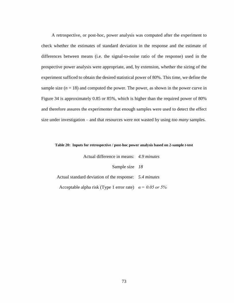
73

A retrospective, or post-hoc, power analysis was computed after the experiment to

check whether the estimates of standard deviation in the response and the estimate of

differences between means (i.e. the signal-to-noise ratio of the response) used in the

prospective power analysis were appropriate, and, by extension, whether the sizing of the

experiment sufficed to obtain the desired statistical power of 80%. This time, we define the

sample size (n = 18) and computed the power. The power, as shown in the power curve in

Figure 34 is approximately 0.85 or 85%, which is higher than the required power of 80%

and therefore assures the experimenter that enough samples were used to detect the effect

size under investigation – and that resources were not wasted by using too many samples.

Table 20: Inputs for retrospective / post-hoc power analysis based on 2-sample t-test

Actual difference in means: 4.9 minutes

Sample size 18

Actual standard deviation of the response: 5.4 minutes

Acceptable alpha risk (Type 1 error rate) α = 0.05 or 5%

74

Figure 34: Retrospective / post-hoc power curve for 2-sample t-test

75

7.2 Diagnostics Plots

The following section present diagnostics plots of residual error and Box-Cox plots

for power transformations for each of the separate analyses described in Sections 3.2 to

3.5, respectively (peak clearing, total clearing, clearing-to-distance ratio, and ice-free

lifeboat launch time metrics). All modelling diagnostics apply to the “Emergency” ice

management scenarios results analyzed and presented in the text.

7.2.1 Diagnostics Plots for Peak Clearing Metric

Figure 35: Normal plot of residuals (peak

clearing)


values (peak clearing)

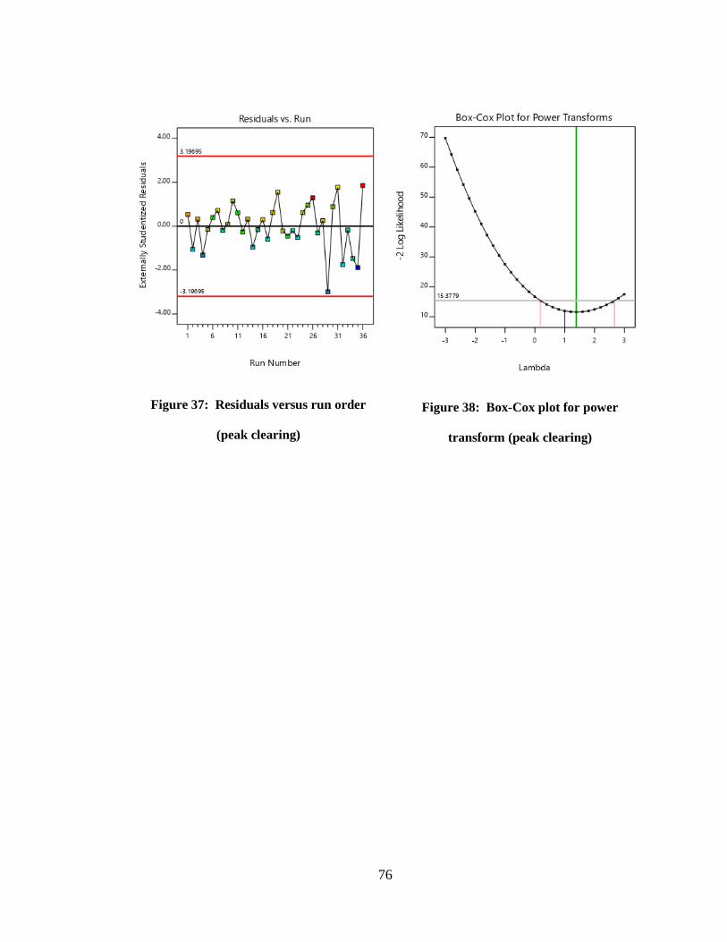
76


(peak clearing)


transform (peak clearing)

77

7.2.2 Diagnostics Plots for Total Clearing Metric

Figure 39: Normal plot of residuals (total

clearing)

Figure 40: Residuals versus predicted values

(total clearing)

Figure 41: Residuals versus run order (total

clearing)


transform (total clearing)

78

7.2.3 Diagnostic Plots for Clearing-to-Distance Ratio Metric

Figure 43: Normal plot of residuals

(clearing-to-distance ratio)


values (clearing-to-distance ratio)


(clearing-to-distance ratio)


transform (clearing-to-distance ratio)

79

7.2.4 Diagnostic Plots for Ice-Free Lifeboat Launch Time Metric

Figure 47: Normal plot of residuals (ice-free

lifeboat launch time)


values (ice-free lifeboat launch time)

Figure 49: Residuals versus run order (ice-

free lifeboat launch time)


transform (ice-free lifeboat launch time)

master of engineering ocean & naval architectural

Documents