mass2, modular aquatic simulation system in two … · 2007-11-10 · pnnl-14820-2 mass2 modular...
TRANSCRIPT

PNNL-14820-2
MASS2
Modular Aquatic Simulation System in
Two Dimensions
User Guide and Reference
W. A. Perkins
M. C. Richmond
September 2004
Prepared for the U.S. Department of Energy
under Contract DE-AC06-76RL01830

DISCLAIMER
United States Government. Neither the United States Government nor any agency
thereof, nor Battelle Memorial Institute, nor any of their employees, makes any
warranty, express or implied, or assumes any legal liability or responsibility
for the accuracy, completeness, or usefulness of any information, apparatus,
product, or process disclosed, or represents that its use would not infringe
privately owned rights. Reference herein to any specific commercial product,
process, or service by trade name, trademark, manufacturer, or otherwise does
not necessarily constitute or imply its endorsement, recommendation, or favoring
by the United States Government or any agency thereof, or Battelle Memorial
Institute. The views and opinions of authors expressed herein do not necessarily
state or reflect those of the United States Government or any agency thereof.
PACIFIC NORTHWEST NATIONAL LABORATORY
operated by
BATTELLE
for the
UNITED STATES DEPARTMENT OF ENERGY
under Contract DE-AC06-76RLO1830
Printed in the United States of America
Available to DOE and DOE contractors from the
Office of Scientific and Technical Information,
P.O. Box 62, Oak Ridge, TN 37831-0062;
ph: (865) 576-8401
fax: (865) 576-5728
email: [email protected]
Available to the public from the National Technical Information Service,
U.S. Department of Commerce, 5285 Port Royal Rd., Springfield, VA 22161
ph: (800) 553-6847
fax: (703) 605-6900
email: [email protected]
online ordering: http://www.ntis.gov/ordering.htm
This document was printed on recycled paper.
(8/00)

PNNL-14820-2
MASS2
Modular Aquatic Simulation System in Two
Dimensions
User Guide and Reference
W. A. Perkins
M. C. Richmond
September 2004
Prepared for the U.S. Department of Energy
under Contract DE-AC06-76RL01830
Pacific Northwest National Laboratory
Richland, Washington 99352


Preface
This manual documents the use of the Modular Aquatic Simulation System in Two Dimensions
(MASS2). It is the second of two reports on MASS2. The first report documents the theory and
numerical methods used in MASS2, and is often referred to herein as the Theory Manual.
This manual contains many examples of computer files and their content. Any fixed file name
or what may be contained in computer files is highlighted using fixed width type. A bold
fixed width type is used to highlight what the user might enter during an interactive session.
This document was prepared so that it can be easily viewed on a computer using the Adobe
Portable Document Format (PDF). All cross references, citations, and Internet addresses are “hot”
links. Clicking on them will cause your document viewer to take you directly to that destination,
whether it be in this document, the Theory Manual, or on the Internet.
iii


Acknowledgments
The authors would like to gratefully acknowledge the funding used to develop and document
the Modular Aquatic Simulation System in Two-Dimensions (MASS2.) The preparation of this
document was funded by the U.S. Department of Energy (DOE) as part of the Hanford Site-
Wide Assessment Project. A key aspect of this project is the System Assessment Capability
(SAC), which uses MASS2 to simulate radionuclide fate and transport in the Hanford Reach of
the Columbia River. The development of the MASS2 code was funded by the Walla Walla and
Portland Districts of the U.S. Army Corps of Engineers as part of their Dissolved Gas Abatement
Study and DOE as part of SAC.
The authors would also like to thank Cindy Rakowski for her careful technical reviews and
Sheila Bennett for her editorial review of this document. Their roles in the preparation of this
document were appreciated.
v


Contents
Preface . . . . . . . . . . . . . . . . . . . . . . . . . . . . . . . . . . . . . . . . . . . . iii
Acknowledgments . . . . . . . . . . . . . . . . . . . . . . . . . . . . . . . . . . . . . . v
1 Introduction . . . . . . . . . . . . . . . . . . . . . . . . . . . . . . . . . . . . . . . 1
2 Overview of Model Use . . . . . . . . . . . . . . . . . . . . . . . . . . . . . . . . . 3
2.1 Model Features . . . . . . . . . . . . . . . . . . . . . . . . . . . . . . . . . . . . 3
2.2 Modes of Operation . . . . . . . . . . . . . . . . . . . . . . . . . . . . . . . . . . 3
2.3 Input Files . . . . . . . . . . . . . . . . . . . . . . . . . . . . . . . . . . . . . . . 4
2.4 Running MASS2 . . . . . . . . . . . . . . . . . . . . . . . . . . . . . . . . . . . 4
2.5 Hydrodynamic Convergence . . . . . . . . . . . . . . . . . . . . . . . . . . . . . 6
2.6 Simulation Results . . . . . . . . . . . . . . . . . . . . . . . . . . . . . . . . . . 6
3 Application Setup Guidelines . . . . . . . . . . . . . . . . . . . . . . . . . . . . . . 9
3.1 Computational Mesh . . . . . . . . . . . . . . . . . . . . . . . . . . . . . . . . . 10
3.2 Initial Setup . . . . . . . . . . . . . . . . . . . . . . . . . . . . . . . . . . . . . . 12
3.3 Cold Start . . . . . . . . . . . . . . . . . . . . . . . . . . . . . . . . . . . . . . . 14
3.4 Warm Up . . . . . . . . . . . . . . . . . . . . . . . . . . . . . . . . . . . . . . . 16
3.5 Simulation . . . . . . . . . . . . . . . . . . . . . . . . . . . . . . . . . . . . . . . 17
3.6 Special Considerations . . . . . . . . . . . . . . . . . . . . . . . . . . . . . . . . 17
3.6.1 Wetting and Drying . . . . . . . . . . . . . . . . . . . . . . . . . . . . . . 17
3.6.2 Supercritical Flow . . . . . . . . . . . . . . . . . . . . . . . . . . . . . . 19
3.6.3 Transport Simulations . . . . . . . . . . . . . . . . . . . . . . . . . . . . 19
vii

3.7 Post-Processing . . . . . . . . . . . . . . . . . . . . . . . . . . . . . . . . . . . . 20
3.7.1 Using Tecplot . . . . . . . . . . . . . . . . . . . . . . . . . . . . . . . . . 20
3.7.2 Using Gnuplot . . . . . . . . . . . . . . . . . . . . . . . . . . . . . . . . 26
4 Input File Reference . . . . . . . . . . . . . . . . . . . . . . . . . . . . . . . . . . 29
4.1 mass2.cfg: Configuration File . . . . . . . . . . . . . . . . . . . . . . . . . . . 29
4.2 Computational Mesh Input Files . . . . . . . . . . . . . . . . . . . . . . . . . . . 33
4.3 bcspecs.dat: Hydrodynamic Boundary Condition Specifications . . . . . . . . 33
4.3.1 Open Boundary Condition Specification . . . . . . . . . . . . . . . . . . . 35
4.3.2 Block Connections . . . . . . . . . . . . . . . . . . . . . . . . . . . . . . 37
4.3.3 Internal Boundaries . . . . . . . . . . . . . . . . . . . . . . . . . . . . . . 37
4.4 scalar source.dat: Transported Scalar Properties . . . . . . . . . . . . . . . 38
4.5 scalar bcspecs.dat: Transported Scalar Boundary Conditions . . . . . . . . 42
4.6 gage control.dat: Gage Reporting Locations . . . . . . . . . . . . . . . . . 42
4.7 initial specs.dat: Initial Water Surface Elevations . . . . . . . . . . . . . 44
4.8 transport only.dat: Hydrodynamic for Transport-Only Mode . . . . . . . . 44
4.9 Scalar Bed Source Data Files . . . . . . . . . . . . . . . . . . . . . . . . . . . . . 44
4.10 Time Series Data Files . . . . . . . . . . . . . . . . . . . . . . . . . . . . . . . . 48
4.10.1 Date/Time Format . . . . . . . . . . . . . . . . . . . . . . . . . . . . . . 48
4.10.2 Boundary Condition Data Files . . . . . . . . . . . . . . . . . . . . . . . 49
4.10.3 Meteorological Data File . . . . . . . . . . . . . . . . . . . . . . . . . . . 49
4.11 initial bed.dat: Initial Bed File . . . . . . . . . . . . . . . . . . . . . . . . 50
4.12 Files for Spatially Varying Parameters . . . . . . . . . . . . . . . . . . . . . . . . 50
4.13 Total Dissolved Gas Air-Water Exchange Coefficients File . . . . . . . . . . . . . 53
4.14 hotstart.bin: Hot Start . . . . . . . . . . . . . . . . . . . . . . . . . . . . . 54
viii

5 Output Files . . . . . . . . . . . . . . . . . . . . . . . . . . . . . . . . . . . . . . . 55
5.1 Simulation Log Files . . . . . . . . . . . . . . . . . . . . . . . . . . . . . . . . . 55
5.2 gridplot1.dat: Grid Output . . . . . . . . . . . . . . . . . . . . . . . . . . . 55
5.3 mass source monitor.out: Block Mass Source Output . . . . . . . . . . . 55
5.4 Two-Dimensional Output . . . . . . . . . . . . . . . . . . . . . . . . . . . . . . . 57
5.4.1 Diagnostic Hydrodynamic Variables . . . . . . . . . . . . . . . . . . . . . 57
5.4.2 Output Averaging . . . . . . . . . . . . . . . . . . . . . . . . . . . . . . . 57
5.4.3 NetCDF Format . . . . . . . . . . . . . . . . . . . . . . . . . . . . . . . 57
5.4.4 CGNS Format . . . . . . . . . . . . . . . . . . . . . . . . . . . . . . . . 61
5.5 gage.nc: Gage Output . . . . . . . . . . . . . . . . . . . . . . . . . . . . . . . 62
5.6 Hot Start Files . . . . . . . . . . . . . . . . . . . . . . . . . . . . . . . . . . . . . 62
6 Utility Reference . . . . . . . . . . . . . . . . . . . . . . . . . . . . . . . . . . . . 65
6.1 cartgrid Utility . . . . . . . . . . . . . . . . . . . . . . . . . . . . . . . . . . 65
6.2 Perl scripts . . . . . . . . . . . . . . . . . . . . . . . . . . . . . . . . . . . . . . 65
6.2.1 mass2gage.pl . . . . . . . . . . . . . . . . . . . . . . . . . . . . . . . . . 67
6.2.2 mass2slice.pl . . . . . . . . . . . . . . . . . . . . . . . . . . . . . . . . . 70
7 References . . . . . . . . . . . . . . . . . . . . . . . . . . . . . . . . . . . . . . . 73
Appendix A – Input Files from Validation Applications . . . . . . . . . . . . . . . . . . . A.1
Appendix B – Example Applications . . . . . . . . . . . . . . . . . . . . . . . . . . . . B.1
ix


Figures
2.1 Required and optional MASS2 input files. . . . . . . . . . . . . . . . . . . . . . . 5
3.1 Example computational mesh block in physical space (above) and in computa-
tional space (below). . . . . . . . . . . . . . . . . . . . . . . . . . . . . . . . . . 11
3.2 Example computational mesh plot generated using Tecplot and the gridplot1.dat
output file. . . . . . . . . . . . . . . . . . . . . . . . . . . . . . . . . . . . . . . . 15
3.3 Examples of blanking dry areas in Tecplot contour plots. . . . . . . . . . . . . . . 21
3.4 Tecplot import dialogs: MASS2 NetCDF loader as an import format choice (left)
and the MASS2 loader dialog (right). . . . . . . . . . . . . . . . . . . . . . . . . . 22
3.5 Tecplot import dialog for CGNS files. . . . . . . . . . . . . . . . . . . . . . . . . 22
3.6 An example Tecplot macro to animate NetCDF 2D output. . . . . . . . . . . . . . 24
3.7 An example Tecplot macro to animate CGNS 2D output. . . . . . . . . . . . . . . 25
3.8 Example time series plot from gage output and the gnuplot script used to make it. . 26
3.9 Example gnuplot script to plot a water surface profile. . . . . . . . . . . . . . . . 27
4.1 Mesh block vertex indexing used in computational mesh input files. . . . . . . . . 34
4.2 Example of a computational mesh input file. . . . . . . . . . . . . . . . . . . . . . 34
4.3 An example of the bcspecs.dat input file . . . . . . . . . . . . . . . . . . . . 35
4.4 An example scalar source.dat file. . . . . . . . . . . . . . . . . . . . . . . 41
4.5 An example scalar bcspecs.dat file. . . . . . . . . . . . . . . . . . . . . . 42
4.6 An example gage control.dat input file. . . . . . . . . . . . . . . . . . . . . 43
4.7 Example initial specs.dat file for an application with 16 mesh blocks. . . . . . . . 45
4.8 Example transport only.dat file. . . . . . . . . . . . . . . . . . . . . . . . 45
4.9 Example bed source list file. . . . . . . . . . . . . . . . . . . . . . . . . . . . . . 46
xi

4.10 Example bed source mass curve time series file. . . . . . . . . . . . . . . . . . . . 47
4.11 Example bed source map list file. This example is for a 10-block domain. . . . . . 47
4.12 Example bed source map file. . . . . . . . . . . . . . . . . . . . . . . . . . . . . 48
4.13 Example of a boundary condition data file. . . . . . . . . . . . . . . . . . . . . . 49
4.14 Example meteorology data file. . . . . . . . . . . . . . . . . . . . . . . . . . . . . 51
4.15 Example initial bed.dat file. . . . . . . . . . . . . . . . . . . . . . . . . . . . . . . 51
4.16 Example initial bed data file. . . . . . . . . . . . . . . . . . . . . . . . . . . . . . 52
4.17 Example roughness coeff.dat file showing regions where Manning’s rough-
ness coefficient differ from the default. . . . . . . . . . . . . . . . . . . . . . . . . 53
4.18 Example total dissolved gas air-water exchange coefficients file. . . . . . . . . . . 54
5.1 Example mass source monitor.out for a simulation with three computa-
tional mesh blocks. . . . . . . . . . . . . . . . . . . . . . . . . . . . . . . . . . . 56
5.2 Output locations for two-dimensional NetCDF output for an example computa-
tional mesh. . . . . . . . . . . . . . . . . . . . . . . . . . . . . . . . . . . . . . . 58
5.3 Structure of an example NetCDF gage output file, gage.nc. . . . . . . . . . . . . 63
5.4 Example of using the mass2gage.pl script to extract time series data from
gage.nc output. . . . . . . . . . . . . . . . . . . . . . . . . . . . . . . . . . . . 64
6.1 Sample cartgrid session. . . . . . . . . . . . . . . . . . . . . . . . . . . . . . 66
xii

Tables
2.1 Simulation parameters for gentle and aggressive hydrodynamic solution. . . . . . . 6
3.1 Hydrodynamic solution parameters used in a variety of past applications, both
steady and unsteady. . . . . . . . . . . . . . . . . . . . . . . . . . . . . . . . . . 18
4.1 Records in the configuration file. . . . . . . . . . . . . . . . . . . . . . . . . . . . 29
4.2 Acceptable key words by record type in bcspecs.dat. . . . . . . . . . . . . . . 36
4.3 Keywords used to identify scalar type in the scalar source.dat input file. . . 39
4.4 Records in the scalar source.dat input file. . . . . . . . . . . . . . . . . . . 40
4.5 Fields in the meteorology input file . . . . . . . . . . . . . . . . . . . . . . . . . . 50
4.6 Files used to specify spatially varying parameters. . . . . . . . . . . . . . . . . . . 53
5.1 Data variable names used in two-dimensional NetCDF output. . . . . . . . . . . . 58
xiii


1.0 Introduction
The Modular Aquatic Simulation System in Two Dimensions (MASS2) is a two-dimensional,
depth-averaged hydrodynamics and transport model that simulates time varying distributions of
depth-averaged velocities, water surface elevations, and water quality constituents. MASS2 is
applicable to a wide variety of environmental analyses of rivers and estuaries where vertical varia-
tions in the water column are negligible or unimportant. For example, MASS2 has been applied to
simulate the water quality effects of altered total dissolved gas production at Columbia and Snake
River dams (Richmond et al. 1999, 2000); juvenile chinook salmon habitat, and its variation in
time, along the Hanford Reach of the Columbia River (McMichael et al. 2003; Perkins et al. 2004,
and); and the fate of Hanford Site radionuclides should they enter the Columbia River (Kincaid
et al. 2001).
MASS2 is formulated using the general finite-volume principles described by Patankar (1980).
The model uses a structured multi-block scheme employing a curvilinear computational mesh.
The coupling of the momentum and mass conservation (continuity) equations is achieved using
a variation of the SIMPLE algorithm (Patankar 1980) extended to shallow-water flows by Zhou
(1995). Spasojevic and Holly (1990) give another example of a two-dimensional model of this
type.
This document is the second of a set of two describing MASS2. The first (Perkins and Rich-
mond 2004) describes the underlying theory and numerical methods used in MASS2 and is referred
to here as the “Theory Manual.” Before using MASS2, the reader should have a basic understand-
ing of the physical theory described in the Theory Manual. A complete description of the theory
and numerical methods used in MASS2 is presented in the companion Theory Manual (Perkins
and Richmond 2004). The reader should also understand that this document does not attempt to
convey the experience and judgment required for the meaningful application of MASS2 or other
similar hydrodynamic and transport model.
This manual is divided into three parts. The first part (Chapter 2) is a general description of the
model, its features, and its general use. The second part (Chapter 3) provides the user with a general
procedure for configuring MASS2 to simulate a problem. The third part (Chapters 4 through
6) provide detailed references for MASS2 input files, output, utility programs. The appendices
present working input files from some test (Appendix A) and real world (Appendix B) applications.
The user completely unfamiliar with MASS2 will want to read Chapter 2 first to get a general
feel for the capabilities of the model and the data necessary to use it. Once familiar with the
general use of MASS2, the user should then attempt to apply it to a simple problem following the
guidelines of Chapter 3 and referring as necessary to the reference chapters. Experienced MASS2
users will use this document for reference.
1


2.0 Overview of Model Use
This chapter provides a general description of the capabilities of the Modular Aquatic Simula-
tion System in Two Dimensions (MASS2).
2.1 Model Features
MASS2 uses a boundary-fitted, orthogonal, curvilinear computational mesh. One of the fea-
tures that distinguishes MASS2 from similar models is the ability to use multiple computational
mesh blocks. Multiple blocks allow MASS2 to be applied to complex domains. Blocks can be
connected to each other with cells having a one-to-one or one-to-many correspondence. This al-
lows the user to use a high-density mesh where detailed results are needed and coarser meshes
elsewhere.
MASS2 is designed to simulate a range of river and estuarine flow and water quality problems
where vertical velocity and gradients are not important. MASS2 can simulate a wide variety of
hydrodynamic conditions, including supercritical flow and hydraulic jumps. MASS2 can also be
used to simulate the fate and transport of water quality parameters. Any number of conservative
or decaying scalar quantities (e.g., salinity, radionuclides) may be simulated simultaneously with
hydrodynamics or precomputed hydrodynamics. In addition, MASS2 has the ability to simulate
some special water quality parameters: total dissolved gas, temperature, and suspended sediment.
The model is coded in standard Fortran 90. The code was developed on Silicon Graphics
UNIX workstations and under Linux on Intel PCs. It has been used successfully on variety of
other platforms as well, like Windows and MacOS X.
2.2 Modes of Operation
MASS2 has several modes of operation so it can adapt to many situations. In the no simulation
mode, MASS2 reads all necessary input and prepares all specified output, but does not actually
perform a simulation. This mode is useful, particularly with the initial configuration of a MASS2
simulation, in identifying and correcting problems with the input. Hydrodynamics mode is used to
simulate only hydrodynamics, producing estimates of velocity, depth, and water surface elevation.
All water quality capabilities are disabled. This mode is used when water quality simulation is not
necessary or to prepare hydrodynamic conditions for transport only mode. In transport mode, the
fate and transport of water quality quantities are simulated simultaneously with the hydrodynamics.
Transport-only mode is used to reduce the run times of water quality simulations by separating the
hydrodynamics and transport calculations. This mode is very useful for applications in which
water quality is to be simulated over long periods or hydrodynamic conditions vary less over time
than water quality or when several water quality situations are to be simulated with the same
hydrodynamics. Transport mode simulation speed is limited by hydrodynamics, which must run
3

at a relatively small time step (usually less than 1 minute). Scalar transport, on the other hand, can
usually be simulated at a much larger time step (usually 1 or more hours).
2.3 Input Files
MASS2 input consists of several plain text files. The number and names of these files vary
depending on the simulation mode and the degree of detail required to describe the application.
Figure 2.1 shows required and optional input files used by MASS2 depending on simulation mode.
Refer to Chapter 4 for input file format details.
At a minimum, the configuration file, mass2.cfg, the hydrodynamics boundary conditions
file, bcspecs.dat, and files defining the computational mesh are required for all simulation
modes. The files mass2.cfg and bcspecs.dat must exist in the current directory. In hy-
drodynamics mode, it is usually necessary to define boundary conditions in bcspecs.dat that
refer to time series files. Additional input files will be used if gage output is specified or spatially
varying parameters (like roughness) are necessary.
Transport mode requires scalar source.dat and scalar bcspecs.dat in addition
to all of the files used in hydrodynamic mode. The scalar source.dat file defines the trans-
ported scalar quantities to be simulated. The scalar bcspecs.dat file defines boundary con-
ditions for transported scalar quantities, usually referring to time series data files. When specific
scalar properties require, files may be necessary to define scalar non-point sources, for example.
An additional file is required for transport-only mode: transport only.dat. This file con-
tains a list of hot-start files containing hydrodynamic conditions and the simulation time at which
they apply. Files with fixed names (mass2.cfg, bcspecs.dat, etc). are expected to be in the
current directory. Other files may reside elsewhere, provided they are specified with a complete,
correct path name (which may be relative to the current directory).
2.4 Running MASS2
MASS2 is a command-line program. It does not have any graphical user interface (GUI),
although this is under consideration for future versions. The model is usually compiled into an ex-
ecutable named mass2 (Unix) or mass2.exe (Windows). As a command line program, MASS2
execution can be automated with shell scripts or batch files. If used interactively, MASS2 must be
run from a shell prompt (Unix, etc.) or a command prompt (Windows). MASS2 produces the
following when the simulation is successfully completed:
> mass2
calling mass2_main
Pacific Northwest National Laboratory
mass2 code version 0.27
release: Date: 2004/03/25 22:39:26
4

mass2.cfg
(Sec
tion
4.1
)
bcspecs.dat
(Sec
tion
4.3
)
Mes
hIn
put
Fil
es(S
ecti
on
4.2
)
eddycoeff.dat
(Sec
tion
4.1
2)
Tim
eS
erie
sF
iles
(Sec
tion
4.1
0)
(TABLE
reco
rds)
reco
rd3
reco
rd11
hotstart.bin
(Sec
tion
4.1
4)
reco
rd13
gagecontrol.dat
(Sec
tion
4.6
)
reco
rd14
initialspecs.dat
(Sec
tion
4.7
)
reco
rd22
Met
erolo
gy
Dat
a(S
ecti
on
4.1
0.3
)
roughnesscoeff.dat
(Sec
tion
4.1
2)
reco
rd25
scalarsource.dat
(Sec
tion
4.4
)
transportonly.dat
(Sec
tion
4.8
)
Tim
eS
erie
sF
iles
(Sec
tion
4.1
0)
TEMP
orTDG
AIREXCH
Bed
Sourc
eL
ist
(Sec
tion
4.9
)
GEN
BEDSOURCE
Bed
Sourc
eM
ap(S
ecti
on
4.9
)
scalarbcspecs.dat
(Sec
tion
4.5
)
(TABLE
reco
rds)T
ime
Ser
ies
Fil
es(S
ecti
on
4.1
0)
Hot-
star
tF
iles
(Sec
tion
4.1
4)
reco
rd7
reco
rd6,
7
Tim
eS
erie
sF
iles
(Sec
tion
4.1
0)
Bed
Flo
wL
ist
(Sec
tion
4.9
)
GEN
BEDFLOW
reco
rd23
reco
rd24
Tra
nsp
ort
Mo
de
Tra
nsp
ort
On
lyM
od
eH
yd
rod
yn
am
ics
Mo
de
All
Mo
des
kxcoeff.dat
(Sec
tion
4.1
2)
kycoeff.dat
(Sec
tion
4.1
2)
Init
ial
Sta
ge
Fil
es(S
ecti
on
4.2
)
Init
ial
Eas
tV
eloci
tyF
iles
(Sec
tion
4.2
)
Init
ial
Nort
hV
eloci
tyF
iles
(Sec
tion
4.2
)
TDG
PARAMETERS
Gas
Exch
ange
Coef
fici
ents
(Sec
tion
4.1
3)
Bed
Flo
wM
ap(S
ecti
on
4.9
)
initialbed.dat
(Sec
tion
4.1
1)
reco
rd37
Init
ial
Bed
Fil
es(S
ecti
on
4.1
1)
Fig
ure
2.1
.R
equir
edan
dopti
onal
MA
SS
2in
put
file
s.S
oli
dli
nes
indic
ate
file
sre
quir
edfo
rth
esp
ecifi
edm
ode;
das
hed
lines
indic
ate
opti
onal
file
s.F
ilen
ames
that
cannot
be
set
by
the
use
rar
esh
ow
ninfixed
width
type
.
5

completion with status= 99
>
Serious errors and warnings will also be reported to the screen should they occur. MASS2 has
somewhat limited error handling and reporting. Problems arising from input errors or simulations
that crash are sometimes difficult to diagnose. This error detection and reporting has improved
over time and is an ongoing effort.
2.5 Hydrodynamic Convergence
MASS2 solves for hydrodynamic conditions in an iterative manner (see the Theory Manual,
Section 3.3.1). The technique repeatedly solves the momentum and depth correction equations
until together they converge to a reasonable solution. The measure used to determine conver-
gence is the “mass source error,”(a) which represents the maximum fluid imbalance in the domain.
MASS2 reports this imbalance for each block in the domain (Section 5.3). The hydrodynamic
solution is considered converged if the mass imbalance of all blocks in the domain is less than the
user-specified maximum.
Hydrodynamic convergence is controlled by several simulation parameters (Table 2.1) that are
used to adjust the rate of convergence. If the rate of convergence is too slow, convergence is
never reached. If too fast, the solution can be come unstable. When MASS2 is run “gently,” the
simulated conditions at the end of one hydrodynamic iteration are very close to the conditions
from the previous iteration. This keeps the simulation from becoming unstable. The simulation
also requires much longer to converge to the appropriate solution. Aggressive parameters cause
simulated conditions to change more rapidly during a hydrodynamic iteration. This can either lead
to more rapid convergence or to instability.
Table 2.1. Simulation parameters for gentle and aggressive hydrodynamic solution.
The values shown are general approximations. Actual ranges will depend
on the specific problem.
Simulation Parameter Gentle Aggressive
Time step small (≈1 sec) large (> 1 min)
Eddy viscosity large (≈100 ft2/sec) small (≈0.01 ft2/sec)
Hydrodynamic (outer) iterations few (3) more (10)
Depth correction TDMA (inner) iterations few (15) more (50)
Depth correction under-relaxation small (1 – 5%) large (40%)
Maximum mass source error large small (3%)
2.6 Simulation Results
MASS2 can save the current state of the entire simulated domain at regular intervals. The
initial and final state of the simulation are always saved. This two-dimensional output is useful
(a) This term was coined by Patankar (1980).
6

for animations and statistical summaries (e.g., by area) and can be used directly by Tecplot(b) to
produce high-quality visualizations and animations of the results. A prodigious amount of simu-
lation data can be produced this way. To provide an efficient way to store and handle these data,
MASS2 can save it in two file formats specialized to store time series of spatial data: the Network
Common Data Form (NetCDF) (Rew et al. 1997) and the Computational Fluid Dynamics (CFD)
General Notation System (CGNS) (Rumsey et al. 2002; CGNS Project Group 2003) as described
in Section 5.4.
MASS2 can also save the state of a set of individual cells at regular intervals (time series)
that may be different than the interval for two-dimensional output. This is called gage output and
is used for comparing simulation results to measurements taken by a gage at a known location.
Gage output is written to a NetCDF file (Section 5.5) from which data can be extracted using the
mass2gage.pl script (Section 6.2.1).
The simulation state can be saved in a “hot-start” file (Section 5.6), which is a more complete
description of the numerical solution than the two-dimensional output. These hot-start files can be
used to initialize a new simulation or in transport-only mode. They can be saved at regular intervals
so that if the simulation, or the computer system, crashes, the entire simulation will not be lost.
(b) A commercial scientific visualization package available from Tecplot, Inc.
7


3.0 Application Setup Guidelines
This chapter supplies the user with a general set of guidelines for configuring and running a
complete application for MASS2. Because each application is somewhat different, this chapter
lays out some general practices that experience has shown to work. Rather than walking the reader
through an oversimplified tutorial, a general process is presented that can be applied to simple and
complicated problems alike. The application is presented here in a series of distinct steps:
1. Build a computational grid (Section 3.1).
2. Incrementally create and verify input files with the initial setup (Section 3.2). The initial
setup is used to to verify the computational grid, test an initial configuration file and deter-
mine boundary and initial conditions, but not perform any simulation.
3. Perform a cold start simulation (Section 3.3). This is the first attempt to simulate hydrody-
namics and transition the model from the initial conditions to a more physically reasonable
state (usually a steady-state condition).
4. Perform a warmup simulation (Section 3.4). This is used to transition the model from the
cold start into unsteady conditions.
5. Perform the desired simulation (Section 3.5).
The beginning user will want to read this entire chapter before attempting a simulation, then
use the guidelines in this chapter to assemble and solve a simple, easily verifiable problem. Several
data sets are available to use as a guide (Appendix A). A basic understanding of the hydrodynamic
solution (Section 3.3.1 of the Theory Manual) is necessary, particularly what constitutes a hydro-
dynamic iteration and how under-relaxation of the depth correction affects solution. The beginning
MASS2 user is advised to use this chapter as follows:
• Read Sections 3.1 through 3.5 to become familiar with the application process.
• Read Section 3.3.1 of the Theory Manual to gain a basic understanding of the hydrodynamic
solution, particularly what constitutes an (outer) iteration and how under-relaxation of the
depth correction affects solution.
• Choose a simple, easily verifiable hydrodynamics problem to solve with only one compu-
tational mesh block, like uniform flow in a rectangular channel (see Section 4.1.1 of the
Theory Manual).
• Follow the guidelines in this chapter to set up and simulate the simple problem.
• Upon successful completion of the simple problem, a more realistic problem can be at-
tempted.
9

3.1 Computational Mesh
The domain simulated by MASS2 is discretized using a boundary-fitted, orthogonal (or nearly
orthogonal), curvilinear computational mesh (Theory Manual, Section 2.1). The domain may
consist of multiple blocks. Each block is logically rectangular, or structured (Figure 3.1), and
specified as a set of cell corner points, or vertices. The coordinates of the corner points can be in
any useful coordinate system: state plane coordinates, for example.
Mesh blocks are logically oriented in the expected flow direction, having an upstream and
downstream end and a left and right bank (Figure 3.1). All blocks must have the same orientation,
so that when multiple blocks are used, they connect to opposite sides. The downstream edge of
one block must connect to the upstream edge of the downstream block, and vice versa. The left
bank edge of one block must connect to the right bank of the other block, and vice versa. While
this convention is somewhat limiting, it helps to reduce confusion, within both the code and for the
user applying the code.
A successful application of MASS2 depends heavily on using an accurate depiction of the
bathymetry of the water body. The bathymetry is supplied to MASS2 with the computational
mesh. Bathymetry data must be accurate and dense enough to provide the desired resolution.
MASS2 also requires a computational mesh of good quality. The key measures of quality are cell
orthogonality and aspect ratio. MASS2 can handle small areas of low orthogonality, but most
of the mesh should be nearly orthogonal. Cell aspect ratio needs to be low, less than about 1:5
generally, when the cell is oriented along the flow direction. Mesh blocks must also match very
closely at block connections. Building a quality curvilinear mesh is a complex task, one which
MASS2 does not attempt, so mesh generation software is necessary. For simple applications, the
cartgrid utility (Section 6.1) can be used to generate Cartesian meshes.
Before building a mesh, it is necessary to determine the mesh boundaries. This is usually based
on the expected range of discharge and water surface elevation to be simulated. Where possible,
multiple blocks should be used to mesh around dry areas like islands to reduce the computational
effort. Sometimes one is tempted build a large mesh that even covers area that will never be
inundated. While this makes mesh generation easy, it can greatly increases the computational effort
required by the model. Computational effort can also be reduced by concentrating mesh resolution
only where needed. Blocks with very fine resolution can be used where simulation results are
particularly important or gradients of simulated quantities are large. Coarser blocks can be used
elsewhere, extending to locations where boundary conditions are known or easily estimated.
Computational mesh files can be prepared in a variety of ways. The method depends on the
preferences of the user, available software, and the available data and its form. The usual method
used by the authors involves a geographic information system (GIS) that is to store and manipulate
bathymetry data. The GIS is used to build a three-dimensional representation of the river bottom
using available data. This may require filtering, interpolation, and smoothing of the original data.
A boundary for the mesh is also typically constructed within the GIS, e.g., from shoreline data.
The boundary points are exported in a format readable by the Gridgen mesh generation software
(Steinbrenner et al. 2000a,b). The mesh generation software is used to generate a mesh, the vertices
of which are imported back into the GIS, where each is assigned an elevation from the bathymetry
10

ExpectedFlow
ξ
η
Upstream
Right Bank
Left Bank
Dow
nst
ream
Left Bank
Up
stre
am
Dow
nst
ream
Right Bank
y
x
Figure 3.1. Example computational mesh block in physical space (above) and in computational
space (below).
11

surface. The vertices, with their assigned elevations, are then exported from the GIS and formatted
for use with MASS2.
3.2 Initial Setup
It is best to configure a MASS2 application in small steps. This section discusses a series of
small steps to prepare a MASS2 application. The goal is to ensure that input files were prepared and
read properly. Because MASS2 has a complicated input structure (Section 2.3), input preparation
can be difficult for the new and experienced user alike.
Start with an existing configuration file named mass2.cfg(a) and an empty bc specs.dat
file (Section 4.3). A configuration file can be prepared from scratch but is usually easier to copy
and modify an existing one. Edit the configuration file (refer to Section 4.1 for detailed format
information) and do the following:
• Specify the number of blocks (record 3).(b)
• Replace the computational mesh file names (record 5) with those to be used the in applica-
tion.
• Turn both the hydrodynamics (record 6) and transport simulation (record 7) off (F).
• Set the start and end time the to be the same (records 15 and 16).
• Turn gage output (record 13) off (F).
• Turn two-dimensional output on (T in record 39 for NetCDF or record 40 for CGNS).
• Set the reading initial conditions a hot-start file off (F in record 11).
This limits MASS2 input to the two required files, mass2.cfg and bcspecs.dat but does
not allow MASS2 to attempt any simulation. No other files should be read, and because bc-
specs.dat is empty, the reading of mass2.cfg is verified. It always best to start with a
configuration file known to work and modify and verify it in small steps. When the configuration
file is successfully read, MASS2 should report
calling mass2_main
Pacific Northwest National Laboratory
mass2 code version 0.27
release: $Date: 2003/05/16 22:43:27 $
completion with status= 1
(a) Some examples can be found in Appendix A.
(b) Record numbers will correspond to line number if only one computational mesh block is used.
12

where the version and date may be different. If some other message is displayed, MASS2 has en-
countered an error in the configuration file. These are difficult to diagnose, because error messages
depend on the compiler used. For example, if MASS2 is compiled with the Absoft compiler under
Linux, messages from such errors look like
? FORTRAN Runtime Error:
? Illegal character in numeric input
? READ(UNIT=10,...
However, if the Intel compiler is used, the messages are somewhat more helpful; for example,
Input/Output Error 137: Value not recognized
In Procedure: mass2_main_025..read_config
At Line: 658
Statement: List-Directed READ
Unit: 10
Connected To: mass2.cfg
Form: Formatted
Access: Sequential
Records Read : 52
Records Written: 0
Current I/O Buffer:
1440 F print_freq ! printout frequency
!
End of diagnostics
This actually shows the line in the configuration file where the error occurred.
After the configuration file is successfully read, the computational mesh should be checked.
MASS2 will have produced a file named gridplot1.dat (Section 5.2). Use Tecplot to read
this file directly and examine the mesh and the bathymetry assigned to the mesh. An example
plot is shown in Figure 3.2. If anything does not look as expected, errors may exist within the
computational mesh files. Common errors include wrong block sizes at the top of the mesh file
and incorrect ordering of vertices within the mesh file. These will be readily apparent when the
mesh is examined.
Once the computational mesh has been verified, the bcspecs.dat file can be constructed.
Section 4.3 describes the format of the file. The most common configuration is to impose a dis-
charge condition at the entire upstream boundary and a stage condition along the entire downstream
boundary. Such a configuration, having a single block, would have two lines in bcspecs.dat
something like:
13

1 US TABLE FLUX ALL "./BCFiles/flow.dat" /
1 DS TABLE ELEV ALL "./BCFiles/stage.dat" /
When the configuration involves block connections and conditions applied along partial bound-
aries, it is helpful to use Tecplot with the gridplot1.dat to identify connectivity. The cell
indexes generated by Tecplot,(c) like those shown in Figure 3.2, are the same as those used in
bcspecs.dat. The block connections shown in Figure 3.2 would be specified as
1 DS BLOCK ELEV PART 2 1 14 /
1 DS BLOCK ELEV PART 3 15 19 /
2 US BLOCK VELO ALL 1 /
3 US BLOCK VELO ALL 1 /
For complicated domains, it is best to construct bcspecs.dat a few conditions at a time. Each
time a boundary condition or block connection is added, run MASS2 to verify the contents of
bcspecs.dat. Block connections are expected to be paired, and an error results if they do not
match. Once bcspecs.dat is complete, a cold start simulation can be attempted.
3.3 Cold Start
The initial simulation performed in any application is the “cold start.” The cold start is used to
bring the domain from a crude estimate of initial conditions a more physically reasonable condi-
tion, which can then be used to start subsequent simulations. The cold start should be performed
with hydrodynamics only. Even if the eventual use of transport or transport-only mode is planned,
it is necessary to get the hydrodynamics working first.
Starting with the configuration file and bcspecs.dat assembled in Section 3.2, initial con-
ditions must be specified. The specification of initial stage and velocity is a key part of a successful
cold start. Two strategies are used for specifying initial conditions. The appropriate strategy de-
pends on the specific problem and available data. The first strategy is to assume that the water
surface elevation (or depth) is constant and velocity zero over the entire domain. This strategy
is used most often and is particularly good at cold-starting lakes, reservoirs, or estuaries, where
water surface slopes are generally low. The initial water surface elevation (or depth) and velocity
components are specified in the configuration file (records 33, 30, and 31). In some cases, better
information may exist, from another, simpler model, for example, that may provide a more self-
consistent initial condition (i.e., depth and velocity correspond with each other). This information
can be supplied to MASS2 through the initial profile input (Section 4.7). This strategy is most
useful for cold-starting simulations of long, steep channels.
Once initial conditions are chosen, turn the hydrodynamic simulation on (T in record 6 of the
configuration file) and run MASS2. Start and end times should still be the same, so no simulation
will be performed, but the initial hydrodynamic conditions will be written in two-dimensional
(c) In Tecplot 10, for example, plotting of cell indexes can be enabled under the “Label Points and Cells” option of
the “Plot” menu.
14

55,1
58,1
61,1
64,167,1
49,
52,4
55,4
58,4
61,4
64,4
67,4
52,7
55,7
58,7
61,7
64,7
67,7
52,10
55,10
58,10
61,10
64,10
67,10
52,13
55,13
58,13
61,13
64,13
67,13
52,16
55,16
58,16
61,16
64,16
67,16
52,1
55,19
58,19
61,19
64,19
67,19
1,14,1
7,1
1,44,4
7,410,4
1,74,7
7,710,7
1,104,107,10
10,10
1,134,137,13
10,13
1,1
4,1
7,1
10,113,1
1,4
4,4
7,4
10,413,4
x
y
2.403E+06 2.404E+06 2.405E+06
336000
336500
337000
337500
Frame 001 21 Apr 2004 2d DepthAveraged Flow MASS2 Code Grid
Figure 3.2. Example computational mesh plot generated using Tecplot and the gridplot1.dat
output file. The blocks shown are oriented with the upstream edge on the right side
of the figure and the downstream on the left. Block 1 is red, 2 is black, and 3 is blue.
The cell indexes shown were generated by Tecplot and match those used for boundary
condition specifications in the bcspecs.dat file.
output. These can be examined using Tecplot (see Section 3.7.1) to ensure they were specified
correctly.
It is important to consider the relationship between the initial water surface elevation and the
boundary conditions to be imposed when the cold start simulation begins. For boundaries where
flux or velocity is to be imposed, some cells must be wet, so the initial elevation needs to be above
the bottom of at least some of those boundary cells. For boundaries where stage is to be imposed,
the initial elevation should be chosen at or near the elevation to be imposed at the boundary. Large
differences between imposed stage boundary conditions and initial water surface elevation can
cause MASS2 to become unstable rapidly. Usually, the initial elevation and the boundary condition
should not differ by more than 1 ft.
Wet and dry areas should also be considered when the initial water surface elevation is chosen.
While it is not necessary to have the entire domain be wet initially, it is necessary to select a stage at
which there is a reasonable path for flow, particularly at the boundaries. It is usually best to enable
wetting and drying even if the domain is not expected to dry. Spurious waves can be generated
15

during the cold start, often causing negative depths to be simulated. If wetting and drying are
enabled, MASS2 can sometimes recover from this situation.
If the initial conditions appear reasonable, a simulation can be attempted. This initial simula-
tion is the most difficult part of applying MASS2 to a given problem. The cold start must converge
more slowly to a solution to avoid instability, so MASS2 must be run “gently.” Consequently, the
configuration of a cold start (e.g., time step, eddy viscosity, hydrodynamics iterations, etc.) will
be different from subsequent simulations. While the cold start simulation is usually difficult, sub-
sequent simulations start easily with consistent conditions produced. Good bathymetry, a quality
mesh, and reasonable initial conditions will ease the cold start significantly.
Turn gage output on (record 13 of the configuration file) so that the mass source error for
hydrodynamics (Section 5.3) is written. It will be necessary to create a gage control.dat file
(Section 4.6), but this may be empty.
Run the simulation for one time step by setting the end time to be a little more than the start
time in the configuration file. If not successful, recheck stage boundary conditions to be sure
they are close to the initial conditions. Very often the cold start will not be successful on the first
attempt. Several things can be tried when MASS2 does not work:
• Use smaller time step. In general, a cold start will require a time step about 1/4 to 1/2 (or
smaller) of the final simulation.
• Use a larger eddy viscosity. When cold-starting steeper river systems, an eddy viscosity 2 to
3 orders of magnitude larger than the final simulation may be needed.
• Use a lower under-relaxation.
• Use fewer hydrodynamic iterations per time step and fewer inner depth correction iterations.
All of these cause MASS2 to converge more gently (Section 2.5). Run the simulation for a few
more time steps and examine the mass source error (Section 5.3). Very large values (several orders
of magnitude larger than the overall discharge) may indicate too large a time step or mismatched
initial/boundary conditions. The mass source error should show a general decrease over simulation
time. Simulation parameters may require further adjustment. Finally, change the simulation end
time to allow the simulation to run to convergence (mass source error for all blocks drops below
the specified maximum).
In very few cases, a cold start must be done in stages. This might involve cold-starting with
a very small time step and a very large eddy viscosity, allowing the simulation to run for only a
short period (maybe not even completely converged), then restarting with a larger time step and a
smaller eddy viscosity.
3.4 Warm Up
The conditions produced by a cold start can be used to start unsteady simulations if the solution
has converged and the conditions are close enough to the initial unsteady boundary conditions. In
16

most situations, however, a warmup simulation will be necessary to transition from the steady-state
of the cold start to the full unsteady conditions.
The warmup simulation will use the hot-start produced by the cold start simulation as initial
conditions. The simulation should run about twice as long as it would take a wave to travel from
one end of the domain to the other. Simulation parameters can probably be more aggressive than
in the cold start, in order to tighten convergence, but more gentle than in the unsteady simulation.
3.5 Simulation
Once the cold start and warmup simulations are successful, subsequent simulations are rela-
tively easy. The main concern shifts from just getting a simulation to run to getting an accurate,
stable simulation and doing so in a reasonable amount of time. If a simulation is reasonably stable,
its speed can be increased at the expense of accuracy, and vice versa. The speed of the simulation
can vary with the choice of hydrodynamic iteration parameters. Table 3.1 shows some hydrody-
namic simulation parameters used in several applications performed by the authors and others.
These may serve as a general guide when building a new application. Some experimentation with
the simulation parameters may be necessary to determine the appropriate balance between accu-
racy and speed.
For unsteady simulations, one must choose a reasonable maximum mass source error. For a
natural river simulation, one typically chooses a value that is about 3 to 5% of the overall discharge.
If the selected maximum mass source error is too low, MASS2 will expend a great deal of (probably
unnecessary) effort to reach that goal, which can unnecessarily lengthen simulation time. If the
selected maximum mass source error is too high, the hydrodynamic solution is never converged
quite enough, which can lead to inaccurate solutions or instability.
For unsteady simulations, it is important that the hydrodynamics converge most of the time.
The number of hydrodynamic iterations and the mass source error should be monitored. The
number of iterations should be few (under 10 in most cases) and should not exceed the specified
maximum very often. Additional hydrodynamic iterations are usually required when the boundary
conditions vary rapidly over time.
3.6 Special Considerations
3.6.1 Wetting and Drying
The proper configuration of wetting and drying is important to simulate most applications
successfully. Three parameters, specified in record 36 of the configuration file, control wetting and
drying:
1. dry depth — the depth below which a cell is considered dry and (essentially) excluded from
the hydrodynamic solution.
2. re-wetting depth — the (projected) depth at which a dry cell is allowed to become wet and
allowed back in the hydrodynamic solution.
17

Table 3.1. Hydrodynamic solution parameters used in a variety of past applications, both steady
(S) and unsteady (US). These parameters may serve as a general guide. Individual
applications may require very different parameters.
Depth Correction
Resolution, ft Time Iterations Under-
Application Type Lat. Long. Step, sec Inner Outer relaxation
Bonneville Pool US 98 159 25.0 15 7 0.40
McNary Pool(a) US 147 330 50.0 15 6 0.40
John Day Pool US 174 313 50.0 15 6 0.30
John Day Dam Tailwater S 83 125 30.0 15 10 0.40
The Dalles Dam Tailwater US 25 49 5.0 30 14 0.40
Hanford Reach(b) US 31 49 16.0 25 12 0.30
Little Goose Pool US 88 210 50.0 15 7 0.30
Lower Snake River (unimpounded) S 110 118 20.0 50 5 0.15
Padilla Bay US 93 95 20.0 25 10 0.40
Mississippi River, Devil’s Swamp S 175 134 40.0 10 0.40
(a) See Appendix B, Section B.1.
(b) See Appendix B, Section B.2.
3. zero depth — the depth assigned to cells that are initially dry or have a negative depth during
the simulation.
Refer to Section 3.7 of the Theory Manual for more details on the roles these parameters play in
the wetting and drying algorithm.
The values of these parameters will vary widely between applications. The dry depth should
be as close to zero as possible. The rewetting depth should be slightly larger than the dry depth.
The zero depth should be less than the dry depth, usually about half. The actual values of the
parameters will depend on the application, the expected results, and the desired accuracy. A large
dry depth will make the hydrodynamic solution converge more easily but may remove too much
of the domain from the solution (over-estimating dry area). A small dry depth usually increases
the likelihood of simulating negative depths but results in a more accurate depiction of dry area.
A larger time step, more hydrodynamic iterations, and a lower depth correction under-relaxation
are usually required to avoid negative depths. The selected dry depth strikes a balance between the
two extremes.
Usually the same parameters should be used through all simulation steps (cold start, warmup,
etc.) of the application. It is easy to increase the dry depth but difficult to decrease it from one
simulation stage to another.
When wetting and drying is enabled, simulated negative depths do not cause MASS2 to abort
the simulation. Instead, depth in the affected cells is set to the zero depth, and computations are
allowed to continue. Such occurrences are recorded in error warning.out like this:
18

ERROR: Negative Depth = -1.354519028538538E-002
Simulation Time: 10-17-2000 09:27:00
Block Number = 1
I,J Location of negative depth = ( 11 , 80 )
ERROR: Negative Depth = -1.216415655714044E-003
Simulation Time: 10-17-2000 09:28:00
Block Number = 1
I,J Location of negative depth = ( 11 , 80 )
where the reported depth is in feet and the location is specified with the cell indexes. These mes-
sages should be monitored during the course of a simulation because their presence can indicate
instability or inaccuracy when the reported negative depths become large. Small (less than 0.1 ft)
negative depths are usually not a problem. Sometimes, especially during a cold start, large (several
feet) negative depths occur a few times and the model recovers, but repeated large negative depths
indicate instability. In that case, reducing the time step and under-relaxation and increasing the dry
depth may be in order.
3.6.2 Supercritical Flow
MASS2 can simulate supercritical flow and transitions between subcritical and supercritical
flow (i.e., hydraulic jumps). While MASS2 has this capability, some special consideration is
needed when supercritical flow is expected in an application. Simulation of supercritical flow
usually requires much smaller mesh spacing in the direction of flow, much smaller time steps, and
lower depth correction under-relaxation than subcritical flow.
3.6.3 Transport Simulations
If any scalar transport is to be simulated, it is important to get the hydrodynamics working first.
Once a converged hydrodynamic solution is available, transport simulations are relatively easy. It
is usually just a matter of turning the transport mode on.
As with the hydrodynamic solution, the transport equations are solved iteratively to account
for the interdependence of different scalars and block connections. The primary parameter for the
transport solution is the number of scalar (outer) iterations, which is specified in record 19 of the
configuration file. Usually, two iterations are adequate for a multi-block domain and a single scalar.
Up to five or six iterations may be necessary when several interdependent scalars are simulated.
One must be careful to simulate a long-enough period to avoid biasing the results with the initial
conditions. Choose an unreasonable concentration value for initial conditions so that any influence
the initial conditions have will be readily apparent. For example, if temperature is simulated, a
very low temperature (0◦C) could be used as an initial condition and the results of the simulation
ignored as long as unreasonably low temperatures existed within the domain.
19

3.7 Post-Processing
After a successful MASS2 simulation, one usually wants to examine the simulation results. As
mentioned in Section 2.6, MASS2 has two forms of output: time series at specified gage locations
and complete two-dimensional results. This section describes some ways to examine these results
using two software packages: Tecplot, used to visualize two-dimensional output (Section 3.7.1),
and gnuplot for time series and profile plots (Section 3.7.2). The authors make extensive use of
these two packages; examples of graphics produced are shown through out this document.
3.7.1 Using Tecplot
The authors rely heavily on Tecplot for the display and analysis of two-dimensional output
from MASS2. Tecplot is a commercial scientific visualization software package available from
Tecplot, Inc.(d) Tecplot version 10 and later can read the CGNS format directly using its built-in
CGNS reader. A custom loader add-in is used for MASS2 NetCDF output. The general use of
Tecplot will not be discussed here. The reader is referred to the Tecplot documentation for further
information on the general use of Tecplot.
Once two-dimensional simulation results are read into Tecplot, most plots are relatively simple
to make. Typical visualization of MASS2 results includes contour plots of depth, water surface
elevation, or transported scalar concentration and velocity vector and streamline plots. These plots
are straightforward to create for the experienced Tecplot user.
Handling wet and dry areas when plotting MASS2 results with Tecplot is not as straightfor-
ward. In the results, dry cells have a small but positive depth because of the wetting and drying
algorithm. To distinguish dry from wet cells, MASS2 includes a dry cell flag. This flag is 1 to
indicate a dry cell and 0 to indicate a wet cell. Tecplot can use this flag to hide dry areas in vi-
sualizations of MASS2 results. Figure 3.3(a) shows an example of a depth contour plot from a
MASS2 simulation. This plot shows all of the cells in the domain. The red lines indicate mesh
block boundaries. This plot includes both wet and dry areas. Tecplot has several options for blank-
ing based on a field value. Figure 3.3(b) shows a plot of the same data with value blanking on,
with the “entire cells blanked” option. Blanking was enabled when the dry cell flag exceeded 0.5
(halfway between “wet” and “dry”). Figure 3.3(c) shows another plot of the same data with cells
“trimmed along the constraint boundary” with the constraint boundary drawn. The authors prefer
to use plots such as Figure 3.3(c) to visualize wet and dry areas from MASS2 simulation results.
3.7.1.1 NetCDF Output Loader
To facilitate the reading of two-dimensional NetCDF output, a custom Tecplot add-in titled
“MASS2 loader” was coded. This add-in, when installed, is listed in the import data menu (Fig-
ure 3.4). When selected, the MASS2 loader asks the user to select a NetCDF file, then displays a
dialog to select variables and time slices that are to be imported. The variables in NetCDF output
are described in Section 5.4.3. The selected time slices are imported so that a zone represents a
single block at a single time. The zones are ordered with all blocks grouped at one time and the
blocks in the same order specified in MASS2. For example, output imported from a simulation
(d) Information is available on-line at http://www.tecplot.com/.
20

CoordinateX
Co
ord
ina
teY
2.244E+06 2.246E+06 2.248E+06 2.25E+06 2.252E+06
504000
506000
508000
510000
depth: 1.0 1.9 3.4 6.4 11.8 21.8 40.5 75.0
Frame 001 6 Jul 2004 Translation of CGNS file /projects/gcpud_reach/simulations/2d/1999/test.period3.0/plot000.cgns
CoordinateX
Co
ord
ina
teY
2.244E+06 2.246E+06 2.248E+06 2.25E+06 2.252E+06
504000
506000
508000
510000
depth: 1.0 1.9 3.4 6.4 11.8 21.8 40.5 75.0
Frame 001 6 Jul 2004 Translation of CGNS file /projects/gcpud_reach/simulations/2d/1999/test.period3.0/plot000.cgns
(a) (b)
CoordinateX
Co
ord
ina
teY
2.244E+06 2.246E+06 2.248E+06 2.25E+06 2.252E+06
504000
506000
508000
510000
depth: 1.0 1.9 3.4 6.4 11.8 21.8 40.5 75.0
Frame 001 23 Jul 2004 Translation of CGNS file /projects/gcpud_reach/simulations/2d/1999/test.period3.0/plot000.cgns
(c)
Figure 3.3. Examples of blanking dry areas in Tecplot contour plots: (a) blanking off, (b) blanking
when all corners dry, and (c) blanking along constraint boundary with the boundary
plotted.
with three blocks and two times will have six zones. The first three zones will be all blocks for the
first time, and the second three zones will be all blocks at the second time.
3.7.1.2 CGNS Output Loader
Recent versions of Tecplot have a loader module to read two-dimensional MASS2 CGNS out-
put files directly. The CGNS file to read is specified in the CGNS loader dialog (Figure 3.5). The
specified file can be completely or partially imported depending on the specified options. Once
imported, data from the CGNS output can be used in the same manner as that from NetCDF out-
put, with two important differences. First, a few variables have different names, as discussed in
Section 5.4.4. Second, the CGNS loader orders zones differently than the NetCDF loader. The
Tecplot zones will start with all of the time slices for block 1, then all the time slices for block 2,
and so on.
21

——
Figure 3.4. Tecplot import dialogs: MASS2 NetCDF loader as an import format choice (left) and
the MASS2 loader dialog (right).
Figure 3.5. Tecplot import dialog for CGNS files.
22

3.7.1.3 Animation of Multi-Block Grid Output
Animation of MASS2 results is one of the most common tasks for which Tecplot is used. At
the time of writing, however, there was no built-in technique for animating a time series of multiple
blocks (as there is for a single block domain). Consequently, the animation must be prepared using
a macro.
Figure 3.6 shows a Tecplot macro to create an animation from results of a 16 block simulation
written to a NetCDF file. The macro loops (starting at line 11) through the time slices and selects
a continuous group of zones corresponding to a single time (line 19). When CGNS files are used,
the active zones of each animation frame must be determined differently. An example macro for
animating MASS2 CGNS output is shown in Figure 3.7. Because of the different zone ordering,
the loop starting at line 17 is required to select the appropriate zones.
23

#!MC 800
$!EXPORTSETUP
EXPORTFNAME = "looper.avi"
5 EXPORTFORMAT = AVI
BITDUMPREGION = ALLFRAMES
$!VARSET |Blocks| = 16
$!VARSET |NLoop| = (|NUMZONES| / |Blocks|)
10
$!LOOP |Nloop|
$!VARSET |B1| = ((|Loop| - 1)*|Blocks| + 1)
$!VARSET |BN| = (|B1| + |Blocks| - 1)
15 $!VARSET |MYFRAME| = |Loop|
$!LOOP |NUMFRAMES|
$!FRAMECONTROL PUSHTOP
$!ACTIVEFIELDZONES=[ |B1|-|BN| ]
20 $!REDRAWALL
$!ENDLOOP
$!IF |MYFRAME| == 1
$!EXPORT
25 APPEND = NO
$!ENDIF
$!IF |MYFRAME| != 1
$!EXPORT
30 APPEND = YES
$!ENDIF
$!ENDLOOP
35 $!EXPORTFINISH
Figure 3.6. An example Tecplot macro to animate NetCDF 2D output.
24

#!MC 800
$!EXPORTSETUP
EXPORTFNAME = "looper.avi"
5 EXPORTFORMAT = AVI
BITDUMPREGION = ALLFRAMES
$!VARSET |Blocks| = 16
$!VARSET |NLoop| = (|NUMZONES| / |Blocks|)
10
$!LOOP |Nloop|
$!VARSET |MYFRAME| = |Loop|
$!VARSET |B1| = |Loop|
15 $!ACTIVEFIELDZONES=[ |B1| ]
$!LOOP |Blocks|
$!VARSET |B1| = (|B1| + |NLoop|)
$!ACTIVEFIELDZONES += [ |B1| ]
20 $!ENDLOOP
$!LOOP |NUMFRAMES|
$!FRAMECONTROL PUSHTOP
$!REDRAWALL
25 $!ENDLOOP
$!IF |MYFRAME| == 1
$!EXPORT
APPEND = NO
30 $!ENDIF
$!IF |MYFRAME| != 1
$!EXPORT
APPEND = YES
35 $!ENDIF
$!ENDLOOP
$!EXPORTFINISH
40 #$
Figure 3.7. An example Tecplot macro to animate CGNS 2D output.
25

3.7.2 Using Gnuplot
The authors also rely heavily on the freely available plotting software called gnuplot(e) to pro-
duce two kinds of graphs from MASS2 output: time series of simulated variables from gage out-
put and profiles of two-dimensional output. To aid in making these plots, the mass2gage.pl
utility (Section 6.2) is used to extract time series from the gage output file (Section 6.2.1) and
the mass2slice.pl utility (Section 6.2.2) can be used to extract profiles from NetCDF two-
dimensional output (Section 5.4). Figure 3.8 shows an example of using mass2gage.pl to
make a time series plot of gage data. Figure 3.9 shows an example of plotting a water surface
profile from a simulation with three computational mesh blocks.
373.0
373.5
374.0
374.5
375.0
375.5
376.0
376.5
377.0
377.5
03/191999
03/201999
03/201999
03/211999
03/211999
03/221999
03/221999
03/231999
03/231999
03/241999
Wate
r S
urf
ace E
levation,
ft
set xdata time
set timefmt ’%m-%d-%Y %H:%M:%S’
set format x "%m/%d\n%Y"
5 set format y "%.1f"
set ylabel "Water Surface Elevation, ft"
set nokey
plot " <perl mass2gage.pl -v wsel -g 10 gage.nc" using 1:3 with lines
Figure 3.8. Example time series plot from gage output and the gnuplot script used to make it.
(e) See http://www.gnuplot.info/ for more information.
26

0
1
2
3
4
5
6
7
0 2000 4000 6000 8000 10000
Ele
vation, fe
et
Longitudinal Distance, feet
Initial ConditionsSteady State
Bottom
set ylabel ’Elevation, feet’
set auto y
set xlabel ’Longitudinal Distance, feet’
set mytics
5 set pointsize 0.5
set key screen 0.8, 0.4
set arrow from first 4000, graph 0.0 to first 4000, graph 1.0 nohead lt 0
set arrow from first 6000, graph 0.0 to first 6000, graph 1.0 nohead lt 0
10
plot ’<perl mass2slice.pl -t 1 -i plot.nc wsel 1 5 2 10 3 5’ using 3:4 \
title ’Initial Conditions’ with linespoints 1, \
’<perl mass2slice.pl -l -i plot.nc wsel 1 5 2 10 3 5’ using 3:4 \
title ’Steady State’ with linespoints 3, \
15 ’<perl mass2slice.pl -i plot.nc zbot 1 5 2 10 3 5’ using 3:4 \
title ’Bottom’ with lines 7
Figure 3.9. Example gnuplot script to plot a water surface profile.
27


4.0 Input File Reference
This chapter documents the format of the input files for MASS2. An overview of the MASS2
input structure is presented in Section 2.3. MASS2 input files are plain text and can be prepared
using any text editor. MASS2 uses the English system of units internally. Consequently, all input
is required to be in English units, except for transported scalar quantities (see Section 4.4).
4.1 mass2.cfg: Configuration File
The model configuration is read from a file named mass2.cfg. When MASS2 starts, it looks
immediately for that file in the current directory and will continue only if the file is found. This file
is expected to contain plain text. Each line in the file is considered a record, and each record has
as specific number of fields. The file is read using Fortran 90 free-format, so fields are separated
by white space. Comments may appear in the record after all of the required fields and they will
be ignored. The format of mass2.cfg is not very readable or user friendly. A less restrictive and
more readable format is being considered for future versions.
The mass2.cfg file consists of an ordered series of file name, true/false flags, and parameter
values, all of which must be present. Table 3 lists the records of mass2.cfg. With the exception
of record 5, all records must be on a single line. Record 5 specifies the files containing the compu-
tational mesh, which are listed one file name to a line. In record 5 and several others, file names or
other text strings are specified. These should be enclosed in double quotes (") when they contain
white space or a slash (/). Logical switches or flags are specified using “T” for true or “F” for
false.
Table 4.1. Records in the configuration file.
Record Field Type Description
1 Line read and discarded.
2 string Title of simulation (entire line read).
3 1 integer Number of computational mesh blocks.
4 1 integer Number of transported variables. A value is always required and
must be greater than zero, but it is only used when scalar transport
is enabled in record 7.
5(a) 1 string Name of the file containing a single grid block. The file should have
the format described in Section 4.2. If the filename contains spaces
or a “/”, then the entire name must be in enclosed in double quotes.
One line in the file is used for each grid file name. The number of
grid files expected is the number of blocks specified in record 3.
6 1 flag If true, hydrodynamics are simulated.
(a) This record is made up of multiple lines.
29

Table 4.1. Records in the configuration file (continued).
Record Field Type Description
7 1 flag If true, scalar transport is simulated, and the files
scalar source.dat (Section 4.4) and
scalar bcspecs.dat (Section 4.5) are expected to exist in the
current directory.
8 1 flag not used
2 flag not used
3 string The name of the file from which meteorologic data is to be read
(see Section 4.10.3). This file is required to exist if atmospheric
exchange is enabled for total dissolved gas or temperature.
9 1 flag If true, a lot of extra, and usually unintelligible, output is put into
status.out and output.out (Section 5.1).
10 1 flag If true, bed resistance is computed using Manning’s equation;
otherwise, the Chezy equation is used. This affects the value
supplied in record 25.
11 1 flag If true, hot-start files (Section 5.6) are written at regular intervals.
2 integer The number of simulation time steps between which hot-start files
are written.
12 1 flag If true, initial conditions are read from a hot-start file named
hotstart.bin created in a previous simulation.
13 1 flag If true, gage location output (Section 5.5) is enabled and gage
location information is read from a file named
gage control.dat (Section 4.6). This also enables the output
of mass source error (Section 5.3). Gage and mass source error
output frequency is set in record 41.
14 1 flag If true, and initial conditions are not read from a hot-start
(record 12, the value supplied in record 33 will be used as the initial
water surface elevation over the entire domain; otherwise, the value
is used as the initial depth.
2 flag If true, initial hydrodynamic conditions are estimated from a
precomputed water surface profile. The profile data are read from
initial specs.dat (Section 4.7).
15 1 date Simulation start date in the format described in Section 4.10.1.
2 time Simulation start time in the format described in Section 4.10.1.
16 1 date Simulation end date.
2 time Simulation end time.
17 1 real Simulation time step, sec.
18 1 integer Maximum number of hydrodynamic (outer) iterations per time step.
2 real Maximum mass source error.
19 1 integer Number of scalar transport (outer) iterations to perform each time
step.
20 1 integer Maximum number of TDMA solver (inner) iterations to perform
when solving for momentum and transported scalar equations.
21 1 integer Maximum number of TDMA solver (inner) iterations to perform
when solving the depth correction equation.
30

Table 4.1. Records in the configuration file (continued).
Record Field Type Description
22 1 real Default value of eddy viscosity, ft2/sec.
2 flag If true, spatially varying eddy viscosity is read from
eddy coeff.dat (Section 4.12).
23 1 real Default longitudinal (upstream/downstream) diffusivity, ft2/sec.
2 flag If true, spatially varying longitudinal diffusivity is read from
kx coeff.dat (see Section 4.12).
24 1 real Default lateral diffusivity, ft2/sec.
2 flag If true, spatially varying lateral diffusivity is read from
ky coeff.dat (see Section 4.12).
25 1 real Default roughness coefficient. This is either Manning n or Chezy C
depending on record 10.
2 flag If true, spatially varying roughness coefficient is read from
roughness coeff.dat. (Section 4.12)
26 1 real Coefficient Co for Manning’s equation, either 1.49 for English units
or 1.0 for metric units. MASS2 is currently unable to simulate in
metric units, so this should always be 1.49.
27 1 real Depth correction under-relaxation.
28 1 real Not used.
29 1 real Not used.
30 1 real Initial longitudinal velocity used for a cold start, ft/sec. If a
hot-start file (record 12) or initial profile (record 14) is read, this
value is not used.
31 1 real Initial lateral velocity used for a cold start, ft/sec. If a hot-start file
(record 12) or initial profile (record 14) is read, this value is not
used.
32 1 real Initial scalar concentration used for a cold start, mass/ft3, where
mass is a user-defined mass unit. If a hot-start file (record 12) is
read, this value is not used.
33 1 real Initial water depth or water surface elevation, ft, depending on the
first flag in record 14. If a hot-start file (record 12) or initial profile
(record 14) is read, this value is not used.
34 1 real Longitudinal wind speed, ft/sec. This should always be zero.
35 1 real Lateral wind speed, ft/sec. This should always be zero.
36 1 flag Enable wetting and drying (Theory Manual, Section 3.7). Enabling
wetting and drying will allow cells to dry. Any negative depths
simulated will be corrected. Without wetting and drying, cells are
not allowed to dry, and MASS2 will abort a simulation in which a
negative depth is encountered.
2 real The depth below which a cell is considered dry, ft (dry depth).
3 real The depth above which a cell is allowed to rewet, ft. This is equal
to or greater than the dry depth.
31

Table 4.1. Records in the configuration file (continued).
Record Field Type Description
4 real The initial depth assigned to dry cells, ft (zero depth). If at
initialization, the cell depth is less than the zero depth, the cell
depth is assigned the zero depth. When a negative depth is
simulated, the depth is reset to the zero depth. This should be less
than the dry depth.
37 1 real The bed porosity to be used over the entire domain.
2 real The initial bed depth, ft. If no other information is supplied using a
hotstart or initial bed files (Section 4.11), the bed is set to this
depth, and its composition is assumed to be equally divided among
the number of sediment fractions specified in the
scalar source.dat file (Section 4.4).
3 flag If true, read the initial bed depth and composition from initial bed
files (Section 4.11).
4 integer Number of sub-time-steps used in the simulation of contaminant
bed sources moving through the bed (see Section 3.8.2.2 of the
Theory Manual).
38 1 integer Two-dimensional (plot) output frequency, in time steps.
Two-dimensional output, in the format(s) specified in records 39
and 40, is saved repeatedly after the specified number of time steps.
Initial conditions and the final simulated state are always saved.
2 flag Summarize two-dimensional output. If true, two-dimensional
output data is averaged over each output interval instead of the
instantaneous state at the end of each output interval (see
Section 5.4.2).
39 1 flag Output NetCDF plot data. If true, two-dimensional output will be
written in NetCDF format (Section 5.4.3).
2 flag Output hydrodynamic diagnostic variables. If true, any
two-dimensional output (both NetCDF and CGNS) will contain
diagnostic or derived hydrodynamic variables. These can be
computed with the variables in the base hydrodynamic output.
Sometimes it is convenient to have the model compute them.
3 flag If true, output hydrodynamic variables in transport-only mode.
40 1 flag If true, output two-dimensional plot data to a CGNS format file
(Section 5.4.4).
2 flag If true, CGNS output is cell-centered rather than vertex-centered
(see Section 5.4.4).
3 flag If true, include variable field descriptions in the CGNS file. Older
versions of CGNS had problems with too many data nodes in the
file. Turning this off can reduce the number of nodes.
4 integer Number of time planes written to each CGNS output file; see
Section 5.4.4 for details.
41 1 integer Gage output frequency in time steps. Gage (Section 5.5) and mass
source error output are written at the specified frequency if enabled
with the flag in record 13.
32

4.2 Computational Mesh Input Files
The computational mesh is specified using one plain text file for each computational mesh
block. The names of these files are specified in record 5 of the configuration file (Section 4.1).
Each mesh file is used to specify the size of the block, in terms of the number of downstream
and cross-stream vertices (cell corner), and the location and elevation of each vertex in the block’s
computational mesh. The mesh consists of a list of cell vertices with an elevation assigned to each.
The vertices are numbered as shown in Figure 4.1. This file format is also used to supply MASS2
with initial conditions data (Section 4.7) and scalar bed, or non-point, source data (Section 4.9).
The first line of the file contains two fields indicating (1) the number of vertices longitudinally
in the block (imax in Figure 4.1) and (2) the number of vertices laterally in the block ( jmax) in
Figure 4.1). The remainder of the file is expected to have one line for each vertex with five fields,
separated by white space, per line:
1. longitudinal index (i)
2. lateral index ( j)
3. x, or east, coordinate in physical space, ft
4. y, or north, coordinate in physical space, ft
5. bottom elevation at (x, y), ft.
The first two fields, the indexes, are not used by the model but are there to help the user correctly
order the vertices in the file. The vertices must be listed by longitudinal index (i) from the upstream
edge to the downstream edge first then lateral index ( j) from the right bank to the left bank. MASS2
expects to find a total of imax× jmax vertices in the file. If too few are found, an error message is
displayed and execution halted. Extra vertices, however, are silently ignored. Each line should be
terminated with a “/.”
Figure 4.2 shows an example of a correct computational mesh input file. In this example, the
block mesh contains four vertices longitudinally and five laterally. The total number of vertices
supplied is 20. The example has the vertex indexes starting with 0 instead of 1, which is valid
because the index fields are arbitrary and only there to aid the user.
4.3 bcspecs.dat: Hydrodynamic Boundary Condition Specifications
Hydrodynamic boundary conditions and connections for multiple mesh blocks are specified in
a file named bcspecs.dat. This file is assumed to be in the current directory and is always
required (but may be empty). The file consists of a series of records, each specifying a single
condition for a single block. The bcspecs.dat file is plain text and is read using free-format
Fortran 90. Fields are separated by white space, and each record must be terminated with a “/.”
If a field contains white space or a “/,” it must be placed between double quote marks ("). An
example bcspecs.dat file is shown in Figure 4.3.
33

i
j
(1, 1)
(1, 2)
(1, jmax) (2, jmax) (3, jmax) (3, jmax)
(2, 2) (3, 2) (4, 2)
(2, 1) (3, 1)
(3, jmax −1)(2, jmax −1)(1, jmax −1)
(4, 1) (imax −1, 1)
(imax −1, 2)
(4, jmax −1)
(imax −1, jmax)
(imax, 1)
(imax, 2)
(imax, jmax)
(imax, jmax −1)(imax −1, jmax −1)
Right Bank
Left Bank
Upstream Downstream
Figure 4.1. Mesh block vertex indexing used in computational mesh input files. The files are
expected to list the vertices in row (i) order.
4 5
0 0 2245623.000 507934.375 373.938 /
0 1 2245408.250 508039.062 372.142 /
0 2 2245193.500 508143.750 372.973 /
5 0 3 2244978.750 508248.438 373.997 /
0 4 2244764.000 508353.125 374.704 /
1 0 2245711.000 508504.156 372.800 /
1 1 2245614.750 508566.531 370.826 /
1 2 2245514.250 508630.812 371.178 /
10 1 3 2245407.750 508696.875 372.848 /
1 4 2245291.250 508766.969 374.213 /
2 0 2246111.000 508914.594 373.445 /
2 1 2246025.250 508995.250 372.007 /
2 2 2245940.750 509073.562 370.003 /
15 2 3 2245856.500 509151.656 369.722 /
2 4 2245769.750 509232.125 372.915 /
3 0 2246594.000 509233.312 373.184 /
3 1 2246485.000 509362.688 369.793 /
3 2 2246376.250 509492.062 366.056 /
20 3 3 2246267.250 509621.406 364.946 /
3 4 2246158.500 509750.781 373.231 /
Figure 4.2. Example of a computational mesh input file.
34

1 US TABLE FLUX PART "BC Files/JDA_QS.prn" 1 10 /
1 US TABLE FLUX PART "BC Files/JDA_QP.prn" 11 24 /
1 DS BLOCK ELEV PART 2 1 9 /
1 DS BLOCK ELEV PART 3 10 24 /
5 2 US BLOCK VELO ALL 1 /
2 DS BLOCK ELEV ALL 4 /
3 US BLOCK VELO ALL 1 /
3 DS BLOCK ELEV ALL 4 /
4 US BLOCK VELO PART 2 1 9 /
10 4 US BLOCK VELO PART 3 10 24 /
4 DS BLOCK ELEV PART 5 1 8 /
4 DS BLOCK ELEV PART 6 9 24 /
5 US BLOCK VELO ALL 4 /
5 DS BLOCK ELEV ALL 7 /
15 6 US BLOCK VELO ALL 4 /
6 DS BLOCK ELEV ALL 7 /
7 US BLOCK VELO PART 5 1 8 /
7 US BLOCK VELO PART 6 9 24 /
7 DS BLOCK ELEV PART 8 1 15 /
20 7 DS BLOCK ELEV PART 9 16 24 /
8 US BLOCK VELO ALL 7 /
8 DS BLOCK ELEV ALL 10 /
9 US BLOCK VELO ALL 7 /
9 DS BLOCK ELEV ALL 10 /
25 10 US BLOCK VELO PART 8 1 15 /
10 US BLOCK VELO PART 9 16 24 /
10 DS TABLE ELEV ALL "BC Files/TDA_FBZ.prn" /
Figure 4.3. An example of the bcspecs.dat input file
The number of fields and their expected content vary depending upon the type of condition and
where it is to be applied (Table 4.2). The first field of the record is always the block number. Blocks
are numbered consecutively as they are listed in the configuration file (record 5) starting with 1.
The second field is a code indicating where the boundary condition is to be applied. The codes
US, DS, RB, and LB refer to the block’s upstream, downstream, left bank, and right bank sides and
indicate an open boundary condition, discussed in Section 4.3.1, or block connection, discussed in
Section 4.3.2. The code IN indicates an internal condition, which is discussed in Section 4.3.3. If
no condition is specified for a block side, it is assumed to be a zero flux boundary.
4.3.1 Open Boundary Condition Specification
Open boundaries are specified where conditions are known. Two kinds of conditions can be
specified by using the keyword TABLE or ZEROG in the third field of the record. The TABLE
keyword indicates that a time series of values is to be applied. The ZEROG keyword indicates that
a zero gradient condition is to be applied at the boundary for both velocity components and the
depth correction.
35

Table 4.2. Acceptable key words by record type in bcspecs.dat. All allowable words are
listed, but certain combinations are not supported or not allowed (see text for details).
Where "file" appears, a file name is expected. An integer index is expected where
block, index1, index2, etc., appear.
Field 1 Field 2 Field 3 Field 4 Remainder
Open Boundary Conditions
block US TABLE FLUX ALL "file"
DS VELO PART "file" index1 index2 . . .
RB ELEV
LB ELEVEL
block US ZEROG (ignored) ALL
DS PART index1 index2 . . .
RB
LB
Block Connections
block US BLOCK VELO ALL
DS ELEV PART index1 index2 . . .
RB
LB
Internal Boundary Conditions
block IN WALL UVEL i jmin jmax
VVEL j imin imax
block IN DEAD CELL imin imax jmin jmax
block IN SOURCE FLUX ALL "file"
SINK VELO PART "file" imin imax jmin jmax
The fourth field is a keyword indicating the type of boundary condition to be applied. This
must be present for ZEROG records, but is ignored. For TABLE records, the keyword defines the
what boundary value the time series contains and must be one of the following:
• FLUX, for total discharge across the block face
• VELO, for velocity normal to the block face
• ELEV, for water surface elevation at the block face
• ELEVEL, for both water surface elevation at and velocity normal to the block face.
The fifth field is either ALL or PART meaning that the boundary condition is to be applied over
the entire block face or only to a few cells along part of the block face. For TABLE records, the
next field is the name of the file containing a time series of boundary values, the format of which
is described in Section 4.10. If the file name contains white space or a “/”, it must be enclosed in
double quotes ("). The file name is omitted for ZEROG records.
36

If the condition is to be applied only on part of the block face (with PART), the remainder of the
record is expected to be a list of cell index pairs (up to 10 pairs are allowed). Each pair indicates
the portion of the block face to which the boundary condition is to be applied with a starting and
ending index. The indexes are inclusive. The file specified in TABLE records must contain one
value per time for each index pair. If the ELEVEL condition type is specified, two values, elevation
and velocity, in that order, are expected for each index pair.
When discharge (FLUX) or velocity (VELO) conditions are specified, positive fluxes or veloci-
ties are inward on upstream or right bank block sides and outward downstream and left bank sides.
Water surface elevation (ELEV or ELEVEL) can only be specified on downstream or left bank
sides of the block. More information about boundary conditions can be found in Section 3.5 of the
Theory Manual.
In the example bcspecs.dat shown in Figure 4.3, open boundary conditions are applied at
the upstream and downstream ends of the domain. At the upstream end, two different discharge
time series are applied to different portions of the boundary (lines 1 and 2). At the downstream
end, a time series of water surface elevations is applied along the entire face of the downstream
block (line 27).
4.3.2 Block Connections
The edge of one mesh block can connect to another, either in whole or part. The connections
are specified in bcspecs.dat by using the BLOCK keyword in the third field. The fourth field of
a BLOCK record indicates the type of connection used, either VELO for velocity, or ELEV for water
surface elevation. This keyword has no effect because the actual condition applied is determined
internally. However, it may be used in the future when more arbitrary block connections are
allowed. The sixth field is either ALL or PART, indicating whether the entire or only part of the
block face is involved in the connection. The following field is the number of the connecting
block. If PART is used, the remainder of the record contains an index pair indicating the starting
and ending indexes of the cells involved in the connection. Several examples of block connection
records are shown in Figure 4.3.
The downstream end of a block can only connect to the upstream end of another block, and
vice versa. Similarly, the right bank side of a block can only connect to the left bank side of
another block, and vice versa. There must be two records for each connection, one for each block.
To avoid problems, block connections are checked for consistency. There must be two matching
records for each block connection, one for each block involved. Each cell on the coarse side of the
connection must correspond to an integral number of cells on the other side. A block connection is
also checked to make sure that one side of the connection matches the other side in physical space
as well. This is done by comparing the locations of the mesh vertices at each end of the connection
and making sure they close (the vertex locations are allowed to about 1% of a cell width apart).
4.3.3 Internal Boundaries
Three kinds of internal boundaries can be specified in the bcspecs.dat file: walls, dead
zones, and sources (or sinks). Walls block flow along the edge of a set of cells, either longitudinally
37

or laterally. Dead zones remove blocks of cells from the solution. Sources provide a mechanism
to represent sources of water mass from or to the bed, such as seepage.
A wall is specified by using the keyword WALL in the third field. The fourth field indicates the
orientation of the wall: UVEL blocks longitudinal (upstream/downsteam) flow and VVEL blocks
lateral (left/right bank) flow. The remainder of the record contains three integer indexes that locate
the wall. The first is the cell index for the row or column: i for UVEL, j for VVEL. The other
two define the start and end cell indexes along that row or column. For example, in this wall
specification
1 IN WALL UVEL 73 1 6 /
a wall is placed in block 1 along the downstream side of the first six cells of row 73. When a wall
is specified, the scalar diffusion across that face is set to zero, so there can be no scalar flux across
that face.
Dead zones are specified using the keyword DEAD in the third field. The fourth field should
always contain the keyword CELL. The remainder of the record consists of four indexes defining
a rectangular block of cells: imin, imax, jmin, and jmax. All of the cells falling within the index
ranges are set to the specified initial conditions, and their depths are not allowed to change. For
scalar transport, dead zone cells are essentially removed from the solution. This is done by forcing
the advective and diffusive fluxes in and out of the cell to zero.
If any dead zones are specified, a flag called isdeadwill placed in the two-dimensional output
(Section 5.4). This flag can be used like the dry flag as described in Section 3.7.1.
A water source (sink) can be specified by using the SOURCE (SINK) in the third field of the
record. The source can be specified as a total flux or as a flux per unit area by using FLUX or
VELO in the fourth field. The fifth field is either ALL or PART. The name of the file containing the
source time series is specified in the sixth field. The remainder of the record contains four indexes
defining a rectangular block of cells as with dead zones.
The time series file contains a flux in ft3/sec, or a flux per unit area in ft/sec. A flux is divided
evenly among the active cells in the specified range. The keyword SINK indicates that positive
rates in the time series are outflow rates.
4.4 scalar source.dat: Transported Scalar Properties
The scalar source.dat is used to define the properties of the transported scalar quantities
to be simulated. The file is plain text and must have a single record for each transported scalar
quantity, the number of which is specified in record 4 of the configuration file. The file is read with
free-format Fortran 90, so each record is terminated with a “/” and may span multiple lines. The
fields within a record are separated with white space. Fields containing a “/” and/or white space
must be enclosed in double quotes (").
38

The first five fields are the same for any scalar type (Table 4.3) and are required (Table 4.4).
The first field is an integer identifier. The identifier must be between 1 and the number of scalars
(inclusive), but records need not be in that order. The second field is a keyword that specifies
the type of scalar quantity. The third, fourth, and fifth fields are strings descriptive of the scalar
quantity: short name, description, and units.
The remainder of each record is made up of keyword/value pairs. The keywords vary with the
scalar type and are almost always followed by one or more values corresponding to the keyword.
Valid keywords are described in Table 4.4. The keyword/value pairs may appear in any order
within the record.
One keyword is common to most transported scalars: CONVERT. Internally, MASS2 must
use concentration units of mass per ft3. The value specified by CONVERT is used to convert the
concentration units of boundary conditions, with user-defined units, to the internal units. It is also
used to convert the concentrations from the internal units back to the user-defined units for output.
It is only necessary to convert the volume units because MASS2 does not alter the mass units. For
example, if the concentration of a transported scalar is to be reported in pCi/L, the value specified
with CONVERT would be that necessary to convert the concentration to pCi/ft3: 28.32 L/ft3.
Some special consideration needs to be given when interdependent scalars are specified. Par-
ticulate scalars should use the same units as the dissolved phase. The units for the particulate
partition coefficients (KD and BEDKD) should be the reciprocal of the sediment units. When total
dissolved gas is simulated, temperature must also be specified. If AIREXCH is specified for either,
the meteorology file specified in record 8 is read and used to determine atmospheric exchange.
An example scalar source.dat file is shown in Figure 4.4. In this example, an isotope of
Neptunium is to be simulated in two phases, dissolved and particulate sorbed to a single sediment
fraction. There is also a non-point source for dissolved Neptunium, which includes a water flow
component.
Table 4.3. Keywords used to identify scalar type in
the scalar source.dat input file.
Scalar Type Keyword
Generic, dissolved scalar GEN
Particulate-sorbed scalar PART
Sediment SED
Temperature TEMP
Total dissolved gas TDG
39

Table 4.4. Records in the scalar source.dat input file.
Record Field or
Type Keyword Value Description Default
all 1 Integer used to identify the scalar in other input, like
scalar bspecs.dat. These are also used
internally as array indexes, so the integers used must
be consecutive and less than or equal to the number
of scalars specified in the configuration file.
none
2 Keyword for transported scalar type (see Table 4.3) required
3 Short name of scalar. This is used to uniquely
identify the scalar in output.
required
4 Description of scalar. This is used only as
documentation in the output. The content of the
string does not affect simulation.
required
5 A string describing the units used in input and
output of concentration values. This is used only as
documentation in the output. The content of the
string does not affect simulation.
required
CONVERT A real value used to convert from user-defined
concentration units to mass/ft3 used in MASS2 (see
text).
1.0
GEN HALFLIFE The half-life of transported scalar, years 0.0
BEDSOURCE Specify a bed, or non-point, source. If this keyword
appears in a record, two arguments are expected.
The first is the name of a file containing a list of
source time series. The second is the name of a file
containing the mapping of the sources time series to
the domain. See Section 4.9 for details.
none
BEDFLOW Specify the water flow part of a bed, or non-point,
source. If this keyword appears in a record, two
arguments are expected. The first is the name of a
file containing a list of source time series. The
second is the name of a file containing the mapping
of the sources time series to the domain. See
Section 4.9 for details.
none
DIFFUS Diffusivity of the scalar between the water column
and bed pore water, ft2/sec
0.0
PART DISSOLVED Integer identifier for the dissolved phase scalar. required
SEDIMENT Integer identifier for the sediment fraction to which
this particulate is sorbed.
required
KD Partition coefficient in the water column, reciprocal
of sediment concentration units.
required
BEDKD Partition coefficient in the bed, reciprocal of
sediment concentration units.
required
40

Table 4.4. Records in the scalar source.dat input file (continued).
Record Field or
Type Keyword Value Description Default
RATE Rate of exchange between dissolved and particulate
phase in the water column, 1/sec.
0.0
SED D50 Median particle diameter, ft required
DENSITY Sediment solids density, in mass/ft3, where mass is
the same mass units used for concentration.
required
SETVEL Sediment particle velocity, ft/sec. required
DSHEAR Critical shear stress for deposition, lbf/ft2 required
ESHEAR Critical shear stress for erosion, lbf/ft2 required
ERODIBILTY Erodibility coefficient, mass/ft2/sec, where mass is
the same mass units used for concentration.
0.0
TEMP AIREXCH No value required. If keyword present, atmospheric
heat exchange (Theory Manual, Section 2.3.4) is
enabled.
disabled
TDG AIREXCH No value required. If keyword present, atmospheric
gas exchange (Theory Manual, Section 2.3.5) is
enabled.
disabled
PARAMETERS Name of a file containing the atmospheric exchange
coefficients (Section 4.13). Required if AIREXCH
enabled.
none
1 SED "sediment" "Suspended Sediment" "kg/mˆ3"
CONVERT 0.028317
DENSITY 75.04
D50 0.0001
5 SETVEL 3.3e-05 DSHEAR 1.5e-03
ERODIBILTY 0.0 ESHEAR 1.5e-03 /
2 GEN "Np237" "Neptunium-237" "Ci/mˆ3"
CONVERT 0.028317
HALFLIFE 2140000.
10 DIFFUS 1e-07
BEDSOURCE "Np237-list.dat" "cfestmap.dat"
BEDFLOW "bedflow-list.dat" "cfestmap.dat" 35.315 /
3 PART "Np237-part" "Neptunium-237 (Particulate Phase)" "Ci/mˆ3"
CONVERT 0.028317
15 DISSOLVED 2
SEDIMENT 1
KD 0.1000000
BEDKD 0.1000000
RATE 1.0E-08 /
Figure 4.4. An example scalar source.dat file.
41

4.5 scalar bcspecs.dat: Transported Scalar Boundary Conditions
The scalar bcspecs.dat file is used to specify external boundary conditions for trans-
ported scalar quantities. The format of scalar bcspecs.dat is very similar to bcspecs.dat
(Section 4.3). Each boundary condition is specified with a single record having multiple fields sep-
arated by white space and terminated by a “/.” If any field contains white space or a “/,” it must be
enclosed in double quotes ("). An example scalar bcspecs.dat file is shown in Figure 4.5.
The first field is the block number. The second field is a code indicating the block face where
the condition is to be applied (codes are the same as in bcspecs.dat). The third field is either
TABLE or ZEROG, indicating a user-defined boundary value or a zero-gradient condition. The
fourth field is the scalar identifier. This corresponds to the identifier assigned to the scalar in
scalar source.dat. The fifth field is always CONC. The remainder of the record specifies
the location of the condition and the boundary value time series file for TABLE records and is the
same as bcspecs.dat. Those conditions specifying a TABLE require that the cell row/column
at which the condition is to be applied. The use of this feature is discouraged because it has not
been tested in recent versions. So, the cell row/column index should always be 1. Eventually, this
option will be removed.
If no condition is specified for an open boundary face (not connected to another block), a
zero gradient condition is applied. Historically, block connection language was also required,
but in the current version of MASS2, block connections are only specified in bcspecs.dat
(Section 4.3.2). The old language is allowed but will be ignored.
47 US TABLE 1 CONC ALL "bc/PRD-sediment.dat" 1 /
53 DS ZEROG 1 CONC ALL /
47 US TABLE 2 CONC ALL "bc/PRD-Np237-diss.dat" 1 /
53 DS ZEROG 2 CONC ALL /
5 47 US TABLE 3 CONC ALL "bc/PRD-Np237-part.dat" 1 /
53 DS ZEROG 3 CONC ALL /
Figure 4.5. An example scalar bcspecs.dat file.
4.6 gage control.dat: Gage Reporting Locations
MASS2 can be made to output time series of simulated conditions at individual locations (or
gages). The gage output frequency can be different than the two-dimensional output. This is
useful for comparing simulated time series to observations from a gage or instrument at a known
locations.
The flag in record 13 of the configuration file must true to enable gage data output. If gage
output is enabled, the file gage control.dat must exist in the current directory (but may be
empty). This file is expected to be plain text and is read using free-format Fortran 90. Three fields
are expected in each record and a fourth field is optional. Fields are separated by white space, and
each record must be terminated with a “/.” The fields are
42

1. grid block number
2. longitudinal cell index (i)
3. lateral cell index ( j)
4. location identifier string.
The last field is optional and must be enclosed in double quote marks (") if it contains any
white space or a “/.” If the last field is not included, the default location identifier string is
block=##i=###j=###, where ##s are replaced with the specified block number, i, and j in
that order. An example file is shown in Figure 4.6.
Typically, one will know the geographic coordinates of a monitoring location in a geo-
referenced coordinate system such as state plane coordinates. The simplest way to identify the
cell indexes for gage control.dat is to use Tecplot and the gridplot1.dat output file
(Section 5.2). With gridplot1.dat loaded into Tecplot, the “data probe” tool can be used to
find a zone value at a specific location (e.g. cell indexes i and j). Usually, the location is entered
using the mouse, but it can also be entered using coordinates if the “Tool Details” button is pressed.
The “Zone/Cell Info” panel of the data probe will show what block and cell the location lies in;
these indexes can be used in gage control.dat.
Any number of gage locations may be specified. If gage output is enabled, a NetCDF file named
gage.nc is created in the current directory (Section 5.5). The frequency at which simulation
results are saved is set on record 41 of the configuration file.
1 16 2 IHRNLGWQ5P /
1 14 16 IHRNLGWQ2P /
1 45 3 MCN00895P /
1 45 7 MCN00894P /
5 4 48 1 "Fixed Monitor IDSW" /
4 48 4 MCN00615P /
4 48 9 MCN00612P /
4 47 14 MCN00611P /
7 19 2 MCN00221P /
10 7 19 7 MCN00223P /
7 20 16 MCN00225P /
9 23 2 MCN32355P /
9 23 8 MCN32354P /
9 23 19 MCN32352P /
15 9 23 22 MCN32351P /
8 41 11 MCN32613P /
13 1 28 MCN31422P /
13 307 10 FMS_MCQW /
13 307 26 FMS_MCQO /
Figure 4.6. An example gage control.dat input file.
43

4.7 initial specs.dat: Initial Water Surface Elevations
MASS2 requires an initial water surface elevation (or depth) and velocity to begin simulation.
Typically, these are supplied in the configuration file (records 14, 33, 30, and 31). This approach
is adequate to start most applications. In some cases, however, it is helpful to develop cold start
initial conditions outside the model, with, for example, a simpler model.
If the second flag of record 14 in the configuration file is true, the file initial specs.dat
must exist and have one record for each grid block. An example is shown in Figure 4.7. Each
record in the file must contain the name of a file containing the initial water surface elevation to be
used for the block. Optionally, two more file names can be supplied in the record, indicating the
source of eastward and northward Cartesian velocity components. Each record must be terminated
with a “/.” If the file name for the eastward velocity component is not present in the record or is
NONE, longitudinal velocities are estimated from the water surface elevations as described in the
Theory Manual, Section 3.4. If a file for eastward velocity is present, one for northward velocity
must also be present.
The stage and velocity files indicated use the same format as those used to specify the com-
putational mesh block (Section 4.2) with the last field being water surface elevation or velocity
instead of bottom elevation. This supplies a value of water surface elevation and velocity at each
grid vertex. The the vertex values are averaged to obtain a cell center value. Velocity components
are then transformed to the computational coordinate system and averaged to supply lateral and
longitudinal velocity components at the appropriate control volume center.
The use of initial specs.dat is a mechanism to provide MASS2 an approximate initial
condition. This should not be used to restart as simulation using MASS2 results. A hot-start file
(Section 5.6) should be used for that.
4.8 transport only.dat: Hydrodynamic for Transport-Only Mode
The transport-only simulation mode (Section 2.2) is enabled when transport is on (configura-
tion file record 7) and hydrodynamics is off (configuration file record 6). In that case, a file named
transport only.dat is expected to exist in the current directory. An example is shown in
Figure 4.8. The file contains a list of hot-start files (Section 4.14) from which the hydrodynamic
conditions for the simulation are read. The transport only.dat is plain text and is read with
free format Fortran 90. Each record should be terminated with a slash (/) and fields separated with
white space. Each record is expected to have three fields: (1) date, (2) time, and (3) the name of a
hot-start file (Section 4.14) from which the hydrodynamics for the specified date and time will be
read. The date and time should be in the format described in Section 4.10.1.
4.9 Scalar Bed Source Data Files
A scalar bed source is used to represent a non-point source of contaminant that is independent
of the hydrodynamics and can vary over the domain. The source is specified as one or more time-
varying contaminant mass fluxes. This flux is divided, with user-specified proportions, over one or
44

"Initial/p50b-pt.000" /
"Initial/p50b-pt.010" /
"Initial/p50b-pt.009" /
"Initial/p50b-pt.011" /
5 "Initial/p50b-pt.001" /
"Initial/p50b-pt.002" /
"Initial/p50b-pt.003" /
"Initial/p50b-pt.004" /
"Initial/p50b-pt.005" /
10 "Initial/p50b-pt.006" /
"Initial/p50b-pt.007" /
"Initial/p50b-pt.008" /
"Initial/p50b-pt.013" /
"Initial/p50b-pt.014" /
15 "Initial/p50b-pt.012" /
"Initial/p50b-pt.015" /
Figure 4.7. Example initial specs.dat file for an application with 16 mesh blocks. In this exam-
ple, only water surface elevation is specified. In this case, initial velocities would be
estimated from the specified water surface elevations.
01-15-1998 00:00:00 "hotstart_01-15-1998_000000.bin" /
02-15-1998 00:00:00 "hotstart_02-15-1998_000000.bin" /
03-15-1998 00:00:00 "hotstart_03-15-1998_000000.bin" /
04-15-1998 00:00:00 "hotstart_04-15-1998_000000.bin" /
5 05-15-1998 00:00:00 "hotstart_05-15-1998_000000.bin" /
06-15-1998 00:00:00 "hotstart_06-15-1998_000000.bin" /
07-15-1998 00:00:00 "hotstart_07-15-1998_000000.bin" /
08-15-1998 00:00:00 "hotstart_08-15-1998_000000.bin" /
09-15-1998 00:00:00 "hotstart_09-15-1998_000000.bin" /
10 10-15-1998 00:00:00 "hotstart_10-15-1998_000000.bin" /
11-15-1998 00:00:00 "hotstart_11-15-1998_000000.bin" /
12-15-1998 00:00:00 "hotstart_12-15-1998_000000.bin" /
Figure 4.8. Example transport only.dat file.
45

more model cells. This feature was originally designed to interface to groundwater contaminant
transport model. The algorithm is described in Section 3.8.2.2 of the Theory Manual.
The bed source for an individual scalar is specified using the BEDSOURCE keyword in the
scalar source.dat file (Section 4.4). This keyword requires the names of two files.
The first file contains a list of files containing individual cumulative mass curve time series,
an example of which is shown in Figure 4.9. Each record in this file contains a unique integer
identifier and a file name. The file name specified contains a time series, in the format described
in Section 4.10, that represents an individual source as a cumulative mass curve. An example is
shown in Figure 4.10.
The second file is a list of “map” files. One map file is required for each computational mesh
block. Each map file has a format similar to the computational mesh input file (Section 4.2). An
example is shown in Figure 4.11. The first line of the map file contains two fields with the number
of cells longitudinally ((imax) and laterally ( jmax). The remainder of the file consists of one line
per cell in the block, each line containing four fields:
1. longitudinal cell index (i)
2. lateral cell index ( j)
3. integer identifier of the contaminant source time series that corresponds to an identifier in
the source list file
4. fraction of the source time series allocated to this cell.
The cell indexes are not used by the model and are there only for the user’s reference. The cells
must be listed by longitudinal index (i) from upstream to downstream first then lateral index ( j)
from the right to left bank. The fractions should sum to 1.0 for each source time series, although
the model does not check this.
A scalar bed source can have a water flux component. This flux indicates that a water source is
carrying the scalar to the river bottom. The water flux is used by MASS2 only to “flush” the bed
pore water and does not affect the hydrodynamic solution. The bed source water flux is specified
using the BEDFLOW keyword in scalar source.dat. As with BEDSOURCE, two file names
are required that are formatted in the same manner as bed source files.
651 "cfest/TMS-651-Tc99.DAT" /
10229 "cfest/TMS-10229-Tc99.DAT" /
10230 "cfest/TMS-10230-Tc99.DAT" /
10231 "cfest/TMS-10231-Tc99.DAT" /
5 10232 "cfest/TMS-10232-Tc99.DAT" /
10233 "cfest/TMS-10233-Tc99.DAT" /
Figure 4.9. Example bed source list file.
46

# cfest/TMS-10229-Tc99.DAT
07-01-1944 14:23:59 0.000000000000000E+00
12-31-1944 07:12:00 0.000000000000000E+00
07-01-1945 21:35:59 0.542246863297033E-17
5 12-31-1945 12:00:00 0.711723763822562E-13
07-02-1946 02:24:00 0.712335384706149E-13
12-31-1946 16:48:00 0.912544816985040E-13
07-02-1947 09:36:00 0.109436354373477E-12
01-01-1948 00:00:00 0.142336959236001E-12
10 07-01-1948 14:23:59 0.340892344872944E-11
12-31-1948 04:48:00 0.399680649635839E-11
07-01-1949 21:36:00 0.496363375262946E-11
12-31-1949 12:00:00 0.688563423106987E-11
07-02-1950 02:23:59 0.694715975377073E-11
15 12-31-1950 16:47:59 0.140848142674618E-10
07-02-1951 09:36:00 0.143354354963000E-10
01-01-1952 00:00:00 0.155261904573540E-10
07-01-1952 14:23:59 0.155317173137582E-10
12-31-1952 07:12:00 0.207801509149877E-10
20 07-01-1953 21:36:00 0.209028257114730E-10
12-31-1953 12:00:00 0.209362407102500E-10
07-02-1954 02:23:59 0.220765791467555E-10
12-31-1954 19:12:00 0.289004829869074E-10
07-02-1955 09:35:59 0.331946429554386E-10
25 01-01-1956 00:00:00 0.331946429554386E-10
07-01-1956 14:24:00 0.335044877976722E-10
12-31-1956 07:12:00 0.581729182069735E-10
07-01-1957 21:35:59 0.855828642866796E-10
12-31-1957 12:00:00 0.924427697601342E-10
30 07-02-1958 02:24:00 0.926687201837099E-10
12-31-1958 19:12:00 0.945465712686631E-10
07-02-1959 09:35:59 0.962226503189519E-10
Figure 4.10. Example bed source mass curve time series file.
"cfest/COV-001.DAT" /
"cfest/COV-002.DAT" /
"cfest/COV-003.DAT" /
"cfest/COV-004.DAT" /
5 "cfest/COV-005.DAT" /
"cfest/COV-006.DAT" /
"cfest/COV-007.DAT" /
"cfest/COV-008.DAT" /
"cfest/COV-009.DAT" /
10 "cfest/COV-010.DAT" /
Figure 4.11. Example bed source map list file. This example is for a 10-block domain.
47

4.10 Time Series Data Files
All time series data used in MASS2 for boundary conditions, meteorology, etc. are read from
similarly formatted files. MASS2 reads the files and stores the time series in their entirety and
linearly interpolates between times during the simulation.
4.10.1 Date/Time Format
MASS2 uses calendar dates for the input and output of simulation time. Where simulation
time is required in any MASS2 input file, a consistent date/time format is used. The date and time
are separated by white space. The date consists of the month, day, and year separated by a “-”
character. The day and month may one or two digits; the year may have any number of digits.
There is no assumption about century is made, so a year of 52 means the year 52 A.D. not 1952.
The time consists of the hour, minute, and second separated by a “:” character The reading of
dates and times is somewhat flexible. For example, the following are valid dates and times:
01-25-1974 10:45:25
1-6-25 9:18:03
12-6-13400 9:18:3.5
While MASS2 can read fractional seconds in the time, it does not write fractions of seconds in the
output.
3 5
0 0 651 0.121199
0 1 651 0.013468
0 2 0 0.000000
5 0 3 0 0.000000
0 4 0 0.000000
1 0 651 0.212236
1 1 651 0.185684
1 2 651 0.095724
10 1 3 651 0.027079
1 4 651 0.000156
2 0 10229 1.000000
2 1 10230 1.000000
2 2 10231 1.000000
15 2 3 10232 1.000000
2 4 10233 1.000000
Figure 4.12. Example bed source map file. In this example, portions of scalar mass source 651 are
assigned to seven cells. The other five sources (10229 through 10233) are assigned
to individual cells.
48

4.10.2 Boundary Condition Data Files
MASS2 reads boundary conditions, source data, and other time series data from plain text files.
The files are read using free-format Fortran 90. The first line of the file is ignored by MASS2, so it
is usually used for a description of the file contents. Records in the remainder of the file are made
up of several fields separated by white space and each record terminated with a “/.” The first two
fields of each record are the date and time in the format described in Section 4.10.1. The remainder
of the record consists of one or more real values. An example boundary condition file is shown in
Figure 4.13.
The number of values varies depending on what data is being supplied. For example, if a
TABLE boundary condition with a PART qualifier is specified in bcspecs.dat (Section 4.3)
one value will be expected for each cell index pair listed. Also, when an ELEVEL condition is
specified, two values for each index pair are expected (stage and velocity, in that order).
# Snake River, Ice Harbor Dam: Spill (cfs)
03-31-1997 23:30:00 67600.000 /
04-01-1997 00:30:00 66800.000 /
04-01-1997 01:30:00 55300.000 /
5 04-01-1997 02:30:00 54700.000 /
04-01-1997 03:30:00 55600.000 /
04-01-1997 04:30:00 54700.000 /
04-01-1997 05:30:00 54700.000 /
04-01-1997 06:30:00 54700.000 /
10 04-01-1997 07:30:00 54700.000 /
04-01-1997 08:30:00 54700.000 /
04-01-1997 09:30:00 55700.000 /
04-01-1997 10:30:00 54800.000 /
04-01-1997 11:30:00 54800.000 /
15 04-01-1997 12:30:00 54800.000 /
04-01-1997 13:30:00 73700.000 /
04-01-1997 14:30:00 75800.000 /
04-01-1997 15:30:00 74500.000 /
04-01-1997 16:30:00 68800.000 /
20 04-01-1997 17:30:00 55100.000 /
04-01-1997 18:30:00 48600.000 /
04-01-1997 19:30:00 45200.000 /
04-01-1997 20:30:00 45100.000 /
04-01-1997 21:30:00 46000.000 /
25 04-01-1997 22:30:00 42500.000 /
Figure 4.13. Example of a boundary condition data file.
4.10.3 Meteorological Data File
Meteorological data is required when temperature or dissolved gas is simulated and surface
heat exchange or air/water gas exchange is enabled in scalar source.dat (Section 4.4). The
49

name of the file is specified in record 8 of the configuration file (Section 4.1). The flags to enable
surface heat exchange and air/water gas exchange are also specified in that record.
The file is formatted as a boundary condition file (Section 4.10.2) with the fields listed in
Table 4.5. An example meteorological data file is shown in Figure 4.14.
Table 4.5. Fields in the meteorology input file. Each record must contain all fields.
Field Description Units
1 date of the record, in the MASS2 format (e.g. 04-15-2002)
2 time of the record, in the MASS2 format (e.g. 12:43:00)
3 air temperature ◦C
4 dew point temperature ◦C
5 wind speed m/sec
6 barometric pressure mm Hg
7 net incoming short wave radiation W/m2
4.11 initial bed.dat: Initial Bed File
The initial depth and composition of the bed can be specified with a set of files. If enabled
using the flag in record 37 of the configuration file, a list of initial bed files, one for each block,
is read from a file named initial bed.dat. An example initial bed.dat file is shown
in Figure 4.15 for a 10 block domain. Each file to which this list refers has a format similar to
the computational mesh input files (Section 4.2. The first line contains the range of cell indexes
in the block (i.e., one less than the number of vertices specified in the computational mesh file for
the block). The remainder of the file contains one line per cell, each having the following fields:
cell longitudinal index (i), cell lateral index ( j), the initial bed depth in cell (i, j), and the fraction
of each transported sediment class initial in that cell. As with computational mesh files, the cell
indexes are not used by MASS2 and are there to aid the user. An simple example of an initial
bed data file is shown in Figure 4.16. This example is for a small block and only one transported
sediment class.
4.12 Files for Spatially Varying Parameters
Several hydrodynamic and transport parameters (Table 4.6) are specified as constants in the
configuration file (Section 4.1). Often it is useful to have these parameters vary over the domain.
Where the constant parameter is specified in the configuration file, the flag following the pa-
rameter value determines if the file containing the spatially values is read. For example, the default
Manning’s roughness coefficient is specified in record 25 of the configuration file. If the next field
in that record is true (T), a file named roughness coeff.dat is opened and read.
Each record specifies a new value and a logically rectangular region over which that value is
applied.
50

#
04-02-1997 00:00:00 14.1 -1.9 5.1 765.4 0.0 /
04-02-1997 01:00:00 13.1 -1.9 5.1 765.5 0.0 /
04-02-1997 02:00:00 12.1 -2.9 4.1 765.6 0.0 /
5 04-02-1997 03:00:00 8.1 -0.9 2.6 765.8 0.0 /
04-02-1997 04:00:00 5.1 0.1 2.6 766.2 0.0 /
04-02-1997 05:00:00 4.1 0.1 2.6 766.4 0.0 /
04-02-1997 06:00:00 4.1 1.1 2.6 766.4 8.1 /
04-02-1997 07:00:00 4.1 -3.9 0.0 766.6 122.5 /
10 04-02-1997 08:00:00 4.1 -3.9 0.0 766.4 310.2 /
04-02-1997 09:00:00 4.1 -3.9 0.0 766.0 483.2 /
04-02-1997 10:00:00 4.1 -3.9 0.0 765.5 627.4 /
04-02-1997 11:00:00 4.1 -3.9 0.0 764.6 729.6 /
04-02-1997 12:00:00 4.1 -3.9 0.0 763.7 780.3 /
15 04-02-1997 13:00:00 -3.9 -3.9 0.0 763.0 775.0 /
04-02-1997 14:00:00 -3.9 -3.9 0.0 762.1 714.0 /
04-02-1997 15:00:00 -3.9 -3.9 0.0 761.3 603.0 /
04-02-1997 16:00:00 -3.9 -3.9 0.0 760.6 452.3 /
04-02-1997 17:00:00 -3.9 -3.9 0.0 759.8 275.4 /
20 04-02-1997 18:00:00 -3.9 -3.9 0.0 759.2 87.1 /
04-02-1997 19:00:00 -3.9 -3.9 0.0 758.6 0.0 /
04-02-1997 20:00:00 -3.9 -3.9 0.0 758.4 0.0 /
04-02-1997 21:00:00 -3.9 -3.9 0.0 757.7 0.0 /
04-02-1997 22:00:00 -3.9 -3.9 0.0 756.7 0.0 /
25 04-02-1997 23:00:00 -3.9 -3.9 0.0 756.2 0.0 /
Figure 4.14. Example meteorology data file.
"bed/coarse-depth.001" /
"bed/coarse-depth.002" /
"bed/coarse-depth.003" /
"bed/coarse-depth.004" /
5 "bed/coarse-depth.005" /
"bed/coarse-depth.006" /
"bed/coarse-depth.007" /
"bed/coarse-depth.008" /
"bed/coarse-depth.009" /
10 "bed/coarse-depth.010" /
Figure 4.15. Example initial bed.dat file.
51

5 6
1 1 1.000 1.000 /
1 2 1.000 1.000 /
1 3 1.000 1.000 /
5 1 4 1.000 1.000 /
1 5 1.000 1.000 /
1 6 1.000 1.000 /
2 2 2.000 1.000 /
2 2 1.000 1.000 /
10 2 3 1.000 1.000 /
2 4 1.000 1.000 /
2 5 1.000 1.000 /
2 1 1.000 1.000 /
3 2 2.000 1.000 /
15 3 2 1.000 1.000 /
3 3 1.000 1.000 /
3 4 1.000 1.000 /
3 5 1.000 1.000 /
3 6 1.000 1.000 /
20 4 1 2.000 1.000 /
4 2 1.000 1.000 /
4 3 1.000 1.000 /
4 4 1.000 1.000 /
4 5 1.000 1.000 /
25 4 6 1.000 1.000 /
5 1 2.000 1.000 /
5 2 1.000 1.000 /
5 3 1.000 1.000 /
5 4 1.000 1.000 /
30 5 5 1.000 1.000 /
5 6 1.000 1.000 /
Figure 4.16. Example initial bed data file.
1. block number
2. parameter value
3. starting longitudinal index (imin)
4. ending longitudinal index (imax)
5. starting lateral index ( jmin)
6. ending lateral index ( jmax).
An example roughness coeff.dat file is shown in Figure 4.17. In this example, the
domain was divided into three parts. Blocks 4 and 10 were split (lines 4-5, and 11-12) in this
52

division. A different value of Manning’s roughness coefficient was used for each of the three
areas. In this case, values for all of the domain were specified, but this was not necesary. Any
part of the domain not specified in the roughness coeff.dat would have been assigned the
default value from the configuration file.
Table 4.6. Files used to specify spatially varying parameters. The configuration file record shown
specifies the default, spatially constant value and whether the spatially varying values
are read.
Configuration
Input File Name Parameter File Record
roughness coeff.dat bed roughness coefficient, Chezy C or
Manning’s n
25
eddy coeff.dat eddy diffusivity, ft2/sec 22
kx coeff.dat longitudinal diffusivity for all transported
scalars, ft2/sec
24
ky coeff.dat lateral diffusivity for all transported scalars,
ft2/sec
24
1 0.0266 1 267 1 89
2 0.0266 1 90 1 50
3 0.0266 1 114 1 40
4 0.0266 1 125 1 89
5 4 0.0278 126 159 1 89
5 0.0278 1 85 1 50
6 0.0278 1 299 1 40
7 0.0278 1 160 1 21
8 0.0278 1 90 1 30
10 9 0.0278 1 133 1 69
10 0.0278 1 123 1 89
10 0.0259 124 278 1 89
11 0.0259 1 121 1 89
12 0.0259 1 110 1 72
15 13 0.0259 1 741 1 89
14 0.0259 1 304 1 78
15 0.0259 1 250 1 12
16 0.0259 1 157 1 89
Figure 4.17. Example roughness coeff.dat file showing regions where Manning’s rough-
ness coefficient differ from the default.
4.13 Total Dissolved Gas Air-Water Exchange Coefficients File
When total dissolved gas is simulated, gas exchange with the atmosphere can be enabled using
the the AIREXCH keyword scalar source.dat (Section 4.4). In this case, the file specified
with the PARAMETERS keyword will be read and is expected to contain a single record with up to
53

four real coefficients to the gas exchange formula (equation 2.23, Theory Manual). The coefficients
are read in the following order: a, b, c, d. An example file is shown in Figure 4.18.
0.6885 -0.5025 0.1535 -0.0045 / a, b, c, d
Figure 4.18. Example total dissolved gas air-water exchange coefficients file.
4.14 hotstart.bin: Hot Start
Initial conditions can be read from the results of a previous simulation saved in a hot-start file
(Section 5.6). If enabled in record 12 of the configuration file, MASS2 will read a hot start file
named hotstart.bin. This file contains all necessary information about the previous simula-
tion so that it may be continued from when the hot-start file was written.
When a hot-start file is read by MASS2, it uses whatever part of the previous state that it can.
For example, in transport mode, scalar transport simulation will be initialized from the hot-start
only if it exists. This allows the use of a hot-start from a hydrodynamics mode simulation to be
used to start a transport mode simulation.
54

5.0 Output Files
5.1 Simulation Log Files
In all simulation modes, MASS2 creates three plain text files named error warning.out,
status.out, and output.out. The error warning.out file is used to record serious
errors that occur during the simulation. This includes errors or warnings about input files and their
contents and negative depths. If wetting and drying are not enabled, a negative depth causes the
simulation to be aborted. Otherwise, the depth is set to the zero depth. MASS2 will report the
time and cell location of the negative depth to aid in resolving the problem. All messages written
to error warning.out are also written to standard output (the screen) during the simulation.
This output file helps to record problems if the screen output is lost.
The status.out file is used by MASS2 to record activity as the simulation proceeds. The
primary activities recorded are memory allocation and opening and closing of files. This is some-
times helpful in identifying the reason for a simulation crash.
MASS2 also creates a file named output.out. This file is used for debugging the model
and has little use for the average user.
5.2 gridplot1.dat: Grid Output
The output file gridplot1.dat is a rendering of the computational mesh read by MASS2.
It is used to verify that computational mesh was assembled and read correctly and to help with the
specification of boundary conditions (Section 4.3) and gage output locations (Section 4.6). It can
also be used to visualize the bathymetry represented by the computational mesh. The file is always
written, regardless of simulation mode.
The file is formatted so that it can be read directly by Tecplot as an ASCII data file. One zone
is created for each grid block. The data variables are the grid vertex coordinates (x and y) and
the elevation at the vertex (zbot). If the debug mode is enabled, using the flag on record 9 of the
configuration file (Section 4.1), the grid written to gridplot1.dat will also contain the ghost
cells (see Section 3.1 of the Theory Manual for discussion of ghost cells). This will cause the cell
indexing used in Tecplot to be offset. This is intended only for verification of ghost cell generation
for block connections.
5.3 mass source monitor.out: Block Mass Source Output
The MASS2 hydrodynamic solution algorithm attempts to minimize the mass source error of
the domain (see Theory Manual, Section 3.3.1). The mass source error can be described as the
fluid flux imbalance for the entire block. Understanding how the mass source error changes during
55

a simulation can be very helpful to diagnose problems or to ensure hydrodynamic convergence (as
described in Section 3.3, for example).
If gage output is enabled in record 13 of the configuration file, block mass source is output for
hydrodynamics simulations. A text file named mass source monitor.out is created in the
current directory during the simulation. The file is plain text with the following fields separated by
white space:
1. simulation date
2. simulation time
3. number of hydrodynamic (outer) iterations performed during the previous time step
4. mass source error, in cfs, for each block in the domain.
An example mass source monitor.out file is shown in Figure 5.1.
Each line in mass source monitor.out is limited to 20 blocks. It would be more
convenient to have all blocks on a single line. The limitation was necessary because some
Fortran 90 compilers limit the length of an output line. With 20 blocks per line, the format
mass source monitor.out is consistent across all of the compilers used.
# mass source history - summation of the mass source in each block
# total mass imbalance for each block in ft3/sec
#date time 1 2 3
04-01-1996 00:05:00 13 482.5 1963. 45.37
5 04-01-1996 00:10:00 13 1007. 1872. 64.75
04-01-1996 00:15:00 13 174.3 567.3 35.30
04-01-1996 00:20:00 13 25.74 159.8 9.103
04-01-1996 00:25:00 9 3.480 8.324 0.6350
04-01-1996 00:30:00 13 9.853 29.01 1.442
10 04-01-1996 00:35:00 13 6.507 36.40 1.903
04-01-1996 00:40:00 13 4.857 30.79 1.682
04-01-1996 00:45:00 13 3.555 20.59 1.067
04-01-1996 00:50:00 13 2.390 13.04 0.6443
04-01-1996 00:55:00 12 1.480 8.294 0.4054
15 04-01-1996 01:00:00 6 9.405 8.583 1.109
04-01-1996 01:05:00 5 8.256 8.365 1.245
04-01-1996 01:10:00 3 8.859 10.00 1.857
04-01-1996 01:15:00 2 8.001 9.376 1.722
Figure 5.1. Example mass source monitor.out for a simulation with three computational
mesh blocks.
56

5.4 Two-Dimensional Output
MASS2 can save the state of the entire current simulated domain at regular intervals by en-
abling NetCDF output in record 39 and/or CGNS output in record 40 of the configuration file.
Two-dimensional output is saved at regular intervals. The interval is specified in record 38 of the
configuration file. The initial conditions and final state of the simulation are always saved in any
two-dimensional output.
5.4.1 Diagnostic Hydrodynamic Variables
Diagnostic hydrodynamic variables can be saved with the two-dimensional output.
• longitudinal and lateral velocity components in computational space,
• velocity magnitude
• water surface elevation
• bed shear
• Courant number
• Froude number.
These values can all be calculated from hydrodynamic state variables and are often useful or even
necessary. However, saving the diagnostic variables can use a large amount of disk space. So,
output of these variables is optional and enabled by a flag in record 39 of the configuration file.
5.4.2 Output Averaging
Output averaging is controlled by the flag with the two-dimensional output frequency in
record 38 of the configuration file. Normally the flag is set to false. In that case, two-dimensional
output, in either format, is the instantaneous state simulated at the output time. It is sometimes
useful to have an average value for the output period.
5.4.3 NetCDF Format
The NetCDF file format (Rew et al. 1997) was originally developed to store data related to
atmospheric models. The format is designed to store a single (logically) rectangular domain of
many dimensions. NetCDF data is stored in a binary format that is independent of computer
architecture. For example, a NetCDF file produced on a Windows PC can be read and manipulated
on a Silicon Graphics workstation (and vice versa), even though those two platforms use different
binary representations of integers and floating point numbers.
The flag in record 39 of the configuration file is used to enable two-dimensional NetCDF out-
put. When enabled, simulation results are written to a file named plot.nc in the current directory.
57

Simulated values are output at cell centers. Values along block edges are pre-interpolated. The lo-
cations of output data for an example block are shown in Figure 5.2. Table 5.1 lists the variables
written to the NetCDF file during a MASS2 simulation.
The NetCDF format and library software are mature and have been in widespread use for
several years. Consequently, there are several software tools available for manipulating NetCDF
files. The most useful one is the NetCDF operators suite (NCO Zender 2004).
Figure 5.2. Output locations for two-dimensional NetCDF output
for an example computational mesh. The mesh is shown
as lines and the output locations as block dots. Block
edge values are copied from the adjacent cell or aver-
aged with the value neighboring block.
Table 5.1. Data variable names used in two-dimensional NetCDF output.
Name Dimensions Description Units
Dimension Variables
block Number of mesh blocks
eta Largest number of
longitudinal (upstream
to downstream) output
locations
xi Largest number of
lateral (right to left
bank) output locations
time Number of time steps
(unlimited)
tslen Length of timestamp
string (20)
Mesh Variables
58

Table 5.1. Data variable names used in two-dimensional NetCDF output (continued).
Name Dimensions Description Units
etamax (block) Number of longitudinal
output locations in each
block
ximax (block) Number of lateral output
locations in each block
x (xi, eta, block) Cartesian x-coordinate
(easting) of each output
location
ft
y (xi, eta, block) Cartesian y-coordinate
(northing) of each
output location
ft
zbot (xi, eta, block) River bottom elevation ft
hp1 (xi, eta, block) Computational mesh
metric
ft
hp2 (xi, eta, block) Computational mesh
metric
ft
gp12 (xi, eta, block) Computational mesh
metric
ft
Hydrodynamic Variables
ucart (time, xi, eta, block) Cartesian velocity in the
x direction (eastward)
ft/sec
vcart (time, xi, eta, block) Cartesian velocity in the
y direction (northward)
ft/sec
depth (time, xi, eta, block) Flow depth ft
isdry(a) (time, xi, eta, block) Flag (1.0 = true)
indicating the cell is dry.
isdead(b) (time, xi, eta, block) Flag (1.0 = true)
indicating the cell is
specified as dead in the
bcspecs.dat file.
Diagnostic Hydrodynamic Variables
uvel (time, xi, eta, block) Longitudinal velocity
(U in computational
coordinates)
ft/sec
vvel (time, xi, eta, block) Lateral velocity (V in
computational
coordinates)
ft/sec
vmag (time, xi, eta, block) Velocity magnitude(√
U2 +V 2)
ft/sec
(a) Included only when wetting and drying is enabled.
(b) Included only when dead zones are specified in bcspecs.dat (Section 4.3.3).
59

Table 5.1. Data variable names used in two-dimensional NetCDF output (continued).
Name Dimensions Description Units
wsel (time, xi, eta, block) Water surface elevation
(depth + wsel)
ft
shear (time, xi, eta, block) Bed shear stress lbf/ft2
courant (time, xi, eta, block) Cell Courant number
froude (time, xi, eta, block) Cell Froude number
Predefined Water Quality Variables
tdgconc (time, xi, eta, block) Total dissolved gas
(TDG) concentration
mg/L
tdgpress (time, xi, eta, block) TDG partial pressure mm Hg
tdgdeltap (time, xi, eta, block) TDG partial pressure
above saturation
pressure
mm Hg
tdgsat (time, xi, eta, block) Ratio of TDG partial
pressure to saturation
TDG partial pressure
percent
temperature (time, xi, eta, block) Water temperature ◦C
User-defined Scalar Quantity Variables
species(c) (time, xi, eta, block) Concentration of scalar
in water column
(d)
part(e) (time, xi, eta, block) Concentration of
particulate species in
water column
(f)
fract(g) (time, xi, eta, block) Concentration of
sediment fraction in
water column
(h)
Bed Variables
beddepth (time, xi, eta, block) Bed depth ft
fract-depos (time, xi, eta, block) Deposition rate of
sediment fraction
fract
mass(i)/ft2/sec
fract-erode (time, xi, eta, block) Erosion rate of sediment
fraction fract
mass/ft2/sec
fract-bed (time, xi, eta, block) Mass of sediment
fraction fract in the
bed
mass/ft2
(c) User defined generic dissolved scalar species name.
(d) User-defined concentration units.
(e) User defined particulate scalar species name.
(f) User-defined concentration units.
(g) User defined sediment fraction name.
(h) User-defined concentration units.
(i) User defined mass units (usually kg).
60

Table 5.1. Data variable names used in two-dimensional NetCDF output (continued).
Name Dimensions Description Units
fract-bedmass (time, xi, eta, block) Mass of sediment
fraction fract within
the bed cell
mass
species-pore (time, xi, eta, block) Bed pore water
concentration of scalar
species
mass/m2
species-bed (time, xi, eta, block) Mass of scalar
species in the bed
mass/m2
species-bedmass (time, xi, eta, block) Mass of scalar
species in the bed
mass/cell
part-depos (time, xi, eta, block) Deposition rate of
particulate scalar part
in the bed
mass/ft2/sec
part-erode (time, xi, eta, block) Erosion rate of
particulate scalar part
in the bed
mass/ft2/sec
part-bed (time, xi, eta, block) Mass of particulate
scalar part in the bed
mass/ft2
part-bedmass (time, xi, eta, block) Mass of particulate
scalar part in the bed
mass/cell
5.4.4 CGNS Format
Two-dimensional simulation results can be written to files using the Computational Fluid Dy-
namics (CFD) General Notation System (CGNS) (Rumsey et al. 2002; CGNS Project Group 2003).
This format is newer than NetCDF and has only recently been used in MASS2. Consequently, the
CGNS format is not as mature as NetCDF, but it is gaining acceptance.
In general, CGNS output is functionally the same as NetCDF. In multi-block cases, CGNS
uses much less disk space than NetCDF. Because NetCDF was designed for rectangular domains
only, MASS2 NetCDF files can take too much storage for applications with widely varying block
sizes. When blocks of different sizes are used, a large portion of the resulting output file is unused,
because space is allocated in the NetCDF file based on the largest block dimensions in the domain.
Record 40 of the configuration file is used to control CGNS output. When CGNS output is en-
abled in the configuration file, a file named grid.cgns is used to store computational mesh co-
ordinates and metric coefficients. Simulation results are stored in a series of numbered files named
plot000.cgns, plot001.cgns, etc. Each plot*.cgns file is used to store a specified
number of output times and is linked to the grid.cgns file for computational mesh coordinates.
This is helpful when the size of single files become larger than the computer’s operating system
allows. Because of the links between them, the plot*.cgns must be kept with the grid.cgns
file whenever they are used.
61
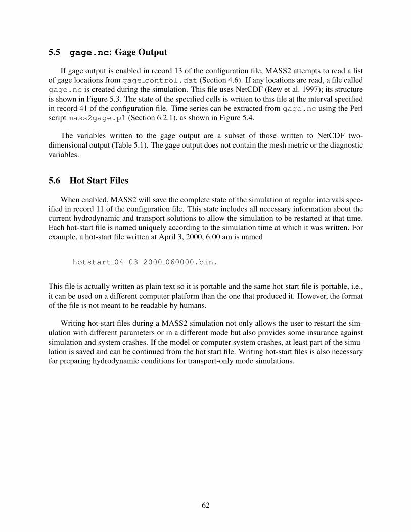
5.5 gage.nc: Gage Output
If gage output is enabled in record 13 of the configuration file, MASS2 attempts to read a list
of gage locations from gage control.dat (Section 4.6). If any locations are read, a file called
gage.nc is created during the simulation. This file uses NetCDF (Rew et al. 1997); its structure
is shown in Figure 5.3. The state of the specified cells is written to this file at the interval specified
in record 41 of the configuration file. Time series can be extracted from gage.nc using the Perl
script mass2gage.pl (Section 6.2.1), as shown in Figure 5.4.
The variables written to the gage output are a subset of those written to NetCDF two-
dimensional output (Table 5.1). The gage output does not contain the mesh metric or the diagnostic
variables.
5.6 Hot Start Files
When enabled, MASS2 will save the complete state of the simulation at regular intervals spec-
ified in record 11 of the configuration file. This state includes all necessary information about the
current hydrodynamic and transport solutions to allow the simulation to be restarted at that time.
Each hot-start file is named uniquely according to the simulation time at which it was written. For
example, a hot-start file written at April 3, 2000, 6:00 am is named
hotstart 04-03-2000 060000.bin.
This file is actually written as plain text so it is portable and the same hot-start file is portable, i.e.,
it can be used on a different computer platform than the one that produced it. However, the format
of the file is not meant to be readable by humans.
Writing hot-start files during a MASS2 simulation not only allows the user to restart the sim-
ulation with different parameters or in a different mode but also provides some insurance against
simulation and system crashes. If the model or computer system crashes, at least part of the simu-
lation is saved and can be continued from the hot start file. Writing hot-start files is also necessary
for preparing hydrodynamic conditions for transport-only mode simulations.
62

netcdf gage {
dimensions:
gage = 3 ;
time = UNLIMITED ; // (61 currently)
5 tslen = 20 ;
idlen = 40 ;
variables:
int block(gage) ;
int eta(gage) ;
10 int xi(gage) ;
char gage_name(gage, idlen) ;
double time(time) ;
time:Units = "days since 1900-01-01 00:00:00" ;
float elapsed(time) ;
15 elapsed:Units = "hours" ;
elapsed:Description = "Elapsed Simulation Time" ;
char timestamp(time, tslen) ;
float wsel(time, gage) ;
wsel:Units = "feet" ;
20 wsel:Description = "Water Surface Elevation" ;
wsel:units = "feet" ;
wsel:long_name = "Water Surface Elevation" ;
wsel:_FillValue = 9.96921e+36f ;
float depth(time, gage) ;
25 depth:Units = "feet" ;
depth:Description = "Depth" ;
depth:units = "feet" ;
depth:long_name = "Depth" ;
depth:_FillValue = 9.96921e+36f ;
30 float vmag(time, gage) ;
vmag:Units = "feet/second" ;
vmag:Description = "Velocity Magnitude" ;
vmag:units = "feet/second" ;
vmag:long_name = "Velocity Magnitude" ;
35 vmag:_FillValue = 9.96921e+36f ;
float uvel(time, gage) ;
uvel:Units = "feet/second" ;
uvel:Description = "Longitudinal Velocity" ;
uvel:units = "feet/second" ;
40 uvel:long_name = "Longitudinal Velocity" ;
uvel:_FillValue = 9.96921e+36f ;
float vvel(time, gage) ;
vvel:Units = "feet/second" ;
vvel:Description = "Lateral Velocity" ;
45 vvel:units = "feet/second" ;
vvel:long_name = "Lateral Velocity" ;
vvel:_FillValue = 9.96921e+36f ;
float isdry(time, gage) ;
isdry:Units = "none" ;
50 isdry:Description = "Dry Cell Flag" ;
isdry:units = "none" ;
isdry:long_name = "Dry Cell Flag" ;
isdry:_FillValue = 9.96921e+36f ;
}
Figure 5.3. Structure of an example NetCDF gage output file, gage.nc. This listing was pro-
duced with the NetCDF utility ncdump.
63

> perl mass2gage.pl -l gage.nc
MASS2 Gage Output File:
"gage.nc"
1 time slices:
starting: 03-19-1999 12:00:00
ending: 03-19-1999 12:00:00
Available Gage Locations
-----------------------------------------------------
Gage Name Block Eta Xi
-----------------------------------------------------
1 T54LBC piezometer 1 167 83
2 T61IRC piezometer 2 63 27
3 T64RBC piezometer 4 117 9
4 T81RBC piezometer 12 38 47
5 T90RBC piezometer 13 228 51
6 T94RBC piezometer 13 451 15
7 T101LBC piezometer 14 24 63
8 downstream extent 16 155 40
9 ERC 100-D 1 22 7
10 ERC 100-H 4 115 9
11 ERC 100-F 10 116 9
12 ERC 100-D Alternate 1 22 10
13 trouble spot 11 4 16
14 trouble spot upstream 11 3 16
15 trouble spot downstream 11 5 16
16 trouble spot west 11 4 15
17 trouble spot east 11 4 17
-----------------------------------------------------
Available Time-Dependant Variables:
8 wsel Water Surface Elevation, feet
9 depth Depth, feet
10 vmag Velocity Magnitude, feet/second
11 uvel Longitudinal Velocity, feet/second
12 vvel Lateral Velocity, feet/second
13 isdry Dry Cell Flag, none
> perl mass2gage.pl -v depth -g 8 gage.nc
03-19-1999 12:00:00 8.369
03-19-1999 13:00:00 9.9153
03-19-1999 14:00:00 9.8377
03-19-1999 15:00:00 9.7396
03-19-1999 16:00:00 9.6508
03-19-1999 17:00:00 9.562
03-19-1999 18:00:00 9.4928
Figure 5.4. Example of using the mass2gage.pl script to extract time series data from
gage.nc output. The first use of the script (in bold) produces a listing of the gage
locations and the available variables. The second use obtains the flow depth time series
for gage 8.
64

6.0 Utility Reference
Several utility programs have been developed to aid in the application of MASS2. This chapter
briefly documents the utilities that are used most often.
6.1 cartgrid Utility
The cartgrid utility is a stand-alone Fortran 90 program for generating Cartesian compu-
tational meshes for use with MASS2. The program is interactive (Figure 6.1), prompting the user
for the information needed to construct a rectangular mesh:
• longitudinal (upstream/downstream) cell spacing
• lateral (left/right bank) cell spacing
• number of longitudinal cell vertices (downstream nodes)
• number of lateral cell vertices (cross stream bank nodes)
• coordinates of the block origin (x, y)
• upstream to downstream bottom slope
• downstream bottom elevation.
Given the above information, cartgrid produces a computational mesh file named grid.out
that can be used with MASS2. The mesh describes a bed uniformly sloping from upstream to
downstream.
6.2 Perl scripts
Two utility programs have been developed to post-process MASS2 output. These programs
were written in an interpreted language called Perl.(a) The Perl interpreter is freely available and
comes with most Linux distributions. Windows distributions are also available, but the MASS2
scripts documented in this section have not been tested on Windows.
Descriptions of the programs are given below. To use them, a Perl interpreter must be available.
The utilities require Perl version 5.6 or later along with Perl Data Language (PDL) module (version
2.2 or later) and the PDL::NetCDF module (version 0.86).
(a) See http://www.perl.org.
65

> cartgrid
This program create rectangular grids.
No checks are made on data input so think before you type!
Input longitudinal spacing (delta x) desired
0.0455
Input lateral spacing (delta y) desired
0.0455
Input number of downstream nodes desired
161
Input number of cross stream nodes desired
41
Input downstream starting x coordinate
-1.820
Input starting y coordinate
0
Enter name of bottom elevation file (RETURN for none)
<enter>
Input slope
0
Input downstream bottom elevation
0
Thanks! Output file is grid.out
>
Figure 6.1. Sample cartgrid session. This session was used to produce the mesh in validation
test presented in Section 4.1.9 of the Theory Manual. The mesh was produced in
metric units first than converted to English.
Documentation for some utility scripts follows. The documentation was generated using the
Perl utility pod2latex. The documentation shown below can be seen by running perldoc on
the script file. See the Perl documentation for more information.
66

6.2.1 mass2gage.pl
Extract data from a MASS2 gage output file (NetCDF format).
SYNOPSIS
perl mass2gage.pl -l file
perl mass2gage.pl -v var -g gage [-C|-M] [-1] [-D] -X n] [-o output] file
DESCRIPTION
This script is used to extract data for one variable and gage from a MASS2 gage output file. It
is primarily intended to be used to check a simulation while in progress.
OPTIONS
-l
List the gages and time-dependant variables in file and exit.
-v var
(required) Extract the var time-dependant variable from file; var may be either an integer or
a variable name (as long as the name does not start with a number), either of which can be
obtained using -l.
-g gage
Extract data from the gage location; gage may be either an integer or a gage location name
(as long as the name does not start with a number), either of which can be obtained using -l.
-C
Output a cumulative frequency distribution; normally, a time series is output, this option will
cause the data from the specified gage to be sorted and assigned an exceedance probability.
-D
If the file contains the variable isdry, extract records for var only when isdry is zero;
applies only to the extraction of a time series; a CFD extraction will still contain all values.
-o output
Send extracted data to output (does not work with -l).
-1
Add a line at the top of the output (line 1) containing some information about the extracted
data.
67

-M
Format as a MASS1/MASS2 boundary condition file (implies -1).
-X n
Skip the first n time records in the gage file, to avoid a warm up period, for example.
EXAMPLES
This is the output from a listing (-l) of a particular gage.nc file:
> \textbf{perl mass2gage.pl -l gage.nc }
MASS2 Gage Output File:
"gage.nc"
1 time slices:
starting: 03-19-1999 12:00:00
ending: 03-19-1999 12:00:00
Available Gage Locations
-----------------------------------------------------
Gage Name Block Eta Xi
-----------------------------------------------------
1 T54LBC piezometer 1 167 83
2 T61IRC piezometer 2 63 27
3 T64RBC piezometer 4 117 9
4 T81RBC piezometer 12 38 47
5 T90RBC piezometer 13 228 51
6 T94RBC piezometer 13 451 15
7 T101LBC piezometer 14 24 63
8 downstream extent 16 155 40
9 ERC 100-D 1 22 7
10 ERC 100-H 4 115 9
11 ERC 100-F 10 116 9
12 ERC 100-D Alternate 1 22 10
13 trouble spot 11 4 16
14 trouble spot upstream 11 3 16
15 trouble spot downstream 11 5 16
16 trouble spot west 11 4 15
17 trouble spot east 11 4 17
-----------------------------------------------------
Available Time-Dependent Variables:
8 wsel Water Surface Elevation, feet
9 depth Depth, feet
68

10 vmag Velocity Magnitude, feet/second
11 uvel Longitudinal Velocity, feet/second
12 vvel Lateral Velocity, feet/second
13 isdry Dry Cell Flag, none
Depth data is extracted from the same file:
03-19-1999 12:00:00 8.369
03-19-1999 13:00:00 9.9153
03-19-1999 14:00:00 9.8377
03-19-1999 15:00:00 9.7396
03-19-1999 16:00:00 9.6508
03-19-1999 17:00:00 9.562
03-19-1999 18:00:00 9.4928
69

6.2.2 mass2slice.pl
Extract profile and cross section data from MASS2 plot output files.
SYNOPSIS
perl mass2slice.pl [-d] [-a] [-i|-j] [-t indices|-l] [-o output] file variable block index [block
index ...]
perl mass2slice.pl -p [-t indices|-l] [-o output] file variable block i j
DESCRIPTION
mass2slice.pl is used to extract slices of data from the NetCDF format MASS2 plot output file.
Slices can be made either longitudinally (-i) or laterally (-j) across multiple blocks. By default, all
times are output separated by a blank line (useful for plotting in gnuplot).
OPTIONS
-a
Average the variable across the profile or cross section to produce one value.
-d
Place the date/time in the first two columns of the output.
-D
For -i and -j slices, do not output any points where the cell is dry. This option is ignored if
there is no wet/drying information in file.
-i
Extract a profile. Distance is computed from upstream to downstream. The index is the
lateral index.
-j
Extract a cross section. Distance is computed from the right to left bank (looking down-
stream). The index is the longitudinal index.
-p
Output a timeseries at a single point rather than a slice. If this option is used, both the i and
j indices of the point (cell actually) are expected to be on the command line.
-t index
Select a specific time, specified by index, to extract. By default all times are extracted, and
their time stamp is placed in the output.
70

-l
Extract only the last time in the plot output file. The -t is ignored if this option is specified.
-o output
Send data to output instead of standard output.
EXAMPLES
This script is typically used to provide data for profile plotting. The following gnuplot script
will plot a water surface elevation profile from a three block domain:
plot ’<perl mass2slice.pl -t 1 -i plot.nc wsel 1 5 2 10 3 5’ \
using 3:4 with l 1, \
’<perl mass2slice.pl -l -i plot.nc wsel 1 5 2 10 3 5’ \
using 3:4 with l 3, \
’<perl mass2slice.pl -i plot.nc zbot 1 5 2 10 3 5’ \
using 3:4 with l 7
Block 2 is either aligned differently or of a different resolution. The resulting plot will show
three curves: the initial conditions (-t 1, wsel), the final conditions (-l, wsel), and the
bottom elevation (zbot).
SEE ALSO
gnuplot(1)
71


7.0 References
CGNS Project Group. 2003. CFD General Notation System, Overview and Entry-Level Docu-
ment. Version 2.0.7, Available URL: http://www.grc.nasa.gov/WWW/cgns/overview/index.html.
Kincaid CT, RW Bryce, PW Eslinger, CAB J. M. Becker, AL Bunn, CR Cole, EJ Freeman,
GR Guensch, DG Horton, GV Last, TB Miley, WA Perkins, WE Nichols, M Oostrom, MC Rich-
mond, DL Strenge, and PD Thorne. 2001. “Development of a Site-Wide System Assessment
Capability.” Presented at the Waste Management 2001 Symposium, February 25 - March 1,
2001, sponsored by the University of Arizona, Tuscon, Arizona.
McMichael GA, WA Perkins, CJ McMurray, YJ Chien, CL Rakowski, A Coleman, MC Rich-
mond, J Vucelick, EV Arntzen, RP Mueller, CA Duberstein, and J Lukas. 2003. Subyearling
Chinook Salmon Stranding in the Hanford Reach of the Columbia River. PNWD-3308, Battelle-
Pacific Northwest Division, P.O. Box 999, Richland, Washington 99352. Prepared for Grant
County Public Utility District No. 2.
Patankar S. 1980. Numerical Heat Transfer and Fluid Flow. Hemisphere, New York, New York.
Perkins W, M Richmond, and G McMichael. 2004. “Two-Dimensional Modeling of Time-
Varying Hydrodynamics and Juvenile Chinook Salmon Habitat in the Hanford Reach of the
Columbia River.” In Proceedings of the World Water and Environmental Resources Congress.
ASCE. Presented at conference held June 27-July 1 in Salt Lake City.
Perkins WA and MC Richmond. 2004. MASS2, Modular Aquatic Simulation System in Two
Dimensions, Theory and Numerical Methods. PNNL-14820-1, Pacific Northwest National Lab-
oratory, Richland, Washington 99352.
Rew R, G Davis, S Emmerson, and H Davies. 1997. NetCDF Users Guide for FORTRAN,
An Access Interface for Self-Describing, Portable Data. University Center for Atmospheric
Research, Unidata Program Center, P.O. Box 3000, Boulder, Colorado 80307. Available
URL: http://www.unidata.ucar.edu/packages/netcdf/fguide.pdf.
Richmond M, W Perkins, and Y Chien. 2000. Numerical Model Analysis of System-wide Dis-
solved Gas Abatement Alternatives. PNWD-3245, Battelle Pacific Northwest Division, P.O. Box
999, Richland, Washington, 99352. Prepared for the U.S. Army Corps of Engineers, Walla Walla
District under Contract DACW68-96-D-0002.
Richmond M, W Perkins, and T Scheibe. 1999. Two-Dimensional Hydrodynamic, Water Quality,
and Fish Exposure Modeling of the Columbia and Snake Rivers. Part 1: Summary and Model
Formulation. Final Report, Battelle Pacific Northwest Division, P. O. Box 999, Richland, Wash-
ington, 99352. Prepared for the U.S. Army Corps of Engineers, Walla Walla District under
Contract DACW68-96-D-0002.
Rumsey CL, DMA Poirier, RH Bush, and CE Towne. 2002. CFD General Notation
System, A User’s Guide To CGNS. CGNS Project Group. Version 1.1.4, Available
URL: http://www.grc.nasa.gov/WWW/cgns/user/index.html.
73

Spasojevic M and F Holly, Jr. 1990. “2-D Bed Evolution in Natural Watercourses New Simulation
Approach.” Journal of Waterway, Port, Coastal, and Ocean Engineering 116(4):425–443.
Steinbrenner J, N Wyman, and J Chawner. 2000a. “Development and Implementation of Grid-
gen’s Hyperbolic PDE and Extrusion Methods.” presented at the AIAA 38th Aerospace Sciences
Meeting, 10-13 Jan 2000, Reno, NV. AIAA paper no. 2000-0679.
Steinbrenner J, N Wyman, and J Chawner. 2000b. “Fast Surface Meshing on Imperfect CAD
Models.” In Proceedings of the 9th International Meshing Roundtable, 02-05 October 2000, New
Orleans, SANDIA Report SAND2000-2207, pp. 33–41.
Zender C. 2004. NCO User’s Guide. Department of Earth System Science, University of Cali-
fornia, Irvine, California. Available URL: http://nco.sourceforge.net/\#RTFM.
Zhou JG. 1995. “Velocity-Depth Coupling in Shallow-Water Flows.” Journal of Hydraulic En-
gineering 121(10):717–724.
74

Appendix A
Input Files from Validation Applications


Appendix A – Input Files from Validation Applications
In this appendix, input files for the Modular Aquatic Simulation System in Two Dimensions
(MASS2) are presented from some of the validation applications discussed in Chapter 4 of the
Theory Manual. These are presented so the that the reader may have some example input files to
use as a guide. Because of their length, computational mesh files have been omitted, but in the
applications presented, the computational mesh files were generated with the cartgrid utility
(Section 6.1) using the dimensions presented in the Theory Manual.
A.1 Subcritical, Uniform Flow in a Rectangular Channel
Section 4.1.1 of the Theory Manual presents a validation application for subcritical, uniform
flow in a rectangular channel. This problem was solved using three computational mesh blocks.
The upstream and downstream blocks were separated by a block with twice the resolution. This
application demonstrates a relatively simple application that uses one-to-many cell block connec-
tions.
mass2.cfg
1 $Id: mass2_v027.cfg,v 1.2.2.1 2004/07/22 19:53:45 perk Exp $
MASS2 Test Case: Normal Flow with grid nesting
3 ! max number of blocks
2 ! max number of species
5 "grid1.dat"
"grid2.dat"
"grid3.dat"
T ! on/off switch for hydrodynamics
F ! on/off switch for transport calculations
10 F F "weather.dat"
F ! extra debug printing
T ! manning bottom friction equation
F 1728 ! write out restart files
F ! read hotstart file
15 T ! gage output
T F ! initial: w.s. elev or depth, profile
04-01-1996 00:00:00 ! start date & time
04-01-1996 05:59:59 ! end date & time
60.0 ! time step (seconds)
20 12 10.0 ! hydro iterations, mass source error
2 ! scalar iterations
2 ! inner iterations for scalars
30 ! inner iterations for depth correction
0.20001 F ! eddy viscosity
25 0.20001 F ! diffusion coeff in xsi (ftˆ2/sec)
0.50001 F ! diffusion coeff in eta (ftˆ2/sec)
A.1

0.02600 F ! manning n value if manning=TRUE
1.49 ! constant in the bed shear stress
0.40 ! relaxation factor for depth corrections
30 0.0 ! not used
4.0 ! not used
0.2 ! initial uniform value of u velocity
0.0 ! initial uniform value of v velocity
25.0 ! initial uniform value of concentration
35 4.0 ! initial uniform value of depth OR w. s elev.
0.0 ! uniform value of u wind velocity
0.0 ! uniform value of v wind velocity
F 0.0 0.0 0.0 ! do wet/dry, dry depth, rewet depth, zero depth
0.4 0.0 F 1 ! bed: porosity, initial depth, read initial, iterations
40 1 F ! 2D output frequency, averaging
T T F ! 2D enable netcdf, diag, flow
F F T 999999 ! cgns: enable, cell centered, field desc, times/file
1 ! gage output frequency
bcspecs.dat
1 1 US TABLE FLUX ALL "flow.dat" /
1 DS BLOCK ELEV ALL 2 /
2 US BLOCK VELO ALL 1 /
2 DS BLOCK ELEV ALL 3 /
5 3 US BLOCK VELO ALL 2
3 DS TABLE ELEV ALL "stage.dat" /
flow.dat
1 # $Id: flow.dat,v 1.2 2003/05/16 22:43:32 perk Exp $
01-01-1900 00:00:00 5000.0 /
01-01-2000 00:00:00 5000.0 /
stage.dat
1 # $Id: stage.dat,v 1.2 2003/05/16 22:43:34 perk Exp $
01-01-1900 00:00:00 5.0 /
01-01-2000 00:00:00 5.0 /
A.2

A.2 Two-Dimensional Flow Around a Spur Dike
Section 4.1.8 of the Theory Manual presents a validation test from the literature for two-
dimensional flow around a spur dike. The shell script mkgrid.sh shown on page A.3 used
the cartgrid to generate the single computational mesh block used in this application. The
mkgrid.sh script generated the grid with metric dimensions, then converted to English. The
spur dike was represented using a wall boundary condition (Section 4.3.3), as shown in the
bcspecs.dat file on page A.4.
mkgrid.sh
1 #! /bin/sh
# -------------------------------------------------------------
# file: mkgrid.sh
# -------------------------------------------------------------
5 # -------------------------------------------------------------
# Battelle Memorial Institute
# Pacific Northwest Laboratory
# -------------------------------------------------------------
# -------------------------------------------------------------
10 # Created October 8, 2003 by William A. Perkins
# -------------------------------------------------------------
# dimensions in meters
15 L=5.4
W=0.9
nx=217
ny=37
dx=‘echo scale=6\;$L/\($nx - 1\) | bc‘
20 dy=‘echo scale=6\;$W/\($ny - 1\) | bc‘
../../../util/cart_grid/cartgrid <<EOF
$dx ! longitudinal spacing
$dy ! lateral spacing
25 $nx ! downstream nodes
$ny ! cross stream nodes
0.0 ! starting x coordinate
0.0 ! starting y coordinate
30 5.9014e-05 ! slope
0.0 ! downstream elevation
EOF
awk -f - grid.out > grid.dat <<EOF
35 NF == 5 {
x = \$3/0.3048;
y = \$4/0.3048;
z = \$5/0.3048;
printf("%5d %5d %12.6g %12.6g %12.6g\n", \$1, \$2, x, y, z);
40 next;
}
A.3

{ print; }
EOF
mass2.cfg
1 $Id: mass2_v027.cfg,v 1.3.2.1 2004/07/22 19:53:44 perk Exp $
MASS2 Test Case: Two dimensional flow around a spur dike.
1 ! max number of blocks
1 ! max number of species
5 "grid.dat"
T ! on/off switch for hydrodynamics
F ! on/off switch for transport calculations
F F "weather.dat"
F ! extra debug printing
10 T ! manning bottom friction equation
T 100000 ! write out restart files
F ! read hotstart file
T ! gage output
T F ! initial: w.s. elev or depth, profile
15 04-01-1996 00:00:00 ! start date & time
04-01-1996 00:05:00 ! end date & time
0.25 ! time step (seconds)
5 0.001 ! hydro iterations, mass source error
2 ! scalar iterations
20 2 ! inner iterations for scalars
25 ! inner iterations for depth correction
1.61e-02 F ! eddy viscosity
0.20001 F ! diffusion coeff in xsi (ftˆ2/sec)
0.50001 F ! diffusion coeff in eta (ftˆ2/sec)
25 0.0100 F ! manning n value if manning=TRUE
1.49 ! constant in the bed shear stress
0.20 ! relaxation factor for depth corrections
0.0 ! not used
0.62 ! not used
30 0.0 ! initial uniform value of u velocity
0.0 ! initial uniform value of v velocity
25.0 ! initial uniform value of concentration
0.62 ! initial uniform value of depth OR w. s elev.
0.0 ! uniform value of u wind velocity
35 0.0 ! uniform value of v wind velocity
T 0.01 0.015 0.005 ! do wet/dry, dry depth, rewet depth, zero depth
0.4 0.0 F 1 ! bed: porosity, initial depth, read initial, iterations
999999 F ! 2D output frequency, averaging
T T F ! 2D enable netcdf, diag, flow
40 F F T 999999! cgns: enable, cell centered, field desc, times/file
4 ! gage output frequency
bcspecs.dat
1 1 US TABLE FLUX ALL "flow.dat" /
1 IN WALL UVEL 73 1 6 /
1 DS TABLE ELEV ALL "stage.dat" /
A.4

flow.dat
1 # Constant flow
01-01-1900 00:00:00 1.5198 /
01-01-3000 00:00:00 1.5198 /
stage.dat
1 # $Id: stage.dat,v 1.1 2003/10/24 20:00:35 perk Exp $
01-01-1900 00:00:00 0.620 /
01-01-3000 00:00:00 0.620 /
A.5

A.3 Lateral Mixing
This scalar transport application was presented in Section 4.2.3 of the Theory Manual. In
this single block application, the hydrodynamic conditions were subcritical and uniform. The
configuration file and hydrodynamics files are shown below. The transport of a single scalar was
simulated; see the scalar source.dat file on page A.7. Two concentrations were applied at
the upstream boundary, as shown in the scalar bcspecs.dat file on pageA.7.
A.3.1 Hydrodynamics Input Files
mass2.cfg
1 $Id: mass2_v027.base,v 1.4.2.1 2004/07/22 19:53:44 perk Exp $
MASS2 Test Case: Mixing of two streams
1 ! max number of blocks
1 ! max number of species
5 "grid.dat"
T ! on/off switch for hydrodynamics
T ! on/off switch for transport calculations
F F "weather.dat"
F ! extra debug printing
10 T ! manning bottom friction equation
F 1728 ! write out restart files
F ! read hotstart file
T ! gage output
T F ! initial: w.s. elev or depth, profile
15 04-01-1996 00:00:00 ! start date & time
04-01-1996 05:59:59 ! end date & time
60.0 ! time step (seconds)
10 10.0 ! hydro iterations, mass source error
2 ! scalar iterations
20 2 ! inner iterations for scalars
50 ! inner iterations for depth correction
0.20001 F ! eddy viscosity
0.20001 F ! diffusion coeff in xsi (ftˆ2/sec)
3.00000 F ! diffusion coeff in eta (ftˆ2/sec)
25 0.026 F ! manning n value if manning=TRUE
1.49 ! constant in the bed shear stress
0.40 ! relaxation factor for depth corrections
0.0 ! not used
6.0 ! not used
30 0.2 ! initial uniform value of u velocity
0.0 ! initial uniform value of v velocity
0.0 ! initial uniform value of concentration
6.0 ! initial uniform value of depth OR w. s elev.
0.0 ! uniform value of u wind velocity
35 0.0 ! uniform value of v wind velocity
F 0.0 0.0 0.0 ! do wet/dry, dry depth, rewet depth, zero depth
0.4 0.0 F 1 ! bed: porosity, initial depth, read initial, iterations
360 F ! 2D output frequency, averaging
T T F ! 2D enable netcdf, diag, flow
40 F F T 999999 ! cgns: enable, cell centered, field desc, times/file
A.6

10 ! gage output frequency
bcspecs.dat
1 1 US TABLE FLUX ALL "flow.dat" /
1 DS TABLE ELEV ALL "stage.dat" /
flow.dat
1 # $Id: flow.dat,v 1.2 2001/11/29 18:16:00 perk Exp $
01-01-1900 00:00:00 1000.0 /
01-01-2000 00:00:00 1000.0 /
stage.dat
1 # $Id: stage.dat,v 1.2 2001/11/29 18:16:15 perk Exp $
01-01-1900 00:00:00 6.0 /
01-01-2000 00:00:00 6.0 /
A.3.2 Transport Input Files
scalar source.dat
1 1 GEN stuff "Conservative transportable stuff" "bulldogs/liter" /
scalar bcspecs.dat
1 1 US TABLE 1 CONC PART "conc.dat" 1 1 10 /
1 US TABLE 1 CONC PART "bkgnd.dat" 1 11 20 /
1 DS ZEROG 1 CONC ALL /
bkgnd.dat
1 # $Id: bkgnd.dat,v 1.2 2001/11/29 18:15:59 perk Exp $
01-01-1900 00:00:00 100.0 /
01-01-2000 00:00:00 100.0 /
conc.dat
1 # $Id: conc.dat,v 1.2 2001/11/29 18:15:59 perk Exp $
01-01-1900 00:00:00 200.0 /
01-01-2000 00:00:00 200.0 /
A.7


Appendix B
Example Applications


Appendix B – Example Applications
In this appendix, several “real-world” applications of the Modular Aquatic Simulation System
in Two Dimensions (MASS2) are described. This appendix is included to showcase some interest-
ing MASS2 applications, provide examples of input files when interesting MASS2 features were
used.
B.1 McNary Pool Dissolved Gas
As part of the U. S. Army Corps of Engineers’ (USACE) Dissolved Gas Abatement (DGAS)
Program, MASS2 was applied to the parts of the Columbia and Snake rivers impounded by
McNary Dam, located on the Columbia River near Umatilla, Oregon. The application extended
from Clover Island to McNary Dam on the Columbia River and from Ice Harbor Dam on the Snake
River to its confluence with the Columbia River. Additional information on this application can be
found in Richmond et al. (1999). The computational grid consisted of 13 blocks (Figure B.1) and
covered over 78,000 acres, with an average resolution of 147 ft laterally and 330 ft longitudinally
(Table B.1).
This application was developed to simulate the fate of total dissolved gas (TDG) generated
at Ice Harbor Dam. It used the temperature and TDG simulation capabilities of MASS2. In the
hydrodynamics, Ice Harbor Dam discharge was divided between spillway and power house, as
shown in lines 1-2 of the bcspecs.dat file (page B.5). Several small spoil islands that were not
resolved in the computational mesh were represented by an area with higher roughness, as shown
in the roughness coeff.dat file on page B.5.
Water that spills through the Ice Harbor Dam spillway entrains gas. The amount of entrainment
was estimated. In scalar bcspecs.dat (shown on page B.6), the boundary at the dam was
split into two parts so different gas concentrations could be applied at the spillway and power house
(lines 1 and 2). The same water temperature was applied over the entire dam boundary (line 10).
Gas exchange coefficients (page B.6) were adjusted during calibration.
B.1

13
12
10
11
9
12
3
4
6
5
7
8
McNary Dam
Ice Harbor Dam
Columbia River
Snake River
Figure B.1. Computational mesh block arrangement for the McNary Pool dissolved gas applica-
tion.
B.2

Table B.1. Size and resolution statistics for the MASS2 computational grid
for the McNary Pool dissolved gas application.
Cell Size, feet Block
Lateral Longitudinal Area
Block Cells Min Avg Max Min Avg Max (acre)
1 1449 37 68 182 46 96 182 323
2 352 63 81 104 97 123 172 123
3 154 39 71 182 73 138 224 68
4 1701 61 88 210 76 221 375 1975
5 288 75 118 193 95 225 315 348
6 540 36 98 189 97 218 366 625
7 945 45 108 320 26 263 493 1662
8 1281 88 159 268 52 315 513 3041
9 1000 53 116 320 32 346 517 3285
10 2480 54 186 382 99 399 750 9973
11 1071 111 236 563 105 246 630 1615
12 4189 94 200 657 58 374 662 14418
13 12360 79 140 400 92 372 601 40569
all 27810 36 147 657 26 330 750 78024
B.3

mass2.cfg
1 mass2 version 0.27 configuration base file
FINS McNary Pool Simulation - Benchmark Simulation
13 max number of blocks
2 max number of species
5 "grid-3/grid-pt.013-1.dat"
"grid-3/grid-pt.000.dat"
"grid-3/grid-pt.001.dat"
"grid-3/grid-pt.002.dat"
"grid-3/grid-pt.003.dat"
10 "grid-3/grid-pt.004.dat"
"grid-3/grid-pt.005.dat"
"grid-3/grid-pt.006.dat"
"grid-3/grid-pt.007a.dat"
"grid-3/grid-pt.007b.dat"
15 "grid-3/grid-pt.009.dat"
"grid-3/grid-pt.008.dat"
"grid-3/grid-pt.010-all.dat"
T ! on/off switch for hydrodynamics
T ! on/off switch for transport calculations
20 T T "BCFiles/MCN_Weather.prn"
F ! extra debug printing
T ! manning bottom friction equation
F 18 ! write out restart files
T ! read hotstart file
25 T ! no gage output
T F ! initial: w.s. elev or depth, profile
05-20-1997 12:00:00 ! start date & time
05-20-1997 16:00:00 ! end date & time
50.0 ! time step (seconds)
30 6 3000.0 ! hydro iterations, mass source error
2 ! scalar iterations
2 ! inner iterations for scalars
15 ! inner iterations for depth correction
0.20001 F ! eddy viscosity
35 0.20001 F ! diffusion coeff in xsi (ftˆ2/sec)
0.50001 F ! diffusion coeff in eta (ftˆ2/sec)
0.027 T ! manning n value if manning=TRUE
1.49 ! constant in the bed shear stress
0.40 ! relaxation factor for depth corrections
40 0.0 ! not used
338.3 ! not used
0.2 ! initial uniform value of u velocity
0.0 ! initial uniform value of v velocity
25.0 ! initial uniform value of concentration
45 338.3 ! initial uniform value of depth OR w. s elev.
0.0 ! uniform value of u wind velocity
0.0 ! uniform value of v wind velocity
F 0.0 0.0 0.0 ! do wet/dry, dry depth, rewet depth, zero depth
0.4 0.0 F 1 ! bed: porosity, initial depth, read initial, iterations
50 72 F ! 2D output frequency, averaging
T T F ! 2D enable netcdf, diag, flow
T F T 999999! cgns: enable, cell centered, field desc, times/file
B.4

1 ! gage output frequency
bcspecs.dat
1 1 US TABLE FLUX PART "BCFiles/IHR_QS.prn" 1 10 /
1 US TABLE FLUX PART "BCFiles/IHR_QP.prn" 11 19 /
1 DS BLOCK ELEV PART 2 1 14 /
1 DS BLOCK ELEV PART 3 15 19 /
5 2 US BLOCK VELO ALL 1 /
2 DS BLOCK ELEV ALL 4 /
3 US BLOCK VELO ALL 1 /
3 DS BLOCK ELEV ALL 4 /
4 US BLOCK VELO PART 2 1 14 /
10 4 US BLOCK VELO PART 3 15 19 /
4 DS BLOCK ELEV PART 5 1 6 /
4 DS BLOCK ELEV PART 6 7 19 /
5 US BLOCK VELO ALL 4 /
5 DS BLOCK ELEV ALL 7 /
15 6 US BLOCK VELO ALL 4 /
6 DS BLOCK ELEV ALL 7 /
7 US BLOCK VELO PART 5 1 6 /
7 US BLOCK VELO PART 6 7 19 /
7 DS BLOCK ELEV ALL 9 /
20 8 US TABLE FLUX PART "BCFiles/zeroflow.dat" 1 9 /
8 US TABLE FLUX PART "BCFiles/Clover_Q.prn" 10 19 /
8 DS BLOCK ELEV ALL 9 /
9 US BLOCK VELO PART 8 1 19 /
9 US BLOCK VELO PART 7 20 38 /
25 9 DS TABLE VELO PART "BCFiles/zeroflow.dat" 24 38 /
9 DS BLOCK ELEV PART 10 1 23 /
10 US BLOCK VELO PART 9 1 23 /
10 US TABLE FLUX PART "BCFiles/zeroflow.dat" 24 38 /
10 DS BLOCK ELEV ALL 12 /
30 11 US TABLE FLUX ALL "BCFiles/zeroflow.dat" /
11 DS BLOCK ELEV ALL 12 /
12 US BLOCK VELO PART 10 1 38 /
12 US BLOCK VELO PART 11 39 57 /
12 DS TABLE VELO PART "BCFiles/zeroflow.dat" 39 57 /
35 12 DS BLOCK ELEV PART 13 1 38 /
13 US BLOCK VELO ALL 12 /
13 DS TABLE ELEV ALL "BCFiles/MCN_FBZ.prn" /
roughness coeff.dat
1 9 .045 14 21 24 29 /
scalar source.dat
1 1 TDG tdgconc "Total Dissolved Gas" "mg/l" AIREXCH
PARAMETERS "gas_exchange_coeff.dat" /
2 TEMP temperature "Water Temperature" Celcius AIREXCH /
B.5

scalar bcspecs.dat
1 1 US TABLE 1 CONC PART "BCFiles/IHR_CS.prn" 1 1 10 /
1 US TABLE 1 CONC PART "BCFiles/IHR_CP.prn" 1 11 19 /
8 US TABLE 1 CONC ALL "BCFiles/Clover_C.prn" 1 /
8 US ZEROG 1 CONC PART 1 9 /
5 9 DS ZEROG 1 CONC PART 24 38 /
10 US ZEROG 1 CONC PART 24 38 /
11 US ZEROG 1 CONC ALL /
12 DS ZEROG 1 CONC PART 39 57 /
13 DS ZEROG 1 CONC ALL /
10 1 US TABLE 2 CONC ALL "BCFiles/IHR_T.prn" 1 /
8 US TABLE 2 CONC ALL "BCFiles/Clover_T.prn" 1 /
8 US ZEROG 2 CONC PART 1 9 /
9 DS ZEROG 2 CONC PART 24 38 /
10 US ZEROG 2 CONC PART 24 38 /
15 11 US ZEROG 2 CONC ALL /
12 DS ZEROG 2 CONC PART 39 57 /
13 DS ZEROG 2 CONC ALL /
gas exchange coeff.dat
1 0.6885 -0.5025 0.1535 -0.0045 / a, b, c, d
B.2 Hanford Reach Hydrodynamics
In this application, MASS2 was used to simulate hydrodynamics in the Hanford Reach of
the Columbia River. The simulated hydrodynamics were used to estimate juvenile fall Chinook
habitat area and the portion of that area affected by rapid discharge fluctuations, as described by
McMichael et al. (2003) and Perkins et al. (2004). MASS2 was configured to simulate approx-
imately 23 miles of the Columbia River along the Hanford Reach from river mile (RM) 355 to
378. The computational mesh was composed of 16 blocks, as shown in Figure B.2, encompassed
approximately 7800 acres, and used more than 224,000 cells (Table B.2). The grid resolution
averaged 31 feet laterally and 49 feet longitudinally.
This MASS2 application is an example of using wetting and drying and using an initial water
surface profile for the cold start simulation. The configuration file shown (page B.10) is that used
for the initial cold start simulation. The cold start used an initial water surface profile simulated
by a previously applied one-dimensional model (Perkins et al. 2002) and supplied to MASS2 in
the initial specs.dat file (page B.12). Hydrodynamic solution and wetting and drying
parameters were varied as shown in Table B.3.
The boundary conditions required for MASS2 were total river discharge upstream and stage
downstream. These were also supplied by the one-dimensional model which was used to simulate
the Hanford Reach for the same periods as MASS2. The discharge and stage simulated by that
model were extracted at the appropriate locations and used for MASS2 boundary conditions.
MASS2 was calibrated for the simulated region by adjusting the value of Manning’s n until
simulated stage closely matched the stage observed at three water level monitors operated by
B.6

100FArea
100DArea
100HArea
16
15
14
13
12
11
10
8
97
6
1
5
4
3
2
Figure B.2. Computational mesh blocks for simulation of Hanford Reach hydrodynamics.
the U.S. Department of Energy on the Hanford Reservation. The domain was divided into three
areas between these stage monitors in which a single value of Manning’s n was used (see the
roughness coeff.dat file on page B.13). The gage control.dat file (page B.12) was
used to specify the location of 10 stage recorder locations. One of these locations (ERC 100-D)
became dry more often than the stage recorder, so an alternative location, farther in to the river,
was also used. The gage location on line 7 was used to check that the downstream stage boundary
conditions were appropriately applied.
Computationally, this was a relatively large problem, not just in space (i.e., number of cells) but
also in time. This led to two problems while performing these multi-month simulations. The first
was long execution time. On the fastest computers available to this work (Intel Pentium IV with
clock speed greater than 2.0 gigahertz), it took about 6 to 8 hours to simulate a single day. This
meant that simulating 60 days would have taken 15 to 20 days if such a processor were available
for that length of time. The second problem was the space required to store hourly results. With
the current MASS2 output options, a five-day simulation produced a results file that was too large
for the computer system.
These problems were solved by dividing each simulation period into four-day periods. The
simulation of each four-day period was started 12 hours early, allowing the simulation to transition
B.7

Table B.2. Size and resolution statistics for the MASS2 computational grid
for the Hanford Reach hydrodynamics application.
Cell Size, feet Block
Lateral Longitudinal Area
Block Cells Min Avg Max Min Avg Max (acre)
1 24120 19 34 111 22 53 86 1597
2 4641 22 27 37 26 40 56 172
3 4715 25 48 90 22 51 86 297
4 14400 18 39 83 25 53 88 977
5 4386 32 38 68 35 51 80 268
6 12300 13 29 60 18 29 82 255
7 3542 24 39 51 30 46 58 170
8 2821 42 58 74 32 46 58 135
9 9380 24 47 94 17 41 70 395
10 25110 14 29 95 22 45 83 1251
11 2318 14 30 55 37 53 70 152
12 8103 25 48 80 22 66 97 826
13 66870 14 27 73 22 49 87 3639
14 24095 13 19 31 23 56 70 1737
15 3263 20 36 71 37 76 117 433
16 14220 18 30 62 31 45 77 667
all 224284 13 31 111 17 49 117 7978
Table B.3. Parameters used for simulation of Hanford Reach hydrodynamics.
Time Hydro. Mass Src. Eddy Under- Dry Rewet Zero
Step Iter. Error Visc. relaxation Depth Depth Depth
(s) (cfs) (ft2/s) (ft) (ft) (ft)
Cold start 1.0 3 3000.0 10.2 0.05 0.4 0.45 0.20
Warm up 15.0 15 3000.0 0.2 0.15 0.3 0.35 0.18
Simulation 16.0 12 8000.0 0.2 0.30 0.3 0.35 0.18
Simulation(a) 12.0 12 8000.0 0.2 0.30 0.3 0.35 0.18
Simulation(b) 10.0 12 8000.0 0.2 0.30 0.3 0.35 0.18
(a) Only used when simulations run with a 16.0 s time step became unstable.
(b) Only used when simulations run with a 12.0 s time step became unstable.
B.8

from starting conditions before simulation results were used. Several of these four-day periods
were run simultaneously on several computers using the same starting conditions. In this way, the
season simulation for a single scenario took about one week to complete, depending on the number
and speed of available processors.
With this approach, the in-river area was simulated consistently, because of the 12-hour warm
up. Simulated conditions within the river at the end of one four-day period matched those at the be-
ginning of the next four-day period. However, the simulated time histories of any pools entrapped
outside the river were not simulated consistently. One would expect the smaller entrapped pools
to dry up over time due to evaporation and drainage. The rate at which these pools dry would
be related to the weather, properties of their substrate material, and the distance from and height
difference with the main river channel. Data to determine these drainage rates were not available.
Given these complications, it was beyond the scope of this work to produce an accurate time his-
tory for pools outside the main river channel. Consequently, the time histories of pools outside
were ignored in the analysis of simulation results.
B.9

mass2.cfg
1 mass2 version 0.25 configuration file
Grant County Stranding - Coarse Grid Setup, complete reach
16 max number of blocks
2 max number of species
5 "../grid/hanf50c-pt.000" ! 1
"../grid/hanf50c-pt.010" ! 2
"../grid/hanf50c-pt.009" ! 3
"../grid/hanf50c-pt.011" ! 4
"../grid/hanf50c-pt.001" ! 5
10 "../grid/hanf50c-pt.002" ! 6
"../grid/hanf50c-pt.003" ! 7
"../grid/hanf50c-pt.004" ! 8
"../grid/hanf50c-pt.005" ! 9
"../grid/hanf50c-pt.006" ! 10
15 "../grid/hanf50c-pt.007" ! 11
"../grid/hanf50c-pt.008" ! 12
"../grid/hanf50c-pt.013" ! 13
"../grid/hanf50c-pt.014" ! 14
"../grid/hanf50c-pt.012" ! 15
20 "../grid/hanf50c-pt.015" ! 16
T ! on/off switch for hydrodynamics
F ! on/off switch for transport calculations
F F "./BCFiles/pasco_weather.prn"
F ! extra debug output
25 T ! manning bottom friction equation
T 3600 ! write out restart files
F ! read hotstart file
T ! no gage output
T T ! initial: w.s. elev or depth, profile
30 03-01-2002 00:00:00 ! start date & time
03-01-2002 06:00:00 ! end date & time
1.0 ! time step (seconds)
2 3000.0 ! hydro iterations, mass source error
2 ! scalar iterations
35 5 ! inner iterations for scalars
25 ! inner iterations for depth correction
10.20001 F ! eddy viscosity (ftˆ2/sec)
0.20001 F ! diffusion coeff in xsi (ftˆ2/sec)
0.50001 F ! diffusion coeff in eta (ftˆ2/sec)
40 0.025 F ! manning n value if manning=TRUE
1.49 ! constant in bed shear stress
0.05 ! relaxation factor for depth corrections
0.0 ! not used
379.35 ! not used
45 0.5 ! initial uniform value of u velocity
B.10

0.0 ! initial uniform value of v velocity
25.0 ! initial uniform value of concentration
394.5 ! initial uniform value of depth OR w. s elev.
0.0 ! uniform value of u wind velocity
50 0.0 ! uniform value of v wind velocity
T 0.40 0.45 0.20 ! do wet/dry, dry depth, rewet depth, zero depth
0.4 0.0 F 1 ! bed: porosity, initial depth, read initial, iterations
3600 F ! 2D output frequency, averaging
F T F ! 2D enable netcdf, diag, flow
55 T F T 999999 ! cgns: enable, cell centered, field desc, times/file
1 ! gage output frequency
bcspecs.dat
1 1 US TABLE FLUX ALL "./BCFiles/flow.dat" /
1 DS BLOCK ELEV PART 2 1 49 /
1 DS BLOCK ELEV PART 3 50 88 /
2 US BLOCK VELO ALL 1 /
5 2 DS BLOCK ELEV ALL 4 /
3 US BLOCK VELO ALL 1 /
3 DS BLOCK ELEV ALL 4 /
4 US BLOCK VELO PART 2 1 49 /
4 US BLOCK VELO PART 3 50 88 /
10 4 DS BLOCK ELEV PART 5 1 49 /
4 DS BLOCK ELEV PART 6 50 88 /
5 US BLOCK VELO ALL 4 /
5 DS BLOCK ELEV PART 7 1 20 /
5 DS BLOCK ELEV PART 8 21 49 /
15 6 US BLOCK VELO ALL 4 /
6 DS BLOCK ELEV ALL 9 /
7 US BLOCK VELO ALL 5 /
7 DS BLOCK ELEV ALL 10 /
8 US BLOCK VELO ALL 5 /
20 8 DS BLOCK ELEV ALL 9 /
9 US BLOCK VELO PART 8 1 29 /
9 US BLOCK VELO PART 6 30 68 /
9 DS BLOCK ELEV ALL 10 /
10 US BLOCK VELO PART 7 1 20 /
25 10 US BLOCK VELO PART 9 21 88 /
10 DS BLOCK ELEV PART 11 1 17/
10 DS BLOCK ELEV PART 12 18 88/
11 US BLOCK VELO ALL 10 /
11 DS BLOCK ELEV ALL 13 /
30 12 US BLOCK VELO ALL 10/
12 DS BLOCK ELEV ALL 13 /
13 US BLOCK VELO PART 11 1 17 /
B.11

13 US BLOCK VELO PART 12 18 88 /
13 DS BLOCK ELEV PART 14 1 77 /
35 13 DS BLOCK ELEV PART 15 78 88 /
14 US BLOCK VELO ALL 13/
14 DS BLOCK ELEV ALL 16/
15 US BLOCK VELO ALL 13 /
15 DS BLOCK ELEV ALL 16 /
40 16 US BLOCK VELO PART 14 1 77 /
16 US BLOCK VELO PART 15 78 88 /
16 DS TABLE ELEV ALL "./BCFiles/stage.dat" /
initial specs.dat
1 "Initial/p50b-pt.000" / ! 1
"Initial/p50b-pt.010" / ! 2
"Initial/p50b-pt.009" / ! 3
"Initial/p50b-pt.011" / ! 4
5 "Initial/p50b-pt.001" / ! 5
"Initial/p50b-pt.002" / ! 6
"Initial/p50b-pt.003" / ! 7
"Initial/p50b-pt.004" / ! 8
"Initial/p50b-pt.005" / ! 9
10 "Initial/p50b-pt.006" / ! 10
"Initial/p50b-pt.007" / ! 11
"Initial/p50b-pt.008" /! 12
"Initial/p50b-pt.013" /! 13
"Initial/p50b-pt.014" /! 14
15 "Initial/p50b-pt.012" /! 15
"Initial/p50b-pt.015" /! 16
gage control.dat
1 1 167 83 "T54LBC piezometer" / T54LBC piezometer
2 63 27 "T61IRC piezometer" / T61IRC piezometer
4 117 9 "T64RBC piezometer" / T64RBC piezometer
12 38 47 "T81RBC piezometer" / T81RBC piezometer
5 13 228 51 "T90RBC piezometer" / T90RBC piezometer
13 451 15 "T94RBC piezometer" / T94RBC piezometer
14 24 63 "T101LBC piezometer" / T101LBC piezometer
16 155 40 "downstream extent" / downstream extent
1 22 7 "ERC 100-D" / ERC 100-D
10 4 115 9 "ERC 100-H" / ERC 100-H
10 116 9 "ERC 100-F" / ERC 100-F
1 22 10 "ERC 100-D Alternate" /
B.12

roughness coeff.dat
1 1 0.0266 1 267 1 89
2 0.0266 1 90 1 50
3 0.0266 1 114 1 40
4 0.0266 1 125 1 89
5 4 0.0278 126 159 1 89
5 0.0278 1 85 1 50
6 0.0278 1 299 1 40
7 0.0278 1 160 1 21
8 0.0278 1 90 1 30
10 9 0.0278 1 133 1 69
10 0.0278 1 123 1 89
10 0.0259 124 278 1 89
11 0.0259 1 121 1 89
12 0.0259 1 110 1 72
15 13 0.0259 1 741 1 89
14 0.0259 1 304 1 78
15 0.0259 1 250 1 12
16 0.0259 1 157 1 89
B.3 System Assessment Capability Application
MASS2 is a component of the System Assessment Capability (SAC) (Kincaid et al. 2001).
MASS2 is used to simulate the fate of radionuclides and other contaminants that have already or
may enter the Columbia river from various sources on the U.S. Department of Energy Hanford
Reservation. Because very long periods are simulated with SAC (1000 to 10,000 years), a coarse
mesh was used. The computational mesh consisted of 57 blocks (Figure B.3) and about 4600
cells and covered about 18,000 acres (Table B.4). MASS2’s transport-only mode was utilized to
increase performance (at the expense of accuracy and completeness, perhaps).
Monthly mean discharges were used to provide the hydrodynamic conditions for transport
only mode. In advance, the monthly mean discharge was simulated as a steady-state discharge for
about 45 years of record. The hydrodynamic input files presented (Section B.3.1) are for one such
monthly mean discharge.
In the transport input files (Section B.3.2), a single sediment fraction and the ra-
dionuclide Technetium-99 in dissolved and particulate phases were simulated (see the
scalar bcspecs.dat file on page B.24). A bed source is used to represent a
source of Technetium-99 brought to the river through groundwater (lines 11 and 12 of
scalar bcspecs.dat). This was estimated with a groundwater flow and transport model.
The groundwater model produced a contaminant and water flux at a number of locations. The
same locations were used for both contaminant and water flux, which is why the same map file is
used for both the BEDSOURCE (line 11) and BEDFLOW (line 12) records.
B.13

Figure B.3. Computational mesh block layout for the System Assessment Capability application.
B.14

Table B.4. Size and resolution statistics for the MASS2 computational grid.
Cell Size, feet Block
Lateral Longitudinal Area
Block Cells Min Avg Max Min Avg Max (acre)
1 48 77 118 178 254 928 1371 1041
2 42 78 121 170 277 1035 1744 1192
3 30 116 159 210 420 708 1273 384
4 96 89 138 461 426 1017 1265 2424
5 64 129 167 469 277 644 1219 737
6 40 117 137 159 277 771 1395 634
7 40 166 209 947 362 756 2044 755
8 25 188 235 301 395 670 1395 334
9 77 99 183 286 661 1530 2056 4351
10 121 103 152 302 442 1251 1397 4519
11 35 80 136 189 637 854 1046 594
12 78 95 150 414 512 901 1409 1509
13 30 94 120 154 498 645 945 304
14 54 154 192 213 805 1163 1411 1716
15 54 103 142 501 236 723 927 689
16 42 69 129 226 147 699 941 506
17 20 87 105 116 236 552 1065 188
18 72 73 137 739 119 763 1391 1125
19 72 83 97 121 439 767 915 987
20 80 129 158 198 384 975 1228 1827
21 80 104 147 511 738 948 1542 1752
22 64 100 145 172 763 1390 1542 2920
23 80 98 139 655 604 1167 1414 2596
24 35 127 161 205 596 894 1439 727
25 55 58 140 188 831 978 1439 1230
26 91 100 135 457 644 1159 1542 2877
27 112 58 131 727 772 1012 1293 2667
28 80 82 139 214 796 946 1135 1652
29 48 158 196 216 846 967 1313 1046
30 42 66 118 165 794 1076 1313 1128
31 143 79 142 473 868 1028 1270 3478
32 144 103 156 481 876 1040 1221 3582
33 64 94 114 139 585 1104 1241 1828
34 80 120 163 227 537 1076 1165 2166
35 64 109 185 505 537 910 1217 1295
36 90 97 143 203 562 1066 1210 2434
37 72 99 153 220 580 1047 1176 1872
38 64 116 175 526 548 965 1404 1508
39 72 144 163 184 518 1225 1430 2657
40 90 121 163 220 630 1252 1444 3436
41 64 156 199 473 517 875 1444 1277
42 60 113 195 430 268 741 1036 798
43 48 154 181 204 640 910 1209 935
44 36 113 145 195 800 969 1038 780
45 24 284 304 329 245 615 1209 274
46 72 178 214 637 272 958 1188 1575
47 495 123 189 351 648 1313 1593 19746
48 64 83 138 563 254 798 1442 1177
49 80 101 176 663 687 1051 1681 2124
50 144 112 206 352 558 917 1271 2844
51 80 64 106 571 558 803 1031 1219
52 369 115 205 350 108 1200 1633 12677
53 144 174 250 356 800 1373 1555 6342
54 64 81 117 336 384 873 1618 1367
55 64 107 155 500 108 584 1214 712
56 64 158 182 375 800 1041 1483 1634
57 40 117 193 1099 265 561 1545 369
4602 58 166 1099 108 1040 2056 18391
B.15

B.3.1 Hydrodynamics Input Files
mass2.cfg
1 mass2 version 0.25 configuration file
Checking block connections for Hanford Reach
57 max number of blocks
2 max number of species
5 "../new_sac_grid/sac_n-pt.001"
"../new_sac_grid/sac_n-pt.002"
"../new_sac_grid/sac_n-pt.003"
"../new_sac_grid/sac_n-pt.004"
"../new_sac_grid/sac_n-pt.005"
10 "../new_sac_grid/sac_n-pt.006"
"../new_sac_grid/sac_n-pt.007"
"../new_sac_grid/sac_n-pt.008"
"../new_sac_grid/sac_n-pt.009"
"../new_sac_grid/sac_n-pt.010"
15 "../new_sac_grid/sac_n-pt.011"
"../new_sac_grid/sac_n-pt.012"
"../new_sac_grid/sac_n-pt.013"
"../new_sac_grid/sac_n-pt.014"
"../new_sac_grid/sac_n-pt.015"
20 "../new_sac_grid/sac_n-pt.016"
"../new_sac_grid/sac_n-pt.017"
"../new_sac_grid/sac_n-pt.018"
"../new_sac_grid/sac_n-pt.019"
"../new_sac_grid/sac_n-pt.020"
25 "../new_sac_grid/sac_n-pt.021"
"../new_sac_grid/sac_n-pt.022"
"../new_sac_grid/sac_n-pt.023"
"../new_sac_grid/sac_n-pt.024"
"../new_sac_grid/sac_n-pt.025"
30 "../new_sac_grid/sac_n-pt.026"
"../new_sac_grid/sac_n-pt.027"
"../new_sac_grid/sac_n-pt.028"
"../new_sac_grid/sac_n-pt.029"
"../new_sac_grid/sac_n-pt.030"
35 "../new_sac_grid/sac_n-pt.031"
"../new_sac_grid/sac_n-pt.032"
"../new_sac_grid/sac_n-pt.033"
"../new_sac_grid/sac_n-pt.034"
"../new_sac_grid/sac_n-pt.035"
40 "../new_sac_grid/sac_n-pt.036"
"../new_sac_grid/sac_n-pt.037"
"../new_sac_grid/sac_n-pt.038"
"../new_sac_grid/sac_n-pt.039"
"../new_sac_grid/sac_n-pt.040"
B.16

45 "../new_sac_grid/sac_n-pt.041"
"../new_sac_grid/sac_n-pt.042"
"../new_sac_grid/sac_n-pt.043"
"../new_sac_grid/sac_n-pt.044"
"../new_sac_grid/sac_n-pt.045"
50 "../new_sac_grid/sac_n-pt.046"
"../new_sac_grid/sac_n-pt.047"
"../new_sac_grid/sac_n-pt.048"
"../new_sac_grid/sac_n-pt.049"
"../new_sac_grid/sac_n-pt.050"
55 "../new_sac_grid/sac_n-pt.051"
"../new_sac_grid/sac_n-pt.052"
"../new_sac_grid/sac_n-pt.053"
"../new_sac_grid/sac_n-pt.054"
"../new_sac_grid/sac_n-pt.055"
60 "../new_sac_grid/sac_n-pt.056"
"../new_sac_grid/sac_n-pt.000"
T ! on/off switch for hydrodynamics
F ! on/off switch for transport calculations
F F "../BCFiles/pasco_weather.prn"
65 F ! extra debug printing
T ! manning bottom friction equation
T 8400 ! write out restart files
T ! read hotstart file
F ! no gage output
70 F F ! initial: w.s. elev or depth, profile
01-12-1975 12:00:00 ! start date & time
01-14-1975 23:59:59 ! end date & time
30.0 ! time step (seconds)
10 6000.0 ! hydro iterations, mass source error
75 2 ! scalar iterations
2 ! inner iterations for scalars
20 ! inner iterations for depth correction
0.20001 F ! eddy viscosity
0.20001 F ! diffusion coeff in xsi (ftˆ2/sec)
80 0.50001 F ! diffusion coeff in eta (ftˆ2/sec)
0.029 F ! manning n value if manning=TRUE
1.49 ! constant in the bed shear stress
0.4 ! relaxation factor for depth corrections
0.0 ! not used
85 355 ! not used
1.0 ! initial uniform value of u velocity
0.0 ! initial uniform value of v velocity
25.0 ! initial uniform value of concentration
395 ! initial uniform value of depth OR w. s elev.
90 0.0 ! uniform value of u wind velocity
0.0 ! uniform value of v wind velocity
F 0.0 0.0 0.0 ! do wet/dry, dry depth, rewet depth, zero depth
B.17

0.4 0.0 F 1 ! bed: porosity, initial depth, read initial, iterations
999999 F ! 2D output frequency, averaging
95 T F F ! 2D enable netcdf, diag, flow
F F F 99999 ! cgns: enable, cell centered, field desc, times/file
5 ! gage output frequency
bcspecs.dat
1 47 US TABLE FLUX ALL "PRD-Flow.dat" /
47 DS BLOCK ELEV ALL 48 /
48 US BLOCK VELO ALL 47 /
48 DS BLOCK ELEV PART 57 1 8/
5 48 DS BLOCK ELEV PART 1 9 14/
57 US BLOCK VELO ALL 48/
57 DS BLOCK ELEV PART 2 1 4/
57 DS BLOCK ELEV PART 3 5 8/
1 US BLOCK VELO ALL 48 /
10 1 DS BLOCK ELEV ALL 4/
2 US BLOCK VELO ALL 57 /
2 DS BLOCK ELEV ALL 5 /
3 US BLOCK VELO ALL 57 /
3 DS BLOCK ELEV ALL 4 /
15 4 US BLOCK VELO PART 3 1 4 /
4 US BLOCK VELO PART 1 5 10 /
4 DS BLOCK ELEV ALL 5 /
5 US BLOCK VELO PART 2 1 4 /
5 US BLOCK VELO PART 4 5 14 /
20 5 DS BLOCK ELEV PART 6 1 6 /
5 DS BLOCK ELEV PART 7 7 14 /
6 US BLOCK VELO ALL 5 /
6 DS BLOCK ELEV ALL 10 /
7 US BLOCK VELO ALL 5 /
25 7 DS BLOCK ELEV PART 8 1 3 /
7 DS BLOCK ELEV PART 9 4 8 /
8 US BLOCK VELO ALL 7 /
8 DS BLOCK ELEV ALL 10 /
9 US BLOCK VELO ALL 7 /
30 9 DS BLOCK ELEV ALL 49 /
10 US BLOCK VELO PART 6 1 6 /
10 US BLOCK VELO PART 8 7 9 /
10 DS BLOCK ELEV ALL 49 /
49 US BLOCK VELO PART 10 1 9 /
35 49 US BLOCK VELO PART 9 10 14 /
49 DS BLOCK ELEV ALL 50 /
50 US BLOCK VELO ALL 49 /
B.18

50 DS BLOCK ELEV ALL 51 /
51 US BLOCK VELO ALL 50 /
40 51 DS BLOCK ELEV PART 11 1 3 /
51 DS BLOCK ELEV PART 12 4 14 /
11 US BLOCK VELO ALL 51 /
11 DS BLOCK ELEV ALL 15 /
12 US BLOCK VELO ALL 51 /
45 12 DS BLOCK ELEV PART 13 1 4 /
12 DS BLOCK ELEV PART 14 5 11 /
13 US BLOCK VELO ALL 12 /
13 DS BLOCK ELEV ALL 15 /
14 US BLOCK VELO ALL 12 /
50 14 DS BLOCK ELEV ALL 18 /
15 US BLOCK VELO PART 11 1 3 /
15 US BLOCK VELO PART 13 4 7 /
15 DS BLOCK ELEV PART 16 1 4 /
15 DS BLOCK ELEV PART 17 5 7 /
55 16 US BLOCK VELO ALL 15 /
16 DS BLOCK ELEV ALL 55 /
17 US BLOCK VELO ALL 15 /
17 DS BLOCK ELEV ALL 18 /
18 US BLOCK VELO PART 17 1 3 /
60 18 US BLOCK VELO PART 14 4 10 /
18 DS BLOCK ELEV ALL 55 /
55 US BLOCK VELO PART 16 1 4 /
55 US BLOCK VELO PART 18 5 14 /
55 DS BLOCK ELEV ALL 52 /
65 52 US BLOCK VELO ALL 55 /
52 DS BLOCK ELEV ALL 54 /
54 US BLOCK VELO ALL 52 /
54 DS BLOCK ELEV PART 19 1 6 /
54 DS BLOCK ELEV PART 20 7 14 /
70 19 US BLOCK VELO ALL 54 /
19 DS BLOCK ELEV ALL 21 /
20 US BLOCK VELO ALL 54 /
20 DS BLOCK ELEV ALL 21 /
21 US BLOCK VELO PART 19 1 6/
75 21 US BLOCK VELO PART 20 7 14 /
21 DS BLOCK ELEV PART 22 1 6/
21 DS BLOCK ELEV PART 23 7 14/
22 US BLOCK VELO ALL 21 /
22 DS BLOCK ELEV ALL 26 /
80 23 US BLOCK VELO ALL 21 /
23 DS BLOCK ELEV PART 24 1 5 /
23 DS BLOCK ELEV PART 25 6 8 /
B.19

24 US BLOCK VELO ALL 23 /
24 DS BLOCK ELEV ALL 26 /
85 25 US BLOCK VELO ALL 23 /
25 DS BLOCK ELEV ALL 27 /
26 US BLOCK VELO PART 22 1 6 /
26 US BLOCK VELO PART 24 7 11 /
26 DS BLOCK ELEV ALL 27 /
90 27 US BLOCK VELO PART 26 1 11 /
27 US BLOCK VELO PART 25 12 14 /
27 DS BLOCK ELEV PART 28 1 3 /
27 DS BLOCK ELEV PART 29 4 9 /
27 DS BLOCK ELEV PART 30 10 14 /
95 28 US BLOCK VELO ALL 27 /
28 DS BLOCK ELEV ALL 32 /
29 US BLOCK VELO ALL 27 /
29 DS BLOCK ELEV ALL 31 /
30 US BLOCK VELO ALL 27 /
100 30 DS BLOCK ELEV ALL 31 /
31 US BLOCK VELO PART 29 1 6 /
31 US BLOCK VELO PART 30 7 11 / NEED TO CHECK!
31 DS BLOCK ELEV ALL 32 /
32 US BLOCK VELO PART 28 1 3 /
105 32 US BLOCK VELO PART 31 4 14 /
32 DS BLOCK ELEV PART 33 1 6 /
32 DS BLOCK ELEV PART 34 7 14 /
33 US BLOCK VELO ALL 32 /
33 DS BLOCK ELEV ALL 35 /
110 34 US BLOCK VELO ALL 32 /
34 DS BLOCK ELEV ALL 35 /
35 US BLOCK VELO PART 33 1 6 /
35 US BLOCK VELO PART 34 7 14 /
35 DS BLOCK ELEV PART 36 1 8 /
115 35 DS BLOCK ELEV PART 37 9 14 /
36 US BLOCK VELO ALL 35 /
36 DS BLOCK ELEV ALL 38 /
37 US BLOCK VELO ALL 35 /
37 DS BLOCK ELEV ALL 38 /
120 38 US BLOCK VELO PART 36 1 8 /
38 US BLOCK VELO PART 37 9 14 /
38 DS BLOCK ELEV PART 39 1 6 /
38 DS BLOCK ELEV PART 40 7 14 /
39 US BLOCK VELO ALL 38 /
125 39 DS BLOCK ELEV ALL 41 /
40 US BLOCK VELO ALL 38 /
40 DS BLOCK ELEV ALL 41 /
B.20

41 US BLOCK VELO PART 39 1 6 /
41 US BLOCK VELO PART 40 7 14 /
130 41 DS BLOCK ELEV PART 42 1 8 /
41 DS BLOCK ELEV PART 43 9 14 /
42 US BLOCK VELO ALL 41 /
42 DS BLOCK ELEV PART 44 1 4/
42 DS BLOCK ELEV PART 45 5 8 /
135 43 US BLOCK VELO ALL 41 /
43 DS BLOCK ELEV ALL 46 /
44 US BLOCK VELO ALL 42/
44 DS BLOCK ELEV ALL 56 /
45 US BLOCK VELO ALL 42 /
140 45 DS BLOCK ELEV ALL 46 /
46 US BLOCK VELO PART 45 1 4 /
46 US BLOCK VELO PART 43 5 10 /
46 DS BLOCK ELEV ALL 56 /
56 US BLOCK VELO PART 44 1 4 /
145 56 US BLOCK VELO PART 46 5 14 /
56 DS BLOCK ELEV ALL 53 /
53 US BLOCK VELO ALL 56 /
53 DS TABLE ELEV ALL "Steady_ZMCN.prn" /
PRD-Flow.dat
1 # Flow, cfs
01-01-1900 00:00:00 105093.548387097 /
01-01-2400 00:00:00 105093.548387097 /
Yakima-Flow.dat
1 # Flow, cfs
01-01-1900 00:00:00 5083.87096774194 /
01-01-2400 00:00:00 5083.87096774194 /
IHR-Flow.dat
1 # Flow, cfs
01-01-1900 00:00:00 38432.2580645161 /
01-01-2400 00:00:00 38432.2580645161 /
B.21

B.3.2 Transport Input Files
mass2.cfg
1 mass2 version 0.27 configuration file
SAC: Realization 1
57 max number of blocks
3 max number of species
5 "../new_sac_grid/sac_n-pt.001"
"../new_sac_grid/sac_n-pt.002"
"../new_sac_grid/sac_n-pt.003"
"../new_sac_grid/sac_n-pt.004"
"../new_sac_grid/sac_n-pt.005"
10 "../new_sac_grid/sac_n-pt.006"
"../new_sac_grid/sac_n-pt.007"
"../new_sac_grid/sac_n-pt.008"
"../new_sac_grid/sac_n-pt.009"
"../new_sac_grid/sac_n-pt.010"
15 "../new_sac_grid/sac_n-pt.011"
"../new_sac_grid/sac_n-pt.012"
"../new_sac_grid/sac_n-pt.013"
"../new_sac_grid/sac_n-pt.014"
"../new_sac_grid/sac_n-pt.015"
20 "../new_sac_grid/sac_n-pt.016"
"../new_sac_grid/sac_n-pt.017"
"../new_sac_grid/sac_n-pt.018"
"../new_sac_grid/sac_n-pt.019"
"../new_sac_grid/sac_n-pt.020"
25 "../new_sac_grid/sac_n-pt.021"
"../new_sac_grid/sac_n-pt.022"
"../new_sac_grid/sac_n-pt.023"
"../new_sac_grid/sac_n-pt.024"
"../new_sac_grid/sac_n-pt.025"
30 "../new_sac_grid/sac_n-pt.026"
"../new_sac_grid/sac_n-pt.027"
"../new_sac_grid/sac_n-pt.028"
"../new_sac_grid/sac_n-pt.029"
"../new_sac_grid/sac_n-pt.030"
35 "../new_sac_grid/sac_n-pt.031"
"../new_sac_grid/sac_n-pt.032"
"../new_sac_grid/sac_n-pt.033"
"../new_sac_grid/sac_n-pt.034"
"../new_sac_grid/sac_n-pt.035"
40 "../new_sac_grid/sac_n-pt.036"
"../new_sac_grid/sac_n-pt.037"
"../new_sac_grid/sac_n-pt.038"
"../new_sac_grid/sac_n-pt.039"
"../new_sac_grid/sac_n-pt.040"
B.22

45 "../new_sac_grid/sac_n-pt.041"
"../new_sac_grid/sac_n-pt.042"
"../new_sac_grid/sac_n-pt.043"
"../new_sac_grid/sac_n-pt.044"
"../new_sac_grid/sac_n-pt.045"
50 "../new_sac_grid/sac_n-pt.046"
"../new_sac_grid/sac_n-pt.047"
"../new_sac_grid/sac_n-pt.048"
"../new_sac_grid/sac_n-pt.049"
"../new_sac_grid/sac_n-pt.050"
55 "../new_sac_grid/sac_n-pt.051"
"../new_sac_grid/sac_n-pt.052"
"../new_sac_grid/sac_n-pt.053"
"../new_sac_grid/sac_n-pt.054"
"../new_sac_grid/sac_n-pt.055"
60 "../new_sac_grid/sac_n-pt.056"
"../new_sac_grid/sac_n-pt.000"
F ! on/off switch for hydrodynamics
T ! on/off switch for transport calculations
F F "../BCFiles/pasco_weather.prn"
65 F ! extra debug printing
T ! manning bottom friction equation
F 8400 ! write out restart files
F ! read hotstart file
T ! do gage output
70 F F ! initial: w.s. elev or depth, profile
01-01-1944 00:00:00 ! start date & time
12-31-3051 23:59:59 ! end date & time
64800.0 ! time step (seconds)
10 5000.0 ! hydro iterations, mass source error
75 2 ! scalar iterations
2 ! inner iterations for scalars
25 ! inner iterations for depth correction
0.20001 F ! eddy viscosity
0.20001 F ! diffusion coeff in xsi (ftˆ2/sec)
80 0.00001 F ! diffusion coeff in eta (ftˆ2/sec)
0.029 F ! manning n value if manning=TRUE
1.49 ! constant in the bed shear stress
0.4 ! relaxation factor for depth corrections
0.0 ! not used
85 355 ! not used
1.0 ! initial uniform value of u velocity
0.0 ! initial uniform value of v velocity
0.0 ! initial uniform value of concentration
395 ! initial uniform value of depth OR w. s elev.
90 0.0 ! uniform value of u wind velocity
0.0 ! uniform value of v wind velocity
F 0.0 0.0 0.0 ! do wet/dry, dry depth, rewet depth, zero depth
B.23

0.4 0.0 T 6 ! bed: porosity, initial depth, read initial, iterations
487 F ! 2D output frequency
95 F F F ! 2D enable netcdf, diag, flow
T F F 100 ! cgns: enable, cell centered, field desc, times/file
487 ! gage output frequency
transport only.dat
1 01-15-1943 00:00:00 "hydro/hotstart_01-15-1975_000000.bin" /
02-15-1943 00:00:00 "hydro/hotstart_02-15-1975_000000.bin" /
03-15-1943 00:00:00 "hydro/hotstart_03-15-1975_000000.bin" /
04-15-1943 00:00:00 "hydro/hotstart_04-15-1975_000000.bin" /
5 05-15-1943 00:00:00 "hydro/hotstart_05-15-1975_000000.bin" /
06-15-1943 00:00:00 "hydro/hotstart_06-15-1975_000000.bin" /
07-15-1943 00:00:00 "hydro/hotstart_07-15-1975_000000.bin" /
08-15-1943 00:00:00 "hydro/hotstart_08-15-1975_000000.bin" /
09-15-1943 00:00:00 "hydro/hotstart_09-15-1975_000000.bin" /
10 10-15-1943 00:00:00 "hydro/hotstart_10-15-1975_000000.bin" /
11-15-1943 00:00:00 "hydro/hotstart_11-15-1975_000000.bin" /
12-15-1943 00:00:00 "hydro/hotstart_12-15-1975_000000.bin" /
01-15-1944 00:00:00 "hydro/hotstart_01-15-1991_000000.bin" /
02-15-1944 00:00:00 "hydro/hotstart_02-15-1991_000000.bin" /
15 03-15-1944 00:00:00 "hydro/hotstart_03-15-1991_000000.bin" /
04-15-1944 00:00:00 "hydro/hotstart_04-15-1991_000000.bin" /
05-15-1944 00:00:00 "hydro/hotstart_05-15-1991_000000.bin" /
06-15-1944 00:00:00 "hydro/hotstart_06-15-1991_000000.bin" /
07-15-1944 00:00:00 "hydro/hotstart_07-15-1991_000000.bin" /
20 08-15-1944 00:00:00 "hydro/hotstart_08-15-1991_000000.bin" /
09-15-1944 00:00:00 "hydro/hotstart_09-15-1991_000000.bin" /
10-15-1944 00:00:00 "hydro/hotstart_10-15-1991_000000.bin" /
11-15-1944 00:00:00 "hydro/hotstart_11-15-1991_000000.bin" /
12-15-1944 00:00:00 "hydro/hotstart_12-15-1991_000000.bin" /
25 01-15-1945 00:00:00 "hydro/hotstart_01-15-1979_000000.bin" /
scalar source.dat
1 1 SED "sediment" "Suspended Sediment" "kg/mˆ3"
CONVERT 0.028317
DENSITY 75.04
D50 0.0001
5 SETVEL 3.3e-05 DSHEAR 1.5e-03
ERODIBILTY 0.0 ESHEAR 1.5e-03 /
2 GEN "Tc99" "Technetium-99" "Ci/mˆ3"
CONVERT 0.028317
HALFLIFE 213000.0
10 DIFFUS 1e-07
B.24

BEDSOURCE "Tc99-list.dat" "cfestmap.dat"
BEDFLOW "bedflow-list.dat" "cfestmap.dat" 35.315 /
3 PART "Tc99-part" "Technetium-99 (Particulate Phase)" "Ci/mˆ3"
CONVERT 0.028317
15 DISSOLVED 2 SEDIMENT 1
KD 1.000000E-04 BEDKD 1.000000E-10 RATE 1.0E-08 /
scalar bcspecs.dat
1 47 US TABLE 1 CONC ALL "bc/PRD-sediment.dat" 1 /
53 DS ZEROG 1 CONC ALL /
47 US TABLE 2 CONC ALL "bc/PRD-Tc99-diss.dat" 1 /
53 DS ZEROG 2 CONC ALL /
5 47 US TABLE 3 CONC ALL "bc/PRD-Tc99-part.dat" 1 /
53 DS ZEROG 3 CONC ALL /
B.4 References
Kincaid CT, RW Bryce, PW Eslinger, CAB J. M. Becker, AL Bunn, CR Cole, EJ Freeman,
GR Guensch, DG Horton, GV Last, TB Miley, WA Perkins, WE Nichols, M Oostrom, MC Rich-
mond, DL Strenge, and PD Thorne. 2001. “Development of a Site-Wide System Assessment
Capability.” Presented at the Waste Management 2001 Symposium, February 25 - March 1,
2001, sponsored by the University of Arizona, Tuscon, Arizona.
McMichael GA, WA Perkins, CJ McMurray, YJ Chien, CL Rakowski, A Coleman, MC Rich-
mond, J Vucelick, EV Arntzen, RP Mueller, CA Duberstein, and J Lukas. 2003. Subyearling
Chinook Salmon Stranding in the Hanford Reach of the Columbia River. PNWD-3308, Battelle-
Pacific Northwest Division, P.O. Box 999, Richland, Washington 99352. Prepared for Grant
County Public Utility District No. 2.
Perkins W, M Richmond, and G McMichael. 2004. “Two-Dimensional Modeling of Time-
Varying Hydrodynamics and Juvenile Chinook Salmon Habitat in the Hanford Reach of the
Columbia River.” In Proceedings of the World Water and Environmental Resources Congress.
ASCE. Presented at conference held June 27-July 1 in Salt Lake City.
Perkins W, M Richmond, C Rakowski, A Coleman, and G Guensch. 2002. Effects of Wanapum
and Priest Rapids Impoundments on Columbia River Temperature. PNWD-3269, Battelle Pacific
Northwest Division, P.O. Box 999, Richland, Washington 99352. Prepared for Grant County
Public Utility District.
Richmond M, W Perkins, and T Scheibe. 1999. Two-Dimensional Hydrodynamic, Water Quality,
and Fish Exposure Modeling of the Columbia and Snake Rivers. Part 1: Summary and Model
Formulation. Final Report, Battelle Pacific Northwest Division, P. O. Box 999, Richland, Wash-
ington, 99352. Prepared for the U.S. Army Corps of Engineers, Walla Walla District under
Contract DACW68-96-D-0002.
B.25