Paper SA03

Maryland Region Meteorologically Adjusted Ground-Level Ozone Trend Analysis

George Antczak and Adrienne Wootten

NC State University, Raleigh, North Carolina Abstract Tropospheric or ground-level ozone trends are often used to determine the impacts of emissions control strategies across the country. The major precursors to ground-level ozone formation are volatile organic compounds (VOCs) and nitrogen-oxides (NOx). The EPA Nitrogen Oxides State Implementation Plan Call (NOx SIP Call) began in 2001 in an effort to mitigate the formation of ground-level ozone. Since ozone is strongly affected by the influence of meteorological variables, many different approaches have been taken to determine the trend in ozone by removing the effects of varying meteorology. The purpose of this project was to build a time series model that removes the effects of meteorology, autocorrelation, and seasonal trends based on ozone and meteorological data from the Maryland Department of the Environment. This data spans April through October of 1997-2006 for the measuring sites in the State of Maryland and Washington D.C. The result of our analysis is a series of models that estimate the reduction in ground-level ozone over this ten year period. Introduction Tropospheric ozone is one of the most important pollutants in today’s world. The primary factors influencing ground-level ozone formation are solar radiation, nitrogen oxides, volatile organic compounds, light wind and high temperature (NRC, 1991, Chapter 4). One of the important chemical reactions driving ozone formation is the decomposition of nitrogen dioxide (NO2) by ultraviolet radiation (UV) into nitrogen monoxide (NO) and monatomic oxygen (O), which then combines with diatomic oxygen (O2) to form ozone (O3):

2

2 3

NO UV NO OO O O

+ → ++ →

Because of its effects on human health and agriculture, government officials have sought to control ozone by setting emissions standards on its precursors, nitrogen oxides (NOx) and volatile organic compounds (VOCs). The Nitrogen Oxides State Implementation Plan Call (NOx SIP Call) was implemented in 2001 and requires the reduction of NOx emissions at electric utilities. While many of these plans have had some effect on the trend of ozone over time, it is a challenge to interpret the success of these plans because of the strong effect of varying meteorological conditions on ozone concentration. Therefore, it is necessary to determine an ozone trend adjusted for varying meteorology

1

in order to determine how effective emission controls, such as the NOx SIP Call, have been. In this project, we have designed a model that accounts for varying meteorology from ten years of data provided by the Maryland Department of the Environment, to determine the impact of the NOx SIP Call in the state of Maryland. A multitude of statistical techniques exist to account for meteorological variation (Thompson et. al 2000), notably time series filtering (Rao & Zurbenko, 1994), semiparametric modeling (Gao et. al. 1996), regression tree analysis (Huang & Smith, 1999), dynamic linear modeling and general additive modeling (Zheng et. al., 2006) among many others. However, we chose time series linear regression due to its simplicity and straightforwardness of interpretation. Through careful selection of explanatory variables we were able to construct a model that explained approximately seventy percent of the variance in eight-hour ozone concentrations. This resulted in a statistically significant estimate of the residual trend in ozone concentration over the ten year period of study. Methods Quality Control and Data Conditioning The data from the Maryland Department of the Environment included both one-hour observations and the forward rolling eight-hour average. Each year contained observations beginning on April 1st and ending on October 31st. We began by reading all of the ozone data from 1997 to 2006 into statistical analysis software (SAS) and then sorting both statistics by site. The daily maximum for both one-hour and eight-hour observations were then extracted and matched with daily meteorological data from Baltimore Washington Thurgood-Marshall International Airport (BWI) and the EPA Clean Air Status and Trends Network (CASTNET) site from Beltsville, Maryland (BEL116). High temperature, resultant wind speed and resultant wind direction were taken from BWI. High temperature was converted to degrees Kelvin and the wind speed and wind direction were converted into cardinal wind components (North, South, East, and West). Taken from BEL116 site were the maximum solar radiation and the average relative humidity, among other variables from both sites. In using the weather data from these two sites we assumed the variation in those parameters across the region would be negligible, or at least that the observations at those sites would be useful in predicting ground-level ozone in the eastern part of the state. The ozone data was also checked for data completeness; only sites having ninety percent or better data completeness in each of the ten years were considered for the analysis. There were fourteen sites in the forecasting region that had ninety percent or greater data completeness. Most of the sites with insufficient data completeness began recording data in the middle of the ten year period between 1997 and 2006. Five sites with ninety percent or greater data completeness and relatively close proximity to the meteorological sites were used in the initial analysis. Out of the many sites in the forecast region the sites chosen for the initial analysis, based on the completeness criterion and proximity

2

described above were Padonia, Aldino and Rockville in Maryland, as well as Takoma Park and River Terrace in Washington D.C (Fig 1). Correlation of Meteorological Variables Both the one-hour and eight-hour concentrations were log-transformed to increase correlation with the meteorological variables. Using SAS we built the correlation matrix (Table 1), which showed us that solar radiation, high temperature and average relative humidity were the most useful predictors in our model. Since relative humidity is a measure of the amount of water vapor in the atmosphere, we understand that if more moisture is present in the atmosphere that there would be increased condensation. It may be possible that water vapor condensing on NOx and VOC’s limits the amount ozone that can form. We also examined scatter plots of several meteorological variables against the ozone data. As we expected the temperature (Fig 2) and the average relative humidity (Fig 3) showed strong correlation to the ozone data in the plot as well as mild curvature which explains the significance of their respective second-order terms. The plot of the raw ozone over time (Fig 4) was as expected, with peaks every summer and dropping off in the fall and spring. From this list of significantly correlated meteorological variables—including previous day’s and current day’s wind vectors, interaction terms, and second and third order terms—we used SAS to perform stepwise selection at significance .01 to determine which variables would be appropriate for the model. Though the resultant wind speed and calculated wind vectors were often significant, they provided little explanatory power (partial R-square of less than one percent) and were subsequently dropped from the model. Therefore, we used the remaining variables to build a general linear model:

2 23 0 1 2 3 4 5log( )O T T H H Sβ β β β β β= + + + + +

Where T is daily high temperature, H is average relative humidity, and S is maximum solar radiation. Seasonal Trend An unexpected finding occurred in examining model residuals by month (Fig 5); this plot showed that early in the ozone season the model under-predicts the ozone in the spring and over-predicts the ozone in the fall. After all five initial sites displayed the similar seasonal trend, we assessed the best way to account for this within the model. Since we had no explanation for this seasonal trend, we added a day of the year term into the model to neutralize this trend in model (Fig 6). The additional variable ‘day’ is D=1 on April 1st, D=31 on May1st and so on. Not only was this variable highly significant when adopted into the model, it explained approximately ten percent of the variability in the residual eight-hour ozone concentration.

3

Estimation of Overall Trend To estimate the overall trend, we added a ‘year’ term, Y. This allowed us to calculate the change in background concentration over time without further adjustment for seasonal variation:

2 23 0 1 2 3 4 5 6 7log( 8 )Max hrO T T H H S D Yβ β β β β β β β= + + + + + + +

Therefore, if the year slope is negative, the concentration of ozone is decreasing over time. Also, because the concentration is expressed on a logarithmic scale, the value for β7 approximates the average change in ozone concentration per year (a value of β7 = -.01 indicates a decrease of approximately one percent per year). This model was tested for autocorrelation using the Durbin-Watson statistic and multicollinearity using the variance inflation factor. Though multicollinearity was not a significant problem, the presence of autocorrelation was significant enough to justify use of an autoregressive error model. We proceeded to adjust for autocorrelation present in the general linear model. To account for weekly fluctuations in ozone trends we used an autoregressive error model with a seven day lag using the method of maximum likelihood; lagged terms that were not significant were removed using the Yule-Walker method. The explanatory variables adopted into this model are those that were chosen via stepwise selection in the general linear model. Back Trajectory Modeling We also performed several back trajectories using NOAA’s Hybrid Single-Particle Lagrangian Integrated Trajectory Model (HYSPLIT). We used this model to determine where particles of air would be coming from forty-eight hours before the ozone observation occurred. This was done for good and very unhealthy days, before and after the application of the NOx SIP Call. Results Overall Trends Of the eleven sites analyzed in eastern Maryland, nine showed statistically significant decrease in ozone trends between 1997 and 2006 (Table 2). The three sites in Washington, D.C. in addition to the two remaining sites in Maryland did not show a significant change. No site indicated an increase in ground-level ozone concentration. The largest decrease occurred at the Fair Hill site with an estimated reduction of fifty-two percent. The explanatory power of the models ranged from sixty-seven to seventy-four percent (adjusted R-Square).

4

Edgewood Site Because the Edgewood site consistently ranks as the highest design-value statistic in the region it is of particular interest to our study (the design-value as designated by the EPA is three-year running average of the fourth highest eight-hour concentration for each year). Edgewood also presented us with a unique problem due to its location. Sea breeze is caused by the difference in heat capacity between water and land; the land surface has a much smaller heat capacity then water, therefore the air above the land surface heats and cools much more quickly then over water. The difference in temperature results in the formation of a sea breeze (Figure 7, Piety, 2007). Many studies in the U.S. and abroad have shown the influence of sea breeze on local ozone concentrations (Seaman and Michelson, 1998; McElroy et al., 1986; Bornstein et. al, 1993; Cheng, 2002; Boucouvala and Bornstein, 2003; Martilli et al, 2003; Evtyugina et al, 2006; Piety, 2007). Similar to the sea breeze is the bay breeze, in this case off the Chesapeake Bay. While the precise timing of a particular sea breeze or bay breeze is a function of the local conditions, 3:00-4:00pm EST is a standard time for formation of a sea/bay breeze (Stull, 1988). This timing is of note because the maximum ozone levels occur shortly after the bay breeze is believed to form. The Edgewood site is in an ideal location for land-sea interactions. The site stands twenty-three miles northeast of Baltimore, sixty-eight miles northeast of Washington D.C., five miles from Interstate 95 and Maryland State Highway 40, between the Gunpowder River in the north and the Bush River in the south, and on the western coastline of the Chesapeake Bay. Thus, this site is influenced by both local and regional sources of ozone, and the bay breeze may be consistently preventing typical ventilation from the locale. The location of the site suggests that the bay breeze circulation can exacerbate peak ozone concentrations during regional and local high ozone episodes (Piety, 2007). This makes Edgewood a challenge to adjust to the model and causes the higher eight hour ozone design values than other sites in the state. HYSPLIT Model The HYSPLIT model also returned several trajectories for good and bad days, before and after the NOx SIP Call, which point to decreased ozone concentrations for the state of Maryland. Two particular examples will be examined here. On July 14, 1997, the highest recorded ozone observation at the Edgewood site was 136 ppb. These ‘very unhealthy’ levels of ozone were traced back to the Midwest and the Ohio River Valley (Fig 8). Similarly on June 26, 2003, the highest recorded observation was 129 ppb; and again HYSPLIT found the air to be coming from the Ohio River Valley (Fig 9). It was a similar result for many of the bad days, and those unhealthy ozone days that were dissimilar resulted from stagnant air preventing at the surface preventing ventilation that would have dissipated the already present ozone and its precursors from previous days. These results from the HYSPLIT indicate that the reductions from the application of the NOx SIP Call have decreased ozone concentrations in Maryland, and many of the days with terrible air quality have come from the Midwest and Ohio River Valley between 24 and 48 hours beforehand. It should be noted that this conclusion is anecdotal, as the only

5

discriminating variable in selecting days for the model is the highest ozone concentration on a specific day, without regards to similar weather patterns between good and bad days. Conclusion Overall Trend It can be concluded that ozone has generally decreased in ozone concentration in Maryland during the implementation of the NOx SIP Call in 2001. However, while the concentration of ozone over time has decreased, we note that the models built in this study do not take into account the emissions of NOx or VOCs, and therefore do not specifically indicate the effect of the NOx SIP Call. Yet, because it does take into account the varying effects of meteorology, the autoregressive error model strongly suggests that the emission reductions resulting from the NOx SIP Call in the midwest and eastern part of the U.S have resulted in decreased tropospheric ozone concentrations in the State of Maryland. As we continue to work on the models, we intend to add terms representing NOx emissions and VOC emissions (both biogenic and anthropogenic). Also, as we continue to work with the HYSPLIT model we hope to account for variation not explained by the autoregressive error model, and in particular during periods of highest ozone concentration by comparing days with similar weather patterns. Seasonal Trend We present two possible explanations for ozone seasonality: The first is the possible influence of stratospheric ozone that mixes in as the inversion layer breaks down in the morning, with the mixing being strongest in April and weakest at the end of October. Second is the biogenic VOC emissions from plants are strongest in spring, and weakest in fall. We hope to incorporate the Biogenic Emission Inventory System (BEIS) model to further account for seasonal fluctuations in VOCs that may contribute to seasonal ozone trends. Author Contact George Antczak 3205 Octavia St Raleigh, NC 27606 g_antczak@yahoo.com Acknowledgements Our research was made possible in part through a National Science Foundation Grant for the Vertical Intergration of Research Education (VIGRE) and the NC Undergraduate Research Office Summer Award. We would like to thank our faculty advisor and mentor, Bill Hunt, Jr., our research colleague Jordan Harris, Dr. Kenneth Walsh, Dr. David Dickey, Dr. Roger Woodard and the NC State University Department of Statistics. Also we would like to thank the Maryland Department of the Environment, in particular Matthew Seybold, David Krask, and Duc Nguyen.

6

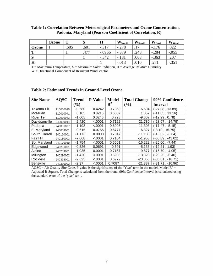
Table 1: Correlation Between Meteorolgical Parameters and Ozone Concentration, Padonia, Maryland (Pearson Coefficient of Correlation, R) Ozone T S H WNorth WSouth WEast WWestOzone 1 .685 .601 -.317 -.278 .17 -.176 .022 T 1 .477 -.0966 -.379 .248 -.284 -.055 S 1 -.542 -.181 .068 -.363 .207 H 1 -.013 .010 .271 -.351 T = Maximum Temperature, S = Maximum Solar Radiation, H = Average Relative Humidity W = Directional Component of Resultant Wind Vector Table 2: Estimated Trends in Ground-Level Ozone Site Name AQSC Trend

(%) P-Value Model

R2Total Change (%)

99% Confidence Interval

Takoma Pk 110010025 -0.680 0.4242 0.7363 -6.594 (-27.08 , 13.89) McMillan 110010041 0.105 0.8216 0.6687 1.057 (-11.05 , 13.16) River Ter 110010043 -1.005 0.0246 0.728 -9.607 (-19.99 , 0.78) Davidsonville 240030014 -2.420 <.0001 0.7122 -21.730 (-28.67 , -14.79) Padonia 240051007 -1.193 <.0001 0.6995 -11.308 (-17.47 , -5.15) E. Maryland 240053001 0.615 0.0755 0.6777 6.327 (-3.10 , 15.75) South Carroll 240130001 -1.173 0.0003 0.7047 -11.130 (-18.62 , -3.64) Fair Hill 240150003 -7.068 <.0001 0.7164 -51.953 (-60.89 , -43.02) So. Maryland 240170010 -1.754 <.0001 0.6661 -16.222 (-25.00 , -7.44) Edgewood 240251001 -0.526 0.0691 0.691 -5.136 (-12.21 , 1.93) Aldino 240259001 -1.035 0.0001 0.7167 -9.877 (-15.70 , -4.05) Millington 240290002 -1.420 <.0001 0.6905 -13.325 (-20.25 , -6.40) Rockville 240313001 -2.625 <.0001 0.6972 -23.356 (-36.01 , -10.71) Beltsville 240330002 -2.37 <.0001 0.7087 -21.337 (-31.71 , -10.96) AQSC = Air Quality Site Code, P-value is the significance of the ‘Year’ term in the model, Model R2 = Adjusted R-Square, Total Change is calculated from the trend, 99% Confidence Interval is calculated using the standard error of the ‘year’ term.

7

Figure 1: Map of Selected Sites

See Figure 2 for reference. The design value site, Edgewood is shown as a star. Beltsville EPA-BEL116 (solar radiation data)

8

Figure 2

R = .685 Figure 3

R = -.317

9

Figure 4

Figure 5

10

Figure 6

11

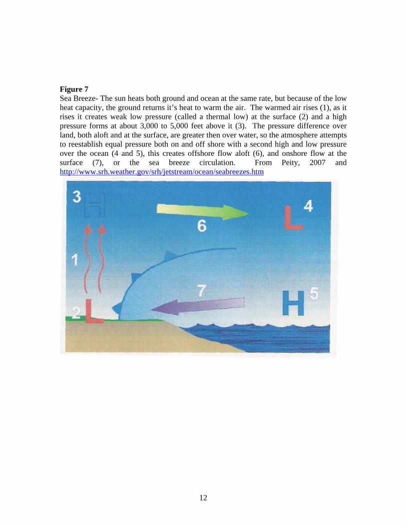
Figure 7 Sea Breeze- The sun heats both ground and ocean at the same rate, but because of the low heat capacity, the ground returns it’s heat to warm the air. The warmed air rises (1), as it rises it creates weak low pressure (called a thermal low) at the surface (2) and a high pressure forms at about 3,000 to 5,000 feet above it (3). The pressure difference over land, both aloft and at the surface, are greater then over water, so the atmosphere attempts to reestablish equal pressure both on and off shore with a second high and low pressure over the ocean (4 and 5), this creates offshore flow aloft (6), and onshore flow at the surface (7), or the sea breeze circulation. From Peity, 2007 and http://www.srh.weather.gov/srh/jetstream/ocean/seabreezes.htm

12

Figure 8 HYSPLIT model results for July 14, 1997

13

Figure 9 HYSPLIT model results for June 26, 2003

14

References Bornstein, R.d., Thunis, P. and Schayes, G., 1993. Simulation of urban barrier effects on polluted urban boundary-layers using the three dimensional URBMET/TVM model with urban topography-new results from New York City. In: Zanetti, P. (Ed.), Air Pollution, Computational Mechanics Publications, Southampton, Boston, 15-34 Boucouvala, D. and Bornstein, R., 2003. Analysis of transport patterns during an SCOS97-NARSTO episode. Atmos. Environ. Vol. 37, #2 S73-S94. Cheng, W. L., 2002. Ozone distribution in coastal central Taiwan under sea-breeze conditions. Atmos. Environ. Vol. 36, 3445-3459 Evtyugina, M., G., Nunes, T., Pio, C. and Costa, C.S., 2006. Photochemical pollution under sea breeze conditions, during summer, at the Portuguese West Coast. Atmos. Environ., Vol. 40, 6277-6293 Gao, F., Sacks J., and Welch, J.W., 1996. Journal of Agricultural, Biological, and Environmental Statistics, Vol. 1, 404-425 Huang, Li-Shan and Smith, Richard L., 1999. Meteorologically-Dependent Trends in Urban Ozone. Environmetrics, Vol. 10, 103-118 Martilli, A., Roulet, Y.A., Junier, M., Kirchner, F., Mathias, W.R. and Clappier, A., 2003. On the impact of urban surface exhange parameterizations on air quality simulations: the Athens case. Atmos. Environ., Vol. 37, 4217-4231 McElroy, M.B. and Smith T.B., 1986. Vertical pollutant distributions and boundary layer structure observed by airborne lidar near the complex California coastline. Atmos. Enivron. Vol. 20, 1555-1566 Milanchus, M.L., Rao, S.T., and Zurbenko, G.Z., 1998. Evaluating the Effectiveness of Ozone Management Efforts in the Presence of Meteorological Variablility. Journal of the Air and Waste Management Association, Vol. 48, 201-215 NRC (National Research Council), 1991. Rethinking the Ozone Problem in Urban and Regional Air Pollution. National Academy Press, Washington. Piety, C., 2007. The Role of Land-Sea Interactions on Ozone Concentrations at the Edgewood, Maryland Monitoring Site. WOE Chapter 6 Porter, P.S., Rao, S.T., Zurbenko, I.G., Dunker, A.M., and Wolff, G.T., 2001. Ozone Air Quality Over North America: Part II—An Analysis of Trend Detection and Attribution Techniques. Journal of the Air and Waste Management Association, Vol. 51, 283-306

15

Rao, S.T. and Zurbenko, I.G., 1994. Detecting and Tracking Changes in Ozone Air Quality. Journal of the Air and Waste Management Association, Vol. 44, 1089-1092 Seaman, N.L. and Michelson, S.A., 1998. Mesoscale meteorological structure of a high-ozone episode during the 1995 NARSTO-Northeast study. J.App. Meto., vol. 39, 384-398. Stull, R.B., 1988. An Introduction to Boundary Layer Meteorology, Springer Publishing, New York, 150-152 Thompson, M.L., Reynolds, J., Cox, L.H., Guttorp, P., and Sampson P.D., 2000. A review of statistical methods for the meteorological adjustment of tropospheric ozone. Atmos. Environ., Vol. 35, 617-630 Zheng, J., Swall, J.L., Cox, W.M., and Davis, J.M., 2006. Interannual variation in meteorologically adjusted ozone levels in the eastern United States: A comparison of two approaches. Atmos. Environ., Vol. 41, 705-716 SAS and all other SAS Institute Inc. product or service names are registered trademarks or trademarks of SAS Institute Inc. in the USA and other countries. ® indicates USA registration. Other brand and product names are registered trademarks or trademarks of their respective companies.

16