Risk-Adjusted Underwriting Performance Measurement

Yingjie Zhang

CNA Insurance Companies

333 South Wabash 30S, Chicago, IL 60604, USA

Email: yingjie.zhang@cna.com

Abstract

To measure economic profits generated by an insurance policy during its

life time, we compare the terminal assets of the policy account with certain

breakeven value. Policies with mutil-year loss payments and income tax pay-

ments are studied. The breakeven value of terminal assets is given in closed

form, and shown to be an increasing function of the claims risk and the asset

investment risk. Profits from underwriting and from capital investment are

measured separately. Simple equations are found that link the cost of capital

to the risk-adjusted loss discount rate. Methods developed in the paper are

also useful for fair premium calculation.

Keywords

Risk-adjusted performance measure, risk-adjusted discount rate, policy-year

profit, cost of capital, EVA, fair premium

1 Introduction

A typical property-casualty insurance policy covers one accident year, but its

claims stay open for many years. The ultimate profitability of the policy cannot

be determined until all claims are settled. In the interim, profits may be estimated

by projecting future investment gains and loss and expense payments. At the

moment the premium is collected, a policy account is established, whose initial

asset is the premium net of acquisition expenses. The value of the asset increases

as investment incomes accumulate, and decreases as losses, expenses and taxes

are paid. At the end of the policy life, the terminal asset of the policy account is

the ultimate profit generated by the policy. A policy is considered profitable, if

its terminal asset exceeds a certain breakeven value. A main goal of the paper is

to calculate this breakeven value.

1

A number of favorable factors allow a policy to generate positive profits. These

include higher premiums collected, lower losses and expenses paid, payments made

later rather than sooner, and extraordinary investment gains. If all these factors

are at their fair or expected values, the resulting terminal asset is the breakeven

terminal asset. Modern finance teaches that the expected return of an asset in-

vestment is in direct proportion to the investment’s risk. Likewise, the breakeven

terminal asset will be shown directly related to the claims risk and the asset in-

vestment risk.

For investment portfolios, there are many risk-adjusted performance measures,

well-known among which are the Sharpe ratio, the Treynor ratio (these are ratio-

based tests), and Jensen’s alpha (this is a value-based test), all thoroughly dis-

cussed in Part 7 of Bodie et al. (2002). In insurance, the risk-adjusted return

on capital (RAROC) and the economic value added (EVA) have become popular.

All these measures, however, are designed for testing performances in one time

period. It is much harder to construct a performance test for a real insurance pol-

icy, whose claim payments span across multiple years. The RAROC and the EVA

are usually applied on the calendar-year basis, thus cannot answer the question

whether a policy (or a policy year) is ultimately profitable.1 The internal rate of

return (IRR) of equity flows is a valid policy-year metric. Yet it cannot be called

a risk-adjusted measure unless it is explicitly linked to the underwriting and in-

vestment risks. Such a link will be discussed in this paper. Further, the RAROC,

IRR and EVA all measure total profits from both underwriting and investment

operations. It is useful for the underwriting managers to know if the underwriting

operation alone, for a particular policy or in a particular year, is successful. Our

approach will address this issue directly.

Few research papers have centered on the economic performance of a multi-

year property-casualty (P&C) policy. Among them Schirmacher and Feldblum

(2006) is a noticeable one. It uses a numerical example to examine how profits

emerge over time. It shows that calendar-year profits depend on accounting sys-

tem. Our concern here is on the ultimate economic profit, which is independent

of the accounting system used. In computing the EVA, Schirmacher and Feld-

blum (2006) assumes that a cost of capital (COC) is given extraneously. As just

mentioned, we will relate it to internal risk metrics.

Profit measurement is intertwined with fair premium determination. The1Some one-year tests have been adapted for use in a multi-year framework and on the policy-

year basis, see Goldfarb (2006). But these are only tentative solutions and lack solid theoretical

support.

2

breakeven level of profit is produced by assuming that the premium is at its

fair level, and investment returns and loss and expense payments are all at their

expected values. Conversely, the fair premium may be determined by setting to

zero the market value of the policy account terminal asset. Our study thus may

be found useful for premium calculation.

The paper is organized as follows. Section 2 starts with a discussion of the risk-

adjusted loss discount rate. The discount rate is used to quantify a policy’s risk.

Then, for a single-year model, the breakeven value of terminal assets is derived.

The breakeven value is an increasing function of asset and claims risks. This result

is generalized to a multi-year model in Section 3. Here a numerical example is

introduced that will be used through out the paper to illustrate calculations. The

main results of the paper are stated in Section 4. Income tax is brought into

the model. Closed-form formulas are derived for the fair premium and breakeven

terminal assets. To obtain tractable results, tax rules are simplified. In Section 5,

we give equations linking the breakeven terminal assets to the COC. A consequence

of the relationship is that the COC is an increasing function of the claims risk,

and a decreasing function of the initial capital. In Section 6, we show how to

define the EVA for the policy account only, and separately measure profits from

underwriting and from capital investment. Section 7 further shows that, since the

loss discount rate and the COC both characterize the internal risk of the company

(assuming investments are risk-free), each can be derived from the other with

simple equations. The fair premium for a policy may be calculated by selecting

either a loss discount rate or a target COC. Section 8 concludes the paper.

2 Benchmark of Underwriting Profit

Issuing an insurance policy establishes a mini-bank, which we will call a policy

account. The starting asset of a policy account is premium minus acquisition

expenses. The value of the asset then changes in time. Investment gains increase

the value, and loss and expense payments decrease it. The remaining assets right

after the last payment is made are called the terminal assets. Actuaries that

have done analysis on finite reinsurance should be familiar with the calculation of

terminal assets. For a policy to be profitable over its lifetime, the terminal assets

must be positive and sufficiently high. Intuitively, the more risky the policy, the

greater the terminal assets need to be. The purpose of this paper is to derive a

benchmark for terminal assets in the framework of modern finance.

3

2.1 Discount Rate for Liabilities

Pricing actuaries use various “loadings” to quantify claims risk of a policy. Load-

ings may be additive or multiplicative, or may be calculated by risk adjusted

discounting. One approach may be easier to apply than another in a given situ-

ation, but they are all equivalent mathematically. The most convenient way for

presenting out results is risk adjusted discounting.

The following example illustrates how the risk adjusted discount rate reflects

the risk level of a policy. Assume a policy has only one loss which will be paid in

one year, and the expected payment is $100. The risk free interest rate is 4%. The

fair premium for the policy is the sum of market values of future claims, expenses,

and capital costs.2 If the claim amount is $100 certain, its market value is the

risk free present value 100/1.04 = 96.15. Market value of a claim increases with

riskiness of the claim, whereas the risk adjusted discount rate decreases. Table 1

shows the risk adjusted rates implied in the market value, with different levels of

claims risk.

Table 1: Risk-Adjusted Discount Rate

risk free Risk-Adjusted

Riskiness Expected Present Discount

of Claim Claim Value Market Value Rate

(1) (2) (3) (4) (5)

No Risk 100.00 96.15 96.15 4%

Low Risk 100.00 96.15 97.09 3%

High Risk 100.00 96.15 200.00 −50%

(5) = (2)/(4)− (1)

In general, let rf be the risk free rate, L the random claim amount, and rl

the claim’s risk adjusted discount rate. Then the risk free present value PV(L) =

E[L]/(1 + rf ), and the market value MV(L) = E[L]/(1 + rl). For a risky claim,

MV(L) > PV(L), the difference being the claim’s risk margin.3 This implies2This fair premium formula is derived from the net present value principle in finance. A well-

known early paper that advocates it is Myers and Cohn (1987). It is now a standard assumption

in theoretical research. Its use in actual pricing is somewhat limited by lack of method for

calculating market value of future claims.3Although it is intuitively clear that if a claim is risky, its value should contain a positive risk

margin, empirical evidence that supports the assertion is sparse. Most authors assume the risk

margin is positive (Myers and Cohn 1987, Bingham 2000). But Feldblum (2006) suggests that

4

rl < rf . If risk is low, rl is close to rf . For a highly risky policy, rl approaches −1.

2.2 Breakeven Terminal Assets

Let p be a policy premium net of acquisition expenses. Then p is the starting

balance of the policy account. Assume the balance is invested in a financial security

whose annual return is a random variable Ra; the policy losses L, paid one year

later, has a risk adjusted discount rate of rl. So the expected return of assets is

ra = E[Ra], and the market value of loss is MV(L) = E[L]/(1 + rl). Capital cost

is not considered in this section.

If the fair premium is charged, then p = MV(L) = E[L]/(1 + rl). At the end

of the year the assets grow to MV(L)(1 +Ra) = E[L](1 +Ra)/(1 + rl). After loss

L is paid, the terminal assets4 are

A1 = MV(L)(1 +Ra)− L

The expected value of terminal assets is

a1 = E[A1] = MV(L)(1 + ra)− E[L] = MV(L)(ra − rl) =E[L]1 + rl

(ra − rl) (2.1)

Since ra ≥ rf and rl ≤ rf , a1 ≥ 0. A more risky security has a greater ra, and a

more risky liability has a smaller rl. So the spread ra − rl is a measure of total

risk of the policy account. a1 is in proportion to the total risk.

a1 is the risk-adjusted breakeven value of terminal assets. If the actual realized

terminal assets are greater than a1, the company makes money on the policy. If the

terminal assets are only slightly positive, but less than a1, the company appears

to make money, but actually does not make enough to compensate for risk. If the

claim or the investment is very risky, the terminal assets need to be very high.

Comparing the actual terminal assets with a1 gives us a value-based test for

underwriting performance. It is interesting to compare this with the combined

ratio, a ratio-based underwriting performance measure. The undiscounted com-

bined ratio is used most often. But it has an obvious shortcoming—it does not

reflect the time value of money. Two lines of business may have the same com-

bined ratio, but the longer tailed line pays out losses more slowly, generates more

investment income along the way, and is more profitable. The economic combined

most P&C liabilities have no systematic risk (i.e., uncorrelated with the market return), thus the

risk margin equals zero. The disagreement can only be settled with future empirical research.4Terminal assets are profits generated by the policy over its lifetime. I choose to use “assets”

rather than “profits” because, for a multi-year model, I will keep track of values of assets from

year to year.

5

ratio (ECR) is introduced to correct this problem. In the calculation of ECR all

underwriting cash flows are discounted, at the risk free rate, to the time of policy

inception. The ECR is strongly advocated in Swiss Re (2006), which claims that

the ECR of 100% “truly indicates the watershed between profit and loss” (page

24). When investments and claims are risky, however, the risk-adjusted breakeven

ECR is not 100%, but something lower. Table 2 gives the breakeven ECR and

the breakeven terminal assets for the three policies in Table 1, with the following

additional assumptions: first, fair premium is charged and there is no expense,

i.e., p = MV(L); and second, investment is riskless, i.e., ra = rf = 4%.

Table 2: Breakeven ECR and Breakeven Terminal Assets

Riskiness Breakeven

of Claim E[L] rl p = MV(L) PV(L) ECR a1

(1) (2) (3) (4) (5) (6) (7)

No Risk 100.00 4% 96.15 96.15 100.0% 0.00

Low Risk 100.00 3% 97.09 96.15 99.0% 0.97

High Risk 100.00 −50% 200.00 96.15 48.1% 108.00

(6) = (5)/(4)

(7) = (4)× (4%− (3))

The ECRs in Table 2 are computed with the fair premium in the denominator.

So they are the breakeven ECRs. The table shows if claims risk is high, the

breakeven ECR is much lower than 100%, and a1 is very large compared to E[L].

3 Multi-Year Underwriting Profit Measure

3.1 Breakeven Terminal Assets an

A typical P&C policy has a multi-year payout pattern. Assume a policy is written

at time 0, and the loss payments are random variables L1, . . . ,Ln, Li paid at time

i. The nominal total loss is L = L1 + . . .+ Ln. We will derive a breakeven value

for terminal assets at time n, after all losses are paid. Assume a loss discount rate

rl, constant throughout the n years, can be found that correctly reflects the risk

of the payments Li’s. Then the market value, at time 0, of the payments is

MV0(L) =E[L1]1 + rl

+ . . .+E[Ln]

(1 + rl)n=

n∑i=1

E[Li](1 + rl)i

(3.1)

6

The fair premium of the policy, net of expenses, equals this market value: p =

MV0(L). Let the premium be invested risk free, and rf be the constant risk free

rate.5 The following formulas give the expected net assets at each time i, after

loss Li is paid

a1 = p(1 + rf )− E[L1]

a2 = p(1 + rf )2 − E[L1](1 + rf )− E[L2]...

...

an = p(1 + rf )n − E[L1](1 + rf )n−1 − . . .− E[Ln]

an is the expected (benchmark) terminal assets of the policy. Substituting equa-

tion (3.1) for p in the last formula, we get

an = (1 + rf )nn∑

i=1

E[Li]((1 + rl)−i − (1 + rf )−i

)(3.2)

= (1 + rf )n (MV0(L)− PV0(L)) (3.3)

MV0(L)− PV0(L) is the risk margin of the policy losses, which is greater than 0

if rl < rf . A less risky policy has a smaller spread rf − rl, and a relatively smaller

an. A very risky policy can have a negative rl, and a very large an.

an is a function of expected values of loss payments, investment rates and

discount rates. These expected values are generally forecasted at the beginning

of the policy term, when an initial an can be computed. an may be revised

later as new information about the claims, markets and general economy comes

in. But it should not be affected by normal fluctuations in loss payments and

investment returns. Final assessment of a policy’s profitability has to wait until

the end of year n, when the actual terminal assets can be calculated. But an

interim estimate may be performed by projecting future actual loss payments and

investment returns. A number of beneficial factors can render a policy profitable:

higher (than expected) premium, smaller losses, slower loss payments, or higher

investment returns. Among them the premium is what a company has the most

control over.

3.2 A Numerical Example

I will use a multi-year numerical example to illustrate the calculations in this

paper. The example is borrowed from Schirmacher and Feldblum (2006), so we5For simplicity, results on multi-year models in this paper are stated for risk free investment

returns. With little additional work, they can be generalized to random (risky) investments, as

long as the investment returns in different time-periods are independent.

7

can compare their methods with ours. Assume a policy is issued on Dec. 31,

20XX, for accident year 20XX+1. The underwriting cash flows are as follows. On

Dec. 31, 20XX (time 0), a premium of $1000 is collected and acquisition expenses

of $275 paid. General expenses of $150 are paid six months later (time 0.5). The

policyholder has one accident in the year and will receice one payment of $650 on

Dec. 31, 20XX+3 (time 3).

Schirmacher and Feldblum (2006) choose a surplus requirement of 25% of the

unearned premium reserve plus 15% of the loss reserve. The risk free rate is 8%

per year compounded semi-annually (4% per half year). The basic policy cash

flows are summerized in Table 3.

Table 3: Policy Account Assets - No Tax

Policy

Investment Account

Time Premium Expense Loss Income Assets

(1) (2) (3) (4) (5) (6)

0.0 1000.00 275.00 0.00 0.00 725.00

0.5 0.00 150.00 0.00 29.00 604.00

1.0 0.00 0.00 0.00 24.16 628.16

1.5 0.00 0.00 0.00 25.13 653.29

2.0 0.00 0.00 0.00 26.13 679.42

2.5 0.00 0.00 0.00 27.18 706.59

3.0 0.00 0.00 650.00 28.26 84.86

Sum 1000.00 425.00 650.00 159.86

PV 1000.00 419.23 513.70

(6)0.0 = (2)0.0 − (3)0.0 − (4)0.0

For i > 0.0, (5)i = (6)i−0.5 × rf

For i > 0.0, (6)i = (6)i−0.5 + (2)i − (3)i − (4)i + (5)i

The nominal losses (L) and expenses (X) add up to $1075, and the premium (p)

is $1000. The underwriting profit is $−75 and the combined ratio is 1075/1000 =

1.075%. The risk free present value of losses and expenses PV0(L+X) = 932.94,

and the ECR equals PV0(L + X)/p = 93.29%. By the ECR standard (Swiss Re

2006, as proposed in) the policy is profitable, but the ECR standard incorrectly

ignores risk.

8

To compute the risk-adjusted breakeven value a3.0, we need a few more as-

sumptions. Assume rl = 3% per half year, and the only loss payment of $650 at

time 3 is both the expected and the actual loss. By (3.2), the breakeven net assets

at time 3 are (1 + 0.04)6 · 650 ·((1 + 0.03)−6 − (1 + 0.04)−6

)= 38.80. Since the

actual terminal assets are $84.86 (column 6 of Table 3, last entry), greater than

$38.80, the policy is profitable under the risk adjusted measure.6

The economic value added by the policy is 84.86 − 38.80 = 46.06. However,

this assessment overstates the quality of the policy, because the $1000 premium

includes a provision for income taxes, but taxes are omitted so far. Taxes are a

significant cost, which I will discuss in the following sections.

4 After-Tax Profit Measures

Insurance companies have a greater tax burden than non-financial companies. In

addition to taxes on profits from underwriting and premium investment, a com-

pany has to pay taxes on gains from capital investment. This cost is dubbed

double taxation—gains from capital investment are taxed twice, first at the cor-

porate level and then at the personal level. All income taxes, including those

from capital investment, should be covered by premium, so that the investor who

contributes capital to the company does not lose out compared with an investor

who directly buys securities on the market. Income taxes are generally a fixed

percentage of the pre-tax income. But the precise IRS tax codes are complex. I

will make simplifying assumptions to obtain closed-form, trackable results.

4.1 Single-year model

Let c be initial capital contributed by shareholders. The capital serves two pur-

poses. First, the company invests the capital to earn income. Second, with the

safety margin provided by the capital, the company is able to issue insurance

policies. Assume the company issues policies and collects premium p (net of ex-

penses), and invests the total cash c + p in securities. The policy loss L is paid

one year later, and the remaining assets are returned to shareholders.

Assume there is one tax rate, denoted by t, for both underwriting and invest-

ment profits. The pretax operating income, from both the policy account and the

capital investment, is (p−L)+(p+ c)Ra = p(1+Ra)−L+ cRa. The total income6In this illustration, for simplicity, I assume that the actual loss payments, investment returns

and discount rates are equal to their expected counterparts. But these two sets of numbers are

usually different.

9

tax, paid at time 1, is t(p(1+Ra)−L)+ tcRa.7 The whole tax payment should be

deducted from the policy account. The policy account’s after-tax net assets are

A1 = p(1 +Ra)− L− t(p(1 +Ra)− L)− tcRa

= (1− t)(p(1 +Ra)− L− tc

1− tRa

)(4.1)

Policy premium p is considered fair if it makes the market value of terminal assets

zero. Setting MV(A1) = 0, and noting MV(1+Ra) = 1 and MV(Ra) = rf/(1+rf ),

we have

p = MV(L) +tcrf

(1− t)(1 + rf )(4.2)

The second term is the amount of premium needed to cover taxes on investment

income of capital, which is in direct proportion to c. So too much capital hurts the

company in price competition. Also note that the fair premium is not affected by

how the premium and capital are invested. To derive the expected terminal assets

for the policy, we substitute (4.2) into (4.1), and calculate the expected values

a1 = (1− t)((

MV(L) +tcrf

(1− t)(1 + rf )

)(1 + E[Ra])− E[L]

)− tcE[Ra]

= (1− t)MV(L)(ra − rl)−tc

1 + rf(ra − rf )

= (1− t)E[L]1 + rl

(ra − rl)−tc

1 + rf(ra − rf ) (4.3)

This is the risk-adjusted breakeven value for the after-tax terminal assets. In (4.3)

the first term is essentially the after-tax version of the breakeven value (2.1), and

the second term reflects tax on capital. A policy generates a profit if and only if

its after-tax terminal assets are greater than a1.

Consider a special case where the investment is risk free, i.e., ra = rf . Formula

(4.3) reduces to

a1 = (1− t)E[L]1 + rl

(rf − rl) (4.4)

Remember rl ≤ rf , and the riskier the policy, the smaller the rl. So a riskier

policy has a greater breakeven value (4.4). Note that capital c does not appear in

(4.4). This is because, as the investment is risk free, the amount of tax on capital

gain is certain, and is exactly covered by the second component of fair premium

(4.2).7In practice, when taxable income is negative, the company may not be able to receive full

tax refund in the current year. But we will ignore this complication here.

10

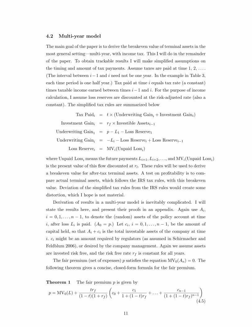
4.2 Multi-year model

The main goal of the paper is to derive the breakeven value of terminal assets in the

most general setting—multi-year, with income tax. This I will do in the remainder

of the paper. To obtain trackable results I will make simplified assumptions on

the timing and amount of tax payments. Assume taxes are paid at time 1, 2, . . . .

(The interval between i−1 and i need not be one year. In the example in Table 3,

each time period is one half year.) Tax paid at time i equals tax rate (a constant)

times taxable income earned between times i−1 and i. For the purpose of income

calculation, I assume loss reserves are discounted at the risk-adjusted rate (also a

constant). The simplified tax rules are summarized below

Tax Paidi = t× (Underwriting Gaini + Investment Gaini)

Investment Gaini = rf × Investible Assetsi−1

Underwriting Gain1 = p− L1 − Loss Reserve1

Underwriting Gaini = −Li − Loss Reservei + Loss Reservei−1

Loss Reservei = MVi(Unpaid Lossi)

where Unpaid Lossi means the future payments Li+1, Li+2, . . ., and MVi(Unpaid Lossi)

is the present value of this flow discounted at rl. These rules will be used to derive

a breakeven value for after-tax terminal assets. A test on profitability is to com-

pare actual terminal assets, which follows the IRS tax rules, with this breakeven

value. Deviation of the simplified tax rules from the IRS rules would create some

distortion, which I hope is not material.

Derivation of results in a multi-year model is inevitably complicated. I will

state the results here, and present their proofs in an appendix. Again use Ai,

i = 0, 1, . . . , n − 1, to denote the (random) assets of the policy account at time

i, after loss Li is paid. (A0 = p.) Let ci, i = 0, 1, . . . , n − 1, be the amount of

capital held, so that Ai + ci is the total investable assets of the company at time

i. ci might be an amount required by regulators (as assumed in Schirmacher and

Feldblum 2006), or desired by the company management. Again we assume assets

are invested risk free, and the risk free rate rf is constant for all years.

The fair premium (net of expenses) p satisfies the equation MV0(An) = 0. The

following theorem gives a concise, closed-form formula for the fair premium.

Theorem 1 The fair premium p is given by

p = MV0(L) +trf

(1− t)(1 + rf )

(c0 +

c11 + (1− t)rf

+ . . .+cn−1

(1 + (1− t)rf )n−1

)(4.5)

11

Premium calculation will be discussed in depth in Section 7. To derive the

breakeven value for the after-tax terminal assets, we start from time 0 with pre-

mium (4.5), and successively compute underwriting, investment, tax cash flows,

and the net policy account assets Ai. The result is also a simple closed-form for-

mula.

Theorem 2 The breakeven value for the after-tax terminal assets in the policy

account is given by

an =(1− t)(rf − rl)(1 + (1− t)rf )n

(1− t)rf − rl

n∑i=1

E[Li](

1(1 + rl)i

− 1(1 + (1− t)rf )i

)=

(1− t)(rf − rl)(1 + (1− t)rf )n

(1− t)rf − rl(MV0(L)− PVtax

0 (L)) (4.6)

where PVtax0 (L) stands for the present value discounted with the after-tax interest

rate (1− t)rf .

Formula (4.6) does not involve taxes on capital investments (ci’s do not appear

in the formula). This is because the tax component in fair premium (4.5) exactly

covers all those taxes. (As in the single-year model, if investments are risky, the

breakeven terminal assets will depend on the ci’s.)

These formulas are easy to apply. In Table 4, a tax column is added to Ta-

ble 3, and the policy account assets at each time are recalculated by deducting

taxes. (Note that the tax column contains all taxes, including that on capital

investments.) The last entry of column 7 gives the policy’s after-tax terminal

assets of $33.55. Given the rates rf = 4%, rl = 3% and t = 35%, we compute

MV0(L) = 650/(1+0.03)6 = 544.36, and PVtax0 (L) = 650/(1+(1−0.35)×0.04)6 =

557.22. Substituting these figures into (4.6), we get the breakeven terminal assets

a3.0 = 24.37. Since this is less than the actual terminal assets of $33.55, the policy

is profitable. The value added by the policy is 33.55− 24.37 = 9.18.

Calculation of the breakeven value an, formula (4.6), does not require the

values of ci. But ci’s are needed in the fair premium formula (4.5).

5 Linking Breakeven Terminal Assets to Cost of Cap-

ital

The cost of capital (COC) is the rate of return on capital required by shareholders.

Shareholder return is a random variable, and the COC is the expected value of

this return. According to modern finance, the COC is in direct proportion to

the riskiness of the return. For the insurance models under consideration, risk of

12

Table 4: Policy Account Assets - After Tax

Policy

Investment Account

Time Premium Expense Loss Tax Income Assets

(1) (2) (3) (4) (5) (6) (7)

0.0 1000.00 275.00 0.00 -26.25 0.00 751.25

0.5 0.00 150.00 0.00 32.45 30.05 598.86

1.0 0.00 0.00 0.00 29.39 23.95 593.42

1.5 0.00 0.00 0.00 8.13 23.74 609.03

2.0 0.00 0.00 0.00 7.97 24.36 625.43

2.5 0.00 0.00 0.00 -3.57 25.02 654.01

3.0 0.00 0.00 650.00 -3.38 26.16 33.55

Sum 1000.00 425.00 650.00 44.73 153.28

PV 1000.00 419.23 513.70 40.55

Column (5) from Table 2 in Schirmacher and Feldblum (2006).

(7)0.0 = (2)0.0 − (3)0.0 − (4)0.0 − (5)0.0

For i > 0.0, (6)i = (7)i−0.5 × rf

For i > 0.0, (7)i = (7)i−0.5 + (2)i − (3)i − (4)i − (5)i + (6)i

the shareholder return comes from two sources—volatilities in investment gains

and claim payments. In the preceeding sections, I have shown that the expected

values of claims and investment gains determine an expected value of terminal

assets in the policy account. The total return to shareholders is the sum of policy

account terminal assets and the investment return on capital. Therefore, the COC

is a simple function of the breakeven terminal assets and the expected investment

return on capital. This relationship may also be used reversly: if the COC is

obtained through stock analysis, a required level of terminal assets can be inferred,

which may lead to useful premium calculation.

5.1 Single-year model

The expected value of policy account terminal assets is given in equation (4.3).

The expected value of capital investment at time 1 is c(1 + ra). Therefore, the

13

total expected after-tax net assets at time 1 are

(1− t)MV(L)(ra − rl)−tc

1 + rf(ra − rf ) + c(1 + ra) (5.1)

The expected rate of return on capital is

COC =(1− t)MV(L)

c(ra − rl)−

t

1 + rf(ra − rf ) + ra (5.2)

By (5.2), the COC is the sum of three terms: the investment rate of return ra; the

after-tax spread (1− t)(ra − rl) times the “leverage ratio” MV(L)/c; and a term

related to taxes on capital investment, which vanishes if the investment is risk free.

The following factors would cause the COC to increase (i.e., shareholders require

a greater return): riskier investments (greater ra), more volatile claims (smaller

rl), or a higher leverage ratio. Increasing the amount of capital would reduce the

COC.

In Appendix 2, I will explain that formula (5.2) is consistent with the CAPM.

In the CAPM world, an asset’s expected return is in direct proportion to its β,

which is a measure of the asset’s systematic risk. I will use the given asset rate

ra and liability rate rl to determine β of the shareholder return, and show the

expected value of the return—the COC—is exactly given by (5.2).

5.2 Multi-year model

In a multi-year model, shareholders contribute an initial capital c0 and establish a

capital account. The capital account then earns investment income and pays out

dividends (releases capital). Let ci be the amount of capital held at time i. Then

the total assets at time i are Ai + ci.8 Assume the interim dividends are released

entirely from the capital account; the policy account only distributes its profit

at time n.9 Therefore, the dividend at time i is simply ci−1 plus the investment

income in the year minus ci. If each ci is invested at the constant risk free rate

rf , then the divident flows out of the capital account are −c0, c0(1 + rf ) − c1,

c1(1 + rf )− c2, . . . , cn−1(1 + rf ). Obviously, the internal rate of return (IRR) of

these flows is rf .

The expected terminal assets an of the policy account is given in (4.6). Thus

the expected total dividend flows are −c0, c0(1 + rf ) − c1, c1(1 + rf ) − c2, . . . ,

8The asset in this paper corresponds to the income-producing asset in Schirmacher and Feld-

blum (2006). Non-income-producing assets, like the DTA, are not considered.9This distinction between the policy account and the capital account does not affect profit

measurement of the company as a whole. But it is important for measuring the policy account

profit separately from the capital account.

14

cn−1(1 + rf ) + an. The IRR of the total dividend flows is given by the following

equation

c0 =c0(1 + rf )− c1

1 + IRR+c1(1 + rf )− c2

(1 + IRR)2+ . . .+

cn−1(1 + rf ) + an

(1 + IRR)n(5.3)

This IRR is the average—over n years—cost of capital of the company. After a

policy has run its course, we can compute the IRR of the actual capital flows. If

the IRR is greater than (less than) the average COC given by (5.3), the company’s

overall operation is profitable (unprofitable). It is worth noting that, since an > 0,

the COC is greater than the expected asset rate of return. A greater claims risk

implies a greater spread rf − rl, thus a greater an and a greater COC.

Back to the example of Table 4. In their paper, Schirmacher and Feldblum

(2006) assume the required capital is 25% of the unearned premium reserve plus

15% of the loss reserve. They then compute the required assets at each time i

and the corresponding dividend flows. Table 5 shows the dividend flows out of the

capital account (column 6), the total dividend flows (column 7), and the breakeven

flows (column 8). These three columns only differ in their last entry. The IRR for

column 6 equals the asset rate of return 4%, as expected. The IRR for column 7

is 6.18% (obtained also in Schirmacher and Feldblum 2006). The IRR for column

8, 5.62%, is the COC. Since the IRR of total dividend flows is greater than the

COC, the company creates value for shareholders.

6 Decomposing the EVA

Shareholders invest captal in a company expecting to earn the cost of capital. If

they earn more than (less than) the COC, then the investment adds (destroys)

value. The economic value added is defined as (see, e.g., Schirmacher and Feldblum

2006)

EVA = After-tax Net Income− COC× Capital Held

The second term in the formula, COC × Capital Held is the breakeven value of

after-tax income. So this scheme of measuring profits is similar to what we de-

veloped in sections 2 to 4. The difference is that, the EVA measures the total

profits, while our method addresses profitability of the policy account. From our

discussion so far, it is straightforward to decompose this EVA measurement into

one for the policy account and another for the capital account.

15

Table 5: Dividend Flows

Capital

Policy Investment Account Total Breakeven

Account Capital Total Income on Dividend Dividend Dividend

Time Assets Held Assets Capital Flow Flow Flow

(1) (2) (3) (4) (5) (6) (7) (8)

0.0 751.25 428.75 1180.00 0.00 -428.75 -428.75 -428.75

0.5 598.86 362.62 961.48 17.15 83.28 83.28 83.28

1.0 593.42 149.53 742.95 14.50 227.60 227.60 227.60

1.5 609.03 122.54 731.58 5.98 32.97 32.97 32.97

2.0 625.43 94.77 720.20 4.90 32.67 32.67 32.67

2.5 654.01 79.84 733.85 3.79 18.73 18.73 18.73

3.0 33.55 0.00 33.55 3.19 83.03 116.58 107.40

IRR 4.00% 6.18% 5.62%

Column (2) is column (7) in Table 4.

Column (4) from Table 7 in Schirmacher and Feldblum (2006).

For i > 0.0, (5)i = (3)i−0.5 × rf

For i > 0.0, (6)i = (2)i−0.5 + (5)i − (2)i

For i < 3.0, (7)i = (6)i; (7)3.0 = (6)3.0 + (7)3.0 in Table 4

For i < 3.0, (8)i = (6)i; (8)3.0 = (6)3.0 + a3.0 (a3.0 calculated in Section 4.2)

6.1 Single-year model

For the single-year model, the COC is given in formula (5.2), which can be split

into two parts. The last term, ra, is the hurdle rate for the capital account. If the

actual return on capital is greater than ra, then the investment operation adds

value. By Section 4.1, the first two terms of (5.2) gives the hurdle rate of the

policy account. This leads to the following definition of EVA for the two accounts

separately

EVAc = c× (Actual Investment Rate− ra) (6.1)

EVAp = Actual After-tax terminal assets

−(1− t)MV(L)(ra − rl) +tc

1 + rf(ra − rf ) (6.2)

16

In (6.2) the actual assets in the policy account are after all taxes, including those

on capital gains. Readers familiar with investment portfolio analysis may recognize

that the rate spread, Actual Investment Rate − ra, in (6.1) is Jensen’s alpha for

the asset portfolio. Obviously, EVA = EVAc + EVAp. If one wish to review the

past underwriting performance and make price change, EVAp would provide more

accurate information than the EVA.

There are previous efforts on finding methods to separately measure under-

writing and investment activities. Bingham (2004) proposes to allocate capital

between underwriting and asset investment, find a cost of capital for each of the

functions, and separately calculate their value creation. In practice, some compa-

nies build models to calculate the underwriting ROE, the investment ROE, and

ROEs at various policy group or investment portfolio levels. Our method has some

unique features. First, it emphasizes that income tax on capital investment should

be deducted from policy account profits. Second, it treats the capital account no

different than other investment portfolios, and test it with the established Jensen’s

alpha. Third, it is consistent with the CAPM (see Appendix 2), so is theoretically

solid.

The policy account itself consists of two activities, underwriting (collecting

premiums and paying losses) and investment of premium. But these two activities

are more intertwined and we cannot measure them separately. An increase in

premium is an achievement of the underwriting department. The resulting gain

in profit should be credited entirely to underwriting, not to investment. But the

additional premium generates an additional investment income, which cannot be

cleanly attributed to either underwriting or investment. Also, the policy account

covers income tax on capital investments. It is not clear whether this tax should

be covered by underwriting profits or by investment income. Even in our method,

performances of the capital account and the policy account are not completely

independent. If capital investment generates a higher return, the corresponding

income tax increases, which reduces EVAp.

6.2 Multi-year model

In general, the EVA is calculated annually based on that year’s income. For an n-

year model, this means a stream of n EVAs that depends on how loss reserves are

set in a particular accounting system. Schirmacher and Feldblum (2006) compute

the EVA stream in two accounting systems, the NPV and the IRR. I will not deal

with accounting rules here, but only discuss the measurement of economic profits

at the end of the policy life.

17

The IRR of the total dividend flows, denoted by IRRtot, is a standard profit

measure of shareholders’ investment. The cost of capital is the breakeven value

of IRRtot. As shown in Section 5.2, the total dividend flows are the sum of two

component flows: a single flow at time n—the terminal assets—from the policy

account, and a stream of dividends from the capital account. Methods of evalu-

ating the two component flows have essentially been derived in previous sections,

which are summarized below.

For the policy account, we define

EVAp = Actual After-tax terminal assets− an (6.3)

EVAp is the ultimate cash value added by the policy. For the example in Table

5, EVAp = 33.55− 24.37 = 9.18. The dividend flows out of the capital account is

most conveniently measured by the IRR, denoted by IRRc. The breakeven value

of IRRc is the expected investment return ra (or rf , if capitals are invested risk

free). Clearly, if EVAp > 0 and IRRc > ra, then IRRtot > COC; conversely, if

EVAp < 0 and IRRc < ra, then IRRtot < COC. Note that EVAp, IRRc and IRRtot

are all independent of accounting system. EVAp provides more useful information

to underwriting management than IRRtot.

Here is an extreme situation that in a profitable company the underwriting

operation is very unprofitable. An unexpected large loss may exhaust policy ac-

count assets before claims are settled. That is, Ai ≤ 0 for some i < n. When this

happens, the policy account assets stay negative for all later years. The negative

EVAp would correctly indicate that the policy is unprofitable. However, if the

capital investment generates large returns, it is possible that IRRtot still exceeds

the COC, indicating a profitable overall operation. IRRtot here says nothing about

the underwriting performance.

7 Comparing Direct and Indirect Pricing Methods

Insurance pricing methods are broadly divided into two types. The direct methods

are represented by Myers and Cohn (1987), formula (3.4). In these methods, risk

of future claims is quantified by the risk load—in this paper, the risk adjusted

discount rate. With an indirect method, a target return on capital is first chosen,

which is to match the total risk of claims and investments. Then the premium

is back-solved to achieve this target. If both methods produce the same fair

premium, they are economically equivalent. The formulas derived in sections 4

and 5 give us a mathematical relationship between the two methods.

18

Formula (4.5) is a direct method for computing p. rl is the key parameter that

captures the risk of claims.10 A corresponding indirect method works via these

steps: choose a COC, substitute it into (5.3) to get an, solve (4.6) (using a nu-

merical method like Goal Seek or Solver in Excel) for rl, and then compute p with

(4.5). This also shows how rl and the COC, the two variables that characterize

risk, uniquely determine each other.

I will demonstrate these calculations with the same example. In Section 4.2,

we selected rl = 3% and calculated MV0(L) = 544.36. Substituting this MV0(L)

and the ci’s in column 3 of Table 5 into (4.5), yields p = 569.08. Loading in

the present value of expenses, $419.23, we get the full policy premium of $988.31.

(This breakeven value is less than the actual charge of $1000. Thus the policy is a

good deal to beginning with.) To illustrate the algorithm from the COC to rl and

p, we adopt the assumption in Schirmacher and Feldblum (2006) that the COC

is 5%. Plugging this IRR into the denominators of (5.3), and the ci’s in column 3

of Table 5 into the numerators, we obtain an = $14.76. Now use equation (4.6).

Since there is only one loss payment of $650 at time 3, MV0(L) = 650/(1 + rl)6,

where rl is an unknown variable. Also PVtax0 (L) = 557.22. Plugging these and

all known parameters into (4.6) and solving for rl, we have rl = 3.39%. Using

this rl in (4.5) gives p = 556.98. Adding in $419.23 for expenses we obtain the

total policy premium of $976.21. To sum up, rl = 3% corresponds to a COC of

5.62% (column 8 of Table 5), and rl = 3.39% corresponds to a COC of 5%; the

first scenario is more risky, and has a higher premium of $988.31 (vs. $976.21 for

the second scenario.)

To use these approaches in a pricing project, it is imperative to determine

the capitals (required or desired) c0, c1, . . . , cn−1. In a multi-line company, the

company-wide capital needs to be allocated at each time i. More research is needed

on these issues.

8 Conclusions

In this paper, we studied risk-adjusted performance measures. We focused on the

measurement of terminal assets of the policy account. By comparing the terminal

asset with a breakeven value, we determine the the amount of profit created by

the policy over its lifetime. The main results of the paper are the two theorems

in Section 4.2, in which the breakeven terminal asset is formulated in closed form10Although we have been addressing calculating MV0(L) with the risk adjusted discount rate,

formula (4.5) would still apply if MV0(L) can be obtained with another method.

19

in terms of the rates of investment return and loss discounting. In contrast to

the familiar risk-adjusted performance measures, the RAROC and the EVA, our

approach addresses the underwriting profits separately from capital investment

results. The mathematical relationship between the terminal asset, the cost of

capital and the EVA is also discussed.

A key input for calculating the fair premium and the breakeven terminal as-

sets, formulas (4.5) and (4.6), is the loss discount rate rl. It characterizes the

underwriting risk of the policy. A link between rl and the COC, which reflects

the total risk of the company, is discussed in Section 7. How to select either rlor the COC to correctly reflect risk is a challange in application of the formulas.

Determination of the stream of capitals ci also needs further research.

20

References

Bingham, R. E. (2000). The Direct Determination of Risk-Adjusted Discount

Rates and Liability Beta. Proceedings of the Casualty Actuarial Society,

LXXXVII:1–30.

Bingham, R. E. (2004). Value Creation in Insurance - A Finance Perspective.

Proceedings of the Casualty Actuarial Society, XCI:85–117.

Bodie, Z., Kane, A., and Marcus, A. (2002). Investments. McGraw-Hill/Irwin.

Feldblum, S. (2006). Fair Value Accounting for Property-Casualty In-

surance Liabilities. In 2006 Discussion Paper Program - Current Is-

sues in Insurance Financial Statements, pages 1–35. Available online

http://www.casact.org/pubs/dpp/dpp06/.

Goldfarb, R. (2006). Risk-Adjusted Performance Measurement for P&C In-

surers. Study notes for CAS Exam 9. Download at the CAS website

http://www.casact.org/library/studynotes/goldfarb8.2.pdf.

Myers, S. S. and Cohn, R. A. (1987). A Discounted Cash Flow Approach to

Property-Liability Insurance Rate Regulation. In Cummins, J. D. and Harring-

ton, S. E., editors, Fair Rates of Return in Property-Liability Insurance, pages

55–77. Dordrecht: Kluwer Nijhoff Publishing.

Schirmacher, E. and Feldblum, S. (2006). Financial Pricing Models for Property-

Casualty Insurance Products: Retrospective Analysis. North American Actu-

arial Journal, 10(2):1–27.

Sherris, M. (2003). Economic Valuation: Something Old, Something New. Aus-

tralian Actuarial Journal, 9(4):625–665.

Swiss Re (2006). Measuring Underwriting Profitability of the Non-Life Insurance

Industry. Swiss Re Sigma, No3/2006.

Appendix 1. Proof of the Theorems

Proof of Theorem 1

Formula (4.5) can be written as

p =n∑

i=1

(MV0(Li) +

trfci−1

(1− t)(1 + rf )(1 + (1− t)rf )i−1

)(8.1)

21

We only need to prove the theorem for each i, that is, for a policy with a single

loss payment Li at time i, and with a single nonzero capital ci−1 at time i − 1

(considered beginning of year i), the fair premium is given by

p = MV0(Li) +trfci−1

(1− t)(1 + rf )(1 + (1− t)rf )i−1(8.2)

If (8.2) holds for all i, then (8.1) is true simply by additivity.

If time i is the only time losses and capital account taxes are paid, then at all

other times j, j = 1, . . . i − 1, i + 1, . . . n, the only payments are taxes on policy

account profits. These profits need to be carefully calculated according to the

rules stated in Section 4.2.

Let MVj(Li) be the market value of Li at time j < i. The value of MVj(Li)

will not be known until time j. Therefore, viewed at time 0, MVj(Li) is a random

variable.11. To simplify notations, let MVj(Li) be denoted by Vj . The loss reserve

at time j < i is Vj , and loss reserves are zero after time i. In the following

derivation, I start by calculating the net assets at time 1, move forward in time,

and end up with terminal assets at time n. I then set the market value of the

terminal assets to zero, and solve for the fair premium p.

At time 1, the underwriting gain is p−V1 and the investment gain is prf . Then

the tax is t(p(1 + rf )− V1). The net assets at time 1 are

A1 = p(1 + rf )− t(p(1 + rf )− V1) = p(1 + rf )(1− t) + tV1

At time 2, the underwriting gain is V1 − V2 and the investment gain is A1rf .

Then the tax is t(V1 − V2 +A1rf ). The net assets at time 2 are

A2 = A1(1 + rf )− t(V1 − V2 +A1rf )

= p(1 + rf )(1− t)(1 + (1− t)rf ) + tV2 + rf t(1− t)V1

In general, the tax at any time j < i is t(Vj−1−Vj +Aj−1rf ), and it is not hard

to prove by induction that the net assets at j is given by the following formula

Aj = p(1 + rf )(1− t)(1 + (1− t)rf )j−1 + tVj + rf t(1− t)(Vj−1

+(1 + (1− t)rf )Vj−2 + . . .+ (1 + (1− t)rf )j−2V1

)(8.3)

Now this formula holds for Ai−1. At time i, there are two additional payments,

loss Li and tax on capital investment trfci−1, and no further loss reserves. So the

11Rigorously, the market values MV0(Li), MV1(Li), . . . , MVi−1(Li), Li, are a stochastic

process adapted to a filtration indexed by time j.

22

total tax is t(Vi−1 − Li +Ai−1rf ) + trfci−1, and the net assets are

Ai = Ai−1(1 + rf )− t(Vi−1 − Li +Ai−1rf )− trfci−1

= p(1 + rf )(1− t)(1 + (1− t)rf )i−1 − (1− t)Li + rf t(1− t)(Vi−1

+(1 + (1− t)rf )Vi−2 + . . .+ (1 + (1− t)rf )i−2V1

)− rf tci−1 (8.4)

After time i, every year the assets Ai are reinvested and taxes on the investment

gains paid. The after-tax investment rate of return is (1− t)rf . So, the terminal

assets at time n are

An = Ai(1 + (1− t)rf )n−i (8.5)

The fair premium p is so defined as to make the market value of An zero. By

(8.5), MV0(An) = 0 if and only if MV0(Ai) = 0. So we need to calculate the

market value of each term in (8.4).

The first and the last term in (8.4) are nonrandom constants. The market

value, at time 0, of a constant is the constant divided by (1 + rf )i. The market

values of other terms in (8.4) are obtained using the following formula.

MV0(Vj) = MV0(Li)/(1 + rf )i−j (8.6)

I will use this formula now to complete the proof. The formula itself will be proved

later in the section.

MV0(Ai)

= MV0(p(1 + rf )(1− t)(1 + (1− t)rf )i−1)− (1− t)MV0(Li) + rf t(1− t)(

MV0(Vi−1)

+(1 + (1− t)rf )MV0(Vi−2) + . . .+ (1 + (1− t)rf )i−2MV0(V1))−MV0(rf tci−1)

=p(1− t)(1 + (1− t)rf )i−1

(1 + rf )i−1− (1− t)MV0(Li)

+rf t(1− t)

1 + rfMV0(Li)

(1 +

1 + (1− t)rf1 + rf

+ . . .+(1 + (1− t)rf )i−2

(1 + rf )i−2

)−

rf tci−1

(1 + rf )i

=p(1− t)(1 + (1− t)rf )i−1

(1 + rf )i−1− (1− t)MV0(Li)

+rf t(1− t)

1 + rfMV0(Li)

(1−

(1 + (1− t)rf )i−1

(1 + rf )i−1

)÷(

1−1 + (1− t)rf

1 + rf

)−

rf tci−1

(1 + rf )i

=p(1− t)(1 + (1− t)rf )i−1

(1 + rf )i−1−

(1− t)(1 + (1− t)rf )i−1

(1 + rf )i−1MV0(Li)−

rf tci−1

(1 + rf )i

Setting MV0(Ai) = 0 and solving for p, we get the formula (8.2). This proves

Theorem 1.

23

Note that in the derivation of (4.5) we do not need the assumption that there is

a constant risk-adjusted discount rate rl. Therefore, (4.5) can be used to calculate

the fair premium whenever the market value MV0(L) can be reasonably estimated.

Proof of formula (8.6)

In formula (8.4), Ai is a random variable conditioned on all information up to

time i. This conditioning statement is important when computing the market

value of Vj . Vj = MVj(Li) is a random variable viewed at any point j′ < j, but is

nonrandom at any j′ > j. So it is easy to first discount Vj to time j,

MVj(Vj) = Vj/(1 + rf )i−j

Then, further discounting the above to time 0, we get

MV0(Vj) = MV0(MVj(Li))/(1 + rf )i−j = MV0(Li)/(1 + rf )i−j

which proves (8.6).12

Proof of Theorem 2

Theorem 2 says if a policy charges premium (4.5), then its expected terminal assets

at time n have the form (4.6). I will again prove the theorem by splitting it into

n simpler components. For any i < n, assume that a sub-policy i has premium

(8.2), makes only one loss payment Li at time i, and is supported by one nonzero

capital ci−1 at time i − 1. I will prove that the expected terminal assets of the

sub-policy, at time n, are given by the following formula

an,i =(1− t)(rf − rl)(1 + (1− t)rf )n

(1− t)rf − rlE[Li]

(1

(1 + rl)i− 1

(1 + (1− t)rf )i

)(8.7)

Obviously, the expected terminal assets of the original policy is the sum of these

an,i’s. This will prove Theorem 2.

Substituting (8.2) into the righthand side of (8.4), we have

Ai =(V0 +

trfci−1

(1− t)(1 + rf )(1 + (1− t)rf )i−1

)×(1 + rf )(1− t)(1 + (1− t)rf )i−1 − (1− t)Li

+rf t(1− t)(Vi−1 + (1 + (1− t)rf )Vi−2 + . . .+ (1 + (1− t)rf )i−2V1

)− rf tci−1

12A rigorous proof of the formula may be stated with stochastic discount factors. The technique

is standard in asset pricing theory.

24

The assumption that there is a constant loss discount rate rl implies that E[Vj ] =

E[Li]/(1 + rl)i−j . Noting that the ci−1 terms cancel out, we have

E[Ai] = (1 + rf )(1− t)(1 + (1− t)rf )i−1 E[Li](1 + rl)i

− (1− t)E[Li]

+rf t(1− t)

1 + rlE[Li]

(1 +

1 + (1− t)rf1 + rl

+ . . .+(1 + (1− t)rf )i−2

(1 + rl)i−2

)= (1 + rf )(1− t)(1 + (1− t)rf )i−1 E[Li]

(1 + rl)i− (1− t)E[Li]

+rf t(1− t)

1 + rlE[Li]

(1−

(1 + (1− t)rf )i−1

(1 + rl)i−1

)÷(

1−1 + (1− t)rf

1 + rl

)= (1 + rf )(1− t)(1 + (1− t)rf )i−1 E[Li]

(1 + rl)i− (1− t)E[Li]

+rf t(1− t)

rl − (1− t)rfE[Li]

(1−

(1 + (1− t)rf )i−1

(1 + rl)i−1

)=

((1 + rf )(1− t)(1 + (1− t)rf )i−1 E[Li]

(1 + rl)i−

rf t(1− t)rl − (1− t)rf

E[Li](1 + (1− t)rf )i−1

(1 + rl)i−1

)+(−(1− t)E[Li] +

rf t(1− t)rl − (1− t)rf

E[Li])

=(1− t)(rf − rl)(1 + (1− t)rf )i

(1− t)rf − rl

E[Li](1 + rl)i

−(1− t)(rf − rl)(1− t)rf − rl

E[Li]

Ai is the net asset at time i. After time i, the asset grows at the after-tax

investment yield (1− t)rf . So the terminal net assets at time n is An,i = Ai(1 +

(1− t)rf )n−i. Therefore,

an,i = E[An,i] = E[Ai](1 + (1− t)rf )n−i

=(1− t)(rf − rl)(1 + (1− t)rf )n

(1− t)rf − rlE[Li]

(1

(1 + rl)i− 1

(1 + (1− t)rf )i

)This proves (8.7), thus completes the proof of Theorem 2.

Appendix 2. Formula (5.2) is Consistent with the CAPM

Assume our insurance company exists in a CAPM world. That is, the invested

assets, the claims and the shareholders’ capital all satisfy the CAPM. For the

invested assets we have

E[Ra] = ra, ra − rf = βam (8.8)

where m is the market risk premium. For a policy with premium p (net of ex-

penses) and future claim L, we define its “return” to be Rl = (L − p)/p, and

assume that

E[Rl] = rl, rl − rf = βlm (8.9)

25

This liability CAPM is a natural extension of the standard (investment) CAPM,

and has been proposed by many authors, see, for example, Sherris (2003). rl ≤ rf

implies βl ≤ 0. An implicit assumption in this CAPM framework is that all assets

are traded at the market value, and all policies are charged the fair premium,

which equals the market value of claims.

Formula (4.2) provides a policy’s fair premium p. Substituting it into formula

(4.1) gives the after-tax policy account net assets at time 1. Adding in the value

of the capital amount we have the following total net assets

C ≡ (1− t)MV(L)(Ra −Rl)−tc

1 + rf(Ra − rf ) + c(1 +Ra) (8.10)

The return on capital, Rc = (C − c)/c, is

Rc =(1− t)MV(L)

c(Ra −Rl)−

t

1 + rf(Ra − rf ) +Ra

=(

1 +(1− t)MV(L)

c− t

1 + rf

)Ra −

(1− t)MV(L)c

Rl

+t

1 + rfrf (8.11)

Based on formula (8.11), the shareholder investment C can be replicated by the

following three investments: short-selling an asset, whose return is Rl, and receiv-

ing cash (1− t)MV(L); lending an amount tc/(1 + rf ) at the risk free rate rf ; and

buying an asset, whose return is Ra, with the net cash c+(1−t)MV(L)−tc/(1+rf ).

Thus, the β of the investment C is given by the weighted average of β’s of the

three investments

βc =(

1 +(1− t)MV(L)

c− t

1 + rf

)βa −

(1− t)MV(L)c

βl (8.12)

If C satisfies the CAPM, then E[Rc]− rf = βcm. Using (8.8) and (8.9), we obtain

E[Rc] =(

1 +(1− t)MV(L)

c− t

1 + rf

)ra −

(1− t)MV(L)c

rl +t

1 + rfrf

= ra +(1− t)MV(L)

c(ra − rl)−

t

1 + rf(ra − rf ) (8.13)

This is exactly the COC in formula (5.2).

26