market power without strategic behavior (monopoly or monopolistic competition)
TRANSCRIPT

Market Power
Without Strategic Behavior(Monopoly or Monopolistic Competition)

Monopoly• Firm with monopoly or market power has
the ability to set its price and produce at any point on the market demand curve
• Whether the ONLY seller in the market depends on the definition of the market– Tylenol?– Pace Salsa?– Dallas Morning News?– Raleigh/Durham Intl. Airport?
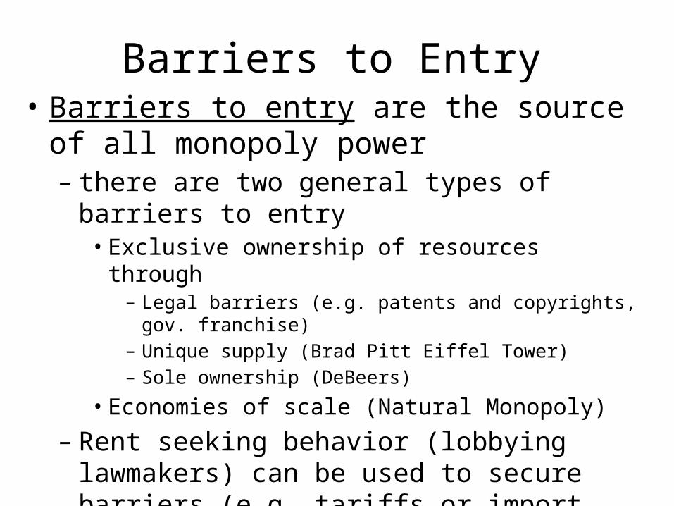
Barriers to Entry• Barriers to entry are the source of all monopoly
power– there are two general types of barriers to entry
• Exclusive ownership of resources through– Legal barriers (e.g. patents and copyrights, gov. franchise)– Unique supply (Brad Pitt Eiffel Tower)– Sole ownership (DeBeers)
• Economies of scale (Natural Monopoly)
– Rent seeking behavior (lobbying lawmakers) can be used to secure barriers (e.g. tariffs or import restrictions)

Price Setters
• Single Price Monopolist– Assume they cannot price discriminate, or behave
strategically.– Monopoly or Monopolistic Competition
• Price Discrimination– first, second and third degree
Revenue: Price Setter
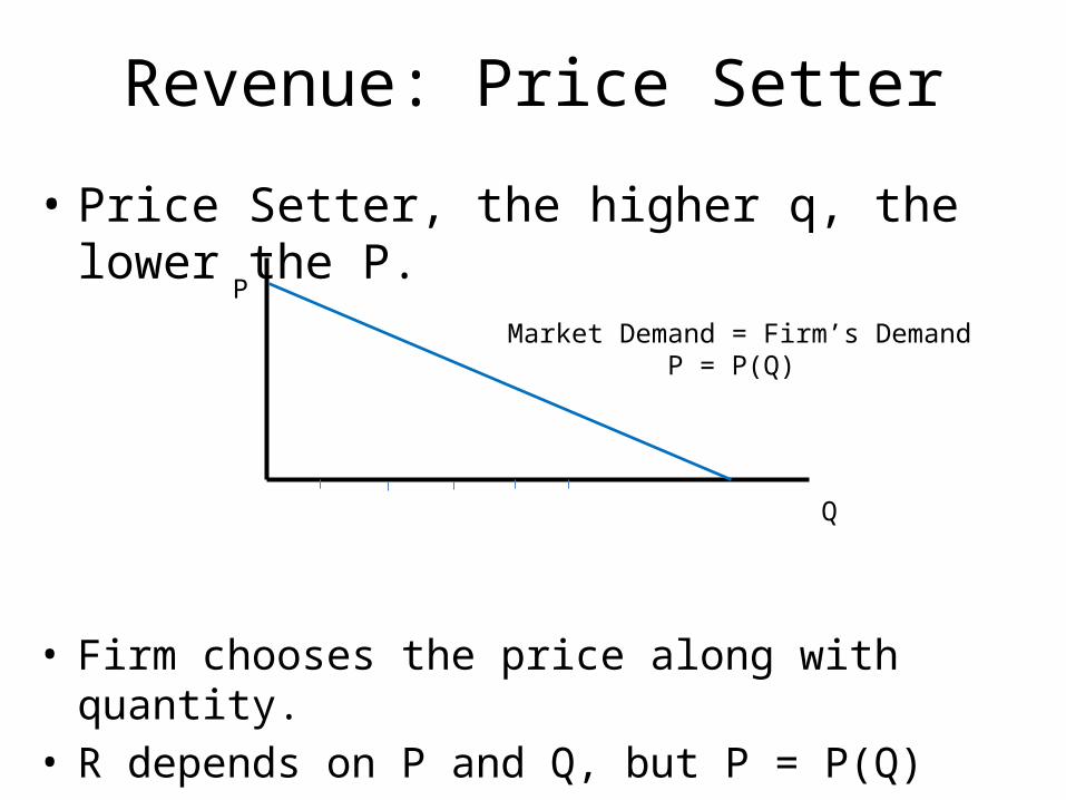
• Price Setter, the higher q, the lower the P.
• Firm chooses the price along with quantity.• R depends on P and Q, but P = P(Q)• R = P(Q)·Q
P
Q
Market Demand = Firm’s DemandP = P(Q)
Revenue: Price Setter
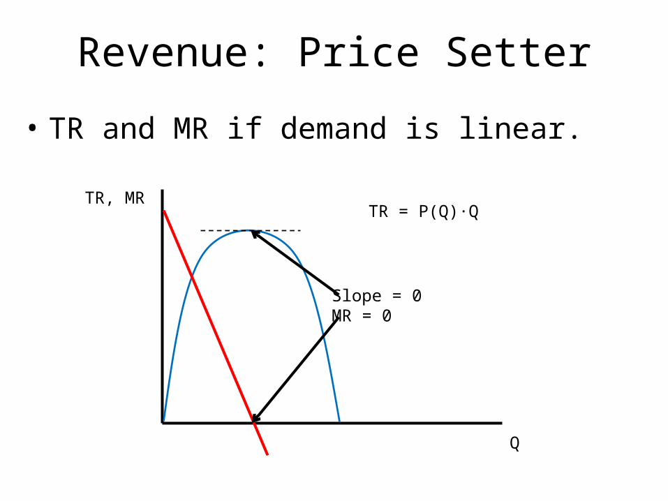
• TR and MR if demand is linear.
TR, MR
Q
Slope = 0MR = 0
TR = P(Q)·Q
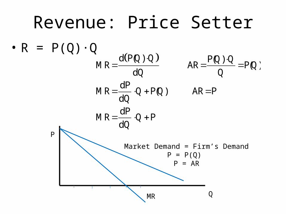
Revenue: Price Setter• R = P(Q)·Q
P
Q
Market Demand = Firm’s DemandP = P(Q) P = AR
MR
d P(Q) Q P(Q) QMR AR P(Q)
dQ QdP
MR Q P(Q) AR PdQdP
MR Q P dQ
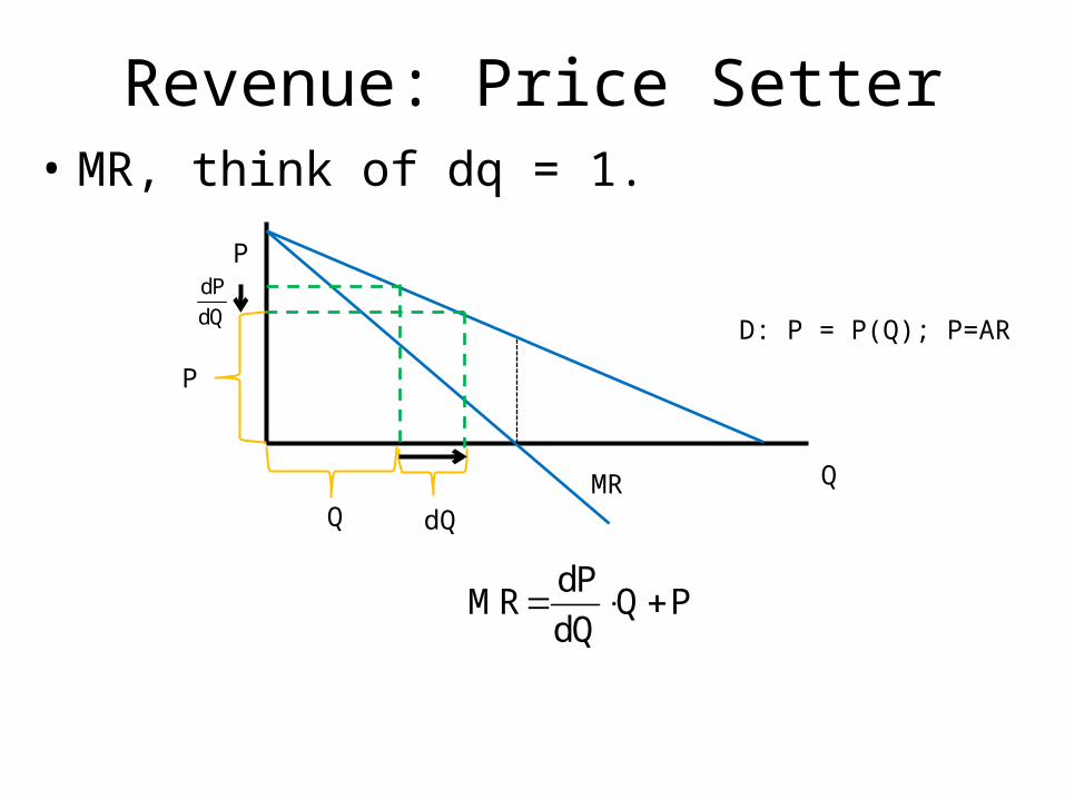
Revenue: Price Setter• MR, think of dq = 1.
P
Q
D: P = P(Q); P=AR
MR
dPMR Q P
dQ
dPdQ
Q dQ
P

Revenue: Price Setter• MR, think of dQ = 1.
• MR clearly depends on e.
P
Q
D: P = P(Q); P=AR
MRQ dQ
P
elastic
inelasticdPdQ
dPMR Q P
dQ
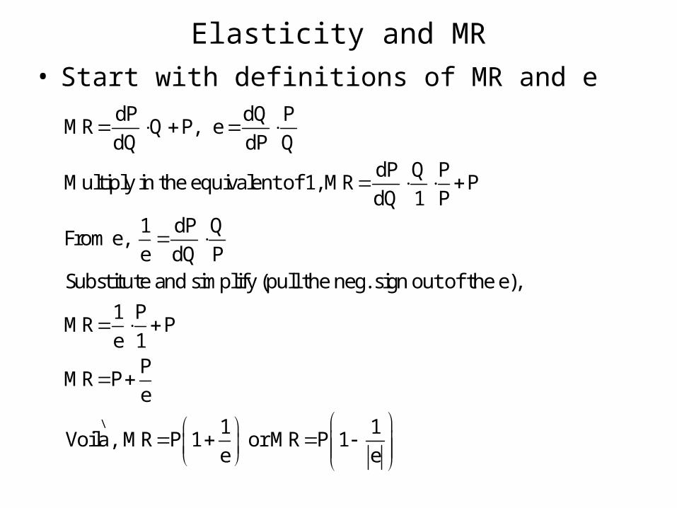
Elasticity and MR• Start with definitions of MR and e
\
dP dQ PMR Q P, e
dQ dP QdP Q P
Multiply in the equivalent of 1, MR PdQ 1 P
1 dP QFrom e,
e dQ PSubstitute and simplify (pull the neg. sign out of the e),
1 PMR P
e 1P
MR Pe
1Voila, MR P 1 or MR P 1
e
1e
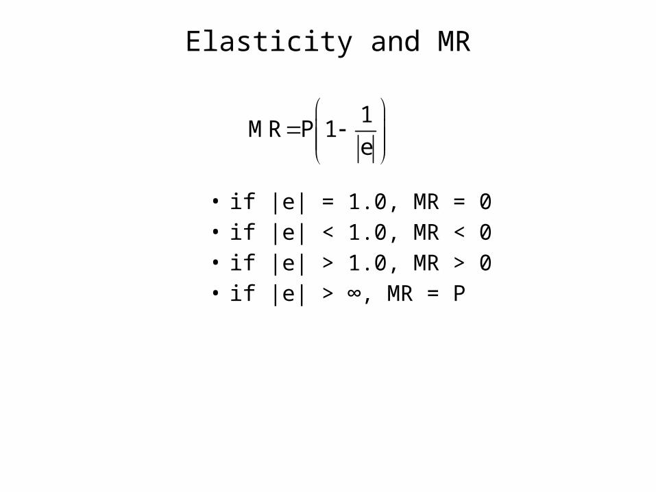
• if |e| = 1.0, MR = 0 • if |e| < 1.0, MR < 0• if |e| > 1.0, MR > 0• if |e| > ∞, MR = P
1MR P 1
e
Elasticity and MR
Firm Supply Decision
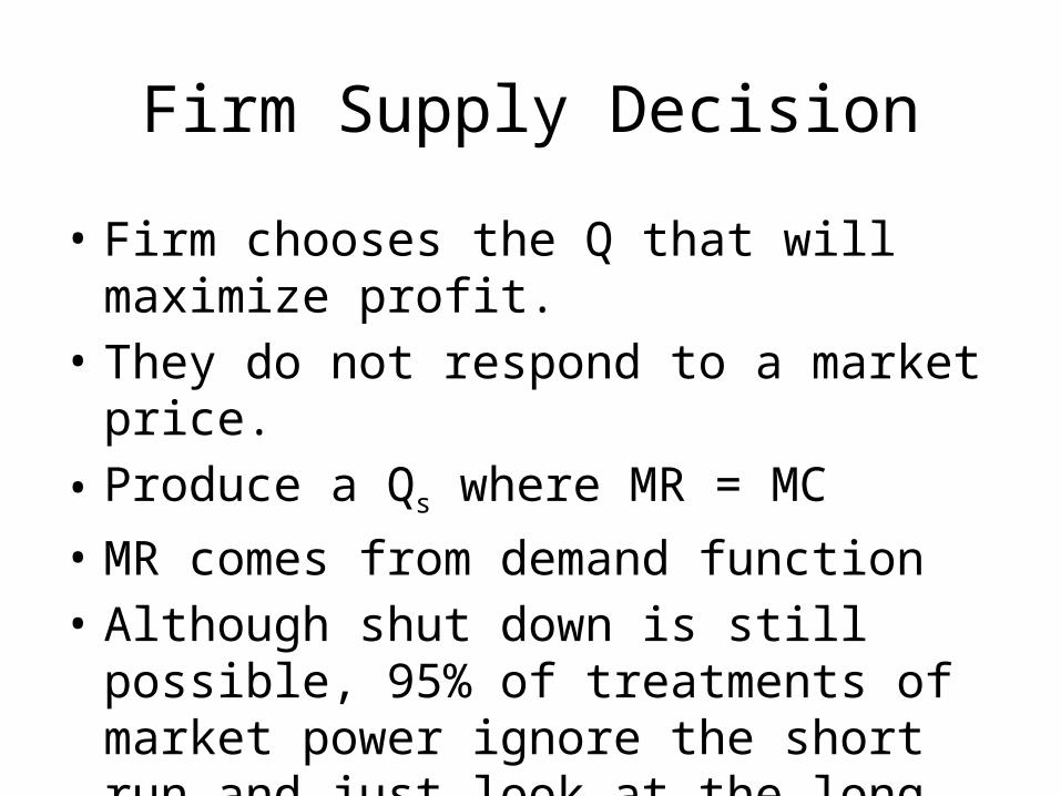
• Firm chooses the Q that will maximize profit. • They do not respond to a market price.• Produce a Qs where MR = MC• MR comes from demand function• Although shut down is still possible, 95% of
treatments of market power ignore the short run and just look at the long run.
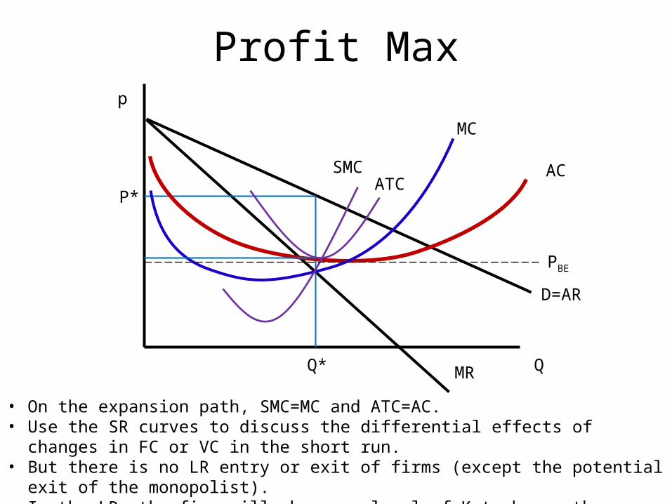
Profit Maxp
Q
D=AR
MC
MRQ*
P*
ACSMCATC
• On the expansion path, SMC=MC and ATC=AC. • Use the SR curves to discuss the differential effects of changes in FC or VC in the short run.• But there is no LR entry or exit of firms (except the potential exit of the monopolist).• In the LR, the firm will choose a level of K to be on the expansion path, so long as P > AC.
PBE
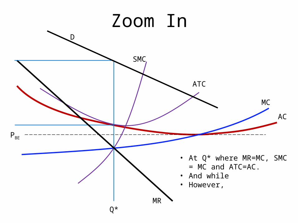
Zoom In
MC
AC
SMC
ATC
• At Q* where MR=MC, SMC = MC and ATC=AC.
• And while • However,
PBE
MRQ*
D
Price Setter in the Long Run
• Simple, just MR = MC• Maximize profit w.r.t. Q• Maximize profit w.r.t. K, L
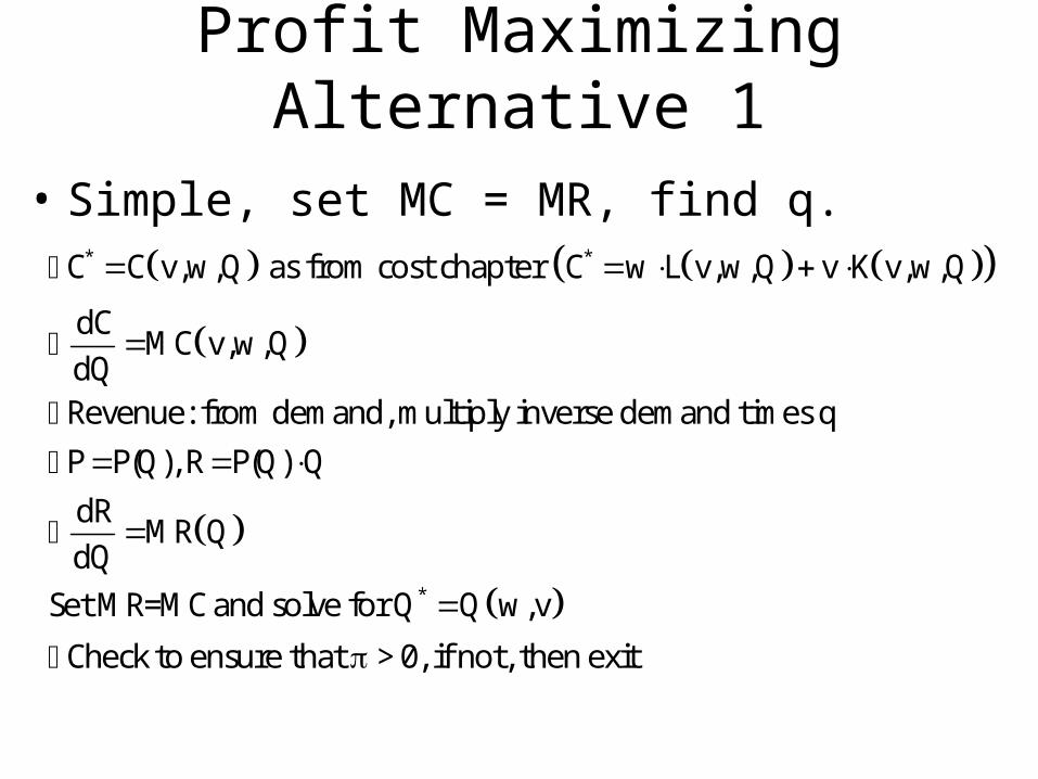
Profit Maximizing Alternative 1
• Simple, set MC = MR, find q.
* *
*
C C v,w,Q as from cost chapter C w L v,w,Q v K v,w,Q
dC MC v,w,QdQ
Revenue: from demand, multiply inverse demand times q P P(Q), R P(Q) Q
dR MR Q dQ
Set MR=MC and solve for Q Q w,v
Check to ensure
that > 0, if not, then exit
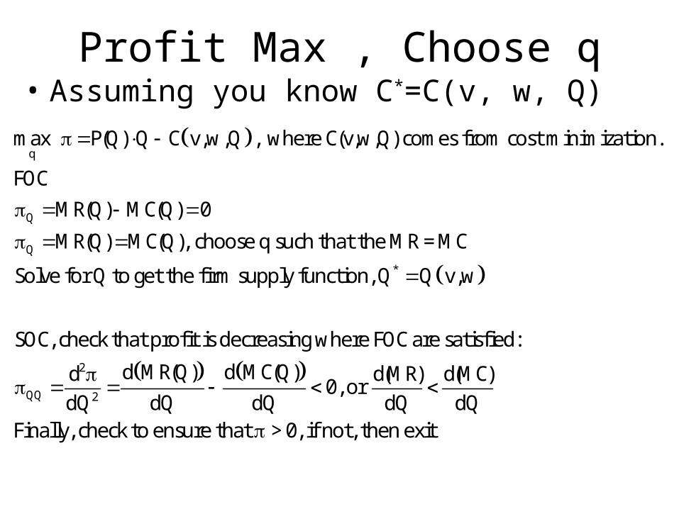
Profit Max , Choose q• Assuming you know C*=C(v, w, Q)
q
Q
Q
*
max P(Q) Q C v,w,Q , where C(v,w,Q) comes from cost minimization.
FOCMR(Q) MC(Q) 0
MR(Q) MC(Q), choose q such that the MR = MC
Solve for Q to get the firm supply function, Q Q v,w
SOC, check that
2
QQ 2
profit is decreasing where FOC are satisfied:
d MR(Q) d MC(Q)d d(MR) d(MC)0, or
dQ dQ dQ dQ dQFinally, check to ensure that > 0, if not, then exit
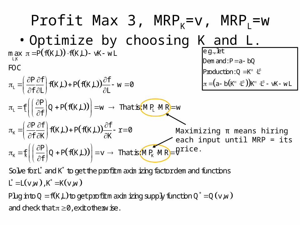
Profit Max 3, MRPK=v, MRPL=w• Optimize by choosing K and L.
L ,K
L
L L L
K
K K K
max P f K,L f K,L vK wL
FOC
P fff K,L P f K,L w 0
f L L
Pf Q P f K,L w That is: MP MR w
f
P fff K,L P f K,L r 0
f K K
Pf Q P f K,L v That is: MP MR v
f
S
* *
* *
*
olve for L and K to get the profit maximizing factor demand functions
L L v,w , K K v,w
Plug into Q f K,L to get profit maximizing supply function Q Q v,w
and check that 0, exit otherwise.
e.g., letDemand: P a bQ
Production: Q K L
a b K L K L vK wL
Maximizing π means hiring each input until MRP = its price.
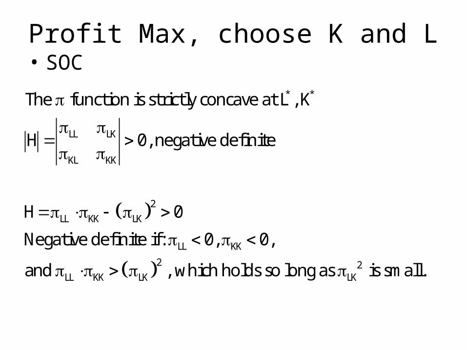
Profit Max, choose K and L• SOC
* *
LL LK
KL KK
2LL KK LK
LL KK
2 2LL KK LK LK
The function is strictly concave at L , K
H 0, negative definite
H 0
Negative definite if: 0, 0,
and , which holds so long as is small.

Profit Max, choose K and L
• Profit function, maximal profits for a given w, v.
* *Plug K =K(v,w) and L L(v,w) into
P f K,L f K,L vK wL
to get the profit optimizing profit function:
P f K(v,w),L(v,w) f K(v,w),L(v,w) vK(v,w) wL(v,w)
Note, there is no P in this equation as determining prof
it maximizing K and L determines Q*, which sets P* according to demand.
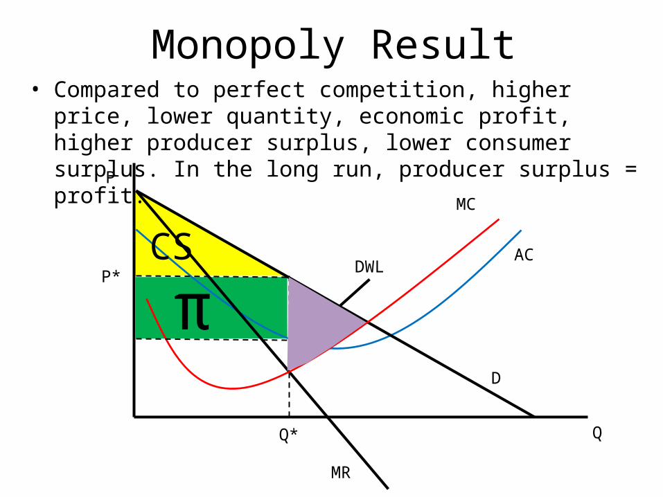
Monopoly Result• Compared to perfect competition, higher price, lower quantity,
economic profit, higher producer surplus, lower consumer surplus. In the long run, producer surplus = profit.
Q*
P
Q
MR
MC
AC
D
P*
πDWL
CS

Competitive Comparison• In long run, no profit or producer surplus (constant cost case
anyway).• Because of the deadweight loss from monopoly, it is considered a
market failure.P
Q
MR
Competitive Market supply = Market MC
AC
D
CS
QCQM
PM
PC

The Inverse Elasticity Rule
1MRis defined as MR P 1
e
When maximizing profit, MC MR, so the folowing must hold:
1 1MC P 1 or MC =P 1
e e
Since monopolists only produce where e -1 MC will always the price.For exa
mple
1e = -2, MC = P
23
e = -4, MC = P4
e = - , MC = P
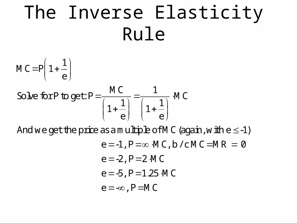
The Inverse Elasticity Rule
1MC P 1
eMC 1
Solve for P to get: P MC1 1
1 1e e
And we get the price as a multiple of MC (again, with e -1) e -1, P MC, b / c MC MR 0
e -2, P 2 MC e -5, P 1.25 MC e - , P MC
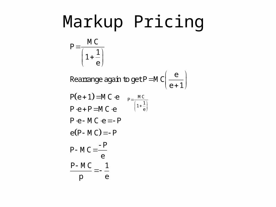
Markup Pricing
MCP
11
ee
Rearrange again to get P MCe 1
P e 1 MC e
P e P MC eP e MC e P
e P MC P
PP MC
eP MC 1
p e
MCP
11
e

The Inverse Elasticity Rule• The gap between a firm’s price and its marginal cost is
inversely related to the price elasticity of demand facing the firm
1P MCP e
P
QMR
MC
D, P = P(Q)P
p-MC
For -1 < e < 0,the markup exceeds the price. Huh?

The Inverse Elasticity Rule
• If e = -1, P-MC = P, the markup is p (since MC must = 0)• If e = -1.25, the markup is 80% of price• If e = -2, the markup with be 50% of price• If e = -5, the markup will be 20% of price• If e = -20, the markup will be 5% of price
P MC 1P e

Change in Price for a Change in MC
MCP
11
eP 1
, when e -1 1MC 1e
For exampleP
e=-2, 2, so price rises by twice the change in MC.MCP
e=-5, 1.25, so price rises by 1.25 x the change in MC.MC
Pe 10, 1.11, so price ris
MC
es by 1.11 x the change in MC.
MCP
11
e

Natural Monopoly• In a competitive market, so many firms can
produce at the Minimum Efficient Scale (MES) – low point of AC curve – that no firm can change the market price by altering its behavior.
• But if the MES is large enough that it only takes a few firms to supply the market, they will start to have market power.
• If MES is so large that one firm can produce at a lower average cost than two firms can splitting the market in half, then we get a natural monopoly.
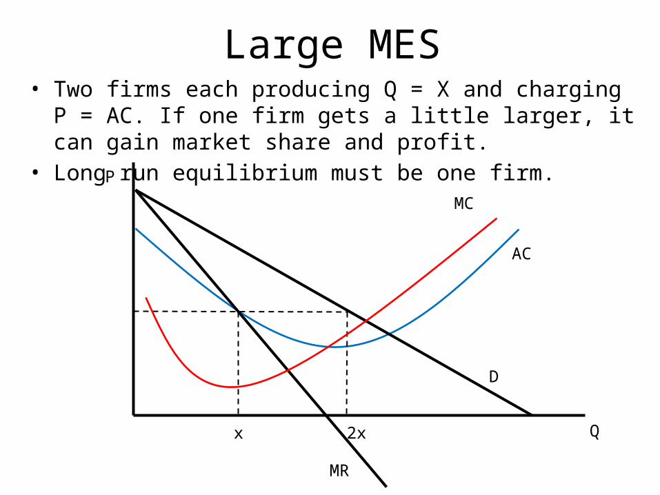
Large MES• Two firms each producing Q = X and charging P = AC. If one firm
gets a little larger, it can gain market share and profit.• Long run equilibrium must be one firm.
x 2x
P
Q
MR
MC
AC
D
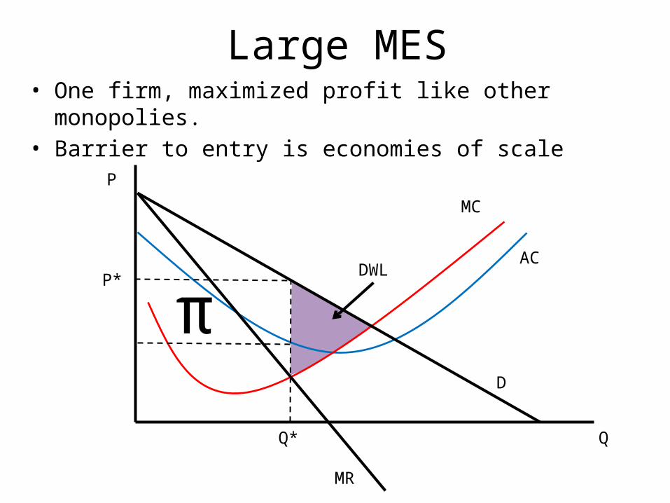
Large MES• One firm, maximized profit like other monopolies.• Barrier to entry is economies of scale
Q*
P
Q
MR
MC
AC
D
P*
πDWL

Regulating This Monopoly• Considered regular monopoly.• Regulate price where MC = demand• Profit > 0.
QR
P
Q
MR
MC
AC
D
PR π
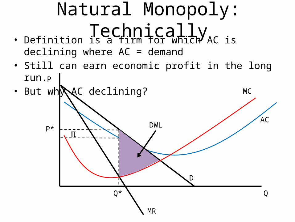
Natural Monopoly: Technically• Definition is a firm for which AC is declining where AC = demand• Still can earn economic profit in the long run.• But why AC declining?
P
Q
MR
MC
AC
D
Q*
P* πDWL

Natural Monopoly: Technically• If AC declining at intersection with demand, it requires MC < AC
where MC=MB.• Sadly, regulation cannot require MC=MB without firm exit.
P
Q
MR
MC
AC
D
QR
PRLoss
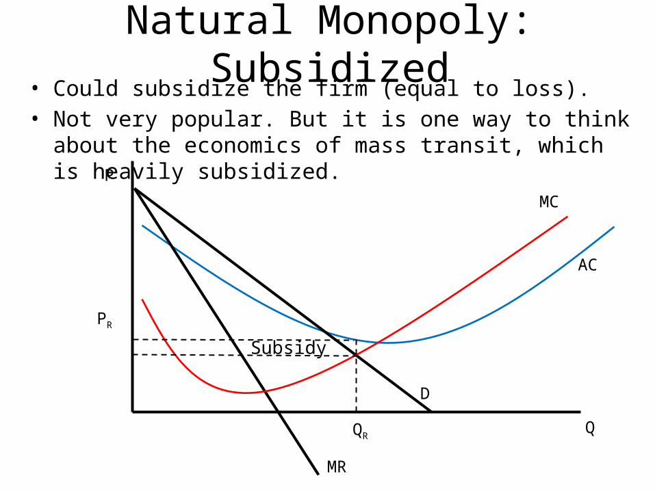
Natural Monopoly: Subsidized• Could subsidize the firm (equal to loss).• Not very popular. But it is one way to think about the economics
of mass transit, which is heavily subsidized.P
Q
MR
MC
AC
D
QR
PR
Subsidy

Natural MonopolyAverage Cost Pricing
• Average cost pricing regulation ensures continued production.• DWL results, but it is the more usual strategy.
P
Q
MR
MC
AC
D
QR,ACP
PR,ACP
DWL
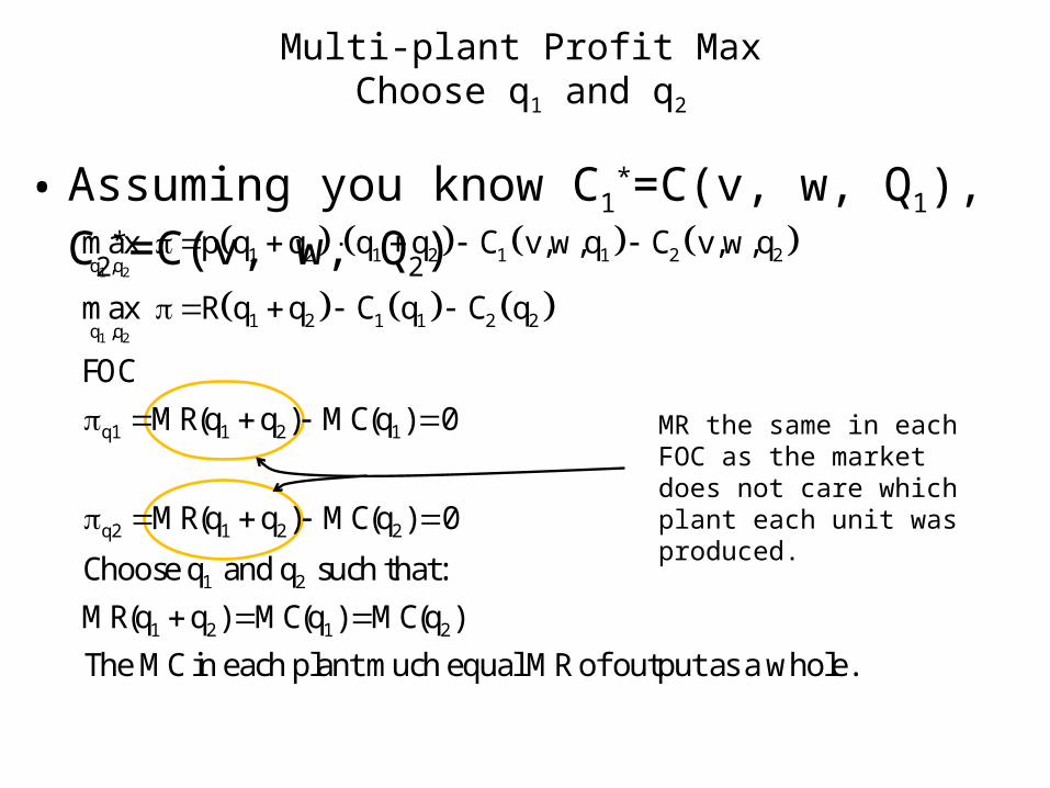
Multi-plant Profit MaxChoose q1 and q2
• Assuming you know C1*=C(v, w, Q1), C2
*=C(v, w, Q2)
1 2
1 2
1 2 1 2 1 1 2 2q ,q
1 2 1 1 2 2q ,q
q1 1 2 1
q2 1 2 2
1 2
1 2 1 2
max p q q q q C v,w,q C v,w,q
max R q q C q C q
FOCMR(q q ) MC(q ) 0
MR(q q ) MC(q ) 0
Choose q and q such that:MR(q q ) MC(q ) MC(q ) The MC in each plant much equal
MR of output as a whole.
MR the same in each FOC as the market does not care which plant each unit was produced.

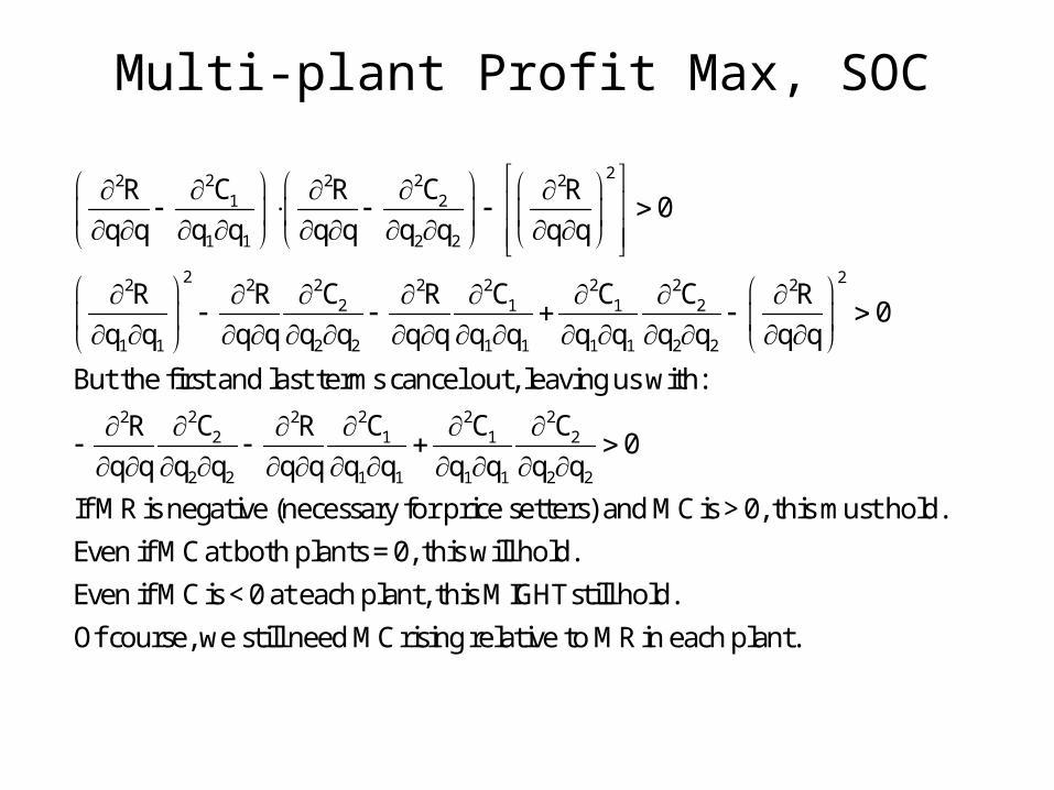
Multi-plant Profit Max, SOC
2 2 2
1 1 1 1 1 2
21
1 1
SOC, profit decreasing (MR falling faster than MC -- easy if MR falling and MC rising)
R R Rslope of total MR curve = ,
q q q q q q
Cslope of each plant's MC curves: plant 1: , p
q q
21
1 1
221
1 1 1 1
222
2 2 2 2
22 21
1 1 1 1 1 2
2
Clant 2:
q q
CR0, MC in plant 1 must be rising relative to MR
q q q q
CR0, MC in plant 2 must be rising relative to MR
q q q qNow the Hessian:
CR Rq q q q q q
22 22 2 21 2
221 1 1 1 2 2 2 2 1 22
2 1 2 2 2 2
C CR R R0
q q q q q q q q q qCR Rq q q q q q
Let's break this down on the next slide...
Multi-plant Profit Max, SOC22 22 2 2
1 2
1 1 2 2
2 22 2 2 22 2 2 22 1 1 2
1 1 2 2 1 1 1 1 2 2
C CR R R0
q q q q q q q q q q
C C C CR R R R0
q q q q q q q q q q q q q q q q
But the first and last terms cancel
2 2 2 22 22 1 1 2
2 2 1 1 1 1 2 2
out, leaving us with:
C C C CR R0
q q q q q q q q q q q qIf MR is negative (necessary for price setters) and MC is > 0, this must hold.Even if MC at both plants = 0, this will h
old.Even if MC is < 0 at each plant, this MIGHT still hold.Of course, we still need MC rising relative to MR in each plant.

Graphically
$
q1 q2
MC2MC1 MCT MCT
MR
D
p
q1+q2=Q
Example
1 22 2
1 1 2 22 2
1 2 1 2
1 2 11
1 2 22
1
2 2
2
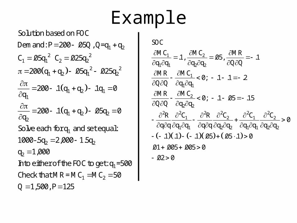
Solution based on FOCDemand: P 200 .05Q, Q=q q
C .05q C .025q
200 q q .05q .025q
200 .1 q q .1q 0q
200 .1 q q .05q 0q
Solve each for q and set equal:1000-.5q 2,000 1.5qq 1
1
1 2
,000Into either of the FOC to get: q =500Check that MR = MC MC 50Q 1,500, P 125
1 2
1 1 2 2
1
1 1
2
2 22 2 2 22 2
1 2 1 2
1 1 2 2 1 1 2 2
SOCMC MC MR
.1, .05, .1q q q q Q Q
MCMR0; .1 .1 .2
Q Q q qMCMR
0; .1 .05 .15Q Q q q
C C C CR R0
q q q q q q q q q q q q
.1 .1 .1 .05 .05 .1 0
.01 .0
05 .005 0.02 0
Monopoly and Quality
• Firms purposely make goods less durable than they could so that we have to buy replacements more often!

Monopoly and Quality• Demand
• Profit
P P(Q,X), Q is quantity and X is qualityP P
0, 0Q X
P(Q,X) Q C(Q,X)FOC
P C P CP(Q,X) Q 0 Q P
Q Q Q Q Q
P C P CQ 0 Q
X X X X X
MR MC
MRx MCx
So long as Q* such that MR = MC, also set the MR from an increase in X = the MC of that extra X.
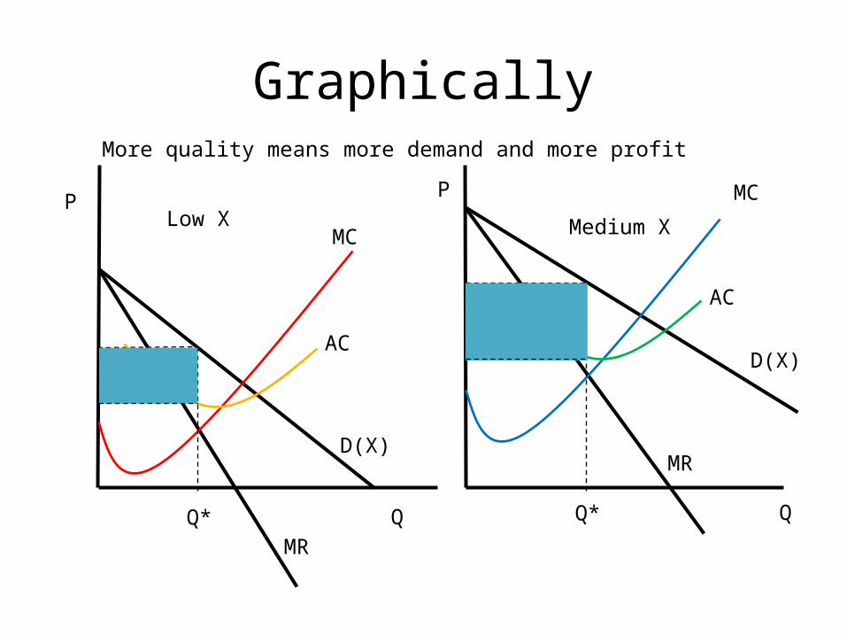
Graphically
MR
D(X)
P
QQ*
P
More quality means more demand and more profit
MR
D(X)
QQ*
MC
MC
AC
AC
Low X Medium X

Graphically
MR
D(X)
P
QQ*
But only to a point
MR
D(X)
P
QQ*
MC
AC
MC
AC
Medium XHigh X

Monopoly and Tax Policy
• Flat Tax (tax = t)• Unit Tax (tax = tQ)• Revenue Tax (tax = t·R(Q))• Profit (Earnings) Tax (tax = t·π)• For each, start with revenue function and total
cost function (C*).• R=R(Q) =P(Q)*Q• C*=C(Q)
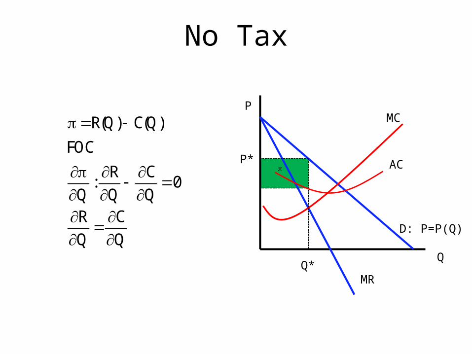
No Tax
R(Q) C(Q)FOC
R C: 0
Q Q QR CQ Q
P
Q
MC
D: P=P(Q)
MR
Q*
P* AC

t
Flat Tax( t > 1)
R(Q) C(Q) tFOC
R C: 0
Q Q QR CQ Q
Same result as no tax.
P
Q
MC
D: P=P(Q)
MR
AC
ACt
Q*t
P*t

Unit Tax( t > 0)
*t
R(Q) C(Q) tQ
FOCR C
: t 0Q Q QR C
tQ Q
Different output from no tax. R C
Q where Q Q
P
Q
MC
D: P=P(Q)
MR
t
Q*t
P*t
AC
ACt=AC+t
MCt=MC+t

Revenue Tax(0 < t < 1)
*t
R(Q) 1 t C(Q)
FOCR C
: 1 t 0Q Q QR C
1 tQ Q
Different result from no tax. R C
Q where Q Q
P
Q
MC
D
P(1-t)
MRMRt=MR(1-t)
t
AC
Q*t
P*t
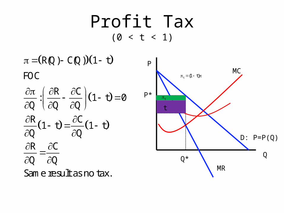
Profit Tax(0 < t < 1)
R(Q) C(Q) 1 t
FOC
R C: 1 t 0
Q Q QR C
1 t 1 tQ QR CQ Q
Same result as no tax.
P
Q
MC
D: P=P(Q)
MR
t (1 t)
tt
Q*
P*
Monopolistic Competition in Long Run
• In the short run if π > 0, then there is no difference between a monopoly and a monopolistically competitive firm.
• But despite the fact that firms have market power, there are firms providing close enough substitutes that demand for all firms falls to a level where π = 0.
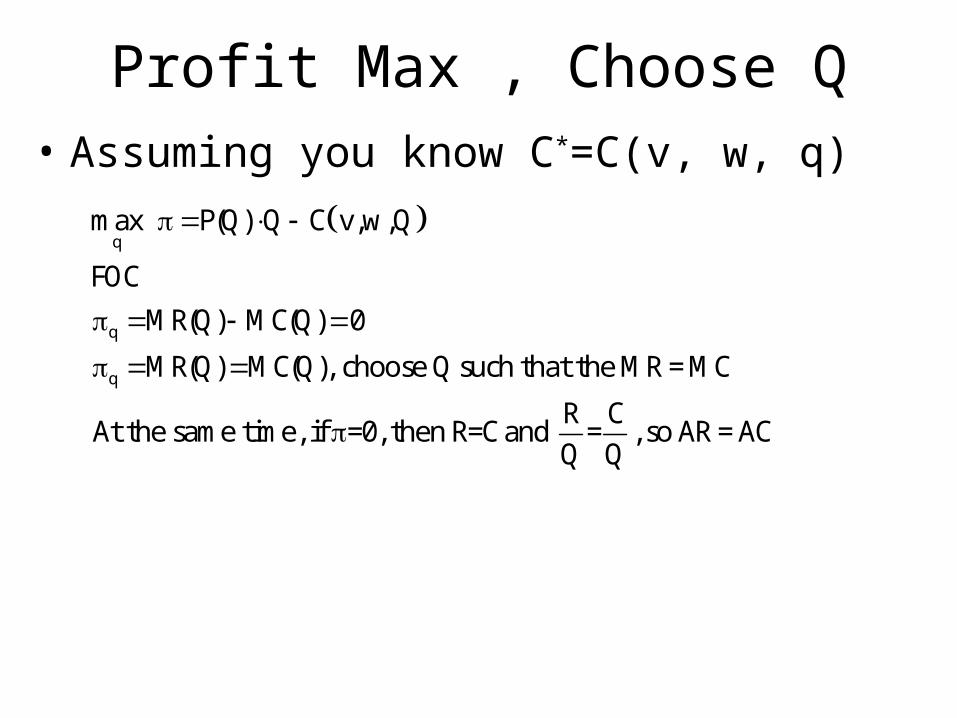
Profit Max , Choose Q• Assuming you know C*=C(v, w, q)
q
q
q
max P(Q) Q C v,w,Q
FOCMR(Q) MC(Q) 0
MR(Q) MC(Q), choose Q such that the MR = MC
R CAt the same time, if =0, then R=C and = , so AR = AC
Q Q
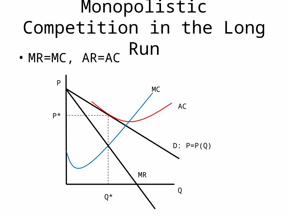
Monopolistic Competition in the Long Run
• MR=MC, AR=AC
MR
D: P=P(Q)
P
QQ*
MC
ACP*
Price Discrimination
• 1st degree• 2nd degree• 3rd degree
• Note, “1”, “2”, “3” mean nothing.

First Degree, Perfect Price Discrimination
• All buyers are charged a price equal to their willingness to pay. TC in green, TR = blue+green.
• No DWL• No CS either
– Car dealerships– Colleges– Reverse Auction
• Priceline
P=MR
D: P=P(Q)
P
qq*
MC
AC
Third Degree Price Discrimination
• Firm can separate demanders with different demand elasticities and charge different prices to each group.
• A single price must be charged to all consumers in each demand group.
• Arbitrage must be prevented.
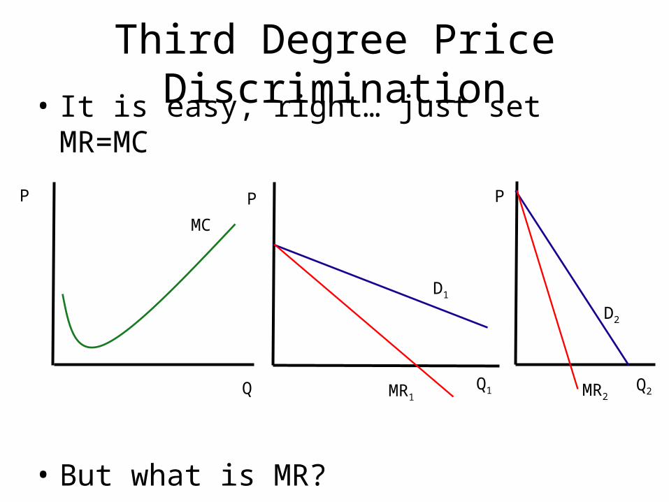
Third Degree Price Discrimination• It is easy, right… just set MR=MC
• But what is MR?
P P
Q
MC
D2
MR2MR1
P
Q1
D1
Q2
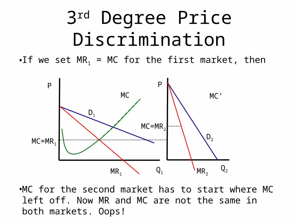
• If we set MR1 = MC for the first market, then
• MC for the second market has to start where MC left off. Now MR and MC are not the same in both markets. Oops!
P P
Q1Q2
MC
D2
MR2MR1
D1
MC=MR1
MC=MR2
3rd Degree Price Discrimination
MC’
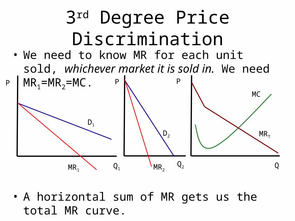
• We need to know MR for each unit sold, whichever market it is sold in. We need MR1=MR2=MC.
• A horizontal sum of MR gets us the total MR curve.• Set MC = MRT to get the P that allows MR1=MR2=MC
P P
Q1Q2
MC
D2
MR2MR1
P
Q
D1
MRT
3rd Degree Price Discrimination

• Set that MC =MR1=MR2 to get the q in each market.
• At those q, use demand to get the P in each market to maximize profit. MR1=MR2, but P1≠P2
PMC
D2
MR2MR1
D1
MRT
3rd Degree Price Discrimination
P
Q
P
Q2Q1

The Math• Max π = P1(Q1)•Q1+P2(Q2)•Q2-C(Q1+Q2)• FOC
• Solve for Q1 and Q2, then use demand curves to get P1 and P2
1 1 1
2 2 2
Q Q 1 Q 1 2
Q Q 2 Q 1 2
R (Q ) C (Q Q ) 0
R (Q ) C (Q Q ) 0

MR and Elasticity• Remember that with price setters:
• Since MR is the same for both markets
• And…
… so all you need is e1 and e2
1MR P 1
e
1 21 2
21
2
1
1 1MR P 1 P 1
e e
11
ePP 1
1e
Example
1
2
21 1 1 1 1
22 2 2 2 2
1 2
2 21 1 2 2 1 2
Q 1
Q 2
1 1 1
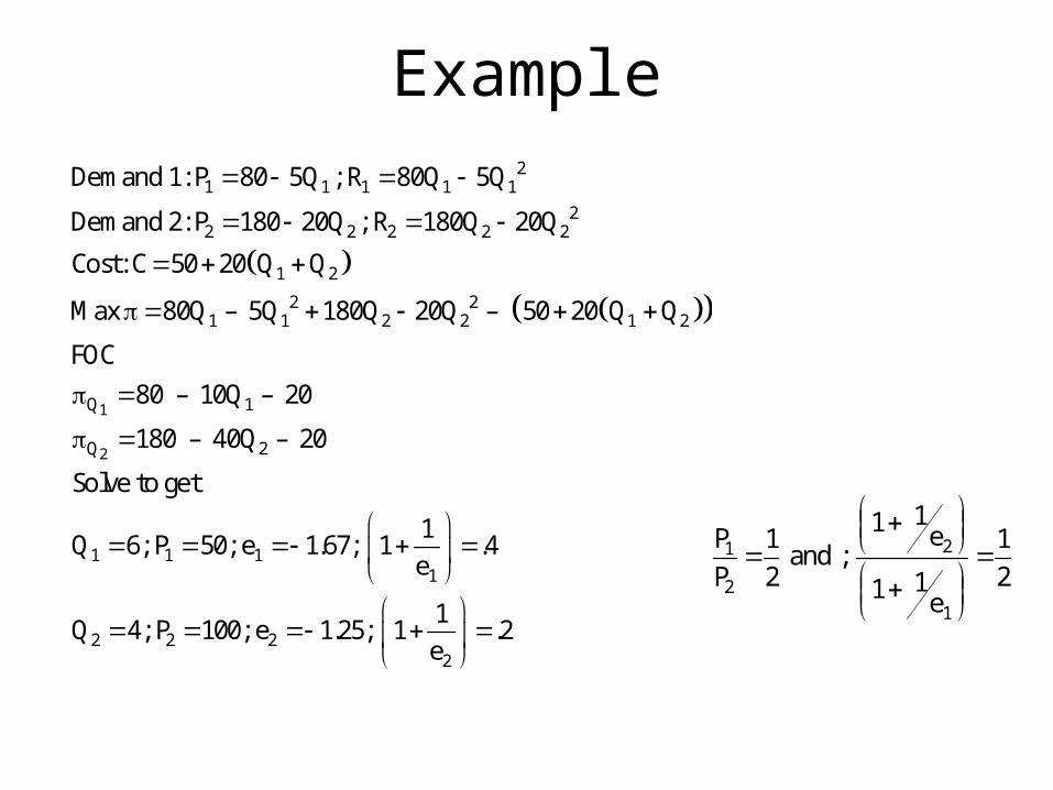
Demand 1: P 80 5Q ; R 80Q 5Q
Demand 2: P 180 20Q ; R 180Q 20Q
Cost: C 50 20 Q Q
Max 80Q – 5Q 180Q 20Q – 50 20 Q Q
FOC80 – 10Q – 20
180 – 40Q – 20
Solve to get
Q 6; P 50; e 1.67;
1
2 2 22
1 1 .4
e
1Q 4; P 100; e 1.25; 1 .2
e
21
21
11 eP 1 1 and ;
P 2 211 e

• Set that MC =MR1=MR2 to get the q in each market.
• At those q, use demand to get the P in each market to maximize profit. MR1=MR2, but P1≠P2
P P
Q Q
MC
D2
MR2MR1
P
Q
D1
MRT
3rd Degree Price Discrimination
6
50
4
100
20
6
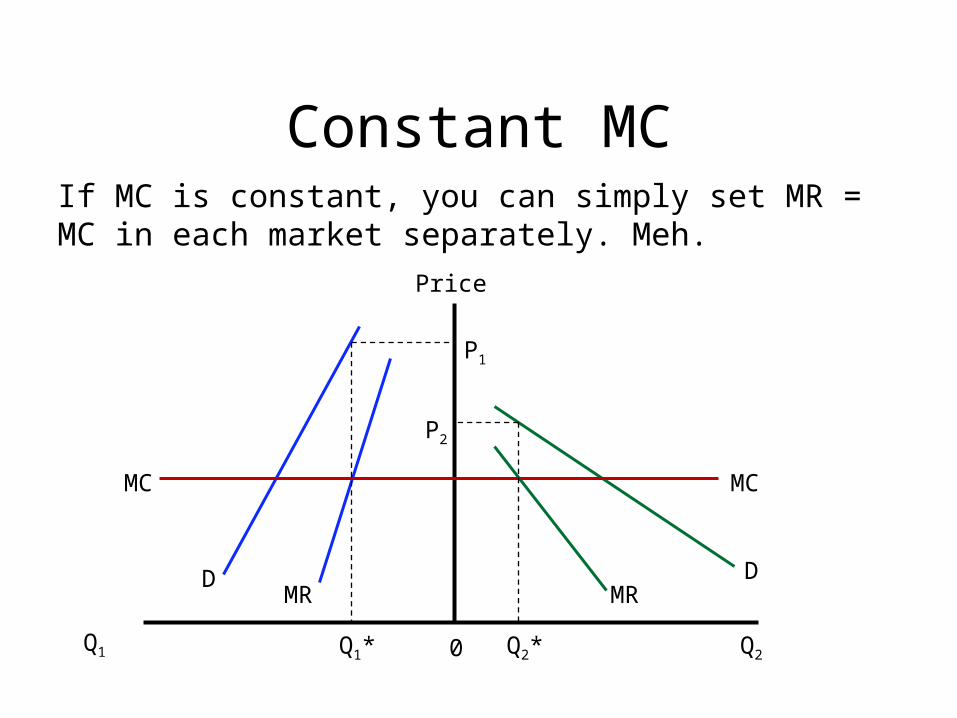
Constant MC
Q2Q1
Price
0
DDMRMR
MCMC
Q2*
P2
Q1*
P1
If MC is constant, you can simply set MR = MC in each market separately. Meh.
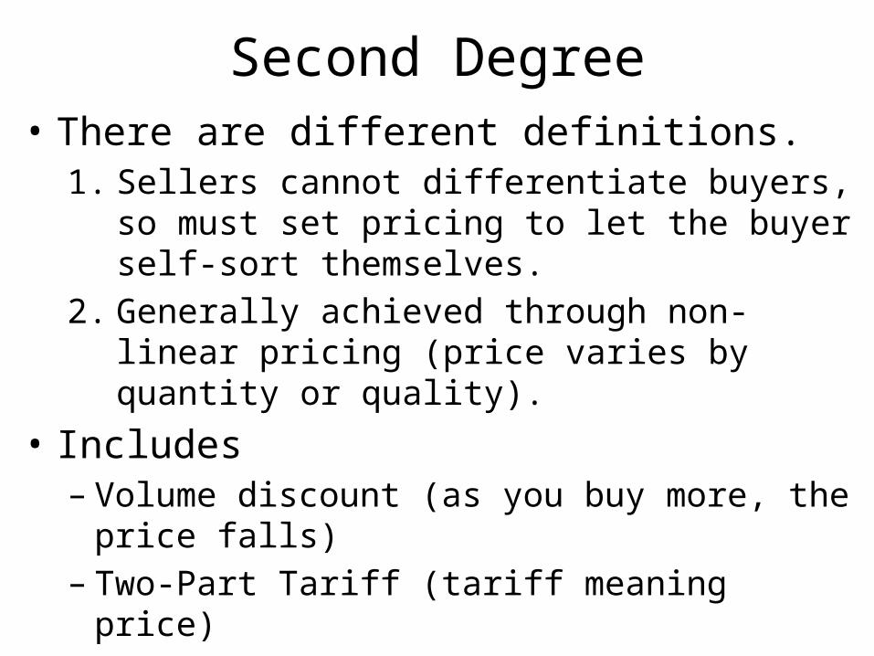
Second Degree• There are different definitions.
1. Sellers cannot differentiate buyers, so must set pricing to let the buyer self-sort themselves.
2. Generally achieved through non-linear pricing (price varies by quantity or quality).
• Includes– Volume discount (as you buy more, the price falls)– Two-Part Tariff (tariff meaning price)– Bundling

Volume Discount, Electricity• Graph is consumer specific• Consumer surplus now A + B + C• No so much a volume discount as a first use surcharge!
P
QQ3
MC=AC
A
B
PS C
P1
P2
P3
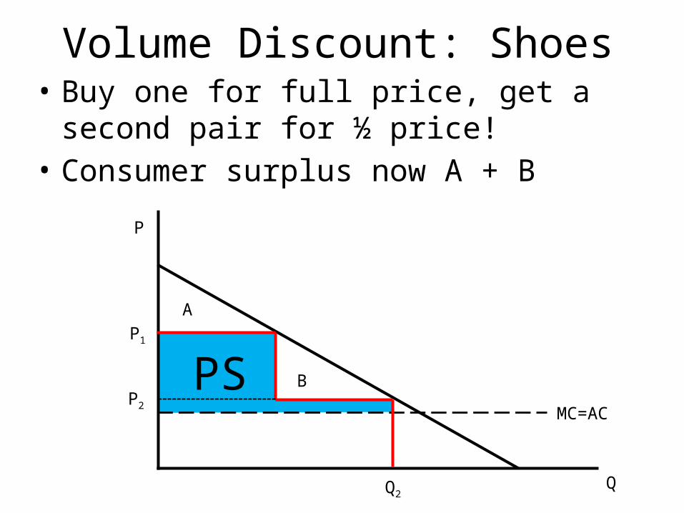
Volume Discount: Shoes• Buy one for full price, get a second pair for ½
price!• Consumer surplus now A + B
P
QQ2
MC=AC
A
BPSP1
P2
Two-Part Tariff• Tariff means “price”• First part is an “entry fee” and the second is
the per unit fee.• Even with volume discounts, we can think of
part of the initial higher price as an entry fee.• Some times the analysis is for the market and
sometimes consumer specific.
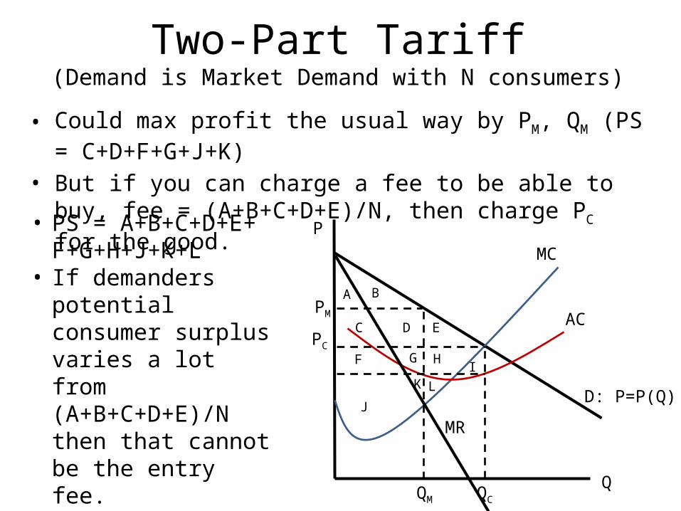
Two-Part Tariff(Demand is Market Demand with N consumers)
• Could max profit the usual way by PM, QM (PS = C+D+F+G+J+K)• But if you can charge a fee to be able to buy, fee =
(A+B+C+D+E)/N, then charge PC for the good.
MR
D: P=P(Q)
PMC
AC
Q
PM
PC
A B
C D E
F G H
QM QC
I
J
K L
• PS = A+B+C+D+E+ F+G+H+J+K+L
• If demanders potential consumer surplus varies a lot from (A+B+C+D+E)/N then that cannot be the entry fee.

Laser Printers• HP charges a low price for printers (the access fee)• However, if 10 buyers each have consumer surplus of $892 (from printer plus
ink) and the other 90 have CS = $12 each, entry fee is problematic.• When consumer demand varies a lot, low entry fee and higher unit price. For
printers, high demanders buy more as they use them up faster.
MR
D: P=P(Q)
PMC
AC
Q
PM
PC
A B
C D E
F G H
QM QC
I
J
K L
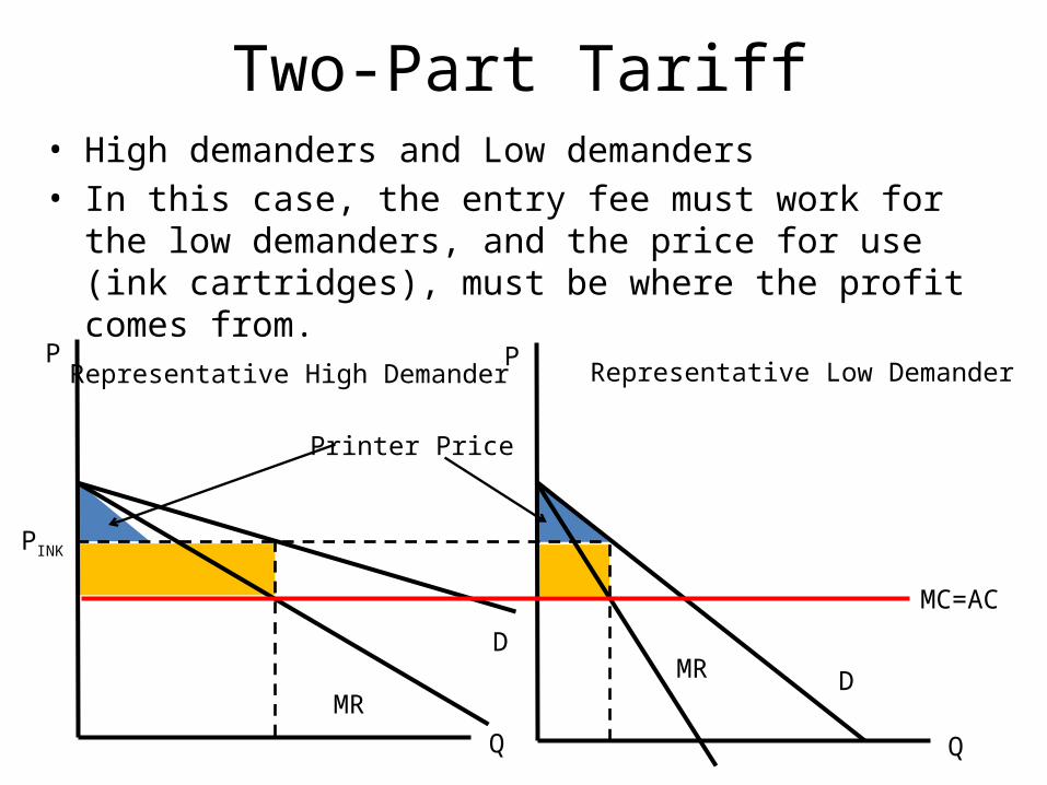
• High demanders and Low demanders• In this case, the entry fee must work for the low demanders,
and the price for use (ink cartridges), must be where the profit comes from.
Two-Part Tariff
MR
D
P
Q
PINK
MR D
P
MC=AC
Q
Printer Price
Representative Low DemanderRepresentative High Demander
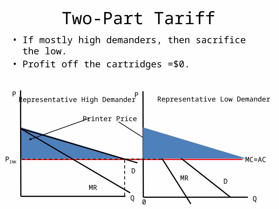
• If mostly high demanders, then sacrifice the low.• Profit off the cartridges =$0.
Two-Part Tariff
MR
D
P
Q
PINK
MR D
P
MC=AC
Q
Printer Price
Representative Low DemanderRepresentative High Demander
0
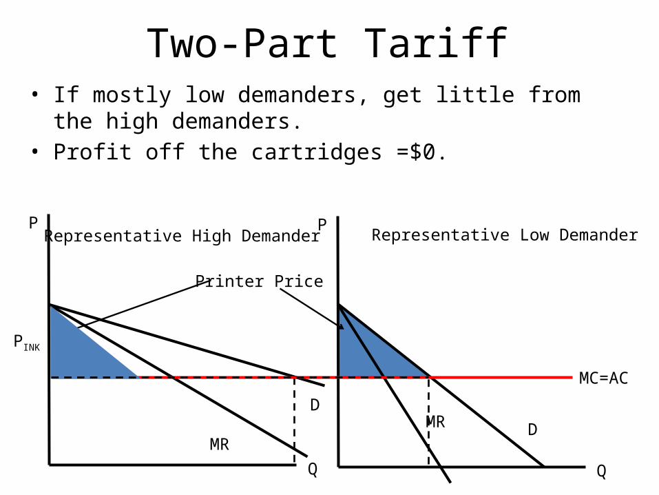
• If mostly low demanders, get little from the high demanders.• Profit off the cartridges =$0.
Two-Part Tariff
MR
D
P
Q
PINK
MR D
P
MC=AC
Q
Printer Price
Representative Low DemanderRepresentative High Demander
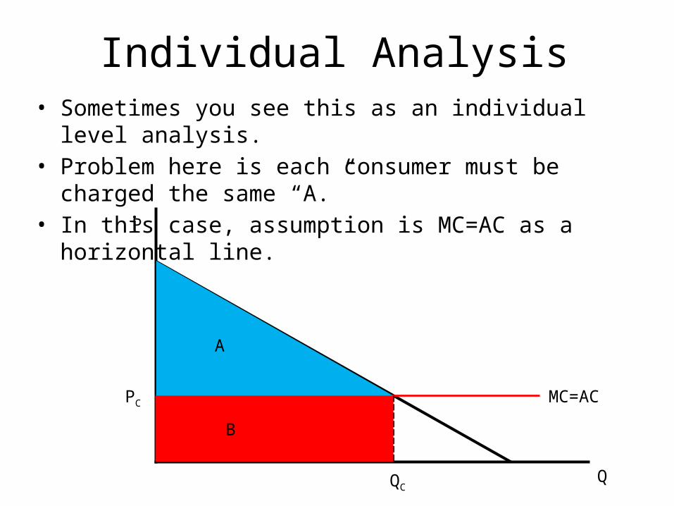
Individual Analysis• Sometimes you see this as an individual level analysis.• Problem here is each consumer must be charged the same “A.”• In this case, assumption is MC=AC as a horizontal line.
P
QQC
MC=AC
A
PC
B
Consumer Analysis: Golf Club
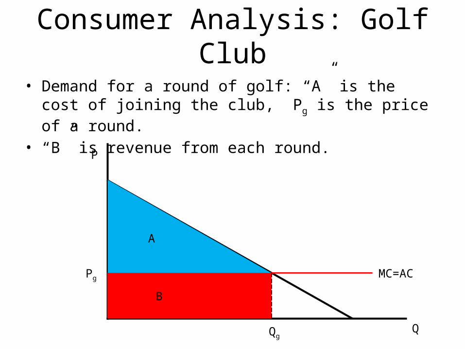
• Demand for a round of golf: “A” is the cost of joining the club, Pg is the price of a round.
• “B” is revenue from each round.
P
QQg
MC=AC
A
Pg
B
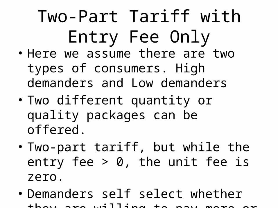
Two-Part Tariff with Entry Fee Only• Here we assume there are two types of
consumers. High demanders and Low demanders
• Two different quantity or quality packages can be offered.
• Two-part tariff, but while the entry fee > 0, the unit fee is zero.
• Demanders self select whether they are willing to pay more or less.
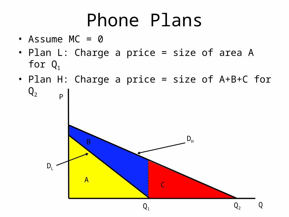
• Assume MC = 0• Plan L: Charge a price = size of area A for Q1
• Plan H: Charge a price = size of A+B+C for Q2
Phone Plans
DH
P
QQ1
DL
Q2
A
B
C
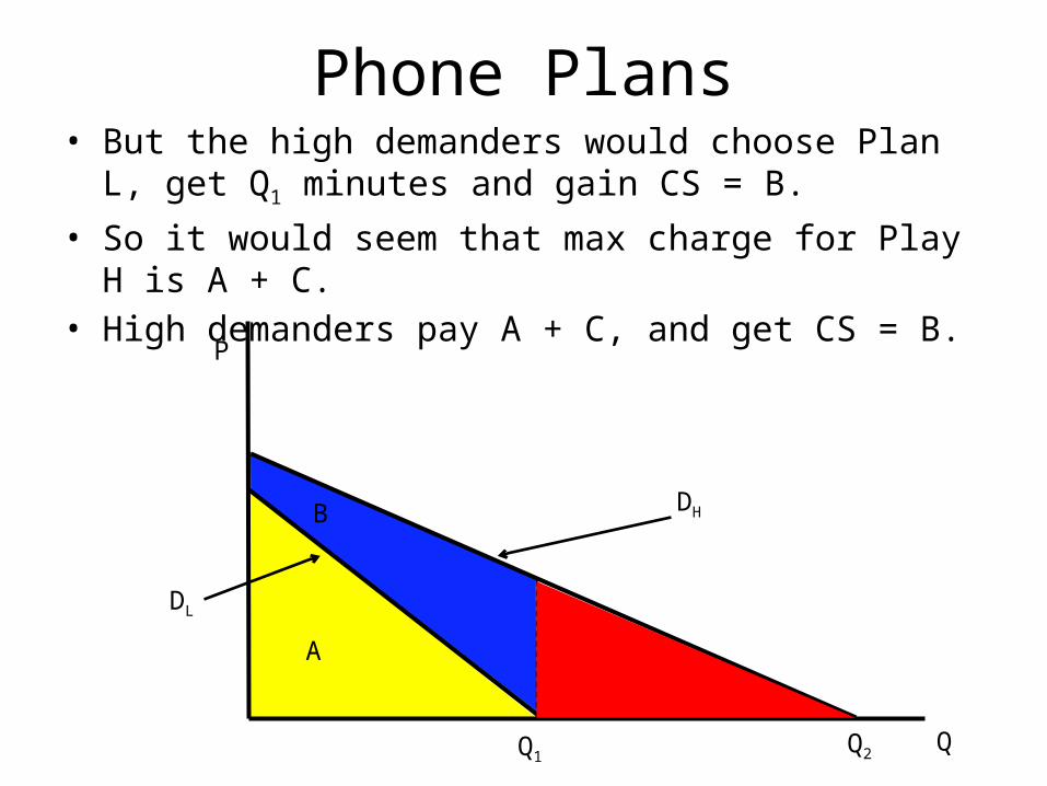
• But the high demanders would choose Plan L, get Q1 minutes and gain CS = B.
• So it would seem that max charge for Play H is A + C.• High demanders pay A + C, and get CS = B.
Phone Plans
DH
P
QQ1
DL
Q2
CA
B

• Even better, don’t offer Q1 as an option.
• Plan L: Q’1 minutes for a price of A.
• Plan H: Q2 minutes for a price of A + A’ + C + C’.• High demanders still choose Plan H, get CS = B (which is now
smaller)
Phone Plans
DH
P
QQ1
DL
Q2
C
• Profit gains C’ and loses A’
Q’1
A’
C’
A
B
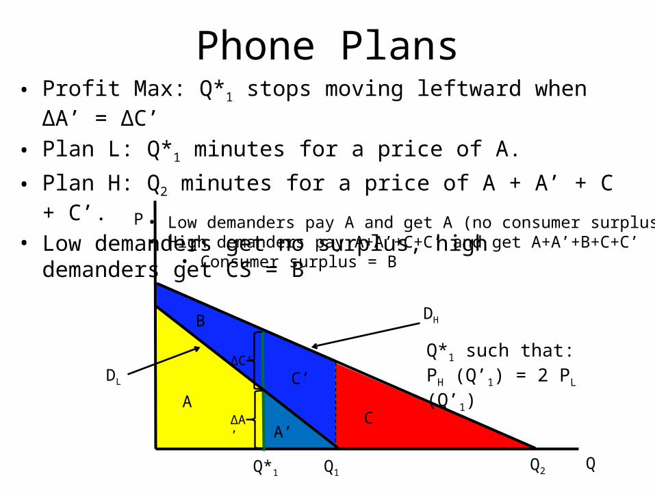
• Profit Max: Q*1 stops moving leftward when ΔA’ = ΔC’
• Plan L: Q*1 minutes for a price of A.
• Plan H: Q2 minutes for a price of A + A’ + C + C’.• Low demanders get no surplus, high demanders get CS = B
Phone Plans
DH
P
QQ1
DL
Q2
C
Q*1
ΔA’
C’A
B
ΔC’
A’
Q*1 such that: PH (Q’1) = 2 PL (Q’1)
• Low demanders pay A and get A (no consumer surplus)• High demanders pay A+A’+C+C’ and get A+A’+B+C+C’
• Consumer surplus = B
Quantity and Quality• Phone carriers offer plans with more or fewer
numbers of unlimited minutes.• But firms can vary quality instead of quantity.
– Airlines offer business and coach class.• Don’t alter quantity, but quality• Lower the coach quality to encourage high demanding
business travelers to pony up for business class.

Bundling• There are several items that different consumers
are willing to pay different amounts for, but we don’t know which items each consumers values most.
• This is a version of buy one pair, get a second for ½ price, but you cannot buy one pair.
Bundling
P
QQ=2
MC=AC
A
B
80
40
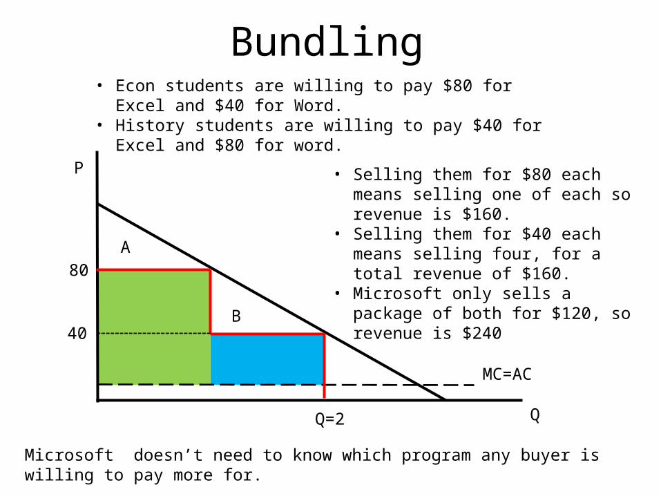
• Econ students are willing to pay $80 for Excel and $40 for Word.• History students are willing to pay $40 for Excel and $80 for word.
• Selling them for $80 each means selling one of each so revenue is $160.
• Selling them for $40 each means selling four, for a total revenue of $160.
• Microsoft only sells a package of both for $120, so revenue is $240
Microsoft doesn’t need to know which program any buyer is willing to pay more for.
Monopoly and Patents• New ideas (inventions, creative works, etc.) are costly to
produce.• Once created, intellectual property has a low cost of
distribution.• Perfect competition in production is assured.• No incentive to do the hard work of creation.• Writers of the US Constitution saw this
– Framers specified patent and copyright protection• Yet guaranteed monopoly rights creates DWL.
– Framers saw this too and also specified limits.
Are the limits correct?
• 17 years for a patent• How does the PDV of DWL compare to the
PDV of all future consumer surplus?• Studies suggest the 17 year patent provides
about 90% of the CS that would be possible if the 17 years were adjusted either direction depending on the case.
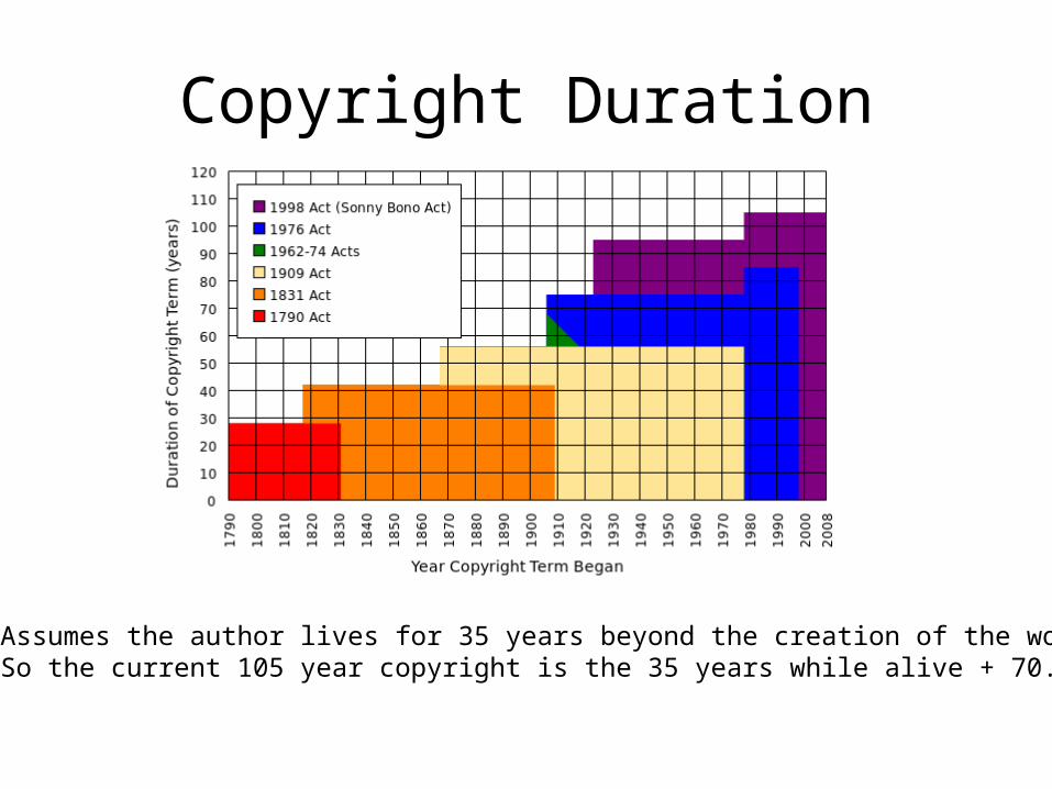
Copyright Duration
Assumes the author lives for 35 years beyond the creation of the work.So the current 105 year copyright is the 35 years while alive + 70.