market equilibrium in the presence of green consumers and
TRANSCRIPT

Dipartimento di Scienze Economiche Università degli Studi di Firenze
Working Paper Series
Dipartimento di Scienze Economiche, Università degli Studi di Firenze Via delle Pandette 9, 50127 Firenze, Italia
www.dse.unifi.it The findings, interpretations, and conclusions expressed in the working paper series are those of the authors alone. They do not represent the view of Dipartimento di Scienze Economiche, Università degli Studi di Firenze
Market Equilibrium in the Presence of Green Consumers and Responsible
Firms: a Comparative Statics Analysis
Nicola Doni and Giorgio Ricchiuti
Working Paper N. 07/2011 February 2011

Stampato in proprio in Firenze dal Dipartimento Scienze Economiche (Via delle Pandette 9, 50127 Firenze) nel mese di Febbraio 2011,
Esemplare Fuori Commercio Per il Deposito Legale agli effetti della Legge 15 Aprile 2004, N.106

Market Equilibrium in the Presence of GreenConsumers and Responsible Firms: a Comparative
Statics Analysis
May, 2011
Abstract
This paper analyzes how the interaction between green consumers andresponsible firms affects the market equilibrium. The main result is thata higher responsibility by both producers and consumers can have differ-ent impacts on the efficiency of the firms’ abatement activity, depending onthe nature of the cleaning costs. When the abatement costs are fixed, theefficiency of the clean-up effort is always increasing in their degree of re-sponsibility. On the other hand, when the abatement costs are variable, ahigher level of responsibility may reduce social welfare. Finally, the firstbest allocation is never reached, even in the presence of the highest crediblelevel of responsibility of both consumers and producers.
Key words: Green Consumers, Corporate Social Responsibility, Vertical Differentiation.
J.E.L. Classification: D62, L13, L21.
1

1 IntroductionIn the late years a growing body of the environmental economics literature hasbeen devoted to the analysis of the so called third generation instruments for thecontrol of pollution. Indeed, the classic command and control approach can besubstituted, or integrated, not only by economic instruments (i.e. taxes, subsidiesand tradable permits) but also by the voluntary market choices of environmentallyaware agents.1 However, the current debate is far from a complete understandingof the actual capabilities of both individual and firm responsibility as a means toeffectively promote environmental protection (see Bénabou and Tirole, 2010).
In many sectors firms try to increase their market share by advertising theirproduction as environment-friendly. As noted by Kotchen (2005) and Besleyand Ghatak (2007), environment-friendly goods can be viewed as impure publicgoods, in which private and public characteristics are bundled together. As em-phasized by Bagnoli and Watts (2003), the form of this bundling can be explicitor implicit. The former corresponds to situations in which firms improve the envi-ronmental quality of the good they provide and, consequently, they increase theirmarginal costs of production. The latter corresponds to situations in which firmssustain environmental programs whose benefits and costs are not proportional totheir sales.
There is a large evidence that many consumers are willing to pay a price pre-mium to purchase environment-friendly goods. The premium paid represents aform of voluntary contribution to the provision of a public good. In the economicliterature there are different ways to reconcile this behavior with the traditionalassumption of self-interested agents. A first attempt is based on the assumptionthat green consumers obtain a direct utility by the environmental qualities of thegoods they buy. In this view green consumers derive a warm glow from theirresponsible action (Andreoni, 1990), due to social approval or to their internalmoral motivation. On the other hand, we could think that green consumers be-have as conditional cooperator, who accept to sacrifice their utility conditionalon expectations that others will do the same. Indeed, other authors (e.g. Ostrom,2000) emphasized that in the presence of social dilemmas, if all the individualsseek to maximize their egoistic interest, they are unavoidably trapped in a subop-timal equilibrium. For this reason truly rational agents can choose to switch tomore refined choice criteria. We follow such kind of opinion and for this reasonin our model we assume that responsible citizens maintain the same kind of pref-
1See Khanna, 2001, for a good survey on this historical evolution.
2

erences, but adopt choice criteria that do not coincide with the maximization oftheir pay off. Coherently with this view, we consider the social welfare as the sumof agents’ pay offs and not as the sum of their objective functions representingtheir choice criteria.
The economic literature traditionally has analyzed the green consumers phe-nomenon in the framework of vertically differentiated markets. A first group ofpaper focused on how the presence of green consumers interacts with the optimalenvironmental policy (see Arora and Gangopadhyay, 1995; Cremer and Thisse,1999; Moraga-Gonzalez and Padron-Fumero, 2002; Bansal and Gangopadhyay,2003; Lombardini-Riipinen, 2005). A second group dealt with the impact of ahigher consumers’ consciousness on the market equilibrium and the associatedsocial welfare. Frequently the results of these models warn against a naive confi-dence in consumers’ responsibility as a solution to environmental problems. In-deed, rarely the market equilibrium in the presence of green consumers approx-imates the maximization of social welfare (see Eriksson, 2004; Conrad, 2005).Moreover, some authors showed that it cannot be taken for granted that a higherlevel of consumers’ responsibility is always associate to less pollution and higherwelfare2 (Rodriguez-Ibeas, 2007; Garcia-Gallego and Georgantzis, 2009).
Our paper can be considered as an extension of the vertically differentiatedduopoly put forward by Garcia-Gallego and Georgantzis (2009). They assumethat consumers have a different willingness to pay (hereafter WTP) for "clean"products and they study how an increase in their aggregate WTP affects the marketequilibrium. As far as the production technology is concerned, they assume thatthe costs and the benefits of the abatement activity are increasing and convex inthe level of clean-up and independent of the level of production. This assumptioncovers the case in which firms devote lump-sum expenditures to environmentalprotection activities not directly associated to their production of the private good.However there are cases in which the benefits and the costs of the abatement activ-ity are proportional to the quantity produced, as happens when firms improve theenvironmental quality of their production process.3 So a first extension consistsin repeating their analysis with variable costs.
Moreover, the main novelty of our paper is that we allow firms to choose their
2Similar conclusions are reached in a different framework by Calveras et al. (2007). Theyconsider a model in which citizens first vote the minimum environmental standard and then buya good produced in perfectly competitive markets. According to their analysis, a higher level ofactivism in the society may imply a higher level of pollution.
3Many existing models adopt this assumption. See for instance Cremer and Thisse (1999),Eriksson (2004), Lombardini-Riipinen (2005), Conrad (2005) and Rodriguez-Ibeas (2007).
3

market strategy in accordance with an objective function that may not coincidewith profit maximization. Indeed, in some markets, especially when the goodtraded is an impure public good, we can observe competition between firms withdifferent aims: standard for profit firms may compete with non-profit firms, whosemain objective is the maximization of the positive externality associated to theirproduction.4
Recently many firms spend a lot of efforts in order to persuade consumers thattheir behavior is socially responsible. However, there is not a general consensuswith regard to the exact concept of corporate social responsibility (CSR). We re-port two polar definitions that can appear in sharp contrast.5 According to a firstpoint of view, a firm is socially responsible when it takes environment-friendlyactions not required by law. In this light, CSR can be defined without any regardneither to the motivation of the firm’s choices nor to the impact of such choices onthe firm’s profit. From a different point of view, other authors believe that a firm istruly responsible only when it sacrifices its profit, at least in part, in order to carryout some social objective. Baron (2001) names the first behavior as strategic CSRand the second one as altruistic CSR.
In all the existing models regarding the influence of green consumers on themarket equilibrium, firms are assumed to behave as standard profit maximizers.Consequently the current literature explores only the effect of the interaction be-tween green consumers and firms engaged in strategic CSR. We propose a moregeneral approach in which firms’ objective function weighs together both profitand the social impact of their actions. In this view, firms’ degree of CSR can beinterpreted as the relative weight they assign to the second objective. Our purposeis to study the market equilibrium in the presence of green consumers and firmsengaged in altruistic CSR. More specifically this work aims at analyzing:
1. whether a higher level of responsibility of both consumers and producers isalways associated to a more efficient result in terms of pollution control;
2. whether a full responsibility of both producers and consumers is sufficientto attain the first best level of pollution.
The remaining part of the paper is organized as follows: in Section 2 wepresent the general model and introduce the concepts of green consumers and
4Becchetti and Huybrechts (2007) interpret in this way the Fair Trade sector.5An interesting debate over this issue can be found in the first volume of the Review of Envi-
ronmental Economics and Policy. In particular, see Lyon and Maxwell (2008) and Reinhardt et al.(2008).
4

responsible firms. In Section 3 we characterize the market equilibrium in the casein which the costs and the benefits of the cleaning technology are fixed (i.e.: in-dependent of the quantity produced). In Section 4 we extend the same kind ofanalysis to the alternative case in which the costs and the benefits of clean-up areassumed to be proportional to the quantity produced. Section 5 concludes.
2 The general model
2.1 The technologyThere is a physically homogeneous good, whose production generates pollution.The production costs depend on both the quantity produced, x, and the level ofthe abatement activity, e. Formally, the cost function for a generic firm i is:
Ci(ei) =k
2e2ix
γi , ∀i = 1, ..., n, (1)
where k is a constant and γ indicates how the quantity produced affects the abate-ment costs. Specifically, γ can assume two values: zero when the abatement costsare fixed, and one when these costs are variable.
The total emissions for a single firm are:
Yi(ei) = exi − eixγi , ∀i = 1, ..., n; (2)
e is the unitary level of emissions without clean-up activity. We assume that whenthe abatement costs are fixed, γ = 0, then the clean-up activity of a generic firmi is independent of xi. In this case, according to the definition introduced byBagnoli and Watts (2003), the private provision of the public good "abatement" isonly implicitly linked to sales of the private good. On the other hand, when theabatement costs are variable, γ = 1, the clean-up activity of firm i is proportionalto xi. This case corresponds to a situation in which the provision of both publicand private good are explicitly linked. Finally, let us define Y =
∑ni=1 Yi the
aggregate emissions.
2.2 The market actors and the social welfareOn the demand side there is a unit mass of consumers that are interested in buyingonly one unit of the good. Their utility function is:
U = V − p− ρY, (3)
5

where V is the (homogeneous) gross utility of consuming one unit of the product,p is its price and ρ is the marginal disutility that each consumer associates to thenegative externality stemming from pollution. We assume that ρ is distributedaccording to F (ρ) over the support
[ρ, ρ], where F (ρ) = 0 and F (ρ) = 1. As a
consequence, the social benefits of the clean-up activity is equal to ρTET whereET =
∑ni=1 eix
γi is the total abatement and ρT =
∫ρdF (ρ) is its marginal social
benefit. We assume that V is higher than e and consequently the production of thisgood is always socially efficient, in the sense that the associated social benefits arehigher than the correspondent social costs.
On the supply side there are n firms which share the common technology.Imagine that a generic firm i adopts a level of abatement ei, charges a price equalto pi and sells to a market share xi. In such case its profit is:
πi = pixi −k
2e2ix
γi , i = 1, ..., n. (4)
We assume that every consumer buys the product of one firm; consequently,∑ni=1 xi = 1. The social welfare W is defined as the sum of consumers’ surplus
and firms’ profit. In a generic market allocation it is equal to:
W = V − ρT e+n∑i=1
[ρT ei −
k
2(ei)
2
]xγi . (5)
It is worth noting that W corresponds to the difference between the socialbenefits and the total costs associated to the aggregate clean-up. Consequently wecan identify the social welfare with the efficiency of the environmental protectionactivity.
The maximization of the social welfare entails that the first best level of clean-up of each firm is:
eFB =ρT
k, ∀i = 1, ..., n, (6)
which does not depend on the quantity produced. It is worth noting that whateverthe total abatement is, its cost effective allocation requires that firms’ marginalcosts coincide, implying that total abatement should be shared equally amongthem.
We assume that the environmental regulator cannot force firms to adopt a pos-itive level of clean-up. Consequently, if ρT is strictly higher than 0, then the publicgood "abatement" is too scarce and responsible citizens can choose to voluntarilycontribute to its provision by producing or consuming more environment-friendlygoods.
6

2.3 The green consumersWe assume that a share 0 ≤ β ≤ 1 of consumers’ population (labeled as green)takes into account firms’ abatement efforts in choosing which product to buy,while all the others consumers acts as (radical) free riders. We let the WTP ofgreen consumers be heterogeneous among them. Formally, a generic green con-sumer chooses a product to maximize:6
H = V − p− ρY + θe, (7)
where θ is the individual WTP for the marginal increase in firms’ abatement, as-sumed uniformly distributed in the interval
[0, θ].7 Therefore the total WTP for
more environment-friendly products, θT , is equal to βθ2
. Let us define µ as:
µ =θT
ρT=
βθ
2ρT. (8)
This ratio can be considered as an index of the social capital of the consumers’population because it represents how much their choices are driven by social ratherthan individualistic motivations. We limit the aggregate consumers’ WTP to belower than their aggregate marginal disutility of emissions, i.e. θT ≤ ρT . Giventhis assumption, it follows that 0 ≤ µ ≤ 1.
2.4 The responsible firmsFollowing Garcia-Gallego and Georgantzis (2009), we assume that on the supplyside there is the coexistence of two kinds of firms. On the one hand, a fringeof firms who provide the good without employing any clean-up activity. Giventhat they sell an homogenous product and compete à la Bertrand, they charge aprice equal to 0 (the marginal cost of production when e = 0), and they do notachieve extra profit. On the other hand, in the presence of green consumers, otherfirms can choose to employ the cleaning technology in order to differentiate theirproduct and to obtain a strictly positive profit. We assume that there are only
6We assume that each consumer takes the total emissions Y as exogenous because her individ-ual contribution to pollution is negligible.
7We choose to pay attention only to the case in which the lowest WTP is 0 in order to simplifyour analysis of the market equilibrium. Indeed, the assumption that θ = 0 ensures that only anincomplete market coverage configuration can arise in equilibrium, as shown by Liao (2008) forthe fixed costs case and by Ecchia and Lambertini (1998) for the variable costs case.
7

two firms that are able to carry out this abatement activity. We use H and L todenote the variables associated to the firms choosing the high and the low level ofabatement.
These two firms are labeled as responsible because they overcomply the ex-isting environmental regulation. As sustained by Kotchen (2009), environment-friendly innovations are frequently introduced by eco-entrepreneurs where eco-entrepreneurship can be defined as "the practice of starting new businesses inresponse to an identified opportunity to earn a profit and provide a positive en-vironmental externality". So, the assumption regarding the existence of only tworesponsible producers can be justified by noting that frequently innovation pro-cesses are driven by a limited number of firms.
We assume that responsible firms can have a different willingness to sacrificetheir profit in order to increase their clean-up. Formally, we allow them to havethe following composite objective function that weighs the maximization of theirprofit and the maximization of the positive externality associated to their abate-ment activity:
Ji =(πi)1−αi
(ρT eix
γi
)αi s.t. πi ≥ 0, i = L,H, (9)
where αi ∈ [0, 1]. When αi = 0 we have the standard case of a profit-maximizerfirm; when αi = 1 we have the opposite case of a non-profit firm who simplywants to maximize the positive impact of its clean-up under the constraint of non-negative profit.8 In general, a responsible firm i pursues two different objectivessimultaneously and αi is a parameter signaling the relative importance of the twoobjectives. More specifically, αi can be interpreted as a measure of the degree of(altruistic) CSR of firm i. As explained in De Donder and Roemer (2009), suchobjective can be interpreted as the weighted Nash bargaining solution of an ef-ficient negotiation between two different factions inside the firm: one aiming atmaximizing profit and the other aiming at maximizing the positive externality as-sociated to firm’s production. Such interpretation is correct if i) the no agreementpay-offs are (0, 0), as happens when a firm is part of the competitive fringe, thatdoes not obtain any extra-profit and does not produce any positive externality, ii)the objective function of each faction is log-concave in firm’s strategic choices ofp and e (for our case this property is proved in the technical appendix). Accordingto such interpretation, αi represents the relative bargaining power of the factionsupporting the abatement activity inside the firm i.
8We assume that when αi = 1 firm i maximizes the positive impact of its abatement activityeven if its profit is equal to 0.
8

2.5 Firms’ competitionWe model competition between the two responsible firms according to the usualframework adopted in duopoly models of vertical differentiation. There are twostages: in the first one, the two firms simultaneously choose the clean-up level,that can be defined as the (environmental) quality of their product. In the secondstage the two firms observe the choice of their competitor and simultaneouslyset the price. We know that when the lowest consumers’ WTP is equal to 0, inequilibrium arises an uncovered market configuration (see Liao, 2008, and Ecchiaand Lambertini, 1998). This means that in equilibrium a group of green consumersbuys a standard good from the competitive fringe.
The market share of each firm can be calculated by identifying θ, the consumerwhich is indifferent between the high or the low quality product, and θ, that whichis indifferent between the low or the null quality product. Straightforward algebra,using equation (7), it is easy to see that: θ = pH−pL
eH−eLand θ = pL
eL. As known,
in a vertically differentiated duopoly, the high (low) quality firm sells to greenconsumers included in
[θ, θ] ([
θ, θ])
. Then each firm’s market share is:
xH =β
θ
[θ − pH − pL
eH − eL
], xL =
β
θ
[pH − pLeH − eL
− pLeL
], x0 = 1− xH − xL, (10)
where x0 is the total quantity sold by firms of the competitive fringe.We apply the standard backward induction methodology by first analyzing the
price equilibrium and then the environmental quality equilibrium.
3 Fixed costs of clean-up
3.1 The market equilibriumIn this section we study the case of fixed costs of clean-up, i.e. γ = 0. By usingequations (4) and (9) we can specify the objective function of the responsible firmsas:
Ji =
(pixi −
k
2e2i
)1−αi(ρT ei
)αi
s.t. πi ≥ 0, i = L,H. (11)
It is worth noting that in case of fixed costs the generalization of the firms’objective function has no consequence on the price-setting stage. Indeed, at the
9

second stage the abatement activity is considered as exogenous, and so the respon-sible firms choose their price strategy in order to maximize only their revenues,whatever their degree of CSR is. So the price equilibrium can be found by solvingsimultaneously the revenue maximization of both firms. As shown in the existingliterature (Motta, 1993; Arora and Gangopadhyay, 1995), at this stage the uniqueNash equilibrium is characterized by the following equations:
p∗H = 2θeHeH − eL4eH − eL
,
p∗L = θeLeH − eL4eH − eL
,
yielding profits:
πH = 4βθe2H
(eH − eL)
(4eH − eL)2− k
2e2H ; (12)
πL = βθeHeL(eH − eL)
(4eH − eL)2− k
2e2L. (13)
In order to identify the duopolists’ maximization problem at the first stage,equations (12) and (13) are substituted in equation (11). The equilibrium levelsof clean-up corresponds to the solutions that solve simultaneously9 the followingunconstrained10 maximization problems:11
maxeH
[4βθe2
H
(eH − eL)
(4eH − eL)2− k
2e2H
]1−αH(ρT eH
)αH
;
maxeL
[βθeHeL
(eH − eL)
(4eH − eL)2− k
2e2L
]1−αL(ρT eL
)αL
.
The first order conditions require:9As explained by Motta (1993), the solutions of this system are only the candidate equilibrium
of the model. In the technical appendix we show that second order conditions hold, and conse-quently every solution represents effectively a local maximum. Moreover, we have checked thatthe firm choosing the high (low) quality has no incentive to "leapfrog" the rival firm and itselfproduce the lowest (highest) quality.
10We neglect the constrain that the firms’ profit must be positive as we will verify that suchcondition is always satisfied in equilibrium.
11We use αH and αL to indicate the degree of CSR of the firms producing the high and the lowlevel of clean-up. However, it is important to emphasize that we do not restrict the relative size oftheir degree of CSR.
10

∂JH∂eH
= 0⇔ βθ4e3
H − (3 + 2αH)e2HeL + (2− αH)eHe
2L
(4eH − eL)3=
2− αH8
keH ; (14)
∂JL∂eL
= 0⇔ βθ4e3
H − (7− 2αL)e2HeL + αLeHe
2L
(4eH − eL)3=
2− αL2
keL. (15)
In order to study whether firms’ abatement activities are strategically substi-tutes or complements we have to investigate the sign of the following cross deriva-tives:
∂2JH∂eH∂eL
= 4βθ−8αHe
2H + (10− 12αH)eHeL + (2− αH)e2
L
(4eH − eL)4; (16)
∂2JL∂eL∂eH
= βθeL(16− 8αL)e2
H + (14− 12αL)eHeL − αLe2L
(4eH − eL)4. (17)
Straightforward, the cross derivatives of each firm’s objective function is de-creasing in its own degree of CSR. However, the cross derivative of firm L (eq.17) is always positive (given that αL ≤ 1): in equilibrium the optimal abatementfor the low quality firm is always increasing in the abatement chosen by its rival.Conversely, the cross derivatives of firmH (eq. 16) is strictly positive for αH = 0,while is strictly negative when αH = 1. Hence, the best response of the high qual-ity firm can be both increasing and decreasing in the abatement level chosen byits rival, depending on its own degree of CSR (and on the equilibrium levels offirms’ abatement).
Following the definition of Bulow et al. (1985), if αH is quite low, then eHand eL are strategic complements, while for higher values of αH , we have neitherstrategic complementarity nor strategic substitutability at the second stage becausethe slopes of the two reaction functions have different sign.
The solutions of the system given by equations (14) and (15) can be foundmaking the ratio between them. We obtain:12
4(2− αH)λ3 − (46− 20αL − 7αH + 2αLαH)λ2+
+ (24− 10αL + 16αH − 9αLαH)λ− 4(2− αL)(2− αH) = 0,
12This equation is a generalization of equation (7) of Motta (1993, p. 117) to the case in whichfirms aim at maximizing not only their profit but also the positive externality implicitly associatedto their production.
11

where λ is equal to eHeL
. λ can be interpreted as the degree of (environmental)differentiation. This equation has a unique acceptable solution λ∗ = g(αH , αL).In Figure 1 we show the three dimensional plot of λ∗. It is monotonically in-creasing (decreasing) in αH (αL), ∀αH , αL ∈ [0, 1]: hence, the higher the degreeof CSR of the firm H (L) the higher (lower) the environmental differentiation.It’s worth noting that λ∗ has a maximum in g(1, 0) = 8, 6164 and a minimum ing(0, 1) = 2, 7452.
Figure 1: λ∗ = g(αH , αL)
Substituting eH with λ∗eL in (15) we achieve the equilibrium level of clean-upof both firms as a function of λ∗, αL, β, θ, k:
e∗L =2βθ
(2− αL)k
λ∗[4(λ∗)2 − (7− 2αL)λ∗ + αL]
(4λ∗ − 1)3;
e∗H =2βθ
(2− αL)k
(λ∗)2[4(λ∗)2 − (7− 2αL)λ∗ + αL]
(4λ∗ − 1)3.
By recalling and rearranging the equations (6) and (8) we obtain:
e∗L =4µλ∗[4(λ∗)2 − (7− 2αL)λ∗ + αL]
(2− αL)(4λ∗ − 1)3eFB; (18)
e∗H =4µ(λ∗)2[4(λ∗)2 − (7− 2αL)λ∗ + αL]
(2− αL)(4λ∗ − 1)3eFB. (19)
12

Trivially, if all consumers are radical free riders (i.e.: µ = 0), firms will notemploy a cleaning technology, whatever their objective function is. It’s worthnoting that in this model in order to have an abatement activity in equilibrium thepresence of green consumers is both necessary and sufficient. On the other hand,the mere existence of responsible firms is not sufficient.
Lemma 1. In the presence of green consumers (i.e.: if µ > 0), ∀αH , αL, µ ∈[0, 1], 0 < e∗L < e∗H < eFB.
Proof. In Figure 2 we report the ratio13 eH over eFB calculated by means of equa-tion (19). It can be easily seen that it is always positive but less than 1. Moreover,given that λ∗ is always strictly higher than 1, e∗L is always less than e∗H for µ > 0.
Figure 2: e∗H/eFB
This lemma allows us to conclude that, even if consumers and producers werefully responsible, the market equilibrium will not correspond to the first best al-location: both the responsible firms never adopt an efficient level of clean-up.Moreover the allocation of the aggregate abatement is not cost-effective becausein equilibrium the two responsible firms never adopt the same level of clean-upand so their marginal costs differ.
13Figure 2 is plotted under the assumption that µ = 1, so it indicates the maximum values ofthe ratio eH over eFB .
13

In order to analyze how the degree of responsibility of both consumers andproducers affects the overall efficiency of the abatement activity we can now con-duct some comparative statics. Note that given equations (18) and (19) there is apositive relationship between the social capital index and the equilibrium level ofclean-up of both the responsible firms.
Lemma 2. In the presence of green consumers (i.e.: if µ > 0):
1. e∗L is monotonically increasing in αL and αH , ∀αH , αL ∈ [0, 1];
2. e∗H is monotonically increasing in αH , while it is monotonically increasing(decreasing) in αL if αH is close to 0 (1). For intermediate values of αH ,eH is not monotone in αL;
3. ET∗ = e∗H+e∗L is monotonically increasing in αL and αH , ∀αH , αL ∈ [0, 1].
Proof. The influence of the degree of CSR of both the responsible firms on theirequilibrium levels of abatement are proved by means of the contour plots shownin Figure 3. The left-hand side shows that e∗L has iso-curves negatively sloped andthat it reaches its maximum value in the point (αH = 1, αL = 1). This meansthat e∗L is monotone increasing in both αH and αL. On the other hand, the centralcontour plot shows that the iso-curve of e∗H are decreasing in correspondence oflow values of αH and increasing for high values of αH . Moreover, e∗H reachesits maximum value in correspondence of the point αH = 1, αL = 0. This provethat a higher αH always implies a higher e∗H , while the influence of αL on e∗Hdepends on the value of αH . Finally, the right-hand side shows that the sum offirms’ abatement activities in equilibrium is monotone increasing in both αH andαL. Indeed, the iso-curves are negatively sloped and the maximum is reached inthe point (αH = 1, αL = 1).
Therefore increments in the degree of responsibility of a firm always entails anincrease of its own abatement activity. On the other hand increments in the degreeof responsibility of the rival firm may not have a clear-cut effect for both firms.Indeed, it is always true that the higher αH , the higher e∗L, while an increment ofαL may both increase and decrease e∗H , depending on the level of αH . This resultis due to the different sign that the cross derivative of JH can assume. As seenabove, when firm H carries out a sufficiently high (low) degree of CSR, then itsbest response is decreasing (increasing) in the level of clean-up of firm L. As aconsequence, given that an increment of αL increases e∗L, we have that when αH
14

Figure 3: Contour Plot of e∗L and e∗H
Note: the lighter colors are associated with higher values.
is sufficiently high (low) e∗H is decreasing (increasing) in αL. However, the totallevel of abatement is monotonically increasing in the degree of CSR of each firm.
3.2 The social welfareIn the case of fixed costs of clean-up, the social welfare defined in equation (5)can be rewritten as:
W =∑i=H,L
ρT e∗i −k
2(e∗i )
2. (20)
Proposition 1. The social welfare is monotonically increasing in µ, αL and αH ,∀ µ, αH , αL ∈ [0, 1].
Proof. We can write the variation of W with respect to a generic exogenous pa-rameter z as:
∂W
∂z=∑i=H,L
(ρT − ke∗i )∂e∗i∂z
. (21)
Given Lemma 1, e∗i < eFB ⇔ ρT − ke∗i > 0. Therefore, the sign of thederivatives of the social welfare with respect to an exogenous parameter will de-pend only on how such parameter affects the equilibrium level of clean-up of bothfirms. If ∂e∗i
∂zhas the same sign, ∀i = L,H , then also ∂W
∂zwill have that sign.
15

Therefore, given equations (18) and (19) and Lemma 2, the social welfare is ev-erywhere increasing in µ and αH . As far as αL is concerned, rearranging equation21 we obtain:
∂W
∂z= (ρT − ke∗L)
∂ET ∗
∂z+ k(e∗H − e∗L)
∂e∗L∂z
. (22)
Applying Lemma 2 to formula 22 we can conclude that the social welfare ismonotone increasing also in αL. The following contour plot (Figure 4) confirmsthat the social welfare has its global maximum in (αH = 1, αL = 1).
Figure 4: Contour Plot of W (αH , αL)
This result is in line with Garcia Gallego and Georgantzis (2009), who hadalready shown that, in the uncovered market configuration, the social welfare isincreasing in consumers’ WTP. However, in this paper we show that the socialwelfare is also increasing in the degree of CSR of both the responsible firms.
Corollary 1. The highest social welfare is attained when µ = 1, αL = 1 andαH = 1, but it does not correspond to the first best solution.
Proof. Proposition 1 ensures that the maximum welfare associated to the marketequilibrium is reached when both µ, αL and αH have their maximum value. Insuch case, the social welfare calculated by means of equation (20) is equal to
16

0, 4366 (ρT )2
k. However, if the level of abatement of both the responsible firms
was ρT
k, i.e. its first best level, then the social welfare would be equal to (ρT )2
k.
Therefore in this case the social welfare attained in equilibrium is only the 43, 66%of its first best level.
Therefore, the market equilibrium never achieves the first best solution, evenif both consumers and producers behave as fully responsible agents. The inef-ficiency of the market equilibrium is due to two different reasons: firstly, theclean-up of both the responsible firms is always lower than the first best level andconsequently total abatement is below its optimal level. Moreover, the allocationof total abatement is not cost effective because it is not equally shared betweenthe two responsible firms, whatever their degree of altruistic CSR is (both thesefacts are emphasized in Lemma 1).
To sum up, when the clean-up activity of the responsible firms is only implic-itly linked to their production, the efficient level of the abatement is never reachedin equilibrium (Corollary 1). However, an increase of both firms’ CSR and con-sumers’ WTP have always a positive effect on the social welfare (Proposition 1).In the next section we shall show that even this result is not guaranteed when theclean-up activity is explicitly associated to the production level (i.e. when bothbenefits and costs of the cleaning technology are variable).
Proposition 2. Let us assume that αH = α′L > αL = α′H; then W (αH , αL) >W (α′H , α
′L), ∀αH , αL ∈ [0, 1].
Proof. Let us analyze the contour plot of the Welfare (Figure 4). It is straightfor-ward that if we consider both a point such that αH > αL and its symmetric pointwith respect to the 45◦ line, the former is always associated to a higher socialwelfare than the latter.
The existing literature regarding vertically differentiated duopolies has alreadystressed the existence of two asymmetric and specular Nash equilibria at the qual-ity stage. However, in the present model these two equilibria are no more specular(if αH 6= αL) given the differences in the firms’ objective functions. Proposition 2states that the social welfare is always higher in the equilibrium in which the highquality firms is at the same time the firm with the highest degree of CSR.
Thanks to Propositions 1 and 2 we can compare a standard duopoly, wherethe firms are both profit maximizers, with a mixed duopoly, where a non-profitproducer competes with a profit maximizer firm. When the costs of the abatementactivity are only implicitly linked to the production level, then the presence of a
17

non-profit firm is always welfare improving, and from the social welfare stand-point it is preferable the equilibrium in which the non-profit firm carries out thehighest level of clean-up.
4 Variable costs of clean-up
4.1 The market equilibriumIn this section we study the case of variable costs of clean-up, i.e. γ = 1. Firms’objective function is:
Ji =(πi)1−αi
(ρT eixi
)αi , i = L,H, (23)
where:
πi =
(pi −
k
2e2i
)xi, i = L,H, (24)
and the market shares of each firm are still given by (10). In this case the prices af-fect not only firms’ profit but also the size of their positive externality. Therefore,equilibrium prices are now dependent on the degree of CSR of both firms.
By computing the first derivatives of JH and JL with respect to prices and thensolving the system we obtain the following equations for the equilibrium prices:
p∗H =eH[(2− αL)ke2
H + (1− αH)ke2L + 2θ(1− αH)(2− αL)(eH − eL)
]2[(2− αH)(2− αL)eH − (1− αH)(1− αL)eL]
,
p∗L =eL[(1− αL)ke2
H + (2− αH)keLeH + 2θ(1− αH)(1− αL)(eH − eL)]
2[(2− αH)(2− αL)eH − (1− αH)(1− αL)eL],
yielding profits:
πH = (1− αH)(eH − eL)x2H
θ
β, (25)
πL = (1− αL)(eH − eL)eLeHx2L
θ
β, (26)
where:
18

xH =βeH
[(2− αL)(2θ − keH)− keL)
]2θ[(2− αH)(2− αL)eH − (1− αH)(1− αL)eL]
, (27)
xL =βeH
[(1− αH)(2θ − keL) + keH)
]2θ[(2− αH)(2− αL)eH − (1− αH)(1− αL)eL]
. (28)
We can now include equations (25) and (26) in the generic equation (23) andderive the first order conditions of the first stage obtaining the following systemof equations:
∂JH∂eH
= 0⇔ (2− αH)(eH − eL)∂xH∂eH
+eH − αHeL
eHxH = 0; (29)
∂JL∂eL
= 0⇔ (2− αL)(eH − eL)eLeH
∂xL∂eL
+eH − 2eL + αLeL
eHxL = 0. (30)
Moorthy (1988) has already shown that when vertically differentiated firmsbehave as profit maximizers, their reaction functions are both positively slopedand so their quality choices are strategic complements. However, it is easy tocheck that if the high quality firm is a non-profit firm, i.e. when αH = 1, itsbest response function is negatively sloped14 while the best response function offirm L is still positively sloped. Therefore we may not record neither strategiccomplementarity nor strategic substitutability, as in the fixed costs case.
The system given by equations (29) and (30) can have at maximum one ac-ceptable solution (i.e.: such that e∗H ≥ e∗L). When one solution exists, such so-lution corresponds to the equilibrium levels of marginal clean-up of both firms15,which depends on the parameters αH and αL. The solutions in the closed formare not analytically feasible. However, some clear results emerges when one ofthe duopolists is a non-profit firm and it produces either the high-quality or thelow-quality good.
Proposition 3. If αL = 1, then at the first stage no Nash equilibrium exists.
14Indeed, in such case the cross derivative of the objective function of firm H is equal to− βk
2θ(2−αL).
15In the technical appendix it is shown that in correspondence of the unique acceptable solutionsecond order conditions hold also in the case of variable costs. However, not all the candidatesolutions are valid because, as reported in the technical appendix, in some cases some firm has anincentive to leapfrog the "equilibrium" level of marginal abatement of its rival.
19

Proof. In this case the market shares of the responsible firms can be rewritten bysubstituting αL = 1 in formula (27) and (28). We obtain:
xH =β(2θ − keL − keH)
2θ(2− αH), (31)
xL =β[(1− αH)(2θ − keL) + keH ]
2θ(2− αH). (32)
The derivatives of JL with respect to eL is equal to:
∂JL∂eL
= eL∂xL∂eL
+ xL = 2(1− αH)(θ − keL) + keH (33)
From equation (31) we can deduce that xH ≥ 0⇔ keL ≤ θ. This implies thatequation (33) is always strictly positive. Consequently, at the first stage the firmL would choose eL = eH , the maximum level of marginal abatement under theconstraint that eL must be weakly lower than eH . On the other hand, if αH < 1,the firm H always would choose eH > eL, because if eH = eL its profit is equalto 0.
Therefore, when one of the two responsible producers is a non-profit firm,there is no equilibrium in which it chooses the low level of marginal abatement.Indeed, in such case the firm L would mimic the choice of its competitor, whilethe firm H would prefer level of marginal abatement strictly higher than the levelof its rival.
As a consequence, in the presence of a non-profit firm, the only Nash equilib-rium can be characterized by substituting αH = 1 in equations (29) and (30).
Lemma 3. If β > 0, θ > 0, and αH = 1, then in equilibrium:
1. e∗L is monotonically increasing in both θ and αL, decreasing in k and inde-pendent of β;
2. x∗L is monotonically increasing in both β and αL and independent of both θand k;
3. e∗H is monotonically increasing in θ, decreasing in both k and αL and inde-pendent of β;
4. x∗H is monotonically increasing in β, decreasing in αL and independent ofboth θ and k;
20

5. ET∗ = e∗Hx∗H + e∗Lx
∗L is monotonically increasing in both β and θ and
decreasing in both k and αL.
Proof. Note that if β > 0, θ > 0, αH = 1 and αL ∈ [0, 1) then the solution of thesystem identifies the following equilibrium levels of marginal abatement:
e∗L =2(2− αL)
9− 8αL + 2α2L
θ
k; (34)
e∗H =2(2− αL)2
9− 8αL + 2α2L
θ
k. (35)
Substituting these solutions in equations (27) and (28), the following equilib-rium market shares are achieved:
x∗L =β(2− αL)
9− 8αL + 2α2L
(36)
x∗H =β(2− αL)2
9− 8αL + 2α2L
(37)
Straightforward algebra the parameters β, θ and k affect e∗L, x∗L, e∗H , x∗H andET∗ in the way stated in the lemma. As far as the impact of the degree of CSRof the low-quality firm on firms’ marginal abatement choices and on their marketshares, the results stated in the proposition stem from the following derivatives:∂e∗L∂αL
= 2θβk
∂x∗LαL
> 0; ∂x∗L∂αL
= β2α2
L−8αL+7
(9−8αL+2α2L)2
> 0; ∂e∗H∂αL
= 2θβk
∂x∗HαL
< 0; ∂x∗H∂αL
=
−β 2(2−αL)
(9−8αL+2α2L)2
< 0; ∂ET∗
∂αL= 4βθ
2k2αL−4
(9−8αL+2α2L)4
< 0.
In the presence of a non-profit firm, the unique Nash equilibrium is charac-terized by the fact that the other firm always adopts the lowest level of marginalabatement. Moreover, the higher the weight assigned by the low quality firm to itsCSR, the higher its positive externality is. However, this effect is counterbalancedby the reduction of the positive externality of the high quality firm. This result iscoherent with the slope of the best response function of firmH . If firm L becomesmore careful with the environmental impact of its production, it will increase itslevel of abatement, but at the same time, it will reduce its mark-up, increasingits supply. On the other hand, firm H cannot reduce its price without reducingits level of clean-up because it always charges a price equal to its marginal costs.Hence, firm H finds it convenient to decrease its level of abatement in order to
21

Figure 5: Nash equilibrium existence
limit the reduction of its market share. The last statement shows us that the aggre-gate effect of an increase in αL entails a reduction of the total abatement.
More general results regarding the market equilibrium in the presence of tworesponsible firms can be obtained by means of numerical simulations. The shadedregion of Figure 5 identifies the set of couples (αH , αL) in which a Nash equi-librium (in pure strategies) does to exist: firm H would have an incentive toleapfrog16 firm L by choosing a level of abatement lower than e∗L(αH , αL) in orderto increase its market share and its total abatement. Consequently, at the first stagewe can have zero, one or two Nash equilibria, depending on the weight that boththe responsible firms assign to their profit. Indeed, making the symmetry of theshaded region with respect to the bisectrix we can identify three different regions.When the shaded region and its symmetric region coincide no Nash equilibriumexists. For all the other couples of values of (αi, αj) contained in the shaded re-gion only a Nash equilibrium exists, in which αH > αL. Finally, for the couplesof (αi, αj) contained neither in the shaded region nor in its symmetric counterpart,two Nash equilibria exist.
Hence, if both firms assign a high weight to the positive externality associatedto their own production, the outcome of their strategic interaction is unpredictable.However, when a Nash equilibrium exists, we can analyze through numerical cal-
16The numerical calculations are available upon request.
22

culations how the market equilibrium is affected by consumers’ and firms’ degreeof responsibility. It is worth noting that both e∗L and e∗H are linearly increasing inθk
and independent of β, while both x∗L and x∗H are linearly increasing in β and in-dependent of both θ and k. As far as the impact of firms’ degree of responsibilityon market equilibrium we resume the main observations in the following lemma:
Lemma 4. When at least a Nash equilibrium exists, the following properties hold:
1. e∗L is monotonically increasing in αL, while it is increasing (decreasing) inαH only when αL is sufficiently low (high). For intermediate values of αL,e∗L is (almost) constant. x∗L is monotone increasing in αL and monotone de-creasing in αH . Finally, e∗Lx
∗L is monotone increasing in αL and monotone
decreasing in αH .
2. e∗H is monotonically increasing (decreasing) in αH only when αL is suf-ficiently low (high). For intermediate values of αL, e∗H is first increasingand then decreasing. At the same time, e∗H is monotonically increasing (de-creasing) in αL only when αH is sufficiently low (high). For intermediatevalues of αH , e∗H is first decreasing and then increasing. x∗H is monotone in-creasing in αH and monotone decreasing in αL. Finally, e∗Hx
∗H is monotone
increasing in αH and monotone decreasing in αL.
3. ET∗ = e∗Hx∗H + e∗Lx
∗L is monotone increasing (decreasing) in αH if αL is
sufficiently low (high) and monotone increasing (decreasing) in αL if αH issufficiently low (high).
4. λ∗ = e∗H/e∗L is always monotone decreasing in αL while it is monotone
decreasing in αH only if αL is sufficiently high. When αL is low, λ∗ is firstincreasing and then decreasing in αH .
Proof. See the 3D plots in Figure 6.
The equilibrium levels of marginal abatement are affected in several ways byfirms’ degree of responsibility. At the same time, both firms’ market share andtotal abatement are always increasing in their own degree of CSR, and decreas-ing in the degree of responsibility of the rival firm. The overall impact on theaggregate level of clean-up is ambiguous: an increase in the CSR of firm L (H)can either increase or decrease the aggregate clean-up depending on the CSR offirm H (L). Finally, an increase in the degree of responsibility of firm L makes theallocation of the abatement activity more cost effective (i.e. it decreases the value
23

of λ∗), while an increase in the degree of responsibility of firm H does not have aclear-cut effect on λ∗.
Lemma 5. When at least a Nash equilibrium exists, e∗H S eFB and e∗L S eFB,depending on the specific values of θ, αL, αH . At the same time, ρT − k
2e∗i > 0,
∀i = L,H , ∀θ, αL, αH .
Proof. In Figure 6 we set parameters as follows: β, θ and k are equal 1, andthere are couples (αH , αL) for which e∗H and/or e∗L are higher than 0.5. As aconsequence, given the linear proportionality to θ, when maximum consumers’WTP is close to its maximum value (i.e. 2ρT ) both the responsible firms mayexert a level of abatement higher than the first best level (i.e. ρT
k). At the same
time, the equilibrium levels of clean-up do not assume a value higher than θk.
Hence, the inequality contained in the lemma follows.
Despite the fixed costs case, when the costs are variable in equilibrium bothfirms may choose to exert an inefficiently high level of abatement (i.e. higherthan the first best level). Hence, the statements of Lemma 4 and 5 do not helpus to draw any clear inference with regard to the influence of a higher degree ofresponsibility on the social welfare. Indeed, a higher green consumers’ WTP al-ways increases the aggregate abatement, but it may induce the responsible firms toadopt an inefficiently high level of marginal abatement. At the same time, an in-crease in the degree of CSR of one firm has not a clear-cut effect on the aggregateabatement and on the cost-effectiveness of the allocation of such activity.
4.2 The social welfareIn the case of variable costs of clean-up, the social welfare defined in equation (5)can be rewritten as:
W =∑i=H,L
[ρT e∗i −
k
2(e∗i )
2
]x∗i . (38)
Proposition 4. The social welfare is monotone increasing in β while its partial(first) derivative with respect to θ is never monotone.
Proof. The variation of W with respect to a generic exogenous parameter z is:
∂W
∂z=∑i=H,L
[(ρT − ke∗i )x∗i
∂e∗i∂z
+ (ρT − k
2e∗i )e
∗i
∂x∗i∂z
].
24

Consequently, ∂W∂β
is surely positive given that ∂e∗i∂β
= 0, (ρT − k2e∗i ) > 0 (see
Lemma 5) and ∂x∗i∂β
> 0, ∀i = L,H .
Given that ∂x∗i
∂θ= 0 and ∂2e∗i
∂θ2= 0 we obtain that:
∂2W
∂θ2= −k
∑i=H,L
x∗i
(∂ei∂θ
)2
< 0
Hence, W is concave in θ. Furthermore, as ∂e∗i∂θ
> 0 and ∂x∗i∂θ
= 0, we can notethat the sign of ∂W
∂θdepends on the sign of (ρT − ke∗i ), ∀i = L,H . Consequently,
when θ is close to 0 (2ρT ) both e∗H and e∗L are lower (higher) than eFB and W isincreasing (decreasing) in θ. Therefore, W is never monotone in θ.
As far as the pattern of W with respect to αL and αH , it is not feasible toderive analytical results. Using numerical simulations, we show that W can beboth increasing and decreasing in firms’ CSR, depending on the specific values ofαL, αH and θ (see Figure 7).
Therefore, in the variable costs case, the impact of αH and αL on the socialwelfare depends crucially on their values and on the value of θ. In some cases ahigher degree of responsibility of one firm can harm the social welfare. For in-stance, the social welfare turn out to be monotonically decreasing in αL when αHis very high and θ is very low. At the same time, the social welfare is monotoni-cally decreasing in αH when αL is very low and θ is very high.
Proposition 5. The highest social welfare is attained when β = 1, θ ' 1, 463ρT ,αH = 1 and αL ' 0, 85, and it does not correspond to the first best solution.
Proof. The maximum of W can be obtained through numerical calculations. Incorrespondence of such values W = 0.33783 (ρT )2
k. If all the existing firms could
adopt a level of abatement equal to the first best level the social welfare wouldbe equal to 0.5 (ρT )2
k. Therefore, when the abatement cost are explicitly linked to
sales, the maximum social welfare achievable in equilibrium is only the 0, 67% ofits first best level.
Proposition 6. If θ is sufficiently high, social welfare is higher in a standardduopoly than in a mixed duopoly.
Proof. Thanks to Figure 5 we know that in the presence of a non-profit firm andof a profit-maximizing a unique Nash equilibrium exists, in which the formerchooses the high level of abatement and the latter the low level. Observing the
25

third graph in Figure 7 we can note that when θ is very high, W (0, 0) > W (1, 0).Therefore social welfare is higher in a standard duopoly (i.e. in the presence oftwo profit-maximizing firms) than in a mixed duopoly (i.e. in the presence a non-profit firm and a profit-maximizing firm)
Proposition 7. Let us assume that αH = α′L > αL = α′H . There are cases inwhich W (αH , αL) < W (α′H , α
′L).
Proof. Observing the third graph in Figure 7 we can note that when θ is veryhigh, the social welfare in W (0, 0) is decreasing in αH and increasing in αL. As aconsequence, W (y, 0) < W (0, y) for any y strictly positive and close to 0.
Hence, when the abatement costs are proportional to firms’ sales the conclu-sions are quite more confusing than in the fixed costs case. First of all, a higher de-gree of responsibility of consumers’ and/or firms may decrease the social welfare.Moreover, the presence of a no-profit firm competing with a profit-maximizingfirm may harm social welfare. Consequently is not always reasonable for con-sumers and share-holders to sacrifice their private utility in order to voluntarilycontribute to the environmental protection. Finally, when two Nash equilibriaexists, there are cases in which the social welfare is higher when the more respon-sible firm produces the low (environmental) quality good. Therefore in such casesthe firm with some degree of altruism should choose a level of abatement lowerthan its profit-maximizing rival.
5 ConclusionsIn this paper we draw on two so far unrelated strands of literature: the greenconsumers and the corporate social responsibility of firms. We develop a modelwhere some consumers care about the environmental impact of goods they buyand some firms, following a multidimensional objective, weigh up both profit andabatement activity. Our analysis has focused mainly on the effects associated toexogenous changes in aggregate consumers’ willingness to pay for cleaner goodsor in the degree of firms’ social responsibility.
In line with the existing literature, we have found that the presence of greenconsumers is sufficient to induce some firms to overcomply the minimum en-vironmental standard. However we have also shown that the presence of greenconsumers is also necessary. Indeed, even if firms want to maximize their abate-ment effort, they would be forced to employ the standard technology if nobody iswilling to pay an extra-premium for their environment friendly products.
26

A second result is that the nature of the abatement cost function influenceshow a higher level of responsibility of both producers and consumers affects theefficiency of aggregate clean-up. If the costs of the cleaning process are fixed, thensocial welfare is monotone increasing in consumers’ WTP and in firms’ CSR. Onthe other hand, if the abatement costs are variable, social welfare may be reducedby an increase of consumers’ WTP and by a higher degree of firms’ CSR. There-fore a higher responsibility does not necessarily mean a higher welfare. Moreover,if the abatement costs are fixed social welfare is always higher in a mixed than ina standard duopoly. Conversely, when the costs are variable, social welfare maybe reduced by the presence of a non-profit firm.
Finally, we have found that in both cases, a full responsibility of consumersand producers is sufficient neither to implement the first best level of aggregateclean-up nor to achieve a cost effective allocation of the abatement activity. Theexistence of individuals who take care of the environment in their market deci-sions is usually a good news, but it cannot be considered a perfect substitute forenvironmental regulation.
Future research should extend our analysis in order to check the robustnessof our results under different assumptions. For instance, firms could compete ina different market form: we could assume that one firm is a Stackelberg leader,and/or that the number of responsible firms is endogenous. Moreover, responsiblefirms could maximize other kind of objective functions. Finally, firms’ degree ofCSR could be endogenous: in such case we should analyze the dynamic propertiesof the interaction between green consumers and responsible firms.
27
6 Technical appendixIn this appendix we want to prove that at each stage the pair of candidate equi-librium prices or qualities (i.e. the solutions of the system given by the first or-der conditions stemming from firms’ maximization problems) represents a Nashequilibrium. For this purpose we need to show that i) second order conditions aresatisfied, and that ii) the low (high) quality firm has no incentive to leapfrog itsrival by choosing a level of abatement higher than e∗H (lower than e∗L).
We start by introducing the following lemma: let Ji be an objective functiongiven by the weighted product of two different functions: Ji = [πi(zi)]
1−αi [Ei(zi)]αi
Lemma 6. If both πi and Ei are log-concave in zi, then the solution of the firstorder condition, z∗i , represents a local maximum.
Proof. We recall that the solution of a maximization problem is invariant wrtmonotone transformation of the objective function, so:
maxzi
[πi(zi)]1−αi [Ei(zi)]
αi ≡ maxzi
log[πi(zi)]1−αi [Ei(zi)]
αi ≡
≡ maxzi
(1− αi) log[πi(zi)] + αi log[Ei(zi)]
Hence, if both πi and Ei are log-concave in zi, then the second order condition ofthe maximization problem holds.
Proposition 8. At each stage the solutions of first order conditions represent al-ways local maxima.
Proof. In order to guarantee that the solution of each first order condition is indeeda local maximum we need to prove that second order conditions always hold.Thanks to Lemma 6 we have to show that at each stage the profit and the positiveexternality are log-concave in each firm’s strategic choice.
As far as the fixed costs case is concerned, we know from the existing literature(see for instance Arora and Gangopadhyay, 1995) that each firm’s profit functionis concave in firm’s price strategy at the second stage (whatever the quality equi-librium) and in each firm’s quality choice at the first stage. However, concavity ofthe profit functions imply also their log-concavity. At the same time, the positiveexternality of each firm is equal to ei which is obviously log-concave in itself.
With regard to the variable costs case, the log-concavity of firms’ objectivefunction is shown below.
28

• Price stage - Using formulas (24) and (10) we obtain:
∂2 log[πH ]
∂pH2=∂2 log
(pH − k
2e2H
)∂pH2
+∂2 log xH∂pH2
;
= − 1(pH − k
2e2H
)2 −1(
θ(eH − eL)− pH + pL)2 < 0.
∂2 log[eHxH ]
∂pH2= − 1(
θ(eH − eL)− pH + pL)2 < 0.
∂2 log[πL]
∂pL2=∂2 log
(pL − k
2e2L
)∂pL2
+∂2 log xL∂pL2
;
= − 1(pL − k
2e2L
)2 −e2H
(pHeL − pLeH)2 < 0.
∂2 log[eLxL]
∂pL2= − e2
H
(pHeL − pLeH)2 < 0.
• Quality stage - Recalling formulas (25) and (26) we can write:
log πH = log (1− αH)(eH − eL) + 2 log xH ;
log πL = log (1− αL)(eH − eL) + log eL − log eH + 2 log xL;
where, thanks to formulas (27) and (28) we can know that:
log xH = log βeH + log [(2− αL)(2θ − keH)− keL]−− log 2θ[(2− αH)(2− αL)eH − (1− αH)(1− αL)eL];
log xL = log βeH + log [(1− αH)(2θ − keL) + keH ]−− log 2θ[(2− αH)(2− αL)eH − (1− αH)(1− αL)eL];
Consequently we can calculate the following derivatives:
∂2 log[πH ]
∂eH2= − 1
(eH − eL)2− 1
e2H
− 2[(2− αL)k]2
[(2− αL)(2θ − keH)− keL]2−
− 2[(2− αH)(2− αL)]2
[(2− αH)(2− αL)eH − (1− αH)(1− αL)eL]2< 0;
29

∂2 log[πL]
∂eL2= − 1
(eH − eL)2− 1
e2L
− 2[(1− αH)k]2
[(1− αH)(2θ − keL) + keH ]2−
− 2[(2− αH)(2− αL)]2
[(2− αH)(2− αL)eH − (1− αH)(1− αL)eL]2< 0;
∂2 log[eHxH ]
∂eH2= − 2
e2H
− 2[(2− αL)k]2
[(2− αL)(2θ − keH)− keL]2−
− 2[(2− αH)(2− αL)]2
[(2− αH)(2− αL)eH − (1− αH)(1− αL)eL]2< 0;
∂2 log[eLxL]
∂eL2= − 1
e2L
− 2[(1− αH)k]2
[(1− αH)(2θ − keL) + keH ]2−
− 2[(2− αH)(2− αL)]2
[(2− αH)(2− αL)eH − (1− αH)(1− αL)eL]2< 0.
Finally, in order to guarantee that (e∗L, e∗H) is indeed a Nash equilibrium we
have to check that the firm choosing e∗L has no incentive to "leapfrog" its rival bychoosing a quality higher than e∗H . Likewise, we have to verify that firm choosingthe highest quality, e∗H , has no incentive to deviate by producing a quality lowerthan e∗L. Formally, we must check that:
JL(e∗L, e∗H) > JH(e∗1, e
∗H) ∀αH , αL ∈ [0, 1], (39)
where e∗1 in the fixed costs case is the solution of equation (14) (for the variablecosts case we have to consider equation (29)) when eL = e∗H , and:
JH(e∗H , e∗L) > JL(e∗2, e
∗L), ∀αH , αL ∈ [0, 1], (40)
where e∗2 in the fixed costs case is the solution of equation 15 (for the variablecosts case we have to consider equation (30)) when eH = e∗L
From the numerical calculations we can observe that in the fixed costs case nofirm has an incentive to leapfrog its rival in equilibrium. However, in the variablecosts case, firm H has an incentive to leapfrog firm L when αL is sufficiently highand αH is sufficiently low (see Figure 5). The file with the numerical calculationsis available upon request.
30

References[1] Andreoni, J., 1990, "Impure Altruism and Donations to Public Goods: a The-
ory of Warm-glow Giving," The Economic Journal, 100, 464-477.
[2] Arora, S. and S. Gangopadhyay, 1995, "Toward a Theoretical Model of Vol-untary Overcompliance," Journal of Economic Behavior and Organization, 28,289-309.
[3] Bagnoli, M. and S.G. Watts, 2003, "Selling to Socially Responsible Con-sumers: Competition and the Private Provision of Public Goods," Journal ofEconomics and Management Strategy 12, 419-445.
[4] Bansal, S. and S. Gangopadhyay, 2003, "Tax/subsidy Policies in the Presenceof Environmentally Aware Consumers," Journal of Environmental Economicsand Management 45, 333-355.
[5] Baron, D.P., 2007, "Corporate Social Responsibility and Social Entrepreneur-ship," Journal of Economics and Management Strategy, 16, 683-717.
[6] Becchetti, L. and B. Huybrechts, 2008, "The Dynamic of Fair Trade as aMixed-form Market," Journal of Business Ethics, 81, 733-750.
[7] Bénabou, R. and J. Tirole, 2010, "Individual and Corporate Social Responsi-bility," Economica, 77, 1-19.
[8] Besley, T. and M. Ghatak, 2007, "Retailing Public Goods: the Econimicsof Corporate Social Responsibility," Journal of Public Economics, 91, 1645-1663.
[9] Bulow, J.I., J.D. Geanakoplos and P.D. Klemperer, 1985, "MultimarketOligopoly: Strategic Substitutes and Complements," Journal of Political Econ-omy, 93, 488-511.
[10] Calveras, A., J.J. Ganuza and G. Llobet, 2007, "Regulation, Corporate SocialResponsibility and Activism," Journal of Economics and Management Strat-egy, 16, 719-740.
[11] Conrad, K., 2005, "Price Competition and Product Differentiation WhenConsumers Care for the Environment," Environmental and Resource Eco-nomics, 31, 1-19.
31

[12] Cremer, H. and J.F. Thisse, 1999, "On the Taxation of Polluting Products ina Differentiated Industry", European Economic Review 43, 575-594.
[13] De Donder, P. and J.E. Roemer, 2009, "Mixed Oligopoly Equilibria whenFirms’ Objectives are Endogenous," International Journal of Industrial Orga-nization, 27, 414-423.
[14] Ecchia, G. and L. Lambertini, 1998, "Existence of Equilibrium in a Verti-cally Differentiated Duopoly," in M. Motta and L. Lambertini (eds), The Eco-nomics of Vertically Differentiated Markets, Cheltenam, UK: Edward Elgar,83-91.
[15] Eriksson, C., 2004, "Can Green Consumerism Replace Environmental Reg-ulation? A Differentiated-Products Examples," Resource and Energy Eco-nomics, 26, 281-293.
[16] Garcia-Gallego, A. and N. Georgantzis, 2009, "Market Effects of Changesin Consumers’ Social Responsibility," Journal of Economics and ManagementStrategy, 18, 235-262.
[17] Khanna, M., 2001, "Non-Mandatory Approaches to Environmental Protec-tion," Journal of Economic Surveys, 15, 291-324.
[18] Kotchen, M.J., 2005, "Impure Public Goods and the Comparative Staticsof Environmentally Friendly Consumption," Journal of Environmental Eco-nomics and Management, 49, 281-300.
[19] Liao,P., 2008, "A Note on Market Coverage in Vertical Diferentiation Mod-els with Fixed Costs," Bulletin of Economic Research, 60, 27-44.
[20] Lombardini-Riipinen, C., 2005, "Optimal Tax Policy under EnvironmentalQuality Competition," Environmental and Resource Economics 32, 317-336.
[21] Lyon, T.P. and J.W. Maxwell, 2008, "Corporate Social Responsibility and theEnvironment: a Theoretical Perspective," Review of Environmental Economicsand Policy, 1, 1-22.
[22] Moorthy, S.K., 1988, "Product and Price Competition in a Duopoly," Mar-keting Science, 7, 141-168.
[23] Moraga-Gonzalez, J. L. and N. Padron-Fumero, 2002, "Environmental Pol-icy in a Green Market," Environmental and Resource Economics, 22, 419-447.
32

[24] Motta, M., 1993, "Endogenous Quality Choice: Price vs. Quantity Compe-tition," Journal of Industrial Economics, 41, 113-131.
[25] Ostrom, E., 2000, "Collective Action and the Evolution of Social Norms,"The Journal of Economic Perspectives, 14, 137-158.
[26] Reinhardt, F.L., R.N. Stavins and R.H.K. Vietor, 2008, "Corporate SocialResponsibility through an Economic Lens," Review of Environmental Eco-nomics and Policy, 2, 219-239.
[27] Rodriguez-Ibeas, R., 2007, "Environmental Product Differentiation and En-vironmental Awareness," Environmental and Resource Economics, 36, 237-254.
33
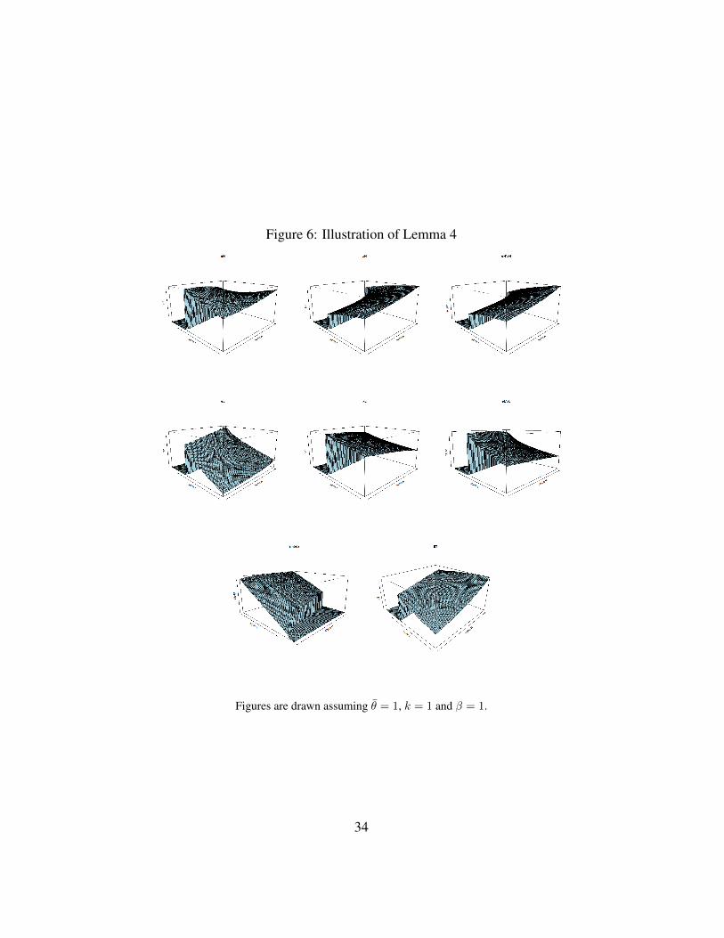
Figure 6: Illustration of Lemma 4
Figures are drawn assuming θ = 1, k = 1 and β = 1.
34

Figure 7: W (αH , αL)
Social welfare pattern when θ = 0.2; 1; 1.8.
35