Mapping patent classifications: portfolio and statisticalanalysis, and the comparison of strengths and weaknesses

Loet Leydesdorff1 • Dieter Franz Kogler2 • Bowen Yan3

Received: 24 February 2017 / Published online: 1 July 2017� The Author(s) 2017. This article is an open access publication

Abstract The Cooperative Patent Classifications (CPC) recently developed cooperatively

by the European and US Patent Offices provide a new basis for mapping patents and

portfolio analysis. CPC replaces International Patent Classifications (IPC) of the World

Intellectual Property Organization. In this study, we update our routines previously based

on IPC for CPC and use the occasion for rethinking various parameter choices. The new

maps are significantly different from the previous ones, although this may not always be

obvious on visual inspection. We provide nested maps online and a routine for generating

portfolio overlays on the maps; a new tool is provided for ‘‘difference maps’’ between

patent portfolios of organizations or firms. This is illustrated by comparing the portfolios of

patents granted to two competing firms—Novartis and MSD—in 2016. Furthermore, the

data is organized for the purpose of statistical analysis.

Keywords Patent � Map � Portfolio � CPC � Diversity � City � Comparisons � SWOT

& Loet Leydesdorffloet@leydesdorff.net

Dieter Franz Koglerdieter.kogler@ucd.ie

Bowen Yanbowen_yan@sutd.edu.sg

1 Amsterdam School of Communication Research (ASCoR), University of Amsterdam,PO Box 15793, 1001 NG Amsterdam, The Netherlands

2 School of Architecture, Planning and Environmental Policy, UCD Centre for Spatial Dynamics,University College Dublin, Richview Campus, Belfield, Dublin 4 D04 V1W8, Ireland

3 SUTD-MIT International Design Centre, Singapore University of Technology and Design,Singapore 487372, Singapore

123

Scientometrics (2017) 112:1573–1591DOI 10.1007/s11192-017-2449-0

Introduction

Patent data provide a primary data source for scholars interested in the development of

technological knowledge (e.g., Strumsky et al. 2012). In a comprehensive study of US

patent data, Jaffe and Trajtenberg (2002), for example, argued that patents and patent

citations provide ‘‘a window on the knowledge economy.’’ However, patents are indicators

of inventions and not innovations (Archibugi and Pianta 1992; Pavitt 1985; Griliches

1990). Like publication data, patent data provide a wealth of information about knowledge

claims (Hunt et al. 2007), references to prior art, forward citation, inventor and applicant

addresses, and classifications. Note that patenting can also be strategic or defensive given a

firm’s technical expertise and product portfolio (Alkemade et al. 2015).

Different from journal articles, patents are not refereed among peers, but by examiners

at the patent office, among other things, on the criterion of whether the submitted appli-

cation provides novelty. The purpose of the novelty requirement is to prevent prior art from

being patented again. The examiner is entitled to add references to prior art,1 but most

importantly organizes the patent in a patent classification system. In the absence of an

equivalent for journals, the classification system can be considered as the intellectual

organization of the database of novel products and processes of economic value.

Jaffe (1986) was the first who proposed to use co-classifications of patents for char-

acterizing the technological positions of firms with the objective of quantifying techno-

logical opportunities and research spillovers. For this purpose, each patent can be

represented as a vector of classifications. Jaffe (1989) used the cosine between these

vectors as a similarity measure (Salton and McGill 1983). Sets of patents (e.g., patent

portfolios of firms) can be modeled as aggregates of these vectors into matrices. The

resulting matrix can be used for statistical analysis and/or the visualization of the simi-

larities as projections on a map (Schiffman et al. 1981; Waltman et al. 2010).

In a series of studies, we developed instruments for the mapping and analysis of patent

data with a focus mainly on data of the US Patent and Trade Office (USPTO). US patenting

is considered the most competitive and is therefore most relevant to technology and

innovation studies (Granstrand 1999; Jaffe 1989; Jaffe and Trajtenberg 2002; Lee 2013).

USPTO maintains a freely available database of patent data at http://patft.uspto.gov/

netahtml/PTO/search-adv.htm. This database is copied at other places, such as Google

Patents, the National Bureau of Economic Research (NBER) in the USA, and PatentsView

(http://www.patentsview.com). PatentsView adds to the data by providing disambiguated

inventor and assignee identifiers (Monath and McCallum 2015).

Building on approaches suggested in previous studies (e.g., Breschi et al. 2003; Leten

et al. 2007; Verspagen 1997), we developed instruments for the mapping and analysis of

patent data using International Patent Classifications (IPC). IPC was developed by the

World International Property Organization (WIPO) and further elaborated by the European

Patent Office (EPO) into the European Classification System ECLA. This classification

uses up to fourteen characters for the indexing. As of 1 January 2013, however, USPTO

and EPO use the new Cooperative Patent Classifications (CPC) which build on ECLA. In

addition to the various patent offices of the EU member states, China, Korea, Russia, and

Mexico, among others, are in the process of aligning their classifications with CPC. In this

study, we use CPC for the mapping, review and integrate the results and routines from the

1 At EPO all references are added by the examiner.

1574 Scientometrics (2017) 112:1573–1591

123

previous studies, revise some of the methodological choices, and update the routines and

analysis accordingly.

Choices of parameters

In addition to the choice of a similarity criterion such as the cosine, a number of parameter

choices are relevant for the mapping of patent data: the choice of domains in terms of

patent offices (USPTO, EPO, WIPO, etc.), the classification system (CPC, IPC, etc.), the

clustering algorithm (e.g., co-classification, co-citation, bibliographic coupling), etc. The

classifications can be used with different levels of detail by using more digits of the

respective classes, i.e. main- and/or sub-classes.

Kogler et al. (2017b) used IPC at the four-digit level for portfolio analysis; Yan and Luo

(2017) used IPC at the three-digit level (IPC-3). Leydesdorff et al. (2014) used both three

and four digits of IPC for exploring a dynamic approach. With similar objectives, Kay

et al. (2014) composed 466 IPC categories at different levels of depth after preprocessing

their data from the comprehensive PATSTAT database.2 Schoen et al. (2012) use a

database of the Corporate Invention Board (CIB) for the construction of their own clas-

sification (Alkemade et al. 2015). Archibugi and Pianta (1992) combined IPC with the

Standard Industrial Classification (SIC) using a concordance table. However, the objective

of these last authors was not to provide a map or overlays.

In this study, we use CPC at the four digit level. CPC is similar to IPC in the first four

digits, but the classification of individual patents can be changed in the process of

reclassification; new classes have also been added. Furthermore, CPC contains new cat-

egories classified under ‘‘Y’’ that span different sections of CPC in order to indicate new

technological developments such as nanotechnology and technologies for the mitigation of

climate change (Scheu et al. 2006; Veefkind et al. 2012). Currently, there are nine of these

Y-classes. Since these boundary-spanning classes are back-tracked into the database, they

introduce new links between previously unrelated classes. As a result, one can expect

changes in the networks among the classes. All values in this study are based on CPC at the

4-digit level (CPC-4) instead of IPC-4.

Co-classification is a binary measure at the level of individual patents. Co-citation of

classes or bibliographic couplings among them can be considered as more refined measures

of the strength of the relationships. Yan and Luo (2017) compared twelve techniques for

the mapping of patent data in terms of citation relations, inventive activities, etc., among

121 IPC classes at the 3-digit level. The conclusion was that maps based on Jaccard-

normalized bibliographic coupling at the (disaggregated) patent level—‘‘A1’’ in the

classification of methods provided by these authors—significantly outperformed maps

based on the cosine values among of aggregated citations among IPC classes (Leydesdorff

et al. 2014, 2015). Actually, Yan and Luo (2017, at p. 435) conclude that ‘‘class-to-class

cosine similarity among aggregated citations (A2) performed the worst in various analyses,

although it is popularly used for constructing network maps of patents.’’ This critique

prompted us to reconsider on previous choices of parameters.

In this study, we combine our two approaches: we use bibliographic coupling among

CPC-4 classes at the level of patents as individual documents. We first construct the

asymmetrical (2-mode) matrix of patents (cited) in the rows versus citing patents

2 Further information regarding access to PATSTAT can be found at: https://www.epo.org/searching-for-patents/business/patstat.html.

Scientometrics (2017) 112:1573–1591 1575

123

aggregated into the 654 CPC classes at the 4-digit level in the columns. The Jaccard index

and cosine values are then computed over the 654 columns (Leydesdorff and Vaughan

2006). The resulting (1-mode) matrices can be utilized as input into the mapping exercise.

For the clustering and subsequent coloring of the resulting map we use a methodology

recently developed by Leydesdorff et al. (2017) for journal mapping. VOSviewer (v1.6.5;

28 September 2016) provides both a community-finding algorithm and visualization

(Waltman et al. 2010). We use this algorithm for generating a hierarchically decomposed

set of maps of patent classes. Although the resulting maps are statistical and cannot claim

semantic authority, they can serve the heuristics by offering a baseline. Both the Jaccard-

based map and the cosine-based one were decomposed into clusters using these statistics.

VOSviewer enables us to visualize 654 data points without cluttering the labels on the

screen by foregrounding and backgrounding strong and weak presences, respectively. The

CPC classes are fractionally counted so that each patent contributes with a value of one.

Methods

Data

We harvested patent data from 1976 to July of 2016 from USPTO and PatentsView3 on

January 11, 2017. The data set contains 5,175,268 utility patents. Each patent is classified

in one or more CPC classes. The definitions of CPC classes are available among other

places at https://www.uspto.gov/web/patents/classification/cpc.html. As noted, CPC and

IPC are identical in terms of the first four digits. However, IPC contains 630 four-digit

classes, whereas CPC distinguishes 705 such classes, of which 654 are currently in use. We

use these 654 classes.

Distance measures

The 5M? patents cite 7,203,533 patents. First, we constructed a 2-mode matrix of the 654

classes—aggregates of the 5M? citing patents—versus the 7M? cited patents. This

matrix was then used for computing the symmetrical 1-mode matrices of 654 * 654 Jac-

card and cosine values, respectively. Equations (1) and (2) provide the formulas for cal-

culating Jaccard and cosine similarity between two random variables.

Jaccard ¼Pn

i¼1 xiyiPni¼1 x

2i þ

Pni¼1 y

2i �

Pni¼1 xiyi

ð1Þ

Cosine ¼Pn

i¼1 xiyiffiffiffiffiffiffiffiffiffiffiffiffiffiffiffiffiPni¼1 x

2i

p ffiffiffiffiffiffiffiffiffiffiffiffiffiffiffiffiPni¼1 y

2i

p ð2Þ

The Jaccard matrix is based on counting the cited patents as binary [A1 in Yan and Luo

(2017)],4 whereas numerical values can be used for computing cosine values: a patent can

be cited more than once in a CPC-class of citing patents. Yan and Luo (2017) categorize

this cosine based on values at the individual patent level as a third option A3 and conclude

3 Patentsview is available at http://www.patentsview.org/.4 A non-binary equivalent of the Jaccard index is provided by the Tanimoto index (Lipkus 1999; cf. Saltonand McGill 1983, at pp. 203f).

1576 Scientometrics (2017) 112:1573–1591

123

that ‘‘in some cases of our analysis, A3 is no worse than A1.’’ However, the QAP (Pearson)

correlation between the resulting two matrices—diagonals excluded—is 0.786

(p\ .0001). Thus, one can also expect the two maps to be different. We explore and

compare both maps.

The cosine can be considered as a proximity measure in the vector space and

(1 - cosine) thus provides a distance measure. While the corresponding ‘‘Jaccard dis-

tance’’ (=1 - Jaccard) is widely accepted in the literature as well, we note that the Jaccard

index in contrast is a relational measure. From the perspective of graph theory, the geo-

desic would be a better measure for the distance between two nodes in a network (de Nooy

et al. 2011). As a distance measure, in our opinion, one should therefore preferably use

(1 - cosine) and not the Jaccard distance.

Clustering

Both the Jaccard and the cosine matrices were decomposed using the routine decomp.exe

(available at http://www.leydesdorff.net/jcr15/program.htm). The maps based on the Jac-

card indices are available (i) at http://www.leydesdorff.net/cpcmaps for each class (bot-

tom-up) and (ii) at http://www.leydesdorff.net/cpcmaps/scope using hierarchical clustering

top-down. One has the option either to access the various maps directly in the.jpg format or

to webstart a map using VOSviewer. The latter option provides an analyst with follow-up

options such as choosing other parameters or exporting the files in formats used by other

software applications.5

Jaccard and cosine values generated on the basis of the 2-mode matrix of patents versus

classes can be very small since these matrices are sparse. During the decomposition, for

example, VOSviewer saves files with fewer decimals than the cosine values so that these

values are rounded to zero. This inflates the modularity and generates small clusters. In

order to avoid this effect, we multiplied all values by 1000. For the global map, this makes

no difference in the case of cosine values and hardly any difference for a map based on

Jaccard values; but the larger values improve the decomposition because the additional

zeros otherwise increase the number of small clusters. However, the larger values can no

longer be used for the distance measurement because they can be larger than one. For this

reason, we use the cosine between aggregated citations among classes as the proximity

measure in the routines about portfolio management. (This file ‘‘cos_cpc.dbf’’ is available at

http://www.leydesdorff.net/cpc_cos/cos_cpc.dbf; see the ‘‘Appendix’’ section for details.)

Portfolios

We provide a routine (CPC.exe; see the ‘‘Appendix’’ section) for generating overlays on

the new map. Overlays on maps can be used for portfolio management by science-policy

makers and R&D management (Kogler et al. 2017b; Leydesdorff et al. 2016; Rotolo et al.

2017). We add to the portfolio mapping, the option of a ‘‘difference map’’ so that one can

visually compare two portfolios in a single map, indicated with two different colors.

5 For the convenience of the user, the symmetrical Jaccard matrix is made available at http://www.leydesdorff.net/cpcmaps/jaccard-sym.csv. Analogously, the cosine-based maps and decompositions arebrought online at http://www.leydesdorff.net/cpc_cos and http://www.leydesdorff.net/cpc_cos/scope,respectively. The symmetrical cosine matrix is available at http://www.leydesdorff.net/cpcmaps/cosine-sym.csv.

Scientometrics (2017) 112:1573–1591 1577

123

Using the routine (made available at http://www.leydesdorff.net/cpc_cos/portfolio/

index.htm; see the ‘‘Appendix’’ section for instructions), one can first retrieve a specific

patent set using any search string valid in the USPTO search interface. The routine then

generates a file vos.txt that can be read by VOSviewer and generate overlays.6 In order to

facilitate comparisons among sets a column variable is added to a file matrix.dbf for each

run. This file can be read into programs such as SPSS for statistical analysis. Similar, a row

variable is added to the file rao.dbf containing the value of Rao-Stirling diversity D (Rao

1982; Stirling 2007) and Zhang et al.’s (2016) improved measure 2D3 [= 1/(1 – D)] for thesample under study. In our opinion, these diversity measures can be considered as mea-

sures of ‘‘related variety’’ (Frenken et al. 2007), since the disparity is measured in addition

to the variety (Rafols and Meyer 2010). The variety is ecologically related in terms of the

disparity among the categories. If the files matrix.dbf and rao.dbf are not already present or

were deleted, they are generated de novo.

The routine CPC.exe first asks for a name of the sample (e.g., ‘‘Boston’’) that is used to

label the column and row variables added. The routine is technically similar to the one

defined in Kogler et al. (2017b) for IPC classes, but based on the improved map using

CPC-4. The routine CPC2.exe asks for two sets of downloaded patents in order to generate

a difference map. Difference maps can be used for comparing portfolios of different units

of analysis.

Results

Jaccard or cosine-based maps?

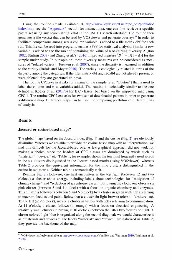
The global maps based on the Jaccard index (Fig. 1) and the cosine (Fig. 2) are obviously

dissimilar. Whereas we are able to provide the cosine-based map with an interpretation, we

find this difficult for the Jaccard-based one. A lexigraphical approach did not work for

making a choice, since the headers of CPC classes are dominated by words such as

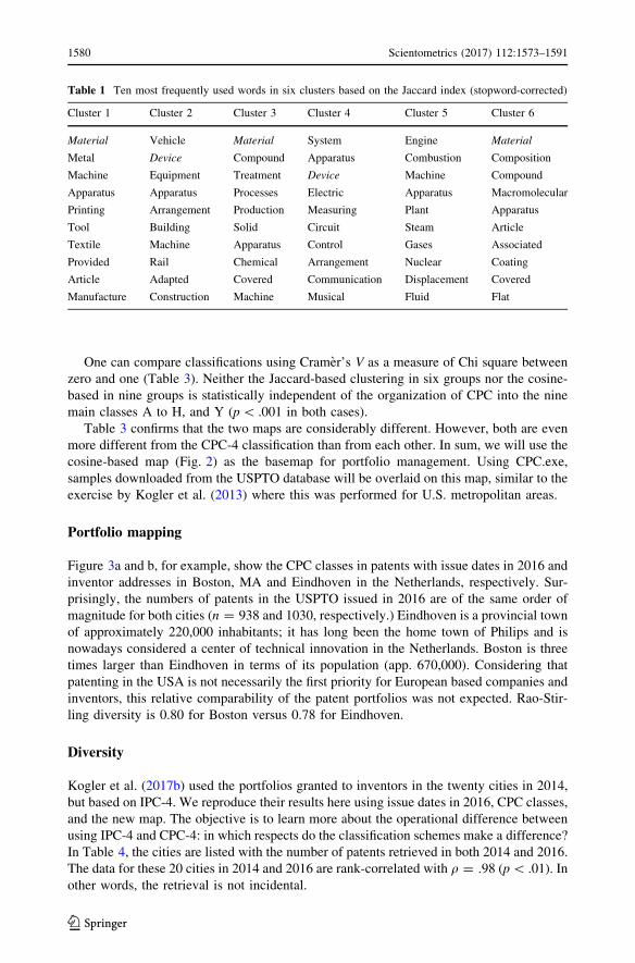
‘‘material,’’ ‘‘device,’’ etc. Table 1, for example, shows the ten most frequently used words

in the six clusters distinguished in the Jaccard-based matrix (using VOSviewer), whereas

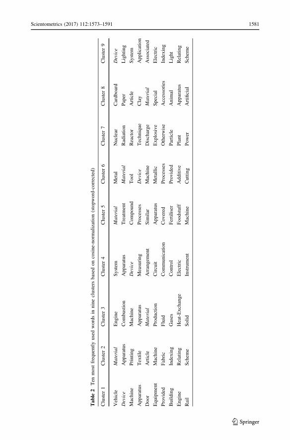
Table 2 provides the equivalent information for the nine clusters distinguished in the

cosine-based matrix. Neither table is semantically rich.

Reading Fig. 2 clockwise, one first encounters at the top right (between 12 and two

o’clock) a cluster about energy, including labels about technologies for ‘‘mitigation of

climate change’’ and ‘‘reduction of greenhouse gases.’’ Following the clock, one observes a

pink cluster (between 3 and 4 o’clock) with a focus on organic chemistry and enzymes.

This cluster is followed (between 5 and 6 o’clock) by a cluster in green with titles referring

to macromolecules and paint. Below that a cluster (in light-brown) refers to furniture, etc.

To the left (at 9 o’clock), we see a cluster in yellow with titles referring to communication.

At 11 o’clock, a cluster follows (in orange) with a focus on electrical engineering. A

relatively small cluster (in brown, at 10 o’clock) between the latter two focuses on light. A

cluster colored light-blue is organized along the second diagonal; we would characterize it

as ‘‘materials and devices.’’ The labels ‘‘material’’ and ‘‘device’’ are italicized in Table 2;

they provide the backbone of the map.

6 VOSviewer is freely available at http://www.vosviewer.com (Van Eck and Waltman 2010; Waltman et al.2010).

1578 Scientometrics (2017) 112:1573–1591

123

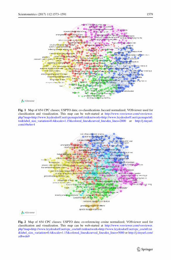
Fig. 1 Map of 654 CPC classes; USPTO data; co-classifications Jaccard normalized; VOSviewer used forclassification and visualization. This map can be web-started at http://www.vosviewer.com/vosviewer.php?map=http://www.leydesdorff.net/cpcmaps/m0.txt&network=http://www.leydesdorff.net/cpcmaps/n0.txt&label_size_variation=0.4&scale=1.15&colored_lines&curved_lines&n_lines=2000 or http://j.tinyurl.com/z9u4nv4

Fig. 2 Map of 654 CPC classes; USPTO data; co-referencing cosine normalized; VOSviewer used forclassification and visualization. This map can be web-started at http://www.vosviewer.com/vosviewer.php?map=http://www.leydesdorff.net/cpc_cos/m0.txt&network=http://www.leydesdorff.net/cpc_cos/n0.txt&label_size_variation=0.4&scale=1.15&colored_lines&curved_lines&n_lines=5000 or http://j.tinyurl.com/zdbwdn9

Scientometrics (2017) 112:1573–1591 1579

123

One can compare classifications using Cramer’s V as a measure of Chi square between

zero and one (Table 3). Neither the Jaccard-based clustering in six groups nor the cosine-

based in nine groups is statistically independent of the organization of CPC into the nine

main classes A to H, and Y (p\ .001 in both cases).

Table 3 confirms that the two maps are considerably different. However, both are even

more different from the CPC-4 classification than from each other. In sum, we will use the

cosine-based map (Fig. 2) as the basemap for portfolio management. Using CPC.exe,

samples downloaded from the USPTO database will be overlaid on this map, similar to the

exercise by Kogler et al. (2013) where this was performed for U.S. metropolitan areas.

Portfolio mapping

Figure 3a and b, for example, show the CPC classes in patents with issue dates in 2016 and

inventor addresses in Boston, MA and Eindhoven in the Netherlands, respectively. Sur-

prisingly, the numbers of patents in the USPTO issued in 2016 are of the same order of

magnitude for both cities (n = 938 and 1030, respectively.) Eindhoven is a provincial town

of approximately 220,000 inhabitants; it has long been the home town of Philips and is

nowadays considered a center of technical innovation in the Netherlands. Boston is three

times larger than Eindhoven in terms of its population (app. 670,000). Considering that

patenting in the USA is not necessarily the first priority for European based companies and

inventors, this relative comparability of the patent portfolios was not expected. Rao-Stir-

ling diversity is 0.80 for Boston versus 0.78 for Eindhoven.

Diversity

Kogler et al. (2017b) used the portfolios granted to inventors in the twenty cities in 2014,

but based on IPC-4. We reproduce their results here using issue dates in 2016, CPC classes,

and the new map. The objective is to learn more about the operational difference between

using IPC-4 and CPC-4: in which respects do the classification schemes make a difference?

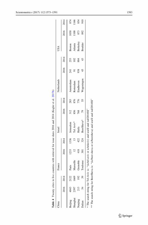
In Table 4, the cities are listed with the number of patents retrieved in both 2014 and 2016.

The data for these 20 cities in 2014 and 2016 are rank-correlated with q = .98 (p\ .01). In

other words, the retrieval is not incidental.

Table 1 Ten most frequently used words in six clusters based on the Jaccard index (stopword-corrected)

Cluster 1 Cluster 2 Cluster 3 Cluster 4 Cluster 5 Cluster 6

Material Vehicle Material System Engine Material

Metal Device Compound Apparatus Combustion Composition

Machine Equipment Treatment Device Machine Compound

Apparatus Apparatus Processes Electric Apparatus Macromolecular

Printing Arrangement Production Measuring Plant Apparatus

Tool Building Solid Circuit Steam Article

Textile Machine Apparatus Control Gases Associated

Provided Rail Chemical Arrangement Nuclear Coating

Article Adapted Covered Communication Displacement Covered

Manufacture Construction Machine Musical Fluid Flat

1580 Scientometrics (2017) 112:1573–1591

123

Table

2Ten

mostfrequentlyusedwordsin

nineclustersbased

oncosine-norm

alization(stopword-corrected)

Cluster

1Cluster

2Cluster

3Cluster

4Cluster

5Cluster

6Cluster

7Cluster

8Cluster

9

Vehicle

Material

Engine

System

Material

Metal

Nuclear

Cardboard

Device

Device

Apparatus

Combustion

Apparatus

Treatment

Material

Radiation

Paper

Lighting

Machine

Printing

Machine

Device

Compound

Tool

Reactor

Article

System

Apparatus

Textile

Apparatus

Measuring

Processes

Device

Technique

Clay

Application

Door

Article

Material

Arrangem

ent

Sim

ilar

Machine

Discharge

Material

Associated

Equipment

Machine

Production

Circuit

Apparatus

Metallic

Explosive

Special

Electric

Provided

Fabric

Fluid

Communication

Covered

Processes

Otherwise

Accessories

Indexing

Building

Indexing

Gases

Control

Fertiliser

Provided

Particle

Anim

alLight

Engine

Relating

Heat-Exchange

Electric

Foodstuff

Additive

Plant

Apparatus

Relating

Rail

Schem

eSolid

Instrument

Machine

Cutting

Power

Artificial

Schem

e

Scientometrics (2017) 112:1573–1591 1581

123

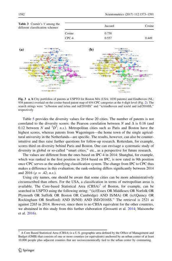
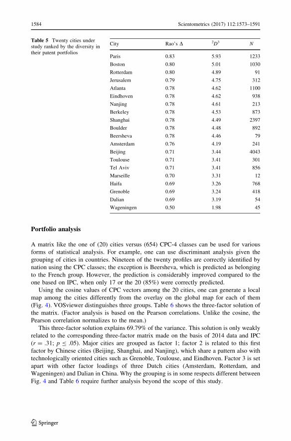
Table 5 provides the diversity values for these 20 cities. The number of patents is not

correlated to the diversity scores: the Pearson correlation between N and D is 0.16 (and

0.12 between N and 2D3; n.s.). Metropolitan cities such as Paris and Boston have the

highest scores, whereas patents from Wageningen—the home town of the single agricul-

tural university in the Netherlands—are specific. The results, however, can also be counter-

intuitive and thus raise further questions for follow-up research. Rotterdam, for example,

scores third on diversity behind Paris and Boston. One can envisage a systematic study of

diversity in global or so-called ‘‘smart cities,’’ etc., as a perspective for future research.

The values are different from the ones based on IPC-4 in 2014: Shanghai, for example,

which was ranked in the first position in 2014 based on IPC, is now rated in 9th position

once CPC serves as the underlying classification system. The change from IPC to CPC thus

makes a difference in this evaluation; the rank-ordering differs significantly between 2014

and 2016 (q = .42; n.s.).

Using city names, one should be aware that some cities can be more administratively

circumscribed than others. For the USA, a classification in terms of metropolitan areas is

available. The Core-based Statistical Area (CBSA)7 of Boston, for example, can be

searched in USPTO using the following string: ‘‘(ic/(Essex OR Middlesex OR Norfolk OR

Plymouth OR Suffolk OR Boston OR Cambridge) AND IS/MA) OR (ic/(Quincy OR

Rockingham OR Strafford) AND IS/NH) AND ISD/2016$$.’’ The retrieval is 2521 as

against 2265 in 2014. However, since there is no CBSA equivalent for the other countries,

we abstained in this study from this further elaboration (Grossetti et al. 2014; Maisonobe

et al. 2016).

Fig. 3 a, b City portfolios of patents at USPTO for Boston MA (USA; 1030 patents) and Eindhoven (NL;938 patents) overlaid on the cosine-based patent map of 654 CPC categories at the 4-digit level (Fig. 2). Thesearch strings were ‘‘ic/boston and is/ma and isd/2016$$’’ and ‘‘ic/eindhoven and icn/nl and isd/2016$$,’’respectively

Table 3 Cramer’s V among thedifferent classification schemes

Jaccard Cosine

Cosine 0.758

CPC-4 0.557 0.449

7 A Core Based Statistical Area (CBSA) is a U.S. geographic area defined by the Office of Management andBudget (OMB) that consists of one or more counties (or equivalents) anchored by an urban center of at least10,000 people plus adjacent counties that are socioeconomically tied to the urban center by commuting.

1582 Scientometrics (2017) 112:1573–1591

123

Table

4Twenty

cities

infivecountrieswithretrieval

forissuedates

2016and2014(K

ogleret

al.2017b)

China

France

Israel

Netherlands

USA

2016

2014

2016

2014

2016

2014

2016

2014

2016

2014

Beijing

4043

2122

Paris

1233

1336

Jerusalem

312

283

Amsterdam

241

253

Boston

1030

874

Shanghai

2397

1669

Marseille

12

13

Tel

Aviv*

856

876

Rotterdam

91

102

Atlanta

1100

1166

Nanjing

213

192

Grenoble

418

422

Haifa

768

776

Eindhoven

938

884

Berkeley

873

854

Dalian

54

39

Toulouse

301

324

BeerSheva*

79

55

Wageningen

45

43

Boulder

892

910

*Thesearch

stringforTel-A

viv

is:‘‘(ic/tel-aviv

oric/telaviv)andicn/ilandisd/2014$$’’

**Thesearch

stringforBeerShevais:‘‘(ic/beer-shevaoric/beersheva)

andicn/ilandisd/2014$$’’

Scientometrics (2017) 112:1573–1591 1583

123

Portfolio analysis

A matrix like the one of (20) cities versus (654) CPC-4 classes can be used for various

forms of statistical analysis. For example, one can use discriminant analysis given the

grouping of cities in countries. Nineteen of the twenty profiles are correctly identified by

nation using the CPC classes; the exception is Beersheva, which is predicted as belonging

to the French group. However, the prediction is considerably improved compared to the

one based on IPC, when only 17 or the 20 (85%) were correctly predicted.

Using the cosine values of CPC vectors among the 20 cities, one can generate a local

map among the cities differently from the overlay on the global map for each of them

(Fig. 4). VOSviewer distinguishes three groups. Table 6 shows the three-factor solution of

the matrix. (Factor analysis is based on the Pearson correlations. Unlike the cosine, the

Pearson correlation normalizes to the mean.)

This three-factor solution explains 69.79% of the variance. This solution is only weakly

related to the corresponding three-factor matrix made on the basis of 2014 data and IPC

(r = .31; p B .05). Major cities are grouped as factor 1; factor 2 is related to this first

factor by Chinese cities (Beijing, Shanghai, and Nanjing), which share a pattern also with

technologically oriented cities such as Grenoble, Toulouse, and Eindhoven. Factor 3 is set

apart with other factor loadings of three Dutch cities (Amsterdam, Rotterdam, and

Wageningen) and Dalian in China. Why the grouping is in some respects different between

Fig. 4 and Table 6 require further analysis beyond the scope of this study.

Table 5 Twenty cities understudy ranked by the diversity intheir patent portfolios

City Rao’s D 2D3 N

Paris 0.83 5.93 1233

Boston 0.80 5.01 1030

Rotterdam 0.80 4.89 91

Jerusalem 0.79 4.75 312

Atlanta 0.78 4.62 1100

Eindhoven 0.78 4.62 938

Nanjing 0.78 4.61 213

Berkeley 0.78 4.53 873

Shanghai 0.78 4.49 2397

Boulder 0.78 4.48 892

Beersheva 0.78 4.46 79

Amsterdam 0.76 4.19 241

Beijing 0.71 3.44 4043

Toulouse 0.71 3.41 301

Tel Aviv 0.71 3.41 856

Marseille 0.70 3.31 12

Haifa 0.69 3.26 768

Grenoble 0.69 3.24 418

Dalian 0.69 3.19 54

Wageningen 0.50 1.98 45

1584 Scientometrics (2017) 112:1573–1591

123

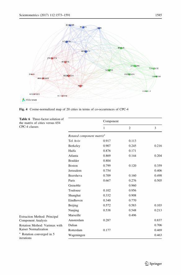
Fig. 4 Cosine-normalized map of 20 cities in terms of co-occurrences of CPC-4

Table 6 Three-factor solution ofthe matrix of cities versus 654CPC-4 classes

Extraction Method: PrincipalComponent Analysis

Rotation Method: Varimax withKaiser Normalizationa Rotation converged in 5iterations

Component

1 2 3

Rotated component matrixa

Tel Aviv 0.917 0.113

Berkeley 0.907 0.245 0.216

Haifa 0.876 0.171

Atlanta 0.869 0.144 0.204

Boulder 0.804

Boston 0.799 0.120 0.359

Jerusalem 0.754 0.406

Beersheva 0.709 0.160 0.498

Paris 0.667 0.276 0.505

Grenoble 0.960

Toulouse 0.102 0.956

Shanghai 0.332 0.908

Eindhoven 0.340 0.770

Beijing 0.572 0.583 0.103

Nanjing 0.538 0.548 0.213

Marseille 0.496

Amsterdam 0.287 0.837

Dalian 0.706

Rotterdam 0.177 0.469

Wageningen 0.463

Scientometrics (2017) 112:1573–1591 1585

123

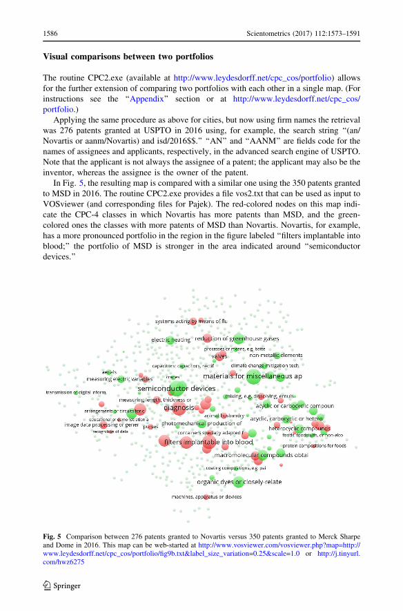
Visual comparisons between two portfolios

The routine CPC2.exe (available at http://www.leydesdorff.net/cpc_cos/portfolio) allows

for the further extension of comparing two portfolios with each other in a single map. (For

instructions see the ‘‘Appendix’’ section or at http://www.leydesdorff.net/cpc_cos/

portfolio.)

Applying the same procedure as above for cities, but now using firm names the retrieval

was 276 patents granted at USPTO in 2016 using, for example, the search string ‘‘(an/

Novartis or aanm/Novartis) and isd/2016$$.’’ ‘‘AN’’ and ‘‘AANM’’ are fields code for the

names of assignees and applicants, respectively, in the advanced search engine of USPTO.

Note that the applicant is not always the assignee of a patent; the applicant may also be the

inventor, whereas the assignee is the owner of the patent.

In Fig. 5, the resulting map is compared with a similar one using the 350 patents granted

to MSD in 2016. The routine CPC2.exe provides a file vos2.txt that can be used as input to

VOSviewer (and corresponding files for Pajek). The red-colored nodes on this map indi-

cate the CPC-4 classes in which Novartis has more patents than MSD, and the green-

colored ones the classes with more patents of MSD than Novartis. Novartis, for example,

has a more pronounced portfolio in the region in the figure labeled ‘‘filters implantable into

blood;’’ the portfolio of MSD is stronger in the area indicated around ‘‘semiconductor

devices.’’

Fig. 5 Comparison between 276 patents granted to Novartis versus 350 patents granted to Merck Sharpeand Dome in 2016. This map can be web-started at http://www.vosviewer.com/vosviewer.php?map=http://www.leydesdorff.net/cpc_cos/portfolio/fig9b.txt&label_size_variation=0.25&scale=1.0 or http://j.tinyurl.com/hwz6275

1586 Scientometrics (2017) 112:1573–1591

123

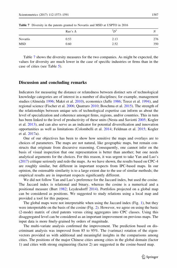
Table 7 shows the diversity measures for the two companies. As might be expected, the

values for diversity are much lower in the case of specific industries or firms than in the

case of cities (see Table 5).

Discussion and concluding remarks

Indicators for measuring the distance or relatedness between distinct sets of technological

knowledge categories are of interest in a number of disciplines; for example, management

studies (Almeida 1996; Makri et al. 2010), economics (Jaffe 1986; Teece et al. 1994), and

regional science (Fischer et al. 2006; Quatraro 2010; Boschma et al. 2015). The strength of

the relationships between unique sets of technological expertise can inform us about the

level of specialization and coherence amongst firms, regions, and/or countries. This in turn

has been linked to the level of productivity of these units (Nesta and Saviotti 2005; Kogler

et al. 2013), and can also serve as an indicator for potential diversification and innovation

opportunities as well as limitations (Colombelli et al. 2014; Feldman et al. 2015; Kogler

et al. 2017a).

One of our objectives has been to show how sensitive the maps and overlays are to

choices of parameters. The maps are not natural, like geographic maps, but remain con-

structs that originate from discursive reasoning. Consequently, one cannot infer on the

basis of visual inspection that one representation is better than another; but one needs

analytical arguments for the choices. For this reason, it was urgent to take Yan and Luo’s

(2017) critique seriously and redo the maps. As we have shown, the results based on CPC-4

are roughly similar, but different in important respects from IPC-based maps. In our

opinion, the ostensable similarity is to a large extent due to the use of similar methods; the

empirical results are in important respects significantly different.

We did not follow Yan and Luo’s preference for the Jaccard index, but used the cosine.

The Jaccard index is relational and binary, whereas the cosine is a numerical and a

positional measure (Burt 1982; Leydesdorff 2014). Portfolios projected on a global map

can be considered as positions. We suggested to study relations using a local map and

provided a tool for this purpose.

The global maps were not interpretable when using the Jaccard index (Fig. 1), but they

were interpretable on the basis of the cosine (Fig. 2). However, we agree on using the basic

(2-mode) matrix of cited patents versus citing aggregates into CPC classes. Using this

disaggregated level can be considered as an important improvement on previous maps. The

input data is more finely-grained by orders of magnitude.

The multi-variate analysis confirmed the improvement. The prediction based on dis-

criminant analysis was improved from 85 to 95%. The (varimax) rotation of the eigen-

vectors provided us with additional and meaningful insights in the comparisons among

cities. The positions of the major Chinese cities among cities in the global domain (factor

1) and cities with strong engineering (factor 2) are suggested in the cosine-based map.

Table 7 Diversity in the patents granted to Novartis and MSD at USPTO in 2016

Rao’s D 2D3 N

Novartis 0.53 2.13 276

MSD 0.60 2.52 350

Scientometrics (2017) 112:1573–1591 1587

123

Visualization is a strong instrument because maps can be provided with an interpre-

tation more easily than numerical statistics. However, the latter are needed in the back-

ground for making analytical arguments. A direct comparison between two units (e.g.,

competing firms) using a map, however, can provide a first orientation to their differences

in terms of strengths and weaknesses.

Acknowledgements We are grateful to Jordan Comins and two anonymous referees for comments on aprevious draft. BY acknowledges support by the Academic Research Fund Tier 2 of the Singapore Ministryof Education. DK acknowledges funding by the European Research Council, Grant no. 715631.

Open Access This article is distributed under the terms of the Creative Commons Attribution 4.0 Inter-national License (http://creativecommons.org/licenses/by/4.0/), which permits unrestricted use, distribution,and reproduction in any medium, provided you give appropriate credit to the original author(s) and thesource, provide a link to the Creative Commons license, and indicate if changes were made.

Appendix

1. Preparing input files

(a) Download the following files from http://www.leydesdorff.net/cpc_cos/

portfolio (or https://leydesdorff.github.io/cpc/portfolio) into a single folder on

your hard disk:

• cpc.exe;

• cpc.dbf (with basic information about the classes);

• uspto1.exe (needed for the downloading of USPTO patents);

• cos_cpc.dbf (needed for the computation of distances on the map);

(b) Run cpc.exe

2. Options within cpc.exe

(a) The program asks for a short name (B10 characters) in each run. This name will

be used as the variable label in later parts of the routine;

(b) The first option is to download the patents from USPTO at http://patft.uspto.

gov/netahtml/PTO/search-adv.htm; detailed instructions for the downloading

can be found at http://www.leydesdorff.net/ipcmaps;

(c) USPTO has a maximum of 1000 records at a time, but one is allowed to follow-

up batches; after the download is completed, save the files in another folder or

as a zip file;

3. The incremental construction of the files matrix.dbf and rao.dbf

(a) After each run, a column variable is added to the (local) file matrix.dbf

containing the distribution of the 654 CPC classes in the document set under

study. If the file matrix.dbf is absent, it is generated de novo and the current run

is considered as generating the first variable; matrix.dbf can be read by Excel,

SPSS, etc., for further (statistical) analysis;

1588 Scientometrics (2017) 112:1573–1591

123

(b) Similarly, a row variable is added after each run to the file rao.dbf containing

diversity measures (explained in the article) as variables. This file is also

generated de novo if previously absent. Distances are based on [1 - cos(x,y)]

for each two distributions x and y of aggregated citation at the level of CPC-4

classes;

(c) The routine cpc2cos.exe reads the file matrix.dbf and produces cosine.net and

coocc.dat as (normalized) co-occurrence matrices that can be used in network

analysis and visualization programs such as Pajek or UCInet.

4. Output files in each run

(a) The file ‘‘vos.txt’’ can be read by VOSviewer for mapping the portfolio under

study at the four-digit level of CPC; the distances and colors (corresponding to

clusters) in the maps are based on the base-map provided in Fig. 2 above;

(b) The files cpc.vec and cpc.cls can be used as a vector and cluster files in the

Pajek file provided at http://www.leydesdorff.net/cpc_cos/. This allows for

layouts other than VOSviewer and for more detailed network analysis and

statistics. The file cpc.cls is a so-called cluster file which can be used in Pajek,

among other things, for the extraction of partitions.

(c) The various fields in the USPTO records are organized in a series of databases

that can be related (e.g., in MS Access) using the field ‘‘nr.’’

5. Visual comparison among portfolios (using cpc2.exe)

One can compare two portfolios (as in Fig. 5 above) using cpc2.exe (available at

http://www.leydesdorff.net/cpc_cos/portfolio/cpc2.exe).

(a) One first runs cpc.exe for the one set (e.g., city1);

(b) Replace the downloaded patents (p1.htm, p2.htm, etc.) with the set for the

second unit (e.g., city2) and run cpc2.exe;

(c) The file vos2.txt generated is an input file to VOSviewer. The red-colored nodes

indicate the CPC-4 classes in which the first unit is stronger than the second; the

green-colored nodes indicate the relative strength of the second set;

(d) The files cpc2.vec and cpc2.cls provide the corresponding input files for Pajek.

References

Alkemade, F., Heimeriks, G., Schoen, A., Villard, L., & Laurens, P. (2015). Tracking the international-ization of multinational corporate inventive activity: National and sectoral characteristics. ResearchPolicy, 44(9), 1763–1772.

Almeida, P. (1996). Knowledge sourcing by foreign multinationals: Patent citation analysis in the U.S.semiconductor industry. Strategic Management Journal, 17, 155–165.

Archibugi, D., & Pianta, M. (1992). Specialization and size of technological activities in industrial coun-tries: The analysis of patent data. Research Policy, 21(1), 79–93.

Boschma, R., Balland, P.-A., & Kogler, D. F. (2015). Relatedness and technological change in cities: Therise and fall of technological knowledge in U.S. metropolitan areas from 1981 to 2010. Industrial andCorporate Change, 24, 223–250.

Breschi, S., Lissoni, F., & Malerba, F. (2003). Knowledge-relatedness in firm technological diversification.Research Policy, 32(1), 69–87.

Burt, R. S. (1982). Toward a structural theory of action. New York: Academic Press.

Scientometrics (2017) 112:1573–1591 1589

123

Colombelli, A., Krafft, J., & Quatraro, F. (2014). The emergence of new technology-based sectors inEuropean regions: A proximity-based analysis of nanotechnology. Research Policy, 43(10),1681–1696.

de Nooy, W., Mrvar, A., & Batgelj, V. (2011). Exploratory social network analysis with Pajek (2nd ed.).New York, NY: Cambridge University Press.

Feldman, M. P., Kogler, D. F., & Rigby, D. L. (2015). rKnowledge: The spatial diffusion and adoption ofrDNA methods. Regional Studies, 49(5), 798–817.

Fischer, M., Scherngell, T., & Jansenberger, E. (2006). The geography of knowledge spillovers betweenhigh-technology firms in Europe: Evidence from a spatial interaction modeling perspective. Geo-graphical Analysis, 38, 288–309.

Frenken, K., Van Oort, F., & Verburg, T. (2007). Related variety, unrelated variety and regional economicgrowth. Regional Studies, 41(5), 685–697.

Granstrand, O. (1999). The economics and management of intellectual property: Towards intellectualcapitalism. Cheltenham: Edward Elgar.

Griliches, Z. (1990). Patent statistics as economic indicators: A survey. Journal of Economic Literature, 28,1661–1707.

Grossetti, M., Eckert, D., Gingras, Y., Jegou, L., Lariviere, V., & Milard, B. (2014). Cities and the geo-graphical deconcentration of scientific activity: A multilevel analysis of publications (1987–2007).Urban Studies, 51(10), 2219–2234.

Hunt, D., Nguyen, L., & Rodgers, M. (Eds.). (2007). Patent searching. Hoboken, NJ: Wiley.Jaffe, A. (1986). Technological opportunity and spillovers of R&D. American Economic Review, 76,

984–1001.Jaffe, A. B. (1989). Characterizing the ‘‘technological position’’ of firms, with application to quantifying

technological opportunity and research spillovers. Research Policy, 18(2), 87–97.Jaffe, A. B., & Trajtenberg, M. (2002). Patents, citations, and innovations: A window on the knowledge

economy. Cambridge, MA: MIT Press.Kay, L., Newman, N., Youtie, J., Porter, A. L., & Rafols, I. (2014). Patent overlay mapping: Visualizing

technological distance. Journal of the Association for Information Science and Technology, 65(12),2432–2443.

Kogler, D. F., Essletzbichler, J., & Rigby, D. L. (2017a). The evolution of specialization in the EU15knowledge space. Journal of Economic Geography, 17(2), 345–373.

Kogler, D. F., Heimeriks, G., & Leydesdorff, L. (2017b). Patent portfolio analysis of cities: Statistics andmaps of technological inventiveness. arXiv preprint arXiv:1612.05810. (under submission).

Kogler, D. F., Rigby, D. L., & Tucker, I. (2013). Mapping knowledge space and technological relatedness inUS cities. European Planning Studies, 21, 1374–1391.

Lee, K. (2013). Schumpeterian analysis of economic catch-up: Knowledge, path-creation, and the middle-income trap. Cambridge: Cambridge University Press.

Leten, B., Belderbros, R., & Van Looy, B. (2007). Technological diversification, coherence, and perfor-mance of firms. Journal of Product Innovation and Management, 24, 567–579.

Leydesdorff, L. (2014). Science visualization and discursive knowledge. In B. Cronin & C. Sugimoto (Eds.),Beyond bibliometrics: Harnessing multidimensional indicators of scholarly impact (pp. 167–185).Cambridge, MA: MIT Press.

Leydesdorff, L., Alkemade, F., Heimeriks, G., & Hoekstra, R. (2015). Patents as instruments for exploringinnovation dynamics: Geographic and technological perspectives on ‘‘photovoltaic cells.’’ Sciento-metrics, 102(1), 629–651. doi:10.1007/s11192-014-1447-8.

Leydesdorff, L., Bornmann, L., & Wagner, C. S. (2017). Generating clustered journal maps: An automatedsystem for hierarchical classification. Scientometrics, 110(3), 1601–1614. doi:10.1007/s11192-016-2226-5.

Leydesdorff, L., Heimeriks, G., & Rotolo, D. (2016). Journal portfolio analysis for countries, cities, andorganizations: Maps and comparisons. Journal of the Association for Information Science and Tech-nology, 76(3), 741–748. doi:10.1002/asi.23551.

Leydesdorff, L., Kushnir, D., & Rafols, I. (2014). Interactive overlay maps for US patent (USPTO) databased on international patent classifications (IPC). Scientometrics, 98(3), 1583–1599. doi:10.1007/s11192-012-0923-2.

Leydesdorff, L., & Vaughan, L. (2006). Co-occurrence matrices and their applications in informationscience: Extending ACA to the web environment. Journal of the American Society for InformationScience and Technology, 57(12), 1616–1628.

Lipkus, A. H. (1999). A proof of the triangle inequality for the Tanimoto distance. Journal of MathematicalChemistry, 26(1), 263–265.

1590 Scientometrics (2017) 112:1573–1591

123

Maisonobe, M., Eckert, D., Grossetti, M., Jegou, L., & Milard, B. (2016). The world network of scientificcollaborations between cities: Domestic or international dynamics? Journal of Informetrics, 10(4),1025–1036.

Makri, M., Hitt, M. A., & Lane, P. J. (2010). Complementary technologies, knowledge relatedness, andinvention outcomes in high technology mergers and acquisitions. Strategic Management Journal, 31,602–628.

Monath, N., & McCallum, A. (2015). Discriminative hierarchical coreference for inventor disambiguation.Presented at the PatentsView Inventor Disambiguation Technical Workshop, USPTO, Alexandria, VA,2015.

Nesta, L., & Saviotti, P. P. (2005). Coherence of the knowledge base and the firm’s innovative performance:Evidence from the U.S. pharmaceutical industry. Journal of Industrial Economics, 53(1), 123–142.

Pavitt, K. (1985). Patent statistics as indicators of innovative activities: Possibilities and problems. Scien-tometrics, 7, 77–99.

Quatraro, F. (2010). Knowledge coherence, variety and economic growth: Manufacturing evidence fromItalian regions. Research Policy, 39, 1289–1302.

Rafols, I., & Meyer, M. (2010). Diversity and network coherence as indicators of interdisciplinarity: Casestudies in bionanoscience. Scientometrics, 82(2), 263–287.

Rao, C. R. (1982). Diversity: Its measurement, decomposition, apportionment and analysis. Sankhya: TheIndian Journal of Statistics, Series A, 44(1), 1–22.

Rotolo, D., Rafols, I., Hopkins, M. M., & Leydesdorff, L. (2017). Strategic intelligence on emergingtechnologies: Scientometric overlay mapping. Journal of the Association for Information Science andTechnology, 68(1), 214–233. doi:10.1002/asi.23631.

Salton, G., & McGill, M. J. (1983). Introduction to modern information retrieval. Auckland: McGraw-Hill.Scheu, M., Veefkind, V., Verbandt, Y., Galan, E. M., Absalom, R., & Forster, W. (2006). Mapping

nanotechnology patents: The EPO approach. World Patent Information, 28, 204–211.Schiffman, S. S., Reynolds, M. L., & Young, F. W. (1981). Introduction to multidimensional scaling:

Theory, methods, and applications. New York: Academic Press.Schoen, A., Villard, L., Laurens, P., Cointet, J.-P., Heimeriks, G., & Alkemade, F. (2012). The network

structure of technological developments; Technological distance as a walk on the technology map.Paper presented at the Science & Technology Indicators (STI) Conference 2012 Montreal.

Stirling, A. (2007). A general framework for analysing diversity in science, technology and society. Journalof the Royal Society, Interface, 4(15), 707–719.

Strumsky, D., Lobo, J., & Van der Leeuw, S. (2012). Using patent technology codes to study technologicalchange. Economics of Innovation and New Technology, 21, 267–286.

Teece, D., Rumelt, R., Dosi, G., & Winter, S. (1994). Understanding corporate coherence: Theory andevidence. Journal of Economic Behavior & Organization, 23, 1–30.

Van Eck, N. J., & Waltman, L. (2010). Software survey: VOSviewer, a computer program for bibliometricmapping. Scientometrics, 84(2), 523–538.

Veefkind, V., Hurtado-Albir, J., Angelucci, S., Karachalios, K., & Thumm, N. (2012). A new EPO clas-sification scheme for climate change mitigation technologies. World Patent Information, 34(2),106–111.

Verspagen, B. (1997). Measuring intersectoral technology spillovers: Estimates from the European and USPatent Office Databases. Economic Systems Research, 9, 47–65.

Waltman, L., van Eck, N. J., & Noyons, E. (2010). A unified approach to mapping and clustering ofbibliometric networks. Journal of Informetrics, 4(4), 629–635.

Yan, B., & Luo, J. (2017). Measuring technological distance for patent mapping. Journal of the Associationfor Information Science and Technology, 68(2), 423–437.

Zhang, L., Rousseau, R., & Glanzel, W. (2016). Diversity of references as an indicator for interdisciplinarityof journals: Taking similarity between subject fields into account. Journal of the American Society forInformation Science and Technology, 67(5), 1257–1265. doi:10.1002/asi.23487.

Scientometrics (2017) 112:1573–1591 1591

123