Msa

Fa

b

a

ARRA

KLSSSM

1

sfidsphail2

(G

h1

Ecological Indicators 46 (2014) 367–378

Contents lists available at ScienceDirect

Ecological Indicators

j o ur na l ho me page: www.elsev ier .com/ locate /eco l ind

apping landscape services, spatial synergies and trade-offs. A casetudy using variogram models and geostatistical simulations in angrarian landscape in North-East Germany

abrizio Ungaroa,b,∗, Ingo Zasadaa, Annette Piorra

Leibniz Centre for Agricultural Landscape Research (ZALF), Institute of Socio-Economics, Eberswalder Str. 84, 15374 Müncheberg, GermanyNational Research Council, Institute for Biometeorology (CNR Ibimet), Via Madonna del Piano 10, 50019 Sesto Fiorentino, Italy

r t i c l e i n f o

rticle history:eceived 20 December 2013eceived in revised form 23 June 2014ccepted 27 June 2014

eywords:andscape servicespatial heterogeneityemivariogramsequential simulationsultiple service hotspots

a b s t r a c t

This paper presents a probabilistic approach for mapping and assessment of services provided by land-scapes, based on variogram modelling and geostatistical simulations. Of operational value is that severalservices can be treated and mapped simultaneously, providing an efficient tool to model the heterogene-ity of different landscape components. The methodology was adopted to depict spatial heterogeneity offive landscape services in the case study area of Märkische Schweiz in North East Germany: habitat forspecies, crop production, visual appreciation, water supply, and water regulation. Results, displayed interms of single and joint probability maps, provide new insights about the composition and interrelationof multiple services in a region. It is shown that each landscape service is characterised by a specificspatial pattern, described in terms of heterogeneity and spatial range. Setting a probability threshold ofservice occurrence >0.50, 10% of the area under agricultural land uses provides no landscape services,35% delivers one service while 25% and 19% supply two and three services, respectively. The share of agri-

cultural area with a potential joint provision of four services equals 10%, while only 1.4% of the area hasa potential to deliver five joint landscape services. The highest mean join probability is that observed forthe common supply of production and habitat services (30%), highlighting the occurrence of hotspots ofservices provision with possible conflicts due to the on-going intensification of agricultural management.

. Introduction

Among the growing stock of research in ecosystem and land-cape functions and services (de Groot et al., 2010; TEEB, 2010),actors determining their main spatial characteristics, i.e. variabil-ty and extent, are often overlooked. Their consideration requiresevelopment of methods and tools to quantify and map differentervices across the landscape (Anton et al., 2010). In order to sup-ort sustainable land use decision-making, the analysis of spatialeterogeneity and patterns of the diverse functions and servicescross a given landscape should be able to explore and identify

nteraction effects and potential spatial synergies, i.e. ‘multiple winocations’ or multifunctional ‘hotspots’ (Gimona and van der Horst,007; Egoh et al., 2008; Wu et al., 2013). The availability of spatially

∗ Corresponding author at: Leibniz-Centre for Agricultural Landscape ResearchZALF e.V.), Institute of Socio-Economics, Eberswalder Str. 84, 15374 Muencheberg,ermany. Tel.: +49 33432 82 235; fax: +49 33432 82 308.

E-mail addresses: fabrizio.ungaro@zalf.de, f.ungaro@ibimet.cnr.it (F. Ungaro).

ttp://dx.doi.org/10.1016/j.ecolind.2014.06.039470-160X/© 2014 Elsevier Ltd. All rights reserved.

© 2014 Elsevier Ltd. All rights reserved.

explicit information on the state and trends of these functions andservices is crucial to support valuation and to inform landscapepolicies and decision making (Maes et al., 2012; Syrbe and Walz,2012).

Although the terms landscape and ecosystem services areoften used as synonymous (Lamarque et al., 2011), we preferto use the former over the latter as processes-pattern relation-ships are more clearly understood and modelled at landscape scale(Termorshuizen and Opdam, 2009; van Zanten et al., 2013). Fur-thermore recent studies point out that local stakeholders have abetter understanding of the broader concept of “landscape” than“ecosystem” (Fagerholm et al., 2012; Gulickx et al., 2013), as thelandscape can be viewed as the spatial context where natural andsocio-economic systems intersect (Wu et al., 2013).

There is a growing body of available literature on land-scape service mapping which highlights a number of different

methodological approaches at different spatial and temporal scales(Baral et al., 2013), including land use/cover based assessments(Burkhard et al., 2012; Haines-Young et al., 2012; Koschke et al.,2012), bio-physically based modelling (Bryan and Crossman, 2013),

3 l Indic

ltoBst(ar2cBmltqhocmi

sa1sthvr21a(saett

2

2

StTogcp1l(LG1(7labas

68 F. Ungaro et al. / Ecologica

andscape-landform type mapping (Hermann et al., 2014), ecosys-em structure mapping (Lavorel et al., 2011; Brown et al., 2013)r dynamic process-based ecosystem models (Kareiva et al., 2011;agstad et al., 2013). As effective spatial scales and patterns of land-cape services vary, scale dependency must be taken into accounto select the proper approach depending of the indicators to mapGulickx et al., 2013). Some of the existing modelling approachesre more suitable for large scale studies, where services are directlyelated to land use and are typically qualitative (e.g. Burkhard et al.,012), while others, such as those based upon modelling outputs,an have application from the plot to the landscape scale (e.g.ryan and Crossman, 2013). Yet, the application of spatially explicitethods that incorporate the locations of supply and demand of

andscape services represents a key challenge for research, andhere is the necessity to develop and test different approaches touantify and (jointly) map different services across the landscape,ighlighting “hotspots” with synergies and conflicts. Therefore thebjective of this study is to present a flexible and generally appli-able probabilistic approach to landscape scale assessment andapping of different landscape services. We apply the approach

n the case study area Märkische Schweiz in North-East Germany.Within this framework, highly adaptable and consistent, land-

cape elements and services are considered as the realisation of stochastic process called random function (Chilès and Delfiner,999). Their spatial properties can be described and modelled usingecond order statistics, such as the variogram which describeshe spatial relationships between data and models the spatialeterogeneity of the different landscape components. The use ofariograms and other geostatistical tools to model and map envi-onmental variables is not new in environmetrics (Jensen et al.,006) and landscape ecology (Rossi et al., 1992; Maisel and Turner,998), and an applications to linear landscape elements mappingt small scale has been recently provided by van der Zanden et al.2013). Nevertheless, their potential in landscape services provi-ion assessment has not yet been fully tested and assessed. To thisim, objectives of this work are to analyse and model the spatial het-rogeneity and patterns of the diverse functions and services acrosshe given landscape, and to explore and identify in probabilisticerms services hotspots and ranges.

. Material and methods

.1. Study area

The case study area (576.4 km2) is located in the Federaltate of Brandenburg, extending from the Eastern fringe of Berlinowards the Odra valley at the German-Polish border (Fig. 1a).he landscape morphology was shaped by cyclic glacial advancesf terrestrial Scandinavian ice sheets as well as by peri-glacialeomorphologic processes, resulting in heterogeneous naturalonditions in terms of geomorphology, pedology and topogra-hy (Scholz, 1962), with elevation ranging between 5.8 m and44 m a.m.s.l. Based on geomorphology, dominant soils and related

and cover, the area is subdivided into six major sub-landscapesMeynen and Schmithüsen, 1962, Fig. 1b): Glacial valleys: (i) Rotesuch (45.0 km2, 7.8%) and (ii) Buckow Valley (92.0 km2, 15.6%);round- and end-moraines plateaux: (iii) Lebus Plateau (88.1 km2,5.3%), (iv) Barnim Plateau (206.6 km2, 37.8%) and (v) Oberbarnim88.0 km2, 15.3%); Slope sides; (vi) River Oder Valley (45.0 km2,.8%). The soil typologies, with the exceptions in the River Oder Val-

ey and some areas in the ground and loamy terminal moraines, are

ll characterised by a general low fertility (Fig. 1c). This is assessedased on the German Soil Evaluation System as being between 30nd 60 for arable land and between 30 and 50 for grassland in acale from 0 to 100 (MLUR, 2000).

ators 46 (2014) 367–378

Forest areas (39.9% of total area) cover the largest proportionof the plateau and moraines areas (49.0%), while agricultural lands(45.8% of the total area) are dominant in the ground and loamy ter-minal moraines, representing nearly 73% of these areas (EEA, 2007,Fig. 1a). Due to the disadvantaged natural conditions, nearly all thearea (94%) is subject to the less-favoured area scheme (LFA, CouncilRegulation (EC) No 1698/2005). Additionally, nearly half of the areais designated for nature conservation with NATURA 2000 (Direc-tive 92/43/EEC) and Flora–Fauna–Habitat (Directive 92/43/EEC)areas covering 31% and 9%, respectively, of agricultural land. Intotal, about 43% of the territory (245 km2) is designated for natureconservation of various status. The major protection area is theNaturpark Märkische Schweiz (205 km2). Due to its mixture of for-est and farmland patches, the case study area appears as half-opencountryside with the potential to provide various landscape ser-vices, including food and fibre production natural amenities, waterresource provision, species habitat and recreation.

2.2. Landscape structures and services

Landscape services are defined as “the goods and services pro-vided by landscape to satisfy human needs, directly or indirectly”(Termorshuizen and Opdam, 2009). Examples of landscape servicesare food production, pollination, water regulation, and provisionof recreation (Gulickx et al., 2013). Valuation of landscape andecosystem services through stakeholders has been applied in manystudies (Hein et al., 2006). Therefore, landscape services subject tothis study have been identified and selected by relevance for theregion. In January 2013, 13 local stakeholders from administration,regional management, NGOs and agriculture carried out a priori-tisation and weighting procedure of landscape services based oninter-linkages with land management on the one side and with theendowment for regional socio-economic welfare and competitive-ness on the other. As result, habitat for species (HAB, N = 22) andvisual appreciation (VIS, N = 18) ranked highest, followed by cropproduction (PRO, N = 9) as well as water supply (WAS, N = 8) and reg-ulation (WAR, N = 8). As far as it concerns the land management, thehigh-ranked regional identity (N = 25) and recreation (N = 16) areclosely related to visual appreciation and are therefore not consid-ered separately. Table 1 gives an overview of the landscape services,including the proxy indicators and data sources used in this study.The application procedures to infer the potential services supplyare described in the following paragraphs.

2.2.1. Habitat for speciesThe percentage of areas under protection schemes in the agri-

cultural fields and grasslands has been used as proxy of habitatprovision for a manifold field flora and fauna, especially birds(Hoffmann, 2006) and flowering plants (Hoffmann, 1993). Thethreshold was arbitrarily set at share ≥30% for any given field. Thetotal percentage of areas under NATURA 2000 is 28% and 63% foragricultural fields and grasslands, respectively, and rises up to 82%for permanent crops (MIL, 2012).

2.2.2. Crop productionThe yield potential for field crops in the area ranges from very

low to medium (Fig. 1c). Accordingly to the German Soil Evalua-tion System, seven classes of yield potential are found in the area(Reichsbodenschätzung, MLUR, 2000) and mapped at a 1:200,000scale: the classes <30 (two classes), representing ca. 46% of the area,are under forestry, while the classes >50 (three classes) occupy onlyabout 7% of the area and are those with the most productive agri-

cultural soils. The areas with the intermediate classes with a scorebetween 30 and 50 (two classes, ca. 47% of the area) are undercultivation. Typical crops include winter rye (Secale cereale), win-ter rape (Brassica napus), silage mais (Zea mays) and winter wheat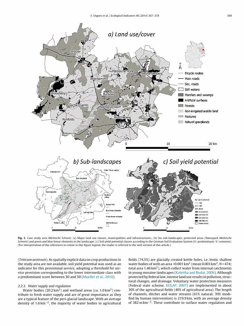

F. Ungaro et al. / Ecological Indicators 46 (2014) 367–378 369

Fig. 1. Case study area Märkische Schweiz. (a) Major land use classes, municipalities and infrastructures.; (b) Six sub-landscapes, protected areas (Naturpark MärkischeS l class( erred

(tiva

2

tad

chweiz) and green and blue linear elements in the landscape; (c) Soil yield potentiaFor interpretation of the references to colour in this figure legend, the reader is ref

Triticum aestivum). As spatially explicit data on crop productions inhe study area are not available, soil yield potential was used as anndicator for this provisional service, adopting a threshold for ser-ice provision corresponding to the lower intermediate class with

predominant score between 30 and 50 (Mueller et al., 2010).

.2.3. Water supply and regulation

Water bodies (20.2 km2) and wetland areas (ca. 1.0 km2) con-

ribute to fresh water supply and are of great importance as theyre a typical feature of the peri-glacial landscape. With an averageensity of 1.6 km−2, the majority of water bodies in agricultural

es according to the German Soil Evaluation System (U: predominant; V: common).to the web version of this article.)

fields (74.5%) are glacially created kettle holes, i.e. lentic shallowwater bodies of with an area <0.001 km2 (mean 0.003 km2, N = 474;total area 1.46 km2), which collect water from internal catchmentsin young moraine landscapes (Kalettka and Rudat, 2006). Althoughprotected by federal law, intense land use results in pollution, struc-tural changes, and drainage. Voluntary water protection measures(Federal state scheme, KULAP, 2007) are implemented in about

30% of the agricultural fields (40% of agricultural area). The lengthof channels, ditches and water streams (61% natural; 39% modi-fied by human intervention) is 219.9 km, with an average densityof 382 m km−2. These contribute to surface water regulation and

370 F. Ungaro et al. / Ecological Indicators 46 (2014) 367–378

Table 1Landscape elements, spatial characteristics and data sources used to identify the landscape services addressed in this paper.

Landscape elements/spatialcharacteristics

Landscape service Categories ofservices

Data source

Soil typeYield potential

Crop production (PRO) Provision Bundesanstalt für Geowissenschaften und Rohstoffe:Bodenübersichtskarte 1:200.000 (BÜK 200)

Land use Crop production (PRO) Provision Corine Land Cover 2006, European Environment AgencyDigitales Feldblockkataster (DFBK) des LandesBrandenburg 2012

Field sizeArea designation

Habitat for species (HAB) Supporting Digitales Feldblockkataster (DFBK) des LandesBrandenburg 2012

Group of trees and single treeshedgerows, tree lines, alleys

Habitat for species (HAB)Visual appreciation and inspirationfor culture, art and design (VIS)

SupportingCultural

Biotopkartierung Brandenburg–Liste der Biotoptypen mitAngaben zum gesetzlichen Schutz (§32 BbgNatSchuG), zurGefährdung und zur Regenerierbarkeit 2011

ProviRegulCultu

gc

2

hoMellaetiNars2

2a

tn1sweo

i

tsswbtTarsost

Wetlands, Marshes and ponds,Streams, small rivers, ditches

Water storage and supply (WAS)Water regulation (WAR)Habitat for species (HAB)

roundwater control, providing habitat for species and offeringultural services.

.2.4. Visual appreciationGreen linear elements, such as tree rows, tree alleys and

edgerows with a total length of 268 km and an average densityf 1,017 m km−2 are a key feature of the agrarian landscape of theärkische Schweiz. Alleys and tree rows represent the dominant

lement type with a share of nearly 50% of the total length, fol-owed by hedgerows and windbreaks representing 39% of the totalength. Other landscape elements such as woodlots and fruit treesccount for the remaining share of 11.5%. The presence of theselements results in a half-open agricultural landscape of high aes-hetic value, which is highly appreciated by tourists and valued asntegral part of the regional identity by residents (Häfner, 2014).evertheless, scale enlargement and increasing land use intensityre currently affecting the spatial structure and composition of theural landscapes, often associated with the risk of removal of land-cape elements following increases of field plot sizes (Stoate et al.,009).

.3. Characterisation of spatial pattern of landscape structuresnd services

In order to characterise the heterogeneity and spatial pat-erns of the diverse landscape elements and related services, aon-parametric probabilistic approach has been adopted (Journel,983). Within this framework the information about the provi-ion of a given landscape service at any given position u˛ = (x˛, y˛)ithin the landscape can take the form of an indicator i(u˛) of pres-

nce/absence of the service at that point of coordinates x˛ and y˛

r within a buffer around it:

(u˛) ={

1 if the landscape service is provided

0 otherwise(1)

The area was divided into grid cells of 1 km2 within whichwo random points were set, representing the sites at which theelected landscape elements and services were assessed. Thistratified random sampling design led to a total of 1344 points,ith an average sampling density equal to 2.3 km−2. At each point,

uffers of different size, ranging from 125 to 500 m, were appliedo assess the presence or absence of specific landscape features.he buffer size depended upon the spatial extent of the servicend on the type of data required for the assessment: (i) one-to-oneelation to land cover or to soil type; (ii) single data source (e.g.,

ingle landscape element); (iii) multiple data sources (e.g. sharef area under protection schemes at field scale). Different bufferizes around the sampling points were tested, ranging from 125o 500 m, with increasing steps of 125 m. For all the considered

sionationral

Biotopkartierung Brandenburg–Liste der Biotoptypen mitAngaben zum gesetzlichen Schutz (§32 BbgNatSchuG), zurGefährdung und zur Regenerierbarkeit 2011

landscape elements a buffer size of 250 m around sampling pointswas eventually selected. An increase in buffer size decreasesspatial resolution, while smaller buffers do not intercept enoughelements to catch and model their spatial structure and hence failto properly detect the existing variability. In the case of habitat(HAB) and production services (PRO), values were taken at thepoints, as the available information in these two cases is referredto polygonal objects, i.e. field plots and soil units, respectively.

For each of the selected services an indicator dataset was thencreated and experimental semivariograms were used to charac-terise its spatial pattern. The indicator variogram is computed asthe half of the expected squared increment of the values betweenlocations u˛ and u˛+h:

�̂I(h) = 12N

N(h)∑˛=1

[i(u˛) − i(u˛+h)]2 (2)

where N(h) is the number of pairs within a given spatial distance(and direction) known as lag h and i(u˛) and i(u˛+h) the value ofthe indicator variable at locations u˛ and u˛+h, respectively. Theexperimental variogram provides only an empirical description ofthe spatial distribution of a given landscape structure or element.A model fitted to the experimental values, i.e. a valid mathemati-cal function, is then necessary to provide a parametric descriptionof the spatial heterogeneity components (Wackernagel, 2003). Theparameters of a variogram model are: (i) its intercept on the y-axis,called nugget (C0) which accounts for uncorrelated spatial noise orfor spatial structures not detected at the scale of investigation; (ii)a sill (C1) which is the spatially structured variance; and (iii) therange (r), i.e. the distance at which the variogram reaches its sill.In the presence of spatial clusters of provision of a service, the var-iogram value is expected to increase with distance h and to reacha plateau, the sill, at a range, corresponding to the average size ofthese clusters. Data separated by a distance larger than the rangeare uncorrelated.

To account for multiple scales in data variability linear com-bination of these models can be used, resulting in nested modelsemivariogram model. A nested variogram model is the weightedsum of n elementary models and is suitable to describe specific setsof spatial structures, over imposed in the same area and each relatedto a different spatial scale. As such it is appropriate to describe thetwo components of spatial heterogeneity in any given landscape: (i)the overall degree of landscape heterogeneity expressed by a givenlandscape element, given by the total sill �2, and (ii) the spatialstructure of any given element, characterised by the parameters of

the model, i.e. its ranges rn and fractions of the total sill fn relatedto each range.

The experimental indicator semivariograms were calculatedassuming a lag, i.e. an incremental step over the distance, equal to

l Indic

4smm

2p

psfmpoi

p

welalItnaAobatpp2(p

3

3

ipad

sietcwl

ttata3as

F. Ungaro et al. / Ecologica

00 m, as this distance proved to return in all cases experimentalemivariogram functions regularly increasing with distance. Theaximum distance was set to 12,000 m, i.e. about half the maxi-um width of the area.

.4. Mapping single and joint probability of landscape serviceotential supply

Based on the variogram models, the probability of servicerovision has been mapped via conditional sequential indicatorimulations (SIS). A detailed introduction on the SIS method can beound in Goovaerts (1997) and has been widely applied to address

any environmental issues. The estimate conditional probabilityk* of occurrence of a given service supply is calculated at the nodesf a regular grid u0 as the linear combination of the n neighbouringndicator data i(u˛):

∗k (u0) =

n∑˛=1

�˛ (u0) × i (u˛) (3)

here the weights �˛ are obtained by solving the system of lin-ar equations known as the ordinary kriging system. For eachandscape service, 1000 simulation outcomes have been generatedt the node of a 100 m square grid for a total of 57,657 simu-ated values for each realisation over the entire area (576.57 km2).n post-processing the simulation outcomes, the E-type estima-or (Deutsch and Journel, 1998) was calculated at each simulationode, i.e. the mean probability of service provision p*E(u0) within

buffer around a given grid node given n conditional observations.ssuming they are independent, the joint probability of occurrencef any couple of services LS1 and LS2 at any given position uo cane calculated as the products of their single probabilities p∗

ELS1 (u0)nd p∗

ELS2 (u0) at the same location. Joint probability values can behen used to assess the presence of hot or cold spots of services sup-ly in the study area. All the geostatistical analyses presented in thisaper were carried out with the software Wingslib 1.3.1 (Statios,000), which works in conjunction with the GSLIB90 executablesDeutsch and Journel, 1998). All GIS operations and mapping wereerformed using QGIS v1.8.0. (QGIS Development Team, 2012).

. Results

.1. Spatial structure of landscape services

Fig. 2 indicates the location of the sampling points and thendicator coding for each service, while Table 2 summarises theotential services supply as observed at the 1344 sampling pointsnd expressed in terms of probability of occurrence and its standardeviations.

The experimental indicator variograms for the five services arehown in Fig. 3 along with the models fitted to them. Nested spher-cal models with a nugget component provided the best fit to thexperimental variograms which are all characterised by discon-inuity at the origin, linear behaviour with change of slope andonvergence to a sill. In all cases a nugget and two componentsell described the experimental data, only in the case of the green

inear element (VIS) a third component was added (Table 3).The quote of unresolved variability ranges from 4 to 20% of the

otal sill, with the minimum observed for water supply (WAS) andhe maximum for habitat provision (HAB). All the services are char-cterised by at least two superimposed scales of spatial variation:he smaller one ranges from 1056 m (WAS) to 2200 m (PRO) and

ccounts for a share of spatially structured variation ranging from6% (HAB) to 71% (WAS); the greater one ranges from 3500 m (VISnd WAR) to 6900 m (PRO) and accounts for a share of spatiallytructured variability ranging from 24% (WAR) to 44% (HAB). A third

ators 46 (2014) 367–378 371

component over a range of 12,000 m accounts for 14% of the spa-tially structured variability observed for the visual appreciation ofgreen linear elements.

3.2. Mapping single and joint probabilities of landscape servicesupply

Using the variogram models, the probability of occurrence ofthe selected landscape services have been mapped over a regular100 × 100 m grid via sequential indicator simulation with ordinarykriging. The spatial distributions of mean simulated probabilitiesare presented in Fig. 4. The maps of the E-type estimates clearlyreveal distinctly different spatial patterns of the seven landscapeservices. Water regulation services (WAR; mean 0.15; std. dev.0.26) occur typically in localised clusters scattered in the wholearea; five distinct large clusters can be observed, the largest ofwhich in the south–west of the area corresponding to the glacialvalley of the Rotes Luch. Habitat provision services (HAB; mean0.36; std. dev. 0.35) are mainly clustered around the core of thecase study area, but spots of high service supply also occur in itsnorth-eastern and south-eastern fringes. Areas with high visualappreciation (VIS; mean 0.30; std. dev. 0.32) are similarly clusteredaround the central protected area but the clusters on the easternpart of the area are smaller and less contiguous. Provision concen-tration of water supply services (WAS; mean 0.32; std. dev. 0.32) arefound mainly in the south–east and north–west, while the oppo-site is observed for crop provision services (PRO; mean 0.74; std.dev. 0.27) which, although rather ubiquitous, are clearly clusteredin the north-eastern and in the south-western parts of the area.The highest probability is that referring to crop provision services(mean 0.74), as most of the agricultural fields occur in high yieldpotential areas. With the exception of habitat for species (mean0.36) and water regulation (mean 0.32) all the selected servicesshow a mean probability of occurrence <0.30. Most of the simu-lated E-type distributions are strongly asymmetric and positivelyskewed, with values >1 observed for WAR (skewness 1.85). Themaps of the potential supply of this service are indeed characterisedby well-defined local clusters of high values.

The differences in the spatial distribution of the potential supplyof the single services can eventually be summarised and visualisedfor each of the six sub-landscapes, highlighting the differences inallocations of the selected services as depending upon landscapestructure and composition. The web charts in Fig. 5 depict thetrade-offs between the selected landscape services: three out ofsix sub-landscapes (Lebus Plateau and Oberbarnim, and the RiverOder Valley) are strongly oriented towards the provision of onesingle service, i.e. crop provision (PRO), while in the other threelandscapes a joint supply of diversified services is observed. In thesub-landscape of the Barnim Plateau, PRO is still the dominant ser-vice, nevertheless substantial supply of VIS, HAB and WAS servicesis observed. In the case of the glacial valley of Rotes Luch, HAB andWAR supplies are nearly equal to PRO, while in the case of the otherglacial valley, i.e. the Buckow Valley, the supply of WAS is more pro-nounced of PRO, followed by a substantially equivalent provisionof VIS and HAB services.

In terms of correlation between services pairs, VIS andHAB exhibit the highest significant (p < 0.01) positive correlation(r = 0.54), followed by those between VIS and WAR (r = 0.35), andHAB and WAR (r = 0.25). However, these are general trends andlocal clusters of high occurrence of both services, leading to syn-ergies or conflicts, cannot be excluded based on these results. Theexistence of different bundles of services with synergies and con-

flicts is then only suggested by the sign and the strength of thecorrelation, but their joint supply can be better elucidated mappingthe joint probability of occurrence of different pairs of services. Thedescriptive statistics of the global joint probability of occurrence of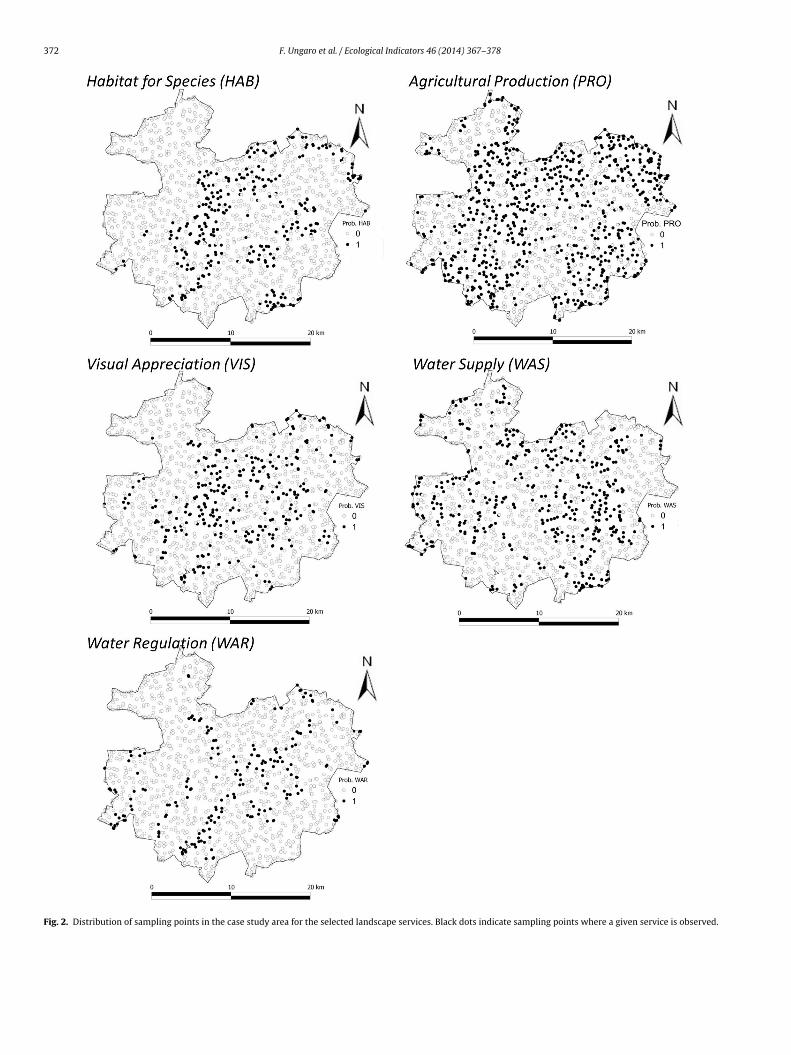

372 F. Ungaro et al. / Ecological Indicators 46 (2014) 367–378

Fig. 2. Distribution of sampling points in the case study area for the selected landscape services. Black dots indicate sampling points where a given service is observed.

F. Ungaro et al. / Ecological Indicators 46 (2014) 367–378 373

Table 2Potential services supply within buffer centred around 1344 sampling points: mean probabilities of occurrence and standard deviations.

Landscape service Buffer size (m) Intercepted elements Probability of occurrence Standard deviation

Habitat for species (HAB) At point 285 0.212 0.409Agricultural production (PRO) At point 711 0.533 0.499Visual appreciation (VIS) 250 290 0.216 0.412Water regulation (WAR) 250 201 0.150 0.357Water supply (WAS) 250 440 0.327 0.469

Table 3Semivariogram model parameters for the five selected landscape services. For all services, the parameters refer to nested spherical semivariogram models. The spherical

semivariogram model can be written as: � (h) = C0 +n∑

i=1

Ci

(1.5h/ri − 0.5h3/r3

i

), for h ≤ ri , where h is the distance (m), C0 is the nugget, Ci (i = 1,. . ., n) the sill of the i

nested structure, and ri its spatial range (m). Std.: parameter values standardised over total sill and expressed as percentages of total sill. HAB: habitat for species; PRO:agricultural production; VIS: visual appreciation; WAR: water regulation; WAS: water supply.

Model type HAB PRO VIS WAR WAS

Nugget, C0 0.033 0.020 0.027 0.011 0.012Std. 20.0% 15.3% 16.0% 9.0% 4.0%Sill 1 C1 Spherical 0.060 0.065 0.076 0.084 0.153Std. 36.0% 49.7% 45.0% 67.0% 71.0%Sill 2 C2 Spherical 0.074 0.045 0.042 0.030 0.051Std. 44.0% 34.4% 25.0% 24.0% 26.0%Sill 3 C3 Spherical 0.02Std. 14.0%Range 1 (m) 1700 2200 1100 1500 1056Range 2 (m) 5700 6900 3500 3500 4422Range 3 (m) 12000

Total sill 0.167 0.130 0.170 0.126 0.216Observed variance 0.167 0.131 0.170 0.126 0.215

Table 4Mean joint probability values and standard deviations (in brackets) for the occurrence of pairs of selected landscape services for the whole case study area under agriculturalland uses. (N = 26,390). HAB: habitat for species; PRO: agricultural production; VIS: visual appreciation; WAR: water regulation; WAS: water supply.

Landscapes services HAB PROD VIS WAR WAS

HAB –PROD 0.279 (0.310) –VIS 0.166 0.228

WAR 0.076 (0.166) 0.111 (0.207)WAS 0.076 (0.166) 0.233 (0.266)

Fig. 3. Experimental indicator semivariograms for the occurrence of the selectedlandscape services. HAB: Habitat for species; PRO: agricultural production; VIS:visual appreciation; WAR: water regulation; WAS: water supply.

–0.112 (0.187) –0.112 (0.187) 0.055 (0.142) –

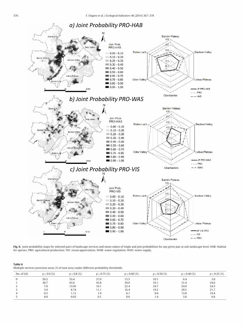
any given couple of landscape services are shown in Table 4. Thehighest mean join probability is that observed for the joint sup-ply of PRO and HAB services (0.28), followed by those for PRO andWAS (0.23) and PRO and VIS (0.22). These findings highlight theoccurrence of hotspots of service provision with possible conflictsbetween the on-going intensification of agricultural management,often associated to field enlargement and to the removal of land-scape elements, and the maintenance of landscape features such astree elements or kettle holes, which underpin the delivery of ser-vice others than food provision. Mean global join probabilities >0.1are observed for the following pairs of landscape services: HAB-VIS(0.17), PRO-WAR (0.11), VIS-WAR (0.11) and VIS-WAS (0.11).

These global figures refer to the whole study area, whereas formanagement and planning purposes it is more relevant to identifythe local differences in joint services provision, which can be madevisually explicit in join probability maps. The joint probability forthree couples of selected services along with their average in thesix sub-landscape of the area is illustrated in Fig. 6. The maps showclearly the extent and the degree of the spatial co-occurrence forspecific couples of services, i.e. hotspots of service supply as result-ing from the interplays between the specific pairs of indicators.The joint supply of provision and habitat services (Fig. 6a) is par-

ticularly relevant in the Rotes Luch, where a majority of the fieldsare under protection schemes. Hotspots of high joint probability ofPRO and WAS (Fig. 6b) and VIS (Fig. 6c) services are concentratedin the Barnim Plateau and to some extent in the Buckow Valley and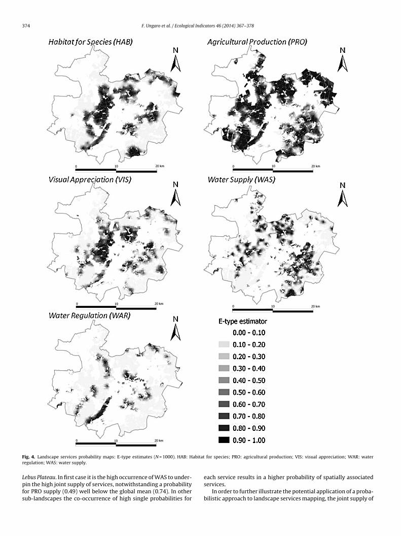

374 F. Ungaro et al. / Ecological Indicators 46 (2014) 367–378

F abitatr

Lpfs

ig. 4. Landscape services probability maps: E-type estimates (N = 1000). HAB: Hegulation; WAS: water supply.

ebus Plateau. In first case it is the high occurrence of WAS to under-in the high joint supply of services, notwithstanding a probabilityor PRO supply (0.49) well below the global mean (0.74). In otherub-landscapes the co-occurrence of high single probabilities for

for species; PRO: agricultural production; VIS: visual appreciation; WAR: water

each service results in a higher probability of spatially associatedservices.

In order to further illustrate the potential application of a proba-bilistic approach to landscape services mapping, the joint supply of

F. Ungaro et al. / Ecological Indicators 46 (2014) 367–378 375

F of thea

dusotbepm

4

osafi2lp

TSr

ig. 5. Trade-offs between the five landscape services in the six sub-landscapesppreciation; WAR: water regulation; WAS: water supply.

ifferent couple of services has been calculated for paired servicesnder different probability thresholds. The occurrence of possibleervices bundles is presented in Table 5, which identifies the areasf joint coupling of services and their ranks under the differenthresholds. The stability of the results of the analysis is confirmedy the fact that the ranks are nearly the same under the differ-nt thresholds. As multiple service areas decrease with increasingrobabilities, the optimal threshold should be selected by decisionakers based on their specific targets.

. Discussion

The adoption of spatially explicit approaches to the assessmentf ecosystem services allows for a better integration of landscapeervices in agricultural systems management (Frank et al., 2012),nd examples can be found in recent literature ranging from the

eld (Rutgers et al., 2012) to national scales (van Wijnen et al.,012). Applications of geostatistical methods to quantify and map

andscape services over catchments and regions have, not unex-ectedly, mostly focused on soil ecosystem services within the

able 5ervice bundles areas (% of total area) under different probability thresholds. HAB: habitegulation; WAS: water supply.

Joint services p ≥ 0.9 p ≥ 0.8 p ≥ 0.75 p ≥ 0.60

Area (%) Rank Area (%) Rank Area (%) Rank Area (%)

PRO-HAB 5.7 1 11.8 1 15.5 1 26.1

PRO-VIS 4.5 2 8.5 2 10.5 2 17.9

WAS-PRO 2.8 4 7.4 3 9.8 3 17.8

HAB-VIS 3.2 3 6.5 4 7.9 4 14.1

WAS-HAB 1.4 5 3.5 5 5.0 5 10.3

PRO-WAR 1.0 6 3.1 6 4.4 6 8.0

WAS-VIS 0.5 7 1.7 8 2.5 7 6.7

VIS-WAR 0.5 8 1.8 7 2.4 8 5.3

HAB-WAR 0.2 10 1.2 9 2.2 9 5.3

WAS-WAR 0.3 9 1.0 10 1.5 10 3.3

study area. HAB: Habitat for species; PRO: agricultural production; VIS: visual

landscape, e.g. flood mitigation (Jiang et al., 2007), water storageand regulation (Forouzangohar et al., 2014; Ungaro et al., 2014),and carbon sequestration (Ungaro et al., 2010; Kumar and Lal, 2011;Zhang et al., 2011; Forouzangohar et al., 2014). The approach pre-sented in this paper allows to sample, model and (jointly) mapservices related to other landscape components, further adaptingthe geostatistical conceptual framework in order to maintain orenhance the provision of priority landscape services within a givenarea, identifying in probabilistic terms the locations where avail-able resources could be better targeted.

4.1. Probability thresholds of service hotspots

The presented approach allows for an explicit assessment ofuncertainty associated to the estimates of landscape services: this iscurrently a limitation of many studies on landscape or ecosystem

services which causes major concerns (Johnson et al., 2012; Houet al., 2013). The results displayed as probability maps for eachservice or as joint probability of any desired number of servicesare easily readable and comparable. Geostatistical simulations can

at for species; PRO: agricultural production; VIS: visual appreciation; WAR: water

p ≥ 0.50 p ≥ 0.40 p ≥ 0.25 Avg Var

Rank Area (%) Rank Area (%) Rank Area (%) Rank

1 32.4 1 38.8 1 47.7 1 1.0 0.002 23.8 3 30.8 2 40.4 3 2.3 0.243 23.9 2 30.8 3 41.7 2 2.9 0.484 18.7 4 24.0 4 31.9 4 3.9 0.145 14.0 5 18.0 5 25.9 5 5.0 0.006 10.6 6 13.8 7 19.7 7 6.3 0.247 10.0 7 14.6 6 23.2 6 6.9 0.489 7.5 8 10.7 8 15.8 9 8.1 0.488 7.5 9 10.5 9 16.0 8 8.9 0.48

10 4.8 10 7.0 10 11.6 10 9.9 0.14

376 F. Ungaro et al. / Ecological Indicators 46 (2014) 367–378

Fig. 6. Joint probability maps for selected pairs of landscape services and mean values of single and join probabilities for any given pair at sub-landscape level. HAB: Habitatfor species; PRO: agricultural production; VIS: visual appreciation; WAR: water regulation; WAS: water supply.

Table 6Multiple services provision areas (% of total area) under different probability thresholds.

No. of LSS p ≥ 0.9 (%) p ≥ 0.8 (%) p ≥ 0.75 (%) p ≥ 0.60 (%) p ≥ 0.50 (%) p ≥ 0.40 (%) p ≥ 0.25 (%)

0 50.2 33.4 27.0 15.5 10.1 6.4 3.01 38.7 43.6 43.8 39.0 35.1 31.4 24.62 7.0 13.05 16.1 22.4 24.7 24.9 24.53 3.9 8.74 11.1 16.4 19.2 20.5 21.74 0.3 1.11 1.9 6.1 9.6 13.8 19.45 0.0 0.03 0.1 0.6 1.4 3.0 6.8

l Indic

babpsaoTafpudvsas

fccfipaap

4

sattottutst

sfawtrttttv

crtotsitsabs

F. Ungaro et al. / Ecologica

e viewed as the spatial counterpart of Monte Carlo simulation;s such a significant number of simulations are required for sta-le results and to reproduce the statistical features of the sampledopulation, i.e. its histogram and its semivariogram. In doing so,imulations also provide a tool to assess and map the uncertaintybout the simulated values. Setting of different probability thresh-lds supports identification of hotspots of multiple services supply.able 6 summarises the delivery of a growing number of servicesssuming different probability thresholds of services occurrenceor the whole agricultural area (263.9 km2). For example setting arobability threshold of service occurrence >0.50, 10% of the areander agricultural land uses provides no landscape services, 35%elivers one service while 25% and 19% supply two and three ser-ices, respectively. The shares of agricultural area with a potentiallyupply of four services jointly is equal to 10%, while only 1.4% of therea has a potential to deliver the considered five joint landscapeervices.

The geostatistical simulation results have been presented at aollow-up stakeholder workshop in February 2014. The identifiedonflict areas between the (intensified) crop production, natureonservation and tourism development objectives have been con-rmed being particularly immanent at the fringes of the naturearks core area. Those have been discussed as specific spaces ofction for landscape regulation to cope with the scale enlargementnd the clearance of landscape elements, such as green linear andoint elements as well as kettle holes.

.2. Advantages and limitations of the approach

The transfer of the presented approach to other conditions andcales is immediate if spatially explicit data on landscape elementsre available as the size of the sampling grid and the number ofhe sampling points can be adapted to any scale of interest. Addi-ional landscape elements can easily be integrated if available andf interest in terms of their capability to represent valid indica-ors of service supply in a new specific context. The selection ofhe indicators is a crucial aspect of this approach as they underpinnique pattern-process relationships with the landscape serviceshey are meant to infer. The sensitivity of the approach is thentrongly linked to the choice of proper indicators as it relies uponhe modelling of their specific spatial structures.

A noteworthy aspect of the approach is that framing land-cape services provision within a probabilistic framework allowsor an explicit uncertainty assessment, although not distinguishingmong its different sources. Furthermore the probabilistic frame-ork does not require any further standardisation of results as all

he services are assessed in terms of probability of occurrence, i.e.anging from 0 to 1, which are in turn based on meeting the cri-eria defined for the indicators of their potential supply. Thereforehe joint probability calculation represents a straightforward toolo provide a valuable integration to approaches based on propor-ional overlap (Wu et al., 2013), weighting scheme (Gimona andan der Horst, 2007), or relative capacity (Baral et al., 2013).

A substantial aspect of the presented methodology is thehoice of the optimal buffer size around sampling points, whichequires careful consideration of both case-specific objectives andhe nature of spatial characteristics of the elements observed. Inrder to assess their effect on the spatial structure as described byhe experimental semivariograms, we tested four different bufferizes, ranging from 125 to 500 m. Increasing buffer sizes resultn a spatial structure which is more continuous over the two (orhree) superimposed scales of variations. With increasing buffer

ize it is possible to obtain a more precise quantification of thectual spatial scale of the process, but this is counterbalancedy a smoothing effect over shorter distances where variogramsuggest a higher degree of spatial continuity which is actually

ators 46 (2014) 367–378 377

not observed in reality. The actual degree of spatial correlation atshort distances is indeed better described by the smaller buffersconsidered, while large scale correlation are similarly detected andreproduced at any buffer size. With smaller buffers, the probabilityassociated to the random points is lower than the observed dueto lack of intercepted elements within the buffer which in turnresults in a general underestimation. The opposite is observedfor larger buffers, where more elements are intercepted resultingin a general overestimation, i.e. high probability of landscapeservices where actually they do not occur. The “optimal” buffersize requires balancing of these two contrasting effects.

5. Conclusion

In this study the spatial structures of five landscape servicesin a multifunctional agricultural landscape in North-East Germanyare modelled and mapped resorting to a probabilistic approachusing sequential indicator simulations. The proposed methodologyis of general applicability and can be implemented wherever basicgeoreferenced information on landscape elements is available. Atthe landscape level, variogram analysis allows the characterisationand the synthesis of the spatial heterogeneity and of the spatialranges of landscape elements and related services. This approachhighlights and explicitly quantifies the differences in the spatialstructure of the selected services. The choice of the optimal buffersize for service sampling and variogram calculation is not straight-forward and depends mainly on the objective pursued and on thenature of the elements observed. The decrease of spatial resolution(i.e. increase in buffer size) nevertheless is not associated to a lossof spatial variability and data regularisation seems to affect onlyshort range variability. Probability maps provide a straightforwardvisualisation tool to explore the impact of one or more continu-ous or ordered categorical covariates on the likelihood of singleor joint landscape services potential supply The approach allowsfor a spatially explicit assessment of services co-occurrence at anygiven location within a landscape. The assessment of service rich-ness can be made at different aggregation levels and under differentprobability thresholds in order to support different stakeholder inplanning and decision making.

Acknowledgments

This study was supported by the EU 7th Framework Programproject CLAIM (Supporting the role of the Common agriculturalpolicy in LAndscape valorisation: Improving the knowledge base ofthe contribution of landscape Management to the rural economy)funded by the European Commission-DG Research & Innovation(Call Identifier: FP7-KBBE.2011.1.4-04; Grant Agreement Number222738). The authors wish to thanks the anonymous reviewerswhose valuable comments improved the original version of themanuscript.

References

Anton, C., Young, J., Harrison, P., Musche, M., Bela, G., Feld, C.K., Harrington, R.,Haslett, J.R., Pataki, G., Rounsevell, M.D.A., Skourtos, M., Sousa, J.P., Sykes, M.T.,Tinch, R., Vandewalle, M., Watt, A., Settele, J., 2010. Research needs for incorpo-rating the ecosystem service approach into EU biodiversity conservation policy.Biodivers. Conserv. 19 (10), 2979–2994.

Bagstad, K.J., Semmens, D.J., Waage, S., Winthrop, R., 2013. A comparative assess-ment of decision support tools for ecosystem services quantification andvaluation. Ecosyst. Serv. 5, 27–39.

Baral, H., Keenan, R.J., Fox, J.C., Stork, N.E., Kasel, S., 2013. Spatial assessment ofecosystem goods and services in complex production landscapes: a case study

from south-eastern Australia. Ecol. Complexity 13, 35–45.

Burkhard, B., Kroll, F., Nedkov, S., Müller, F., 2012. Mapping ecosystem service supply,demand and budgets. Ecol. Indic. 21, 17–29.

Brown, K.A., Johnson, S.E., Parks, K.E., Holmes, S.M., Ivoandry, T., Abram, N.K., Del-more, K.E., Ludovic, R., Andriamaharoa, H.E., Wyman, T.M., Wright, P.C., 2013.

3 l Indic

B

C

d

D

E

E

F

F

F

G

G

G

H

H

H

H

H

H

H

J

J

J

J

K

K

K

K

78 F. Ungaro et al. / Ecologica

Use of provisioning ecosystem services drives loss of functional traits acrossland use intensification gradients in tropical forests in Madagascar. Biodivers.Conserv. 161, 118–127.

ryan, B.A., Crossman, N.D., 2013. Impact of multiple interacting financial incentiveson land use change and the supply of ecosystem services. Ecosyst. Serv. 4, 60–72.

hilès, J.-P., Delfiner, P., 1999. Geostatistics: Modelling Spatial Uncertainty. Wiley,New York, NY.

e Groot, R.S., Alkemade, R., Braat, L., Hein, L., Willemen, L., 2010. Challenges inintegrating the concept of ecosystem services and values in landscape planning,management and decision making. Ecol. Complexity 7 (3), 260–272.

eutsch, C.V., Journel, A.G., 1998. GSLIB, Geostatistical Software Library and User’sGuide, second ed. Oxford University press, New York, NY.

EA, 2007. CORINE land cover 2006 technical guidelines. In: EEA Technical ReportNo 17/2007. European Environment Agency, Copenhagen, 70 pp.

goh, B., Reyers, B., Rouget, M., Richardson, D.M., Le Maitre, D.C., van Jaarsveld,A.S., 2008. Mapping ecosystem services for planning and management. Agric.Ecosyst. Environ. 127, 135–140.

agerholm, N., Käyhkö, N., Ndumbaro, F., Khamis, M., 2012. Community stakehold-ers’ knowledge in landscape assessments–mapping indicators for landscapeservices. Ecol. Indic. 18, 421–433.

orouzangohar, M., Crossman, N.D., MacEwan, R.J., Wallace, D.D., Bennett,L.T., 2014. Ecosystem services in agricultural landscapes: a spatiallyexplicit approach to support sustainable soil management. Sci. World J.,http://dx.doi.org/10.1155/2014/483298.

rank, S., Fürst, C., Koschke, L., Makeschin, F., 2012. A contribution towards a trans-fer of the ecosystem, service concept to landscape planning using landscapemetrics. Ecol. Indic. 21, 30–38.

imona, A., van der Horst, D., 2007. Mapping hotspots of multiple landscape func-tions: a case study on farmland afforestation in Scotland. Landscape Ecol. 22,1255–1264.

oovaerts, P., 1997. Geostatistics for Natural Resources Evaluation. Oxford Univer-sity Press, New York, NY.

ulickx, M.M.C., Verburg, P.H., Stoorvogel, J.J., Kok, K., Veldkamp, A., 2013. Mappinglandscape services: a case study in a multifunctional rural landscape in TheNetherlands. Ecol. Indic. 24, 273–283.

äfner, K., 2014. Assessing cultural ecosystem services: a visual choice experimenton agricultural landscape preferences from a user perspective in the case studyMärkische Schweiz, Germany. In: Master Thesis. Universität Potsdam, Potsdam.

aines-Young, R., Potschin, M., Kienast, F., 2012. Indicators of ecosystem servicepotential: mapping marginal changes and trade-offs at European scales. Ecol.Indic. 21, 39–53.

ein, L., Vankoppen, K., de Groot, R.S., van Ierland, E., 2006. Spatial scales, stakehold-ers and the valuation of ecosystem services. Ecol. Econ. 57, 209–228.

ermann, A., Knutter, M., Hainz-Renetzeder, C., Konkoly-Gyuró, E., Tirászi, A., Bran-denburg, C., Allex, B., Ziener, K., Wrbka, T., 2014. Assessment framework forlandscape services in European cultural landscapes: an Austrian Hungarian casestudy. Ecol. Indic. 37A, 229–240.

offmann, J., 1993. Farn- und Blütenpflanzen in der Märkischen Schweiz: Liste derPflanzenfamilien und Pflanzenarten mit kurzer Einführung zum Untersuchungs-gebiet und Häufigkeitsstufung aller Arten. Eggersdorf: Tastomat.

offmann, J., 2006. Flora des Naturparks Märkische Schweiz. Cuvillier Verlag, Göt-tingen.

ou, Y., Burkhard, B., Müller, F., 2013. Uncertainties in landscape analysis andecosystem service assessment. J. Environ. Manage. 2013 (127, Supplement),S117–S131.

ensen, O.P., Christman, M.C., Miller, T.J., 2006. Landscape-based geostatistics a casestudy of the distribution of blue crab in Chesapeake Bay. Environmetrics 17,605–621.

iang, M., Lu, X.-G., Xu, L.-S., Chu, L.-J., Tong, S., 2007. Flood mitigation benefit ofwetland soil—a case study in Momoge National Nature Reserve in China. Ecol.Econ. 61, 217–223.

ohnson, K.A., Polasky, S., Nelson, E., Pennington, D., 2012. Uncertainty in ecosys-tem services valuation and implications for assessing land use tradeoffs: anagricultural case study in the Minnesota River Basin. Ecol. Econ. 79, 71–79.

ournel, A.G., 1983. Non parametric estimation of spatial distributions. Math. Geol.15, 445–468.

alettka, T., Rudat, C., 2006. Hydrogeomorphic types of glacially created kettle holesin NE Germany. Limnologica 36, 54–64.

areiva, P., Tallis, H., Ricketts, T.H., Daily, G.C., Polasky, S., 2011. Natural Capital.Theory and Practice of Mapping Ecosystem Services. Oxford University Press,Oxford.

oschke, L., Fürst, C., Frank, S., Makeschin, F., 2012. A multi-criteria approach for an

integrated land-cover-based assessment of ecosystem services. Ecol. Indic. 21,54–66.

ULAP, 2007. Richtlinie des Ministeriums für Infrastruktur und Landwirtschaftdes Landes Brandenburg zur Förderung umweltgerechter landwirtschaftlicherProduktionsverfahren und zur Erhaltung der Kulturlandschaft der

ators 46 (2014) 367–378

Länder Brandenburg und Berlin. KULAP, Available at the following URL:〈http://www.mil.brandenburg.de/cms/detail.php/bb1.c.213972.de〉.

Kumar, S., Lal, R., 2011. Mapping the organic carbon stocks of surface soils usinglocal spatial interpolator. J. Environ. Monit. 13 (11), 3128–3135.

Lamarque, P., Quétier, F., Lacorel, S., 2011. The diversity of the ecosystem servicesconcept and its implications for their assessment and management. CR Biol. 334(5–6), 441–449.

Lavorel, S., Grigulis, K., Lamarque, P., Colace, M., Garden, D., Girel, J., Pellet, G., Douzet,R., 2011. Using plant functional traits to understand the landscape distributionof multiple ecosystem services. J. Ecol. 99, 135–147.

Maes, J., Egoh, B., Willemen, L., Liquete, C., Vihervaara, P., Schägner, J.P., Grizzetti,B., Drakou, E.G., La Notte, A., Zulian, G., Bouraoui, F., Peracchini, M.L., Braat, L.,Bidoglio, G., 2012. Mapping ecosystem services for policy support and decisionmaking in the European Union. Ecosyst. Serv. 1, 31–39.

Maisel, J.E., Turner, M.G., 1998. Scale detection in real and artificial landscape usingsemivariance analyses. Landscape Ecol. 13, 347–362.

Meynen, E., Schmithüsen, J., 1962. Handbuch der naturräumlichen GliederungDeutschlands, 9. Bundesanstalt für Landeskunde, Lieferung.

MIL, 2012. Digitales Feldblockkataster (DFBK) des Landes Brandenburg. Ministeriumfür Infrastruktur und Landwirtschaft des Landes Brandenburg (MIL), Potsdam(http://www.mil.brandenburg.de/cms/detail.php/bb1.c.223513.de).

MLUR, 2000. Bodenbewertung für Planungs- und Zulassungsverfahren im LandBrandenburg–Abschlußbericht zum Forschungsprojekt im Auftrag des Minis-teriums für Landwirtschaft. In: Umweltschutz und Raumordnung des LandesBrandenburg, Potsdam.

Mueller, L., Schindler, U., Mirschel, W., Shepherd, T.G., Ball, B.C., Helming, K., Rogasik,J., Eulenstein, F., Wiggering, H., 2010. Assessing the productivity functions ofsoils: a review. Agron. Sustain. Dev. 30, 601–614.

QGIS Development Team, 2012. QGIS geographic information system. In:Open Source Geospatial Foundation Project. QGIS Development Team,〈http://qgis.osgeo.org〉.

Rossi, R.E., Mulla, D.J., Journel, A.G., Franz, E.H., 1992. Geostatistical tools for mod-elling and interpreting ecological spatial dependence. Ecol. Monogr. 62 (2),277–314.

Rutgers, M., van Wijnen, H.J., Schouten, A.J., Muldera, C., Kuitenb, A.M.P., Brussaard,L., Breure, A.M., 2012. A method to assess ecosystem services developed fromsoil attributes with stakeholders and data of four arable farms. Sci Total Environ.415, 39–48.

Scholz, E., 1962. Die naturräumliche Gliederung Brandenburgs. Pädagog, Bezirksk-abinett, 93 pp.

Statios, 2000. WinGslib Version 1.3. Statios Software and Services, San Francisco, CA.Stoate, C., Báldi, A., Beja, P., Boatman, N.D., Herzon, I., van Doorn, A., de Snoo, G.R.,

Rakosy, L., Ramwell, C., 2009. Ecological impacts of early 21st century agricul-tural change in Europe—a review. J. Environ. Manage. 91 (1), 22–46.

Syrbe, R.U., Walz, U., 2012. Spatial indicators for the assessment of ecosystem ser-vices: providing, benefiting and connecting areas and landscape metrics. Ecol.Indic. 21, 80–88.

TEEB, 2010. The economics of ecosystems and biodiversity. In: Mainstreaming theEconomics of Nature: A Synthesis of the Approach, Conclusions and Recommen-dations of TEEB. TEEB, Mriehel, Malta.

Termorshuizen, J.W., Opdam, P., 2009. Landscape services as a bridge betweenlandscape ecology and sustainable development. Landscape Ecol. 24,1037–1052.

Ungaro, F., Staffilani, F., Tarocco, P., 2010. Assessing and mapping topsoil organiccarbon stock at regional scale: a scorpan kriging approach conditional on soilmap delineation and land use. Land Degrad. Dev. 21, 565–581.

Ungaro, F., Calzolari, C., Pistocchi, A., Malucelli, F., 2014. Modelling the impact ofincreasing soil sealing on runoff coefficients at regional scale: a hydropedologicalapproach. J. Hydrol. Hydromech. 62 (1), 33–42.

van Wijnen, H.J., Rutgers, M., Schouten, A.J., Mulder, C., de Zwart, D., Breure, A.M.,2012. How to calculate the spatial distribution of ecosystem services—naturalattenuation as example from The Netherlands. Sci. Total Environ. 415, 49–55.

van der Zanden, E., Verburg, P.H., Mücher, C.A., 2013. Modelling the spatial distribu-tion of linear landscape elements in Europe. Ecol. Indic. 27, 125–136.

van Zanten, B., Verburg, P., Espinosa, M., Gomez–Y-Paloma, S., Galimberti, G., Kan-telhardt, J., Kapfer, M., Lefebvre, M., Manrique, R., Piorr, A., Raggi, M., Schaller, L.,Targetti, S., Zasada, I., Viaggi, D., 2013. European agricultural landscapes, com-mon agricultural policy and ecosystem services: a review. Agron. SustainableDev. 1–17, doi: http://dx.doi.org/10.1007/s13593-013-0183-4.

Wackernagel, H., 2003. Multivariate Geostatistics: An Introduction with Applica-tions. Springer, Berlin.

Wu, J., Feng, Z., Gao, Y., Peng, J., 2013. Hotspot and relationship identification in mul-

tiple landscape services: a case study on an area with intensive human activities.Ecol. Indic. 29, 529–537.

Zhang, C.S., Tang, Y., Xu, X.L., Kiely, G., 2011. Towards spatial geochemical modelling:use of geographically weighted regression for mapping soil organic carbon con-tents in Ireland. Appl. Geochem. 26 (7), 1239–1248.