MAPPING CLIMATIC RISKS IN THE EU AGRICULTURE

JAVIER GALLEGO, COSTANZA CONTE, CHRISTOPH DITTMANN, JOSEF STROBLMAIR, MARIA BIELZA

Agrifish Unit, JRC Ispra, Italy Javier.gallego@jrc.it

Paper prepared for presentation at the 101st EAAE Seminar ‘Management of Climate Risks in Agriculture’, Berlin, Germany, July 5-6, 2007

Copyright © European Communities, 2007. All rights reserved. Readers may make verbatim copies of this document for non-commercial purposes by any means, provided that this copyright notice appears on all such copies.

2

MAPPING CLIMATIC RISKS IN THE EU AGRICULTURE

Javier Gallego, Costanza Conte, Christoph Dittmann, Josef Stroblmair and MariaBielza∗

Abstract

Several sources of data have been used to give a geographical picture of the level of risk in the EU agriculture: Yield data from the Eurostat REGIO database, FADN (Farm Accountancy Data Network), agro-meteorological models and satellite images. Most of the maps produced correspond to the crop sector.

Keywords

Agrometeorological models, climatic risk, European Union, vegetation indices,

1. Introduction The agricultural sector is characterised by high exposure to risk. Risks in agriculture can be grouped in two main groups: price risks due to trade liberalisation and production risks due to adverse weather conditions or other reasons (rising quality requirements on animals and plants diseases across borders, etc). Weather is an important production factor in agriculture and is a major source of uncertainty for farms. Perhaps the most obvious impact of weather risk is on crop yields, but its relevance is not limited to crop production. The performance of livestock farms, the turnover of processors, the use of chemicals and fertilizers and the demand for many food products also depend on the weather. Hence, large parts of the agribusiness are affected by weather risks. Producers can try to minimize the negative economic consequences of extreme weather events by using risk management tools, e.g. insurances or other financial instruments. These tools rely heavily on wide range of information like meteorological data, crop specific vegetation data, regional conditions data (soil, topography, etc.) as well as economic data. In the EU the exposure to risks in agriculture, climatic and economic, varies considerably from country to country, therefore the knowledge of local situation plays a key role in assessing the natural hazards and consequently set up the appropriate management tools in order to minimize their impacts. Mapping the meteorological risks on the basis of agro-meteorological models gives the first insight on the impact: which damages, which crops and which areas. Hail, excessive rain, drought, heat waves and frost can be considered as the main climatic events causing damage to crops. The Crop Growth Monitoring System (CGMS) of the MARS Project of the European Commission has been used to map some types of climatic risks. The CGMS uses crop physiology models, a soil map and a climatic database, obtained by interpolation of daily observations in more than 2000 meteorological stations since 1975. The area covered by the system encompasses not only the whole EU but also the Maghreb and the Eastern Europe including large part of European Russia and Caucasian States.

∗ Agrifish Unit, JRC Ispra, Italy.

3

2. Crop Growth Monitoring System (CGMS) The Crop Growth Monitoring System, as a kernel of the MCYFS (Mars Crop Yield Forecast System), developed by MARS Project (Monitoring Agriculture with Remote Sensing) provides the European Commission (DG Agriculture) with objective, timely and quantitative yield forecasts at regional and national scale. The CGMS started as R&D project in the late 80s (GENOVESE, 1994) and became fully operational since 1999. CGMS monitors crops development in Europe, driven by meteorological conditions modified by soil characteristics and crop parameters. This mechanistic approach describes the crop cycle (i.e. biomass, storage organ, etc.) in combination with phenological development from sowing to maturity on a daily time scale. The main characteristic of CGMS lies in its spatialisation component, which integrates interpolated meteorological data, soil and crop parameters, through elementary mapping units used for simulation in the crop model. The core of the system is based on 2 deterministic crop models, WOFOST (VAN DIEPEN et al, 1989, SUPIT et al, 1994) and LINGRA (SCHAPENDONK et al., 1998, RODRIGUEZ et al., 1999) for pastures. GIS tools are used to prepare data and to produce results maps. Input and output are stored in a RDBMS. Statistical procedures are used to forecast quantitative crops yield. In summary, CGMS consists of three main parts: level 1: interpolation of meteorological data into a square grid; level 2: simulation of the crop growth; level 3: statistical evaluation of the results. Figure 1: Flowchart of CGMS

4

2.1 Weather data Daily meteorological station data are used in two ways for crop yield evaluation: first, as weather indicator for a direct evaluation of alarming situations such as drought, extreme rainfall during sowing, flowering or harvest; second, as input for the crop growth model WOFOST. The stations are limited to those for which data not only are regularly collected but which can also be received and processed in semi-real time. As the data are obtained from a variety of different sources, considerable pre-processing is necessary to convert them to a standard format. From 1991 to present, meteorological data are received in near real time from the GTS (Global Telecommunication System) network for different hours within one day. The data are pre-processed and quality checked. Finally, the data is converted into daily values of at least the minimum and maximum daily air temperature, rainfall, wind speed, vapour pressure, as well as either global radiation, sunshine hours or cloud cover. In this way the MARS project has established an up-to-date database of harmonised, quality checked daily data from an network of stations across western and eastern Europe, western Russia, the Maghreb and Turkey. A good coverage is obtained since 1975. The database does not contain evapotranspiration values and some records on measured global radiation. As such information is needed for the agro-meteorological model it is derived from the other available data. Potential evapotranspiration is calculated by the CGMS with the Penman-Monteith formula (MONTEITH, 1985); in cases where global radiation is not recorded, it is derived from sunshine duration, cloud cover and/or temperature. Depending on the availability of meteorological parameters, either the Supit or Ångsrtöm or Hargreaves formulae is used (SUPIT et al., 1994; VAN DER GOOT, 1998). To simulate crop growth CGMS needs to interpolate daily meteorological data towards the centres of a regular climatic grid. For Europe this grid measures 50 by 50 kilometres and amounts to 5625 cells. After interpolation of weather data, a representative spatial schematisation of meteorology, soils, crops and land use can be derived, which is necessary to simulate crop development for different spatial units. The interpolation method was chosen because its simple approach made it easy to automate while the accuracy is sufficient to serve as input to the crop growth model (BEEK ET AL. 1991; VAN DER VOET ET AL. 1994). The interpolation is executed in two steps: first, meteorological stations are selected that have sufficient temporal coverage and similar meteorological conditions compared to the grid cell centre to which their values are interpolated. To assess this similarity, the CGMS uses a scoring algorithm that takes following criteria into account: distance between the station and the grid cell centre, similarity in altitude and distance to the coast between the station and the grid centre, relative position of the station and the grid cell centre with regard to climatic barriers, i.e. mountain ranges. Second, a simple average over one up to four stations is calculated for most of the meteorological parameters, with a correction for the altitude difference between the station and grid cell centre in case of temperature and vapour pressure. A data availability threshold of 80% is applied to weather stations used for the interpolation of meteorological data. This implies that a weather station can have missing data for a number of days. In such cases missing values are substituted with the long-term average of the concerned weather station and day.

2.2 Crop simulation Crop simulation, level 2 of the CGMS, is built around WOFOST model. WOFOST model, developed by SC-DLO and AB-DLO, Wageningen, The Netherlands, is a quantitative deterministic model that can be used to simulate a number of crops, based on sets of crop parameters and management practices, like sowing density, planting date, etc. It takes into account certain soil characteristics and uses daily meteorological data for the calculation of evolution on time of the crop. WOFOST could be described as a ’point’ model in the sense that

5

it performs the calculation for one single point on space/time. It computes the instantaneous photosynthesis, at three depths in the canopy and for three moments of the day. These instant values are then integrated over the depth of the canopy and over the day light period to achieve daily total canopy photosynthesis. After subtracting the maintenance respiration, assimilates are partitioned over the different plant organs as a function of the development stage, witch is calculated by integrating the daily development rate, described as function of temperature. Above-ground dry matter accumulation and its distribution over leaves, steams and grains are simulated from sowing to maturity. The CGMS simulates two production situations: potential and water-limited. The potential situation is only defined by temperature, day length, solar radiation and crop parameters. In the water-limited situation soil moisture determines whether the crop growth is limited by drought stress. Therefore a soil water balance is calculated that applies to a freely draining soil, where groundwater is so deep, that it does not influence the soil moisture content in the rooting zone. In both, the potential and water limited, situations optimal supply of nutrients is assumed and damage caused be pests, diseases and weed is not considered. To apply the crop growth model WOFOST at a larger scale, simulation units where meteorological data, soil characteristics and crop parameters can be assumed homogeneous have to be identified. This spatial schematisation assumes that the simulated crop growth is representative for those units. For this purpose Elementary Mapping Units (EMU’s) are created which results from the intersection of climatic grid cell, soil mapping unit (SMU) and administrative regions using agricultural statistics (NUTS - Nomenclature des Unités Territoriales Statistiques)

2.3 Yield forecasting The main goal of level 1 and 2 within the CGMS was to monitor weather and crop conditions in order to assess the effect of weather on crop conditions, and to make early yield and production estimates per country and/or large region. To this goal the agro-meteorological crop growth simulation model WOFOST was combined with a GIS and a yield prediction routine to form the CGMS. The purpose of level 3, yield forecasting, is to provide the most likely, precise, accurate, scientific, traceable and independent forecasts for the main crops’ yields at EU level taking into account the effect of the climate during the season as early as possible during the cropping campaign (and until harvest). With this third level, the CGMS is enhanced and included into a larger concept which is the MARS Crop Yield Forecasting System (MCYFS). The main role of the MCYFS (level 3) is to provide yield statistics of the major crops at EU and national level, as accurate and timely as possible, while ensuring independence from all external sources of estimates, including the national statistical systems (GENOVESE, 1998). To realise this objective crop yield forecast procedures are applied which combine all kinds of input such as historical yield statistics, weather indicators, simulated crop indicators, remote sensing based vegetation indices, additional information sources and expert knowledge. Time series of historic yield statistics of EUROSTAT are an important data source in this procedure which is mainly based on regressions. In this context the MCYFS assumes that the official yield statistics are objective statistics and reflect the real situation. In order to make the most likely, precise accurate, traceable and independent forecasts for the main crops different statistical tools are used: trend analysis, regression analysis, scenario/similarity analysis. At the end of the process different possible forecasts are available and often “statistically” acceptable. The “most performant result” is then individuated and selected according to statistical tests (DE KONING et al ., 1993) on the models used and scenario analysis results. The measurement error (cause of main bias) is constantly a concern for the MCYFS as this could affect the results of the whole analysis.

6

The geographic dimension of the forecasts given by the MCYFS goes theoretically from the EMU (Elementary Mapping Unit) concept dimension to the Continental dimension passing through the grid cells, regions (NUTS2,1) and country levels. In theory the “predictors” production can be generated at whatever geographic level according to the layer available (catchments boundaries could also be used). In practice, while “predictors” are systematically produced and stored at grid, NUTS2, -1, -0 level, the quantitative final forecasts are given at National level and then aggregated at EU level weighting the results with the most recent crop area data available. The EU and National crop yield forecasts are made available to the DG-AGRI and EUROSTAT and published in the MARS bulletins.

3. Specific climatic risks mapped with CGMS: drought, frost, excessive rain

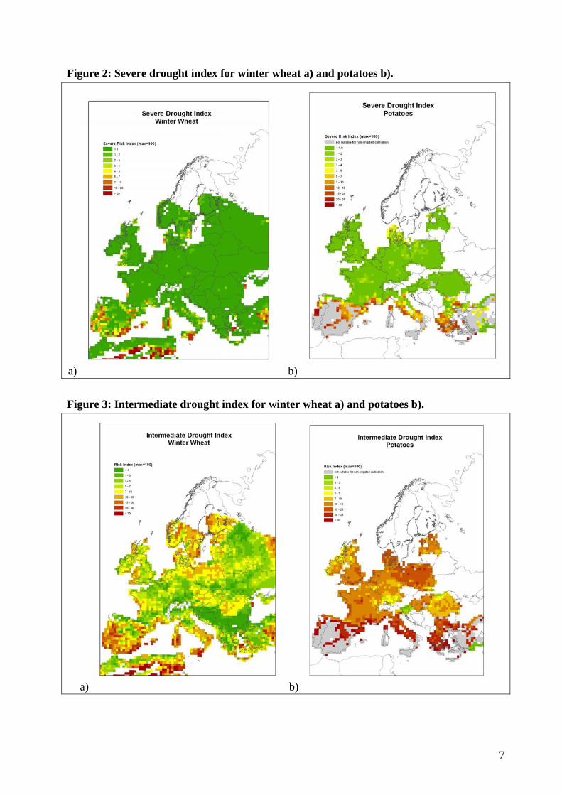
3.1 Drought The parameter selected to map the risk of drought is the relative soil moisture (RSM) estimated by CGMS using meteorological data interpolated in a 50-km grid focussing the estimation on the mean altitude of the part of the cell, in which agriculture is concentrated taken from the CORINE Land Cover data set, respectively Global Land Cover data set for areas outside the EU. RSM integrates the information on rainfall, soil water capacity and needs of the plant, taking into account the phenological calendar, the temperature and the global radiation. If CGMS estimates for a given crop a value 0 for the Relative Soil Moisture (RSM), this indicates a considerable water stress for that crop; if this happens during the development stages of growth, flowering or grain filling, this corresponds to a serious drought situation. The impact of a drought situation is not the same in all the development stages of the crop. We have made a first rough split before/after flowering starts. After the start of flowering (until short before maturity), a drought event is considered twice as serious as before flowering. When the grains (or other storage organs) have been filled and the plant is close to maturity, dry soil is not considered anymore a source of damage. Figure 2 reports the proportion of situations of serious drought for wheat in the period 1975-2006. Few areas have a significant risk of severe drought measured with this parameter. These areas are generally concentrated in southern Europe. Some spots also appear in central and Northern Europe, mainly in coastal areas; they might be due to computational artefacts in the meteorological data interpolation. Since the drought indices refer to non-irrigated agriculture, for some corps like sugar beets and potatoes threshold parameters have been introduced to exclude areas where these crops are cultivated only under irrigation (ref. to Figure 2b). A certain number of anomalies in these maps show that fine-tuning of parameters still needs to be improved. An alternative drought indicator has been defined considering an intermediate drought situation when the RSM <10% or the RSM < ½ min (40%, the long-term average RSM for that time of the year). This means for example that an RSM=15% in an area where the long term average is more than 30% will be considered an intermediate drought situation, but RSM=25% in an area where the long term average is more than 50% will not be considered drought at all. This indicator seems better modulated and show again most serious risks, but significant wheat growing areas appear to have drought problems in the area of northern Poland, east Germany, Baltic countries and Scandinavia, probably due to soils with relative low water retention potential (post-glacial soils, consisting of gravel, loose sands and loamy sands), see Figure 3 a) and b).

7

Figure 2: Severe drought index for winter wheat a) and potatoes b).

a) b) Figure 3: Intermediate drought index for winter wheat a) and potatoes b).

a) b)

8

3.2 Excessive rain We use meteorological data interpolated in the CGMS 50-km grid. Meteorological data are estimated for the mean altitude of the part of the cell, in which agriculture is concentrated taken from the CORINE Land Cover data set. For each cell c and each year t, we consider for each crop the rainfall in the decade of maturity r1,t,c, the decade before r0,t,c and the decade after r2,t,c.

ctctctct rrrr ,,2,,1,,0, ++= (1)

We consider that rainfall is harmful if it is higher than the local long-term average cr by more than 40 mm. In any case only mmr ct 80, > are considered potentially harmful. The following pages represent maps of an indicator of damage per year due to excessive rain at harvest time computed through:

( )⎩⎨⎧

+−+≤≤

=cct

cctctct rrelse

rrorrifyr

40,80max40800

,

,,, (2)

The long term risk indicator will be cry . This indicator still needs to be validated. it is based on agro-meteorologist expert knowledge and we use it at this stage to get a general view of the risk. The following figures depict the regional distribution of the risk index based on excessive rain events during harvest time.

a) b)

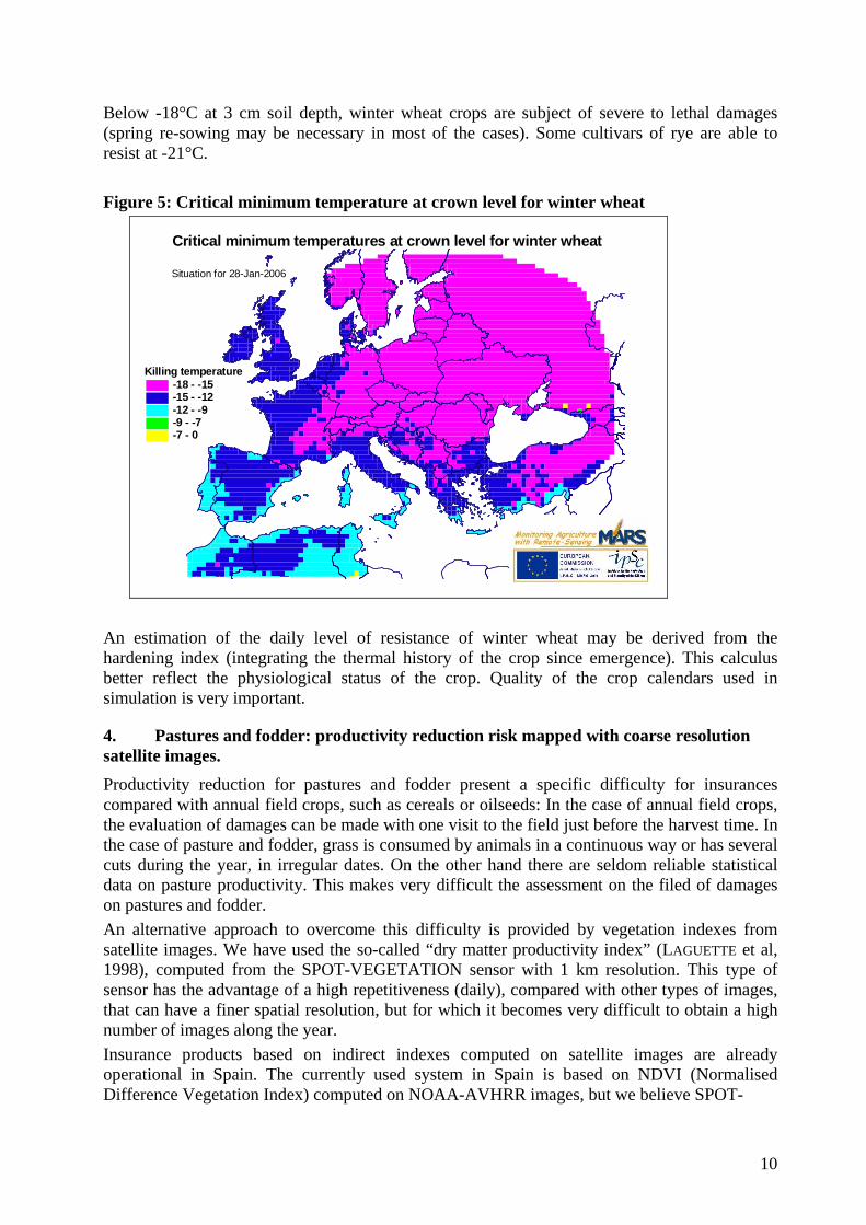
3.3 Frost Extreme cold in winter can make a substantial damage to crops. The level of damage obviously depends on the minimum temperatures, but should not be assessed by a straight mapping of minimum temperatures as reported by meteorological observatories (temperature of the air at 2 m above the ground). It requires some elaboration taking into account the recent thermal history (last days) and the protective effect of snow. A progressive lowering of temperatures is less harmful than an abrupt frost, because the plant has the time of protecting itself by a physiologic

9

process knows as hardening. The following maps (Figure 4) give an idea of the potential damage by low temperatures. A temperature of 0°C at 3 cm soil depth (crown level) doesn’t represent menace for the main winter crops but it implies the stop of the growth; temperatures between -6 and -9°C at 3 cm soil depth (crown level) may affect the unhardened sensitive winter cereals (like winter barley or durum wheat). Temperatures between -9 and -12°C at 3 cm soil depth may affect medium hardened sensible winter cereals (like winter barley or durum wheat) or unhardened winter wheat corps. Temperatures between -12 and -15°C at 3 cm soil depth may reduce drastically the plant population of sensible winter cereals (like winter barley or durum wheat) or even affect the medium hardened winter wheat corps. At temperatures between -15 and -18°C at 3 cm soil depth, winter crops like winter barley or durum wheat have very low chances of survival and serious damages for winter wheat are expected (depending on cultivar and hardening index). Figure 4: Maps with number of days per year with low temperatures at 3 cm soil depth.

10

Below -18°C at 3 cm soil depth, winter wheat crops are subject of severe to lethal damages (spring re-sowing may be necessary in most of the cases). Some cultivars of rye are able to resist at -21°C. Figure 5: Critical minimum temperature at crown level for winter wheat

Critical minimum temperatures at crown level for winter wheat

Situation for 28-Jan-2006

Killing temperature-18 - -15-15 - -12-12 - -9-9 - -7-7 - 0

An estimation of the daily level of resistance of winter wheat may be derived from the hardening index (integrating the thermal history of the crop since emergence). This calculus better reflect the physiological status of the crop. Quality of the crop calendars used in simulation is very important.

4. Pastures and fodder: productivity reduction risk mapped with coarse resolution satellite images.

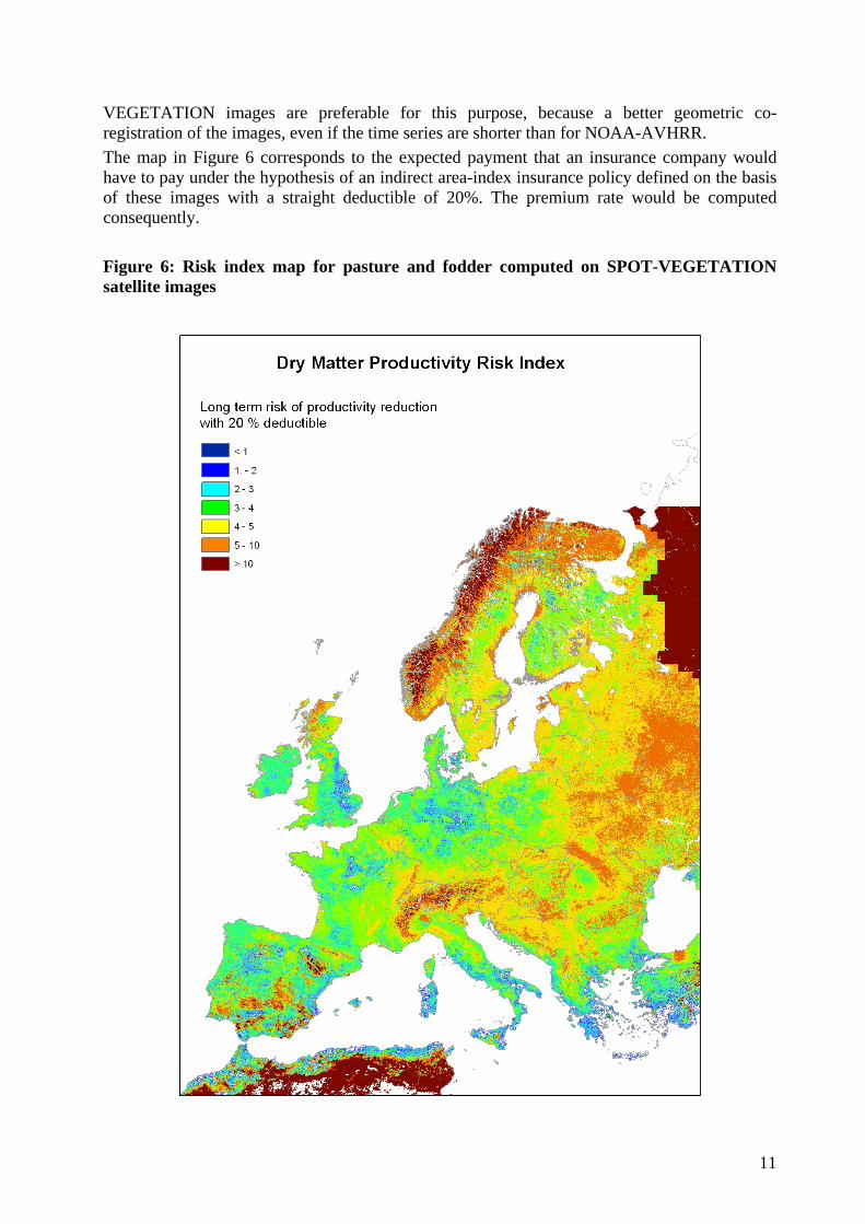
Productivity reduction for pastures and fodder present a specific difficulty for insurances compared with annual field crops, such as cereals or oilseeds: In the case of annual field crops, the evaluation of damages can be made with one visit to the field just before the harvest time. In the case of pasture and fodder, grass is consumed by animals in a continuous way or has several cuts during the year, in irregular dates. On the other hand there are seldom reliable statistical data on pasture productivity. This makes very difficult the assessment on the filed of damages on pastures and fodder. An alternative approach to overcome this difficulty is provided by vegetation indexes from satellite images. We have used the so-called “dry matter productivity index” (LAGUETTE et al, 1998), computed from the SPOT-VEGETATION sensor with 1 km resolution. This type of sensor has the advantage of a high repetitiveness (daily), compared with other types of images, that can have a finer spatial resolution, but for which it becomes very difficult to obtain a high number of images along the year. Insurance products based on indirect indexes computed on satellite images are already operational in Spain. The currently used system in Spain is based on NDVI (Normalised Difference Vegetation Index) computed on NOAA-AVHRR images, but we believe SPOT-

11

VEGETATION images are preferable for this purpose, because a better geometric co-registration of the images, even if the time series are shorter than for NOAA-AVHRR. The map in Figure 6 corresponds to the expected payment that an insurance company would have to pay under the hypothesis of an indirect area-index insurance policy defined on the basis of these images with a straight deductible of 20%. The premium rate would be computed consequently. Figure 6: Risk index map for pasture and fodder computed on SPOT-VEGETATION satellite images

12

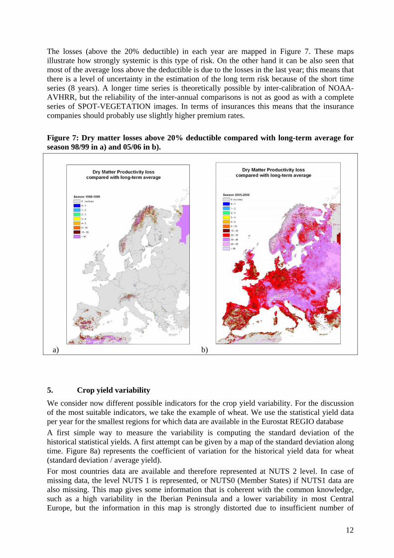
The losses (above the 20% deductible) in each year are mapped in Figure 7. These maps illustrate how strongly systemic is this type of risk. On the other hand it can be also seen that most of the average loss above the deductible is due to the losses in the last year; this means that there is a level of uncertainty in the estimation of the long term risk because of the short time series (8 years). A longer time series is theoretically possible by inter-calibration of NOAA-AVHRR, but the reliability of the inter-annual comparisons is not as good as with a complete series of SPOT-VEGETATION images. In terms of insurances this means that the insurance companies should probably use slightly higher premium rates. Figure 7: Dry matter losses above 20% deductible compared with long-term average for season 98/99 in a) and 05/06 in b).

a) b)

5. Crop yield variability We consider now different possible indicators for the crop yield variability. For the discussion of the most suitable indicators, we take the example of wheat. We use the statistical yield data per year for the smallest regions for which data are available in the Eurostat REGIO database A first simple way to measure the variability is computing the standard deviation of the historical statistical yields. A first attempt can be given by a map of the standard deviation along time. Figure 8a) represents the coefficient of variation for the historical yield data for wheat (standard deviation / average yield). For most countries data are available and therefore represented at NUTS 2 level. In case of missing data, the level NUTS 1 is represented, or NUTS0 (Member States) if NUTS1 data are also missing. This map gives some information that is coherent with the common knowledge, such as a high variability in the Iberian Peninsula and a lower variability in most Central Europe, but the information in this map is strongly distorted due to insufficient number of

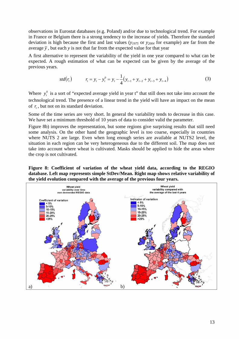
13

observations in Eurostat databases (e.g. Poland) and/or due to technological trend. For example in France or Belgium there is a strong tendency to the increase of yields. Therefore the standard deviation is high because the first and last values (y1975 or y2004 for example) are far from the average y , but each y is not that far from the expected value for that year A first alternative to represent the variability of the yield in one year compared to what can be expected. A rough estimation of what can be expected can be given by the average of the previous years.

( ) ( )43210

41

−−−− +++−=−= ttttttttt yyyyyyyrrstd (3)

Where 0ty is a sort of “expected average yield in year t” that still does not take into account the

technological trend. The presence of a linear trend in the yield will have an impact on the mean of tr , but not on its standard deviation.

Some of the time series are very short. In general the variability tends to decrease in this case. We have set a minimum threshold of 10 years of data to consider valid the parameter. Figure 8b) improves the representation, but some regions give surprising results that still need some analysis. On the other hand the geographic level is too coarse, especially in countries where NUTS 2 are large. Even when long enough series are available at NUTS2 level, the situation in each region can be very heterogeneous due to the different soil. The map does not take into account where wheat is cultivated. Masks should be applied to hide the areas where the crop is not cultivated. Figure 8: Coefficient of variation of the wheat yield data, according to the REGIO database. Left map represents simple StDev/Mean. Right map shows relative variability of the yield evolution compared with the average of the previous four years.

a) b)

14

5.1 Applying a deductible When a yield reduction indicator ri from statistical data has been identified as acceptable, we can build an indicator, instead of std(rt) , that behaves close to the insurance cost assuming a d=20% deductible:

If drsdr

sdr

ttt

tt

−=>=< 0

(4)

ts∑ would be the expectation of payment that an insurance company would pay to a

hypothetical farm that would have the average regional yield if this hypothetical farm has an insurance on the expected yield with a deductible d (10%, or 20% for example).

5.2 Comparing with a yield trend A better option is comparing the regional yield of each year with an adjusted trend. In order to estimate a trend we have made a quadratic stepwise regression of the time series in each region. We assume that the trend is growing or constant and its slope is constant or decreasing. We obtain this with the following rules:

• If none of the time terms is significant or the regression-adjusted trend is decreasing, the average yield is accepted as trend.

• If the linear term is significant and the quadratic is not significant or has a positive sign, we take a linear trend.

• If the quadratic trend goes down before the end of the series, we keep it constant after the maximum value.

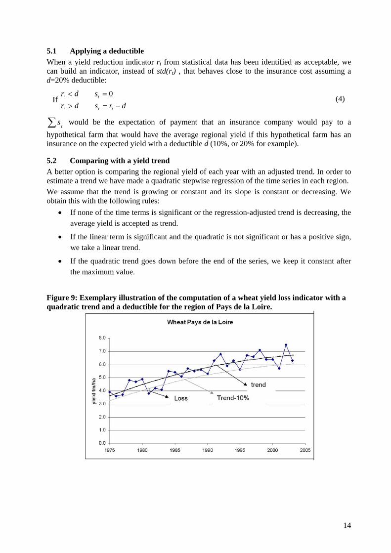
Figure 9: Exemplary illustration of the computation of a wheat yield loss indicator with a quadratic trend and a deductible for the region of Pays de la Loire.

15

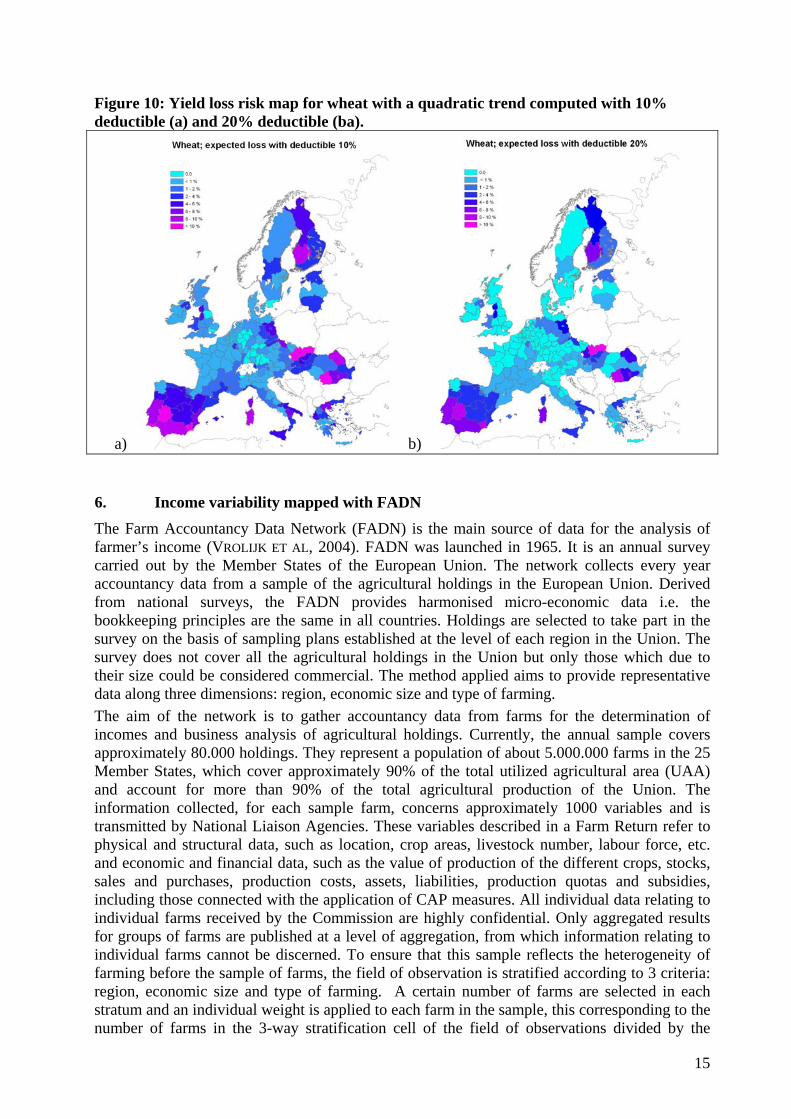
Figure 10: Yield loss risk map for wheat with a quadratic trend computed with 10% deductible (a) and 20% deductible (ba).

a) b)

6. Income variability mapped with FADN The Farm Accountancy Data Network (FADN) is the main source of data for the analysis of farmer’s income (VROLIJK ET AL, 2004). FADN was launched in 1965. It is an annual survey carried out by the Member States of the European Union. The network collects every year accountancy data from a sample of the agricultural holdings in the European Union. Derived from national surveys, the FADN provides harmonised micro-economic data i.e. the bookkeeping principles are the same in all countries. Holdings are selected to take part in the survey on the basis of sampling plans established at the level of each region in the Union. The survey does not cover all the agricultural holdings in the Union but only those which due to their size could be considered commercial. The method applied aims to provide representative data along three dimensions: region, economic size and type of farming. The aim of the network is to gather accountancy data from farms for the determination of incomes and business analysis of agricultural holdings. Currently, the annual sample covers approximately 80.000 holdings. They represent a population of about 5.000.000 farms in the 25 Member States, which cover approximately 90% of the total utilized agricultural area (UAA) and account for more than 90% of the total agricultural production of the Union. The information collected, for each sample farm, concerns approximately 1000 variables and is transmitted by National Liaison Agencies. These variables described in a Farm Return refer to physical and structural data, such as location, crop areas, livestock number, labour force, etc. and economic and financial data, such as the value of production of the different crops, stocks, sales and purchases, production costs, assets, liabilities, production quotas and subsidies, including those connected with the application of CAP measures. All individual data relating to individual farms received by the Commission are highly confidential. Only aggregated results for groups of farms are published at a level of aggregation, from which information relating to individual farms cannot be discerned. To ensure that this sample reflects the heterogeneity of farming before the sample of farms, the field of observation is stratified according to 3 criteria: region, economic size and type of farming. A certain number of farms are selected in each stratum and an individual weight is applied to each farm in the sample, this corresponding to the number of farms in the 3-way stratification cell of the field of observations divided by the

16

number of farms in the corresponding cell in the sample. This weighting system is used in the calculation of standard results and generally also for the estimations in specific studies. The standard results are a set of statistics, calculated from the Farm Returns, which are periodically produced and published by the Commission. They describe in considerable detail the economic situation of farmers by different groups. The FADN survey covers the entire range of agricultural activities on farms. It also collects data on non-agricultural farming activities (such as tourism and forestry). FADN provides in fact a unique source of data to analyse the income of farmers making the difference between different types of farms, size of the holding and regions. Figure 11 gives an exemplary overview of spatial distribution of income reduction risk for different farm types in the EU. The data are shown for the so-called “FADN regions” (in general NUTS0, NUTS 1 or NUTS2 regions, depending on the country). They have been calculated considering the time series of average income/AWU (Annual Work Unit) for each major farm type (or farm size category). A trend is estimated on the basis of this time series. Any income average below the trend by more than a deductible of 10% is considered a significant loss. This approach has several limitations and needs a more in-depth analysis. The main limitation is that considering the behaviour of the “average farm” for each class and region smoothes down a lot of the irregularities in farm income. This leads to an underestimation of the reduction risk that is in part compensated by choosing a low deductible level (10%). Figure 11: Risk index for income reduction: field crop specialists and grazing livestock.

FADN data allow to a certain extent a simulation of what would have happened without insurances; in particular the costs of insurances are collected for each farm of the sample. Unfortunately the compensations received by farmers in case of crisis are insufficiently detailed for a proper analysis. Therefore additional information collected during a survey on agricultural insurances in the EU was used for calculating the amount of insurance compensations (GALLEGO ET AL., 2006). The data for different countries do not correspond to the same period of time, and there is a large variation of compensations from one year to another, but we can say that the average compensation that farmers obtain from insurers is around 1000 M€/year. In order to know which part of the problem these payments reduce, we have to quantify the income reduction risk. Quantification of the income reduction risk necessarily involves some subjectivity. We have chosen an indicator computed on an approach that is consistent with the maps, i.e. based on the time series of average income/AWU for each major farm type (or farm size category), considering a significant loss the one corresponding to an income below the trend by more than a 10% deductible.

17

The total reduction is around 3000-3500 M€/year and would be around 1000 M€/year higher without agricultural insurances. This means that agricultural insurances mitigate significant farm reduction income by around 22-25%.

References BEEK, E.G., 1991 . Spatial interpolation of daily meteorological data. Theoretical evaluation of

available techniques. Report 53.1, DLO Winand Staring Centre, Wageningen, The Netherlands , pp 43.

DE KONING G. H. J., JANSEN M. J. W..,BOONS-PRINS E. R., VAN DIEPEN C. A., PENNING DE VRIES F. W. T., 1993, Crop growth simulation and statistical validation for regional yield forecasting across the European Community, Simulations Reports CABO-TT, no 31, Wageningen Agricultural University, CABO-DLO, JRC.

GALLEGO J. F., BIELZA M., CONTE C., DITTMANN CH., STROBLMAIR J., 2006, Agricultural Insurance Schemes, Administrative Arrangement n° AGRI-2005-0321....between DG Agriculture (DG AGRI) and DG Joint Research Centre (JRC), Ispra, Italy.

GENOVESE G., 1994, Yield forecasting and operational approaches using remote sensing: Overview of approaches and operational applications in the E.U., Proceedings of the seminar on crop forecasting methods, pp 79-86. Villefranche 24-27 October, Office for Publications of the EC. ISBN 92-827-9451-2.

GENOVESE G., 1998. The methodology and the results of the MARS bulletin: an integrated crop production assessment and forecast in bulletin. In Agrometeorological applications for regional crop monitoring and production assessment, Office for Publications of the EC. Luxembourg. EUR 17735 EN pp. 67-120.

GOOT, E. VAN DER, 1998. Spatial interpolation of daily meteorological data for the Crop Growth Monitoring System (CGMS). In: M. Bindi, B. Gozzini (eds). Proceedings of seminar on data spatial distribution in meteorology and climatology, 28 September - 3 October 1997 , Volterra , Italy . EUR 18472 EN, Office for Official Publications of the EU, Luxembourg , p 141-153.

LAGUETTE, S., VIDAL, A. & VOSSEN, P., (1998), Using NOAA-AVHRR data to forecast wheat yields at a European scale, In "Agrometeorological applications for regional crop growth monitoring and production assessment", pp. 131-146, EU JRC, eds. D.Rijks, J.M. Terres & P.Vossen;

MONTEITH, J. L. 1985. Evaporation from land surfaces: progress in analysis and prediction since 1948. pp. 4-12. In Advances in Evapotranspiration, Proceedings of the ASAE Conference on Evapotranspiration, Chicago, Ill. ASAE, St. Joseph, Michigan.

RODRIGUEZ, D., VAN OIJEN, M., SCHAPENDONK, A.H.M.C., 1999, LINGRA-CC: A sink-source model to simulate the impact of climate change and management on grassland productivity, New Phytologist, Volume 144, Issue 2, November 1999, Pages 359-368

SCHAPENDONK, A.H.C.M., STOL, W., VAN KRAALINGEN, D.W.G., BOUMAN, B.A.M. (1998): LINGRA, a sink/source model to simulate grassland productivity in Europe European Journal of Agronomy 9 (2-3), pp. 87-100

SUPIT, I. , 1994. Global radiation. EUR 15745 EN, Office for Official Publications of the EU, Luxembourg , pp 194.

SUPIT, I., HOOIJER, A.A., VAN DIEPEN, C.A., 1994. System description of the WOFOST 6.0 crop simulation model implemented in CGMS. EUR Publication N° 15956 EN of the Office for Official Publications of the European Communities. Luxembourg,. 168 pp.

18

VAN DIEPEN C.A., WOLF C.A., VAN KEULEN H., RAPPOLDT C., 1989. WOFOST: a simulation model of crop production. Soils use and Management. vol 5, n° 1, pp 16-24.

VOET, P. VAN DER., DIEPEN, C.A. VAN, OUDE VOSHAAR, J., 1994. Spatial interpolation of daily meteorological data. A knowledge-based procedure for the regions of the European Communities. Report 53.3, DLO Winand Staring Centre, Wageningen, The Netherlands , pp 105.

VROLIJK, H.C.J., MEIER, B., KLEINHANßE, W., POPPE, K.J., 2004, FADN: Buttress for farm policy or a resource for economic analysis? EuroChoices 3 (3), pp. 32-37.