Manual KNIME Image Processing :: First steps This manual aims to provide first insights in KNIME Image Processing. The image processing workflow ‘Count nuclei’ is described in detail and can be downloaded from the workflow repository. The corresponding example raw data is available as well. Please note, that the three example workflows

1) Count nuclei 2) Cytoplasm intensity 3) Spots finder

are based on each other, i.e. the complexity increases from workflow 1) to workflow 3). If you would like to use the ‘Spots finder’ workflow we recommend to start with ‘Count nuclei’! After the installation of the KNIME –Desktop including the additional plugins (cp. Installation of the KNIME –Desktop) you can load the example workflow ‘Count nuclei’: GoTo [ File ] → [ Import KNIME workflow… ] → Select archive file: and import the ‘CountNuclei.zip’ example workflow. The workflow now appears in the KNIME Explorer on the left hand side of the KNIME –Desktop. Launch the workflow (double-click). Overview: The workflow loads five image raw data files (.tif files of nucleus image raw data from an Olympus microscope), segments the objects and performs a basic quality control step in order to identify the nuclei. The workflow itself consists of three parts:

o STEP 1: Process Images… Explains the basic image processing functionality without any additional (table) processing

o STEP 2: Apply “table processing” and run basic statistics… Provides in addition to STEP 1 some basic table transformations for extracting image meta data and runs basic statistics in order to get the number of nuclei

o STEP 3: Process image by image using loops… Provides in addition to STEP 1 & STEP 2 loop processing of single images

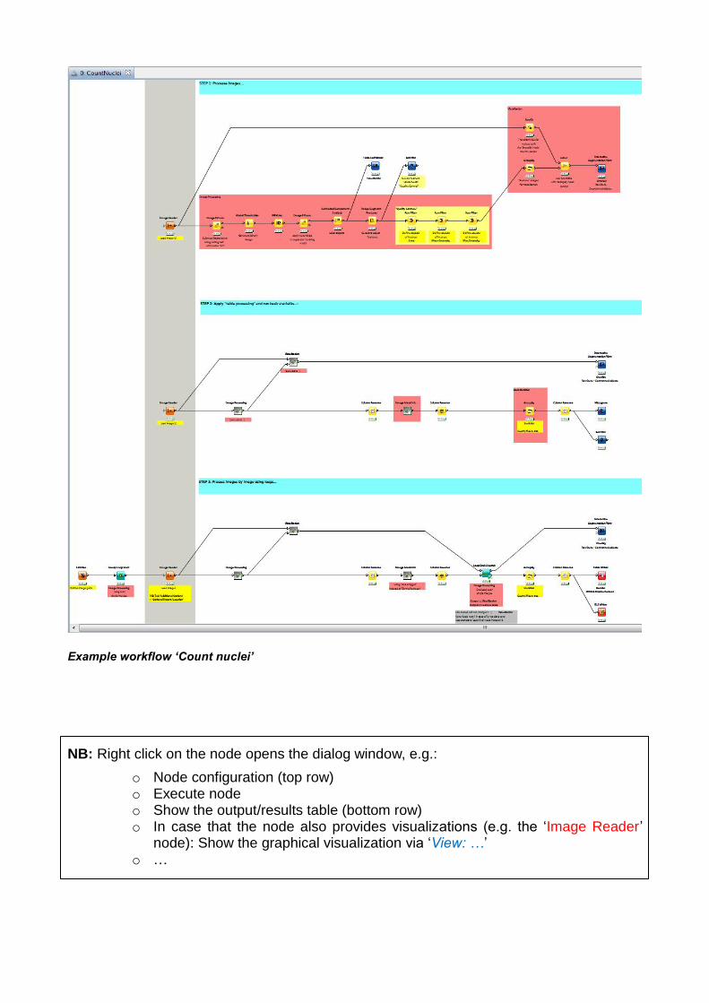
Example workflow ‘Count nuclei’

NB: Right click on the node opens the dialog window, e.g.:

o Node configuration (top row) o Execute node o Show the output/results table (bottom row) o In case that the node also provides visualizations (e.g. the ‘Image Reader’

node): Show the graphical visualization via ‘View: …’ o …

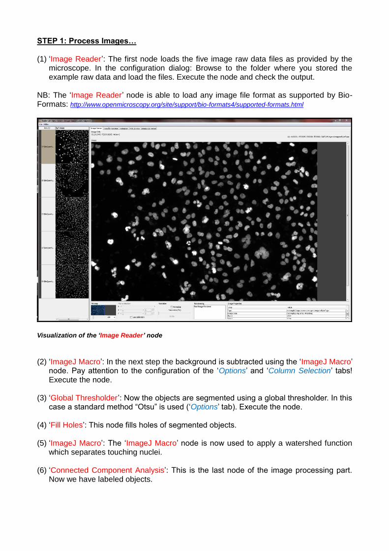
STEP 1: Process Images… (1) ‘Image Reader’: The first node loads the five image raw data files as provided by the

microscope. In the configuration dialog: Browse to the folder where you stored the example raw data and load the files. Execute the node and check the output.

NB: The ‘Image Reader’ node is able to load any image file format as supported by Bio-Formats: http://www.openmicroscopy.org/site/support/bio-formats4/supported-formats.html

Visualization of the ‘Image Reader’ node

(2) ‘ImageJ Macro’: In the next step the background is subtracted using the ‘ImageJ Macro’

node. Pay attention to the configuration of the ‘Options’ and ‘Column Selection’ tabs! Execute the node.

(3) ‘Global Thresholder’: Now the objects are segmented using a global thresholder. In this

case a standard method “Otsu” is used (‘Options’ tab). Execute the node. (4) ‘Fill Holes’: This node fills holes of segmented objects.

(5) ‘ImageJ Macro’: The ‘ImageJ Macro’ node is now used to apply a watershed function

which separates touching nuclei.

(6) ‘Connected Component Analysis’: This is the last node of the image processing part. Now we have labeled objects.

Visualization of the ‘Global Thresholder’ node

Visualization of the ‘Connected Component Analysis’ node

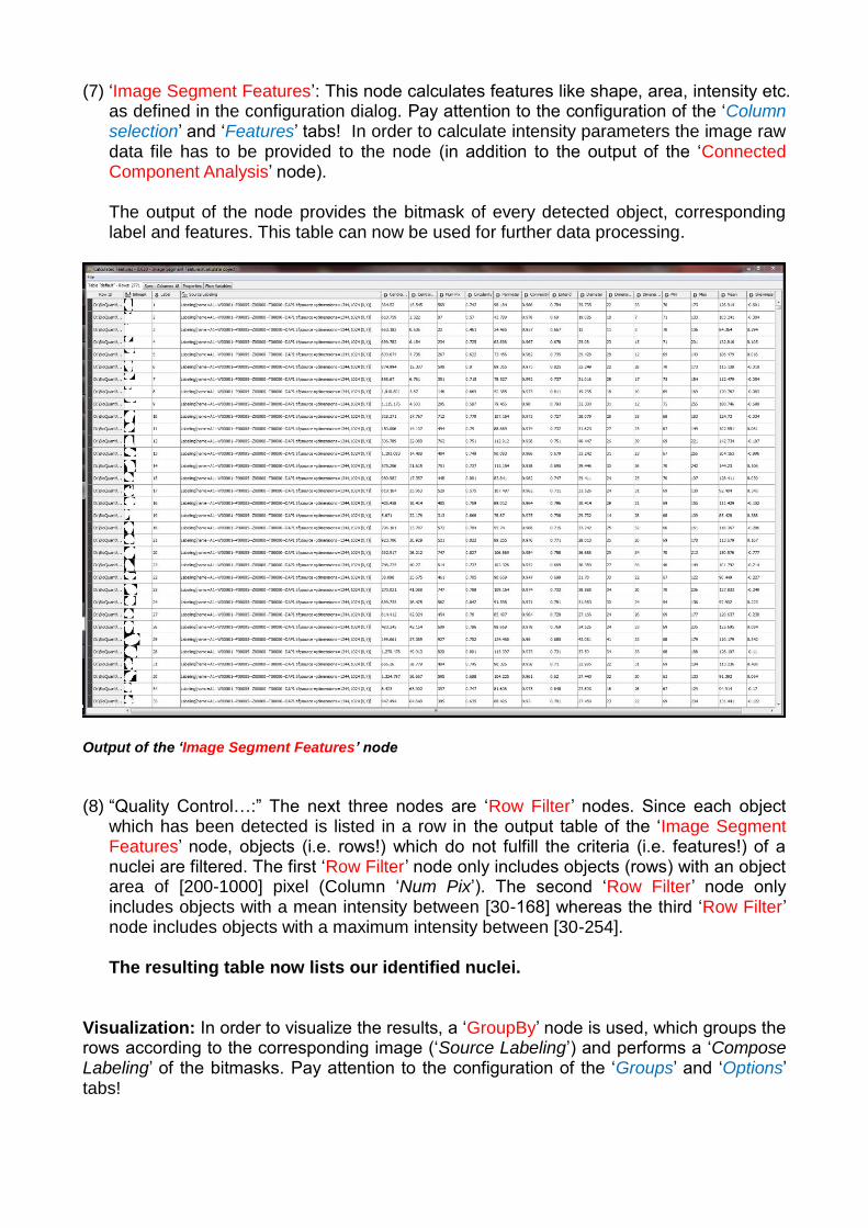
(7) ‘Image Segment Features’: This node calculates features like shape, area, intensity etc. as defined in the configuration dialog. Pay attention to the configuration of the ‘Column selection’ and ‘Features’ tabs! In order to calculate intensity parameters the image raw data file has to be provided to the node (in addition to the output of the ‘Connected Component Analysis’ node).

The output of the node provides the bitmask of every detected object, corresponding label and features. This table can now be used for further data processing.

Output of the ‘Image Segment Features’ node

(8) “Quality Control…:” The next three nodes are ‘Row Filter’ nodes. Since each object

which has been detected is listed in a row in the output table of the ‘Image Segment Features’ node, objects (i.e. rows!) which do not fulfill the criteria (i.e. features!) of a nuclei are filtered. The first ‘Row Filter’ node only includes objects (rows) with an object area of [200-1000] pixel (Column ‘Num Pix’). The second ‘Row Filter’ node only includes objects with a mean intensity between [30-168] whereas the third ‘Row Filter’ node includes objects with a maximum intensity between [30-254]. The resulting table now lists our identified nuclei.

Visualization: In order to visualize the results, a ‘GroupBy’ node is used, which groups the rows according to the corresponding image (‘Source Labeling’) and performs a ‘Compose Labeling’ of the bitmasks. Pay attention to the configuration of the ‘Groups’ and ‘Options’ tabs!

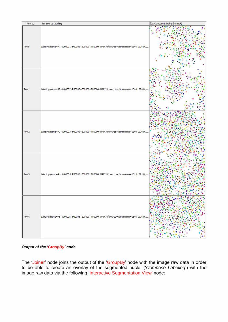
Output of the ‘GroupBy’ node

The ‘Joiner’ node joins the output of the ‘GroupBy’ node with the image raw data in order to be able to create an overlay of the segmented nuclei (‘Compose Labeling’) with the image raw data via the following ‘Interactive Segmentation View’ node:

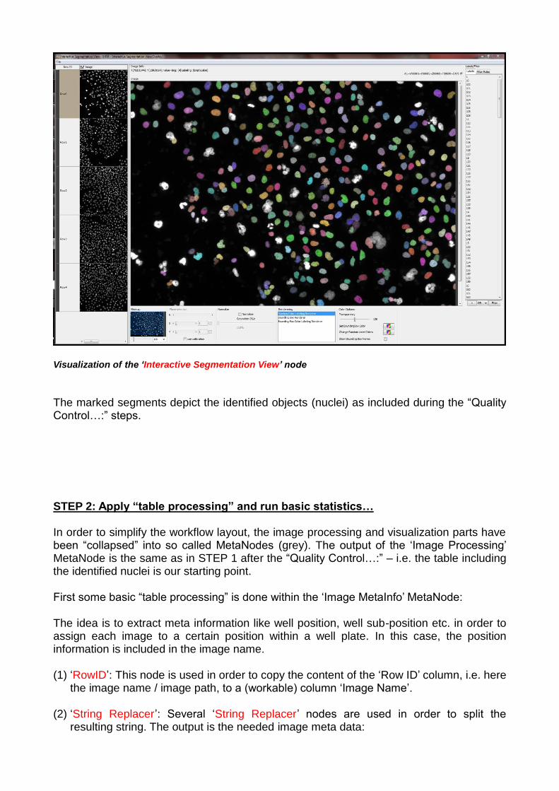
Visualization of the ‘Interactive Segmentation View’ node

The marked segments depict the identified objects (nuclei) as included during the “Quality Control…:” steps. STEP 2: Apply “table processing” and run basic statistics… In order to simplify the workflow layout, the image processing and visualization parts have been “collapsed” into so called MetaNodes (grey). The output of the ‘Image Processing’ MetaNode is the same as in STEP 1 after the “Quality Control…:” – i.e. the table including the identified nuclei is our starting point. First some basic “table processing” is done within the ‘Image MetaInfo’ MetaNode: The idea is to extract meta information like well position, well sub-position etc. in order to assign each image to a certain position within a well plate. In this case, the position information is included in the image name. (1) ‘RowID’: This node is used in order to copy the content of the ‘Row ID’ column, i.e. here

the image name / image path, to a (workable) column ‘Image Name’.

(2) ‘String Replacer’: Several ‘String Replacer’ nodes are used in order to split the resulting string. The output is the needed image meta data:

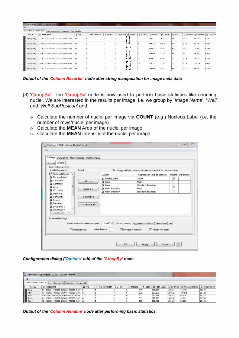
Output of the ‘Column Resorter’ node after string manipulation for image meta data

(3) ‘GroupBy’: The ‘GroupBy’ node is now used to perform basic statistics like counting

nuclei. We are interested in the results per image, i.e. we group by ‘Image Name’, ‘Well’ and ‘Well SubPosition’ and

o Calculate the number of nuclei per image via COUNT (e.g.) Nucleus Label (i.e. the

number of rows/nuclei per image) o Calculate the MEAN Area of the nuclei per image o Calculate the MEAN Intensity of the nuclei per image

Configuration dialog (‘Options’ tab) of the ‘GroupBy’ node

Output of the ‘Column Rename’ node after performing basic statistics

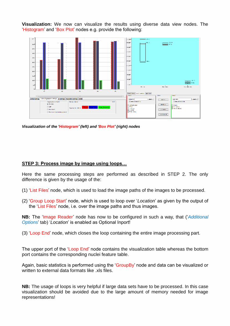
Visualization: We now can visualize the results using diverse data view nodes. The ‘Histogram’ and ‘Box Plot’ nodes e.g. provide the following:

Visualization of the ‘Histogram’ (left) and ‘Box Plot’ (right) nodes

STEP 3: Process image by image using loops… Here the same processing steps are performed as described in STEP 2. The only difference is given by the usage of the: (1) ‘List Files’ node, which is used to load the image paths of the images to be processed. (2) ‘Group Loop Start’ node, which is used to loop over ‘Location’ as given by the output of

the ‘List Files’ node, i.e. over the image paths and thus images.

NB: The ‘Image Reader’ node has now to be configured in such a way, that (‘Additional Options’ tab) ‘Location’ is enabled as Optional Inport! (3) ‘Loop End’ node, which closes the loop containing the entire image processing part. The upper port of the ‘Loop End’ node contains the visualization table whereas the bottom port contains the corresponding nuclei feature table. Again, basic statistics is performed using the ‘GroupBy’ node and data can be visualized or written to external data formats like .xls files. NB: The usage of loops is very helpful if large data sets have to be processed. In this case visualization should be avoided due to the large amount of memory needed for image representations!