MANAGEMENT OF QUALITY AND

QUALITY CONTROL

In the world of science and technology, it has become absolutely necessary for a

businessman to keep a continuous watch over the quality of the goods produced.

Having once bought the product, if the consumers feel satisfied with regard to its

quality, price etc., a kind of goodwill for the product is developed which helps to

increase the sales. However, if the consumers are not happy with the quality of the

product and their complaints are not given proper attention, it shell be impossible for

the manufacturer to continue in the market.

It is important to distinguish between the unsystematic inspection and supervision

which often goes under the name of "quality control" and statistical quality control. The

quality control does not say when or how samples should be taken or how large they

should be also it does not have the advantages that go with graphic presentation and a

clear objective standard is not enforced for "take action" or "skip it". The statistical

quality control chart makes use of well through-out, tested rules and avoids the

indecision, inconsistency and arbitrariness of haphazard quality control.

The term 'quality' in statistical quality control is usually related to some measurement

made on the items produced a good quality item having one which confirms to

standards specified for measurement. Quality does not always imply the highest,

standards of manufacturer, for the standard required is often deliberately below the

highest possible. It is almost always consistency in quality standards which represents

PRODUCTION AND OPERATIONS MANAGEMENT

the most desirable situation rather than the absolute standard which is maintained. The

need for quality control arises because of the fact that even after the quality standards

have been specified some variation in quality is unavoidable.

Quality control plays a very important role in the process of manufacturing. The

problem of production adaptation to customer requirement has now become

increasingly serious. Management uses a wide range of tools in manufacturing goods

that involve good workmanship, design materials and other characteristics. These

quality products encourage customers even to pay premium prices. This also leads to

customer satisfaction. If poor quality of goods are supplied to customers, they refuse to

accept and instead go in for substitute products. This results in reduced sales. Hence

the need for quality control.

The importance of quality control can be highlighted under the following points.

It increases the profit earning capacity of the business.

It enables the industry to complete successfully.

It reduces cost of production.

It reduces operating losses by keeping scraps and wastes to a minimum.

It improves the product design.

It reduces bottleneck product line.

It improves morale of the employees.

It enhances satisfaction of customers.

It increases reputation of the industry.

To fully understand the modern quality control movement, we need to look at the

philosophies of notable individuals who have shaped the evolution of Total Quality

Management. Their philosophies and teachings have contributed to our knowledge

and understanding of quality today.

Walter A. Shewhart was a statistician at Bell Labs during the 1920s and 1930s.

Shewhart studied randomness and recognized that variability existed in all

manufacturing processes. He developed quality control charts that are used to identify

whether the variability in the process is random or due to an assignable cause, such as

poor workers or mis-calibrated machinery. He stressed that eliminating variability

improves quality. His work created the foundation for today’s statistical process

control, and he is often referred to as the “grandfather of quality control.”

MANAGING FOR QUALITY CHAPTER - 9

W. Edwards Deming is often referred to as the “father of quality control.” He was a

statistics professor at New York University in the 1940s. After World War II, he

assisted many Japanese companies in improving quality. The Japanese regarded him

so highly that in 1951 they established the Deming Prize, an annual award given to

firms that demonstrate outstanding quality. It was almost 30 years before American

businesses began adopting Deming’s philosophy. Time line showing the differences

between old and new concepts of quality

Joseph M. Juran, like Deming, taught Japanese manufacturers how to improve the

quality of their goods, and he, too, can be regarded as a major force in Japan's success

in quality. Juran viewed quality as fitness-for-use. He also believed that roughly 80

percent of quality defects are management controllable; thus, management has the

responsibility to correct this deficiency. He described quality management in terms of

a trilogy consisting of quality planning, quality control, and quality improvement.

According to Juran, quality planning is necessary to establish processes that

are capable of meeting quality standards; quality control is necessary in order to know

when corrective action is needed; and quality improvement will help to find better

ways of doing things. A key element of Juran's philosophy is the commitment of

management to continual improvement.

Juran is credited as one of the first to measure the cost of quality, and he demonstrated

the potential for increased profits that would result if the costs of poor quality could be

reduced.

PRODUCTION AND OPERATIONS MANAGEMENT

Armand Feigenbaum was instrumental in advancing the “cost of nonconformance”

approach as a reason for management to commit to quality. He recognized that quality

was not simply a collection of tools and techniques, but a “total field.” According to

Feigenbaum, it is the customer who defines quality.

Philip B. Crosby developed the concept of zero defects and popularized the phrase

“Do it right the first time.” He stressed prevention, and he argued against the idea that

“there will always be some level of defectives.” In 1979, his book Quality is Free was

published. The quality-is-free concept is that the costs of poor quality are much greater

than traditionally defined. According to Crosby, these costs are so great that rather

than viewing quality efforts as costs, organizations should view them as a way to

reduce costs, because the improvements generated by quality efforts will more than

pay for themselves.

Crosby believes that any level of defects is too high and he maintains that achieving

quality can be relatively easy. His book Quality without Tears: The Art of Hassle-Free

Management was published in 1984.

Kaoru Ishikawa. The late Japanese expert on quality was strongly influenced by both

Deming and Juran, although he made significant contributions of his own to quality

management. Among his key contributions were the development of the cause-and-

effect diagram (also known as a fishbone diagram) for problem solving and the

implementation of quality circles, which involve workers in quality improvement. He

was the first quality expert to call attention to the internal customer—the next person in

the process, the next operation, within the organization.

Genichi Taguchi is best known for the Taguchi loss function, which involves a formula

for determining the cost of poor quality. The idea is that the deviation of a part from a

standard causes a loss, and the combined effect of deviations of all parts from their

standards can be large, even though each individual deviation is small.

Taiichi Ohno and Shigeo Shingo both developed the philosophy and methods

of kaizen, a Japanese term for continuous improvement at Toyota. Continuous

improvement is one of the hallmarks of successful quality management.

Quality awards have been established to generate improvement in quality. The

Malcolm Baldrige Award, the European Quality Award, and the Deming Prize are

well-known awards given annually to recognize firms that have integrated quality

management in their operations.

MANAGING FOR QUALITY CHAPTER - 9

The Malcolm Baldridge national Quality Award

The Malcolm Baldridge National Quality Award was established in 1987, when Congress

passed the Malcolm Baldridge National Quality Improvement Act. The award is named

after the former Secretary of Commerce, Malcolm Baldridge, and is intended to reward

and stimulate quality initiatives. It is designed to recognize companies that establish and

demonstrate high quality standards. The purpose of the award competition is to

stimulate efforts to improve quality, to recognize quality achievements, and to publicize

successful programs. The award is given to no more than two companies in each of three

categories: manufacturing, service, and small business. Past winners include Motorola

Corporation, Xerox, FedEx, 3M, IBM, and the Ritz-Carlton.

To compete for the Baldrige Award, companies must submit a lengthy application,

which is followed by an initial screening. Companies that pass this screening move to

the next step, in which they undergo a rigorous evaluation process conducted by

certified Baldrige examiners. The examiners conduct site visits and examine numerous

company documents. They base their evaluation on seven categories.

The first category is leadership. Examiners consider commitment by top

management,their effort to create an organizational climate devoted to quality, and

their active involvement in promoting quality. They also consider the firm’s orientation

toward meeting customer needs and desires, as well as those of the community and

society as a whole.

The second category is strategic planning. The examiners look for a strategic plan that

has high quality goals and specific methods for implementation.

The next category, customer and market focus, addresses how the company collects

market and customer information. Successful companies should use a variety of tools

toward this end, such as market surveys and focus groups. The company then needs to

demonstrate how it acts on this information.

The fourth category is information and analysis. Examiners evaluate how the company

obtains data and how it acts on the information. The company needs to demonstrate

how the information is shared within the company as well as with other parties, such

as suppliers and customers.

The fifth and sixth categories deal with management of human resources and

management of processes, respectively. These two categories together address the

issues of people and process. Human resource focus addresses issues of employee

involvement.This entails continuous improvement programs, employee training, and

functioning of teams. Employee involvement is considered a critical element of quality.

Similarly, process management involves documentation of processes, use of tools for

quality improvement such as statistical process control, and the degree of process

integration within the organization.

PRODUCTION AND OPERATIONS MANAGEMENT

The last Baldrige category receives the highest points and deals with business results.

Numerous measures of performance are considered, from percentage of defective

items to financial and marketing measures. Companies need to demonstrate

progressive improvement in these measures over time, not only a one-time

improvement.

The Baldrige criteria have evolved from simple award criteria to a general framework

for quality evaluation. Many companies use these criteria to evaluate their own

performance and set quality targets even if they are not planning to formally compete

for the award.

Categories Points

1. Leadership 120

2. Strategic planning 85

3. Customer and Market Focus 85

4. Information and Analysis 90

5. Human Resource focus 85

6. Process Management 85

7. Business Results 450

Total 1000

Fig; Baldrige criteria for performance excellence framework: A systems perspective

MANAGING FOR QUALITY CHAPTER - 9

The European Quality Awards

This award is Europe's most prestigious award for organizational excellence. The

European Quality Award sits at the top of regional and national quality awards and

applicants have often won one or more of those awards prior to applying for the

European Quality Award.

The Deming prize

The Deming Prize is a Japanese award given to companies to recognize their efforts in

quality improvement. The award is named after W. Edwards Deming, who visited

Japan after World War II upon the request of Japanese industrial leaders and

engineers. While there, he gave a series of lectures on quality. The Japanese considered

him such an important quality guru that they named the quality award after him.

The award has been given by the Union of Japanese Scientists and Engineers (JUSE)

since 1951. Competition for the Deming Prize was opened to foreign companies in

1984. In 1989, Florida Power & Light was the first U.S. company to receive the award.

The major focus of the judging is on statistical quality control, making it much

narrower in scope than the Baldrige Award, which focuses more on customer

satisfaction. Companies that win the Deming Prize tend to have quality programs that

are detailed and well-communicated throughout the company. Their quality

improvement programs also reflect the involvement of senior management and

employees, customer satisfaction, and training.

Japan also has an additional award, the Japan Prize, fashioned roughly after the

Baldrige Award.

Quality Certification

The International Organization for Standardization (ISO) promotes worldwide

standards for the improvement of quality, productivity, and operating efficiency

through a series of standards and guidelines. Used by industrial and business

organizations, regulatory agencies, governments, and trade organizations, the

standards have important economic and social benefits. Not only are they

tremendously important for designers, manufacturers, suppliers, service providers,

and customers, but the standards make a tremendous contribution to society in

general: They increase the levels of quality and reliability, productivity, and safety,

while making products and services affordable. The standards help facilitate

international trade. They provide governments with a base for health, safety, and

environmental legislation. And they aid in transferring technology to developing

countries.

There are two most widely accepted and used standards of ISO – ISO 9000 and ISO

14000. ISO 9001 deals with the quality management system while ISO 14000 concerns

PRODUCTION AND OPERATIONS MANAGEMENT

what an organization does to minimize harmful effects to the environment caused by

its operations. The standards are generic: no matter what the organization's business. If

an organization wants to establish a quality management system or an environmental

management system, the system must have the essential elements contained in ISO

9000 or in ISO 14000. The ISO 9000 standards are critical for companies doing business

internationally. They must go through a process that involves documenting quality

procedures and on-site assessment. With certification comes registration in an ISO

directory that companies seeking suppliers can refer to for a list of certified companies.

ISO 9000 Series

ISO 9000 is a group of generic standards which specify what should be in a company’s

quality system whatever the product or service. Set up by the international

organization for standardization (ISO) in Geneva, ISO 9000 standard was started in

1989 to provide a universal framework for quality assurance among its 12 member nations.

ISO 9000 standards do not refer to the technical specification of products but to the

systems producing them, assuring that products consistently have the quality that buyers expect. The standard consist of five parts.

ISO 9000

It is a quality standard that sets out the methods by which a management system

incorporating all the activities associated with quality can be implemented in an

organization to ensure that all the special performance requirements and the needs of

the customer are finally met. The system applies to the quality management systems a company uses not its products.

ISO 9001

It provides the model for an organization which is involved in the management of

design as well as in producing the product or service. Thus, in service organizations or

organizations provide professional services where the service is offered or designed to

meet the specific needs of the customer.

ISO 9002

It is an appropriate model for many manufacturing industries producing standard

items or service organizations, such as retailing outlets providing a standard service.

ISO 9003

It is only used for those organizations whose product is already manufactured and is

simply inspected before being supplied.

ISO 9004

It requires that a company’s service be defined with specific characteristics

documented, such as dependability, capacity safety, security, courtesy and accuracy.

MANAGING FOR QUALITY CHAPTER - 9

The standard also addresses the importance of employee involvement and motivation

in providing quality service and vesting a service quality loop, which enables internal

and external measurement of customer service.

A broad scope of quality systems is covered by the ISO 9000 services, such as

management responsibility. Contact review, document control, purchasing, process

control, inspection and testing design control, handling, storage, packaging and

delivery, quality records, quality audit, training and servicing. ISO 9001:2000 Quality

Management Systems (QMS). This standard specifies the requirement of where the

organization needs to demonstrate its ability to provide products that meets.

Certification process by ISO 9000

The certification process usually involves the following steps. The firm audits and

reviews its operations to measure the existing quality standards against ISO 9000

standards and identifies areas for corrective action.

It then decides whether to use consultants to help with the certification or build up its own network of information sources to answer questions and keep the teams going in the right direction.

A quality manger is designated to organize and manage all activities. A quality manual

detailing what is done in each specific area to conform to the requirement of the

standard in then drafted by the team involved with quality systems and implemented.

Inter-quality audits are conducted to highlight areas of non-conformance in each

department.

If the firm feels that it is ready for assessment, it submits its quality manual for the

assessors to review and see if the documentation meets the requirements of the

standard. Then the facility is audited to ensure that the firm’s practices comply with

requirements. Training of personnel is verified through records and on-site interviews.

When a supplier’s quality system is verified a conform to the requirements of the

selected standard (ISO 9001, 9002 or 9003) the registrar issues certificate to the supplier

asserting to that conformance. The certificate is then listed in a register which is

available to the public and the supplier is allowed to display the register’s mark on

advertising and stationery, as evidence of registration.

The benefits obtained after certification include improvements in documentation,

communication, morale and responsiveness, increase in customer satisfaction and sales

and decrease in rework, wastage and annual audit.

ISO 9000 standards include the following categories: System requirements,

Management requirements, Resource requirements, Realization of products and

services requirements and Remedial (Corrective action/preventive actions)

requirements.

Eight quality management principles form the basis of the latest version of ISO 9000:

1. Customer focus

PRODUCTION AND OPERATIONS MANAGEMENT

2. Leadership 3. Involvement of people 4. Process Approach 5. A system approach to management 6. Continual improvement 7. Factual approach to decision making 8. Mutually beneficial supplier relationship

Benefits of ISO 9001

1. Benefits to customer

Product conforming to the requirements

Reliable products

Less non conformance

Favourable response to change

2. Benefit to organization

Reduce rejection rate

Improve operational results

Consistency in output

Improved customer satisfaction

Increased market share

Increased ROI

3. Benefit to employees

Clear roles and responsibilities

Increased job satisfaction and improved morale

Better working condition

Involvement

Pride

4. Benefit to suppliers and partners

Stability and growth

Partnership, mutual understanding and benefits

5. To Society

Fulfillment if legal and regulatory requirements

Improved health and safety

Safe environment

ISO 14000, Environment Management System

The need for standardization of quality created an impetus for the development of

other standards. In 1996, the International Standards Organization introduced

standards for evaluating a company’s environmental responsibility. These standards,

termed ISO 14000, focus on three major areas:

MANAGING FOR QUALITY CHAPTER - 9

Management systems standards measure systems development and

integration of environmental responsibility into the overall business.

Operations standards include the measurement of consumption of natural

resources and energy.

Environmental systems standards measure emissions, effluents, and other

waste systems. With greater interest in green manufacturing and more

awareness of environmental concerns, ISO 14000 may become an important set

of standards for promoting environmental responsibility.

A primary role of management is to lead an organization in its daily operation and to

maintain it as a viable entity into the future. Quality has become an important factor in

both of these objectives. Providing high quality was recognized as a key element for

success.

The term refers to a philosophy that involves everyone in an organization in a

continual effort to improve quality and achieve customer satisfaction. There are three

key philosophies in this approach. One is a never-ending push to improve, which is

referred to as continuous improvement; the second is the involvement of everyone in the

organization; and the third is a goal of customer satisfaction, which means meeting or

exceeding customer expectations. TQM expands the traditional view of quality—

looking only at the quality of the final product or services—to looking at the quality of

every aspect of the process that produces the product or service. TQM systems are

intended to prevent poor quality from occurring.

We can describe the TQM approach as follows:

1. Find out what customers want This might involve the use of surveys, focus groups, interviews, or some other technique that integrates the customer's voice in the decision-making process. Be sure to include the internal customer (the next person in the process) as well as the external customer (the final customer).

2. Design a product or service that will meet (or exceed) what customers want. Make it easy to use and easy to produce.

3. Design processes that facilitate doing the job right the first time. Determine where mistakes are likely to occur and try to prevent them. When mistakes do occur, find out why so that they are less likely to occur again. Strive to make the process “mistake-proof.”

4. Keep track of results, and use them to guide improvement in the system. Never stop trying to improve.

5. Extend these concepts throughout the supply chain.

PRODUCTION AND OPERATIONS MANAGEMENT

Many companies have successfully implemented TQM programs. Successful TQM

programs are built through the dedication and combined efforts of everyone in the

organization. Top management must be committed and involved.

A number of elements, but not limited to, TQM are as follows:

1. Continuous improvement: The philosophy that seeks to improve all factors related to the process of converting inputs into outputs on an ongoing basis is called continuous improvement. It covers equipment, methods, materials, and people.

2. Competitive benchmarking: This involves identifying other organizations that are the best at something and studying how they do it to learn how to improve your operation. A courier service firm can benchmark the performance of DHL or Fedex for fast delivery.

3. Employee empowerment. Giving workers the responsibility for improvements and the authority to make changes to accomplish them provides strong motivation for employees. This puts decision making into the hands of those who are closest to the job and have considerable insight into problems and solutions.

4. Team approach. The use of teams for problem solving and to achieve consensus takes advantage of group synergy, gets people involved, and promotes a spirit of cooperation and shared values among employees.

5. Decisions based on facts rather than opinions. Management gathers and analyzes data as a basis for decision making.

6. Knowledge of tools. Employees and managers are trained in the use of quality tools.

7. Supplier quality. Suppliers must be included in quality assurance and quality improvement efforts so that their processes are capable of delivering quality parts and materials in a timely manner.

8. Quality at the source. It refers to the philosophy of making each worker responsible for the quality of his or her work. The idea is to “Do it right the first time.” Workers are expected to provide goods or services that meet specifications and to find and correct mistakes that occur. In effect, each worker becomes a quality inspector for his or her work. When the work is passed on to the next operation in the process (the internal customer) or, if that step is the last in the process, to the ultimate customer, the worker is “certifying” that it meets quality standards.

9. Suppliers are partners in the process, and long-term relationships are encouraged. This gives suppliers a vital stake in providing quality goods and services. Suppliers, too, are expected to provide quality at the source, thereby reducing or eliminating the need to inspect deliveries from suppliers.

MANAGING FOR QUALITY CHAPTER - 9

Process improvement is a systematic approach to improving a process. It involves

documentation, measurement, and analysis for the purpose of improving the functioning

of a process. Typical goals of process improvement include increasing customer

satisfaction, achieving higher quality, reducing waste, reducing cost, increasing

productivity, and reducing processing time.

Process improvement is another form of Plan-Do- Check-Act cycle.

An overview of process improvement example is depicted as follows:

A. Map the process

1. Collect the information about the process; identify each step in the process. For each step, determine

The inputs and outputs The people involved The decisions that are made Documents such measures as time, cost, space used, waste, employee morale and any employee turnover, accidents and/or safety hazards, working conditions, revenues and/or profit, quality, and customer satisfaction, as appropriate.

2. Prepare a flowchart that accurately depicts the process; note that too little detail will not allow for meaningful analysis analysis, and too much detail will overwhelm analysts and the counter-productive. Make sure that key activities and decisions are represented.

B. Analyze the process

1. Ask these questions about the process Is the flow logical? Are any steps or activities missing? Are there any duplications?

2. Ask these questions about each step: Is the step necessary? Could it be eliminated? Does the step add value? Does any waste occur at this step?

PRODUCTION AND OPERATIONS MANAGEMENT

Could the time be shortened? Could the cost to perform the step be reduced? Could two (or more) steps be combined?

C. Redesign the process Using the results of the analysis, redesign the process. Document the improvements; potential measures include reductions in time, cost, space, waste, employee turnover, accidents, safety hazards, and increases/improvements in employee morale, working conditions, revenues/profits, quality, and customer satisfaction.

The reason quality has gained such prominence is that organizations have gained an

understanding of the high cost of poor quality. Quality affects all aspects of the

organization and has dramatic cost implications. The most obvious consequence occurs

when poor quality creates dissatisfied customers and eventually leads to loss of business.

However, quality has many other costs, which can be divided into two categories.

The first category consists of costs necessary for achieving high quality, which are called

quality control costs. These are of two types: prevention costs and appraisal costs. The

second category consists of the cost consequences of poor quality, which are called quality

failure costs. These include external failure costs and internal failure costs. The first two

costs are incurred in the hope of preventing the second two.

Prevention costs are all costs incurred in the process of preventing poor quality from

occurring. They include quality planning costs, such as the costs of developing and

implementing a quality plan. Also included are the costs of product and process design,

from collecting customer information to designing processes that achieve conformance to

specifications. Employee training in quality measurement is included as part of this cost,

as well as the costs of maintaining records of information and data related to quality.

Appraisal costs are incurred in the process of uncovering defects. They include the cost of

quality inspections, product testing, and performing audits to make sure that quality

standards are being met. Also included in this category are the costs of worker time spent

measuring quality and the cost of equipment used for quality appraisal.

Internal failure costs are associated with discovering poor product quality before the

product reaches the customer site. One type of internal failure cost is rework, which is the

cost of correcting the defective item. Sometimes the item is so defective that it cannot be

corrected and must be thrown away. This is called scrap, and its costs include all the

material, labor, and machine cost spent in producing the defective product. Other types of

Prevention costs Cost of preparing and implementing a quality plan Appraisal costs Cost of testing, evaluating and inspecting quality Internal failure cost Costs of Scrap, Rework and material losses

External failure costs Cost of failure at customer site including returns, repairs & recalls.

MANAGING FOR QUALITY CHAPTER - 9

internal failure costs include the cost of machine downtime due to failures in the process

and the costs of discounting defective items for salvage value.

External failure costs are associated with quality problems that occur at the customer

site. These costs can be particularly damaging because customer faith and loyalty can be

difficult to regain. They include everything from customer complaints, product returns,

and repairs, to warranty claims, recalls, and even litigation costs resulting from product

liability issues. A final component of this cost is lost sales and lost customers. For example,

manufacturers of lunch meats and hot dogs whose products have been recalled due to

bacterial contamination have had to struggle to regain Consumer confidence. Other

examples include auto manufacturers whose products have been recalled due to major

malfunctions such as problematic braking systems and airlines that have experienced a

crash with many fatalities. External failure can sometimes put a company out of business

almost overnight.

External failure costs tend to be particularly high for service organizations. The reason is

that with a service the customer spends much time in the service delivery system, and

there are fewer opportunities to correct defects than there are in manufacturing.

Examples of external failure in services include an airline that has overbooked flights, long

delays in airline service, and lost luggage.

Total quality management places a great deal of responsibility on all workers. If

employees are to identify and correct quality problems, they need proper training.

They need to understand how to assess quality by using a variety of quality control

tools, how to interpret findings, and how to correct problems. These tools are often

called the seven tools of quality control. They are easy to understand, yet extremely

useful in identifying and analyzing quality problems. Sometimes employees use only

one tool at a time, but often a combination of tools is most helpful.

There are different tools quality management. Some of them are given below:

Pareto Analysis

Scatter Diagram

Control Charts

Flow Charts

Cause and Effect , Fishbone, Ishikawa Diagram

Histogram

Check Lists

Check Sheets

Pareto Analysis

The technique was named after Vilfredo Pareto, a nineteenth-century Italian economist

who determined that only a small percentage of people controlled most of the wealth.

This concept has often been called the 80–20 rule and has been extended to many areas.

PRODUCTION AND OPERATIONS MANAGEMENT

In quality management the logic behind Pareto’s principle is that most quality

problems are a result of only a few causes. The trick is to identify these causes.Pareto

analysis is a statistical technique in decision making that is used for selection of a

limited number of tasks that produce significant overall effect. It uses the Pareto

principle that by doing 20% of work, 80% of the advantage of doing the entire job can

be generated. Or in terms of quality improvement, a large majority of problems (80%)

are produced by a few key causes (20%). Pareto analysis is a creative way of looking at

causes of problems because it helps stimulate thinking and organize thoughts.

The Pareto principle suggests that most effects come from relatively few causes. In

quantitative terms: 80% of the problems come from 20% of the causes (machines, raw

materials, operators etc.); 80% of the wealth is owned by 20% of the people etc.

Therefore effort aimed at the right 20% can solve 80% of the problems. Double (back to

back) Pareto charts can be used to compare 'before and after' situations. It is general

used, to decide where to apply initial effort for maximum effect. So it is a technique

used to identify quality problems based on their degree of importance. This helps to

identify vital few problems over trivial many. The logic behind Pareto analysis is that

only a few quality problems are important, whereas many others are not critical.

Construction

i) Determine the categories and the units for comparison of the data, such as

frequency, cost or time.

ii) Total the raw data in each category and then determine the grand total by adding

the totals of each category.

iii) Reorder the categories from largest to smallest.

iv) Determine the cumulative percent of each category (i.e. the sum of each category

plus all categories that precede it in the rank order, divided by the grand total and

multiplied by 100).

v) Draw and label the left-hand vertical axis with the unit of comparison, such as

frequency, cost or time.

vi) Draw and label the horizontal axis with the categories. List from left to right in rank

order.

vii) Draw and label the right-hand vertical axis from 0 to 100 percent. The 100 percent

should line up with the grand total on the left hand vertical axis.

viii)Beginning with the largest category, draw in bars for each category representing

the total for that category.

ix) Draw a line graph beginning at the right hand corner of the first bar to represent

the cumulative percent for each category as measured on the right hand axis.

x) Analyze the chart. Usually, the top 20% of the categories will comprise roughly

80% of the cumulative total.

MANAGING FOR QUALITY CHAPTER - 9

Example-- Pareto Chart for a Restaurant The manager of a neighborhood restaurant is concerned about the smallest numbers of customers patronizing his eatery. The numbers of complaints have been rising of late. He would like some means of finding out what issues to address and of presenting the findings in a way his employees can understand them.

Solution The manger surveyed his customers over several weeks and collected the following data:

Decision It was clear to the manager and all employees which complaints, if rectified, would cover most of the quality problems in restaurant. First, slow service will be addressed by training the existing staff, adding another server and improving the food preparation process. Removing some decorative, but otherwise unnecessary, furniture from dining area and spacing the tables better will solve the problems with cramped tables. The Pareto chart shows that these two problems, if rectified, will account for almost 70 percent of the complaints. Some possible uses could include the following: i) Hotels- Customer complaints at reception, noise levels in rooms, heating in rooms etc. ii) Accidents and injuries- Fractures, eye and foreign bodies, muscle injuries, back injuries, burns, cuts, bruises etc.

Complaint Frequency

Discourteous server 12

Slow service 42

Cold dinner 5

Cramped tables 20

Smoky air 10

PRODUCTION AND OPERATIONS MANAGEMENT

Scatter Diagrams

Scatter diagrams are graphs that show how two variables are related to one another. They

are particularly useful in detecting the amount of correlation, or the degree of linear

relationship, between two variables. For example, increased production speed and

number of defects could be correlated positively; as production speed increases, so does

the number of defects. Two variables could also be correlated negatively, so that an

increase in one of the variables is associated with a decrease in the other. For example,

increased worker training might be associated with a decrease in the number of defects

observed.

The greater the degree of correlation, the more linear is the observations in the scatter

diagram. On the other hand, the more scattered the observations in the diagram, the less

correlation exists between the variables. Of course, other types of relationships can also be

observed on a scatter diagram, such as an inverted U. This maybe the case when one is

observing the relationship between two variables such as oven temperature and number

of defects, since temperatures below and above the ideal could lead to defects.

Scatter diagrams are used to represent and compare two sets of data. By looking at a scatter

diagram, we can see whether there is any connection (correlation) between the two sets of data.

Scatter diagram is a graphic picture of the sample data. Suppose a random sample of n pairs of

observations has the values(X1,Y1), (X2,Y2), (X3,Y3),………….. (Xn, Yn). These points are plotted

on a rectangular co-ordinate system taking independent variable on X-axis and the dependent

variable on Y-axis. The diagram is called scatter diagram. In first figure, we see that when X has

a small value, Y is also small and when X takes a large value, Y also takes a large value. This is

MANAGING FOR QUALITY CHAPTER - 9

called direct or positive relationship between X and Y. The plotted points cluster around a

straight line. It appears that if a straight line is drawn passing through the points, the line will

be a good approximation for representing the original data. Suppose we draw a line AB to

represent the scattered points. The line AB rises from left to the right and has positive slope.

This line can be used to establish an approximate relation between the random variable Y and

the independent variable X. It is nonmathematical method in the sense that different persons

may draw different lines. This line is called the regression line obtained by inspection or

judgment.

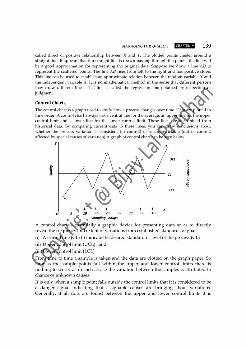
Control Charts

The control chart is a graph used to study how a process changes over time. Data are plotted in

time order. A control chart always has a central line for the average, an upper line for the upper

control limit and a lower line for the lower control limit. These lines are determined from

historical data. By comparing current data to these lines, you can draw conclusions about

whether the process variation is consistent (in control) or is unpredictable (out of control,

affected by special causes of variation).A graph of control chart can be seen below:

A control chart is essentially a graphic device for presenting data so as to directly reveal the frequency and extent of variations from established standards of goals.

(i) A central line (CL) to indicate the desired standard or level of the process (CL)

(ii) Upper control limit (UCL) : and

(iii) Lower control limit (LCL)

From time to time a sample is taken and the data are plotted on the graph paper. So long as the sample points fall within the upper and lower control limits there is nothing to worry as in such a case the variation between the samples is attributed to chance or unknown causes.

It is only when a sample point falls outside the control limits that it is considered to be a danger signal indicating that assignable causes are bringing about variations. Generally, if all dots are found between the upper and lower control limits it is

40 35 30 25 20 15 10 5

A

B

C

D

E

F

G LCL

CL

UCL

H Y

X O

Qu

alit

y

Ch

ara

cter

isti

c

Sampling Groups

Accep

tab

le Ra

ng

e

PRODUCTION AND OPERATIONS MANAGEMENT

assumed that the process is "in control" and only chance causes are present. However, sometimes dots are found arranged in some peculiar way. Although they appear between the control limits, a substantial number of successive dots may be located on the same side of the central line or successive dots may follow a definite path leading towards the upper and lower control limits. Such patterns of dots within control limit should also be considered as danger signals which may indicate a change in the production process.

Flow chart

To find the errors or dissatisfaction of the customer , one must first determine how a process works and what it supposed to do. By clearly defining a process, all involved reach a common understanding and do not waste collecting irrelevant data. Understanding how a process works also enables one to pinpoint obvious problems, error-proof the process and streamline it by eliminating non value added steps. Developing a flow chart of the process usually aid in understanding the error or dissatisfaction. Flow chart are best developed by having the people involved in the process – employees, supervisors, managers and customers-construct a flow chart. A facilitator can guide the discussions through questions such as “What happen next?”, “Who makes decision at that point? And “ What operation performed at that point?”

A flow chart is a graphical or symbolic representation of a process. Each step in the

process is represented by a different symbol and contains a short description of the

process step. The flow chart symbols are linked together with arrows showing the

process flow direction. This diagrammatic representation can give a step-by-step

solution to a given problem. Data is represented in these boxes, and arrows connecting

them represent flow / direction of flow of data. Flowcharts are used in analyzing,

designing, documenting or managing a process or program in various fields. A

specimen of flow chart is given below:

Flow chart help the people who are involved in the process understand it much better and more objectively. Employees realize how they set into the process and who are their suppliers and customers which will lead to improved communications among all concerned. It shows the sequence of events in a process. Flow charts are often used to diagram operational procedures to simplify the system. Once the flow chart is constructed, it can be used to identify quality problems as well as areas of productivity improvement. They can identify bottlenecks, redundant steps and non-value added activities. The flow chart also can be identifies where delays can occur.

MANAGING FOR QUALITY CHAPTER - 9

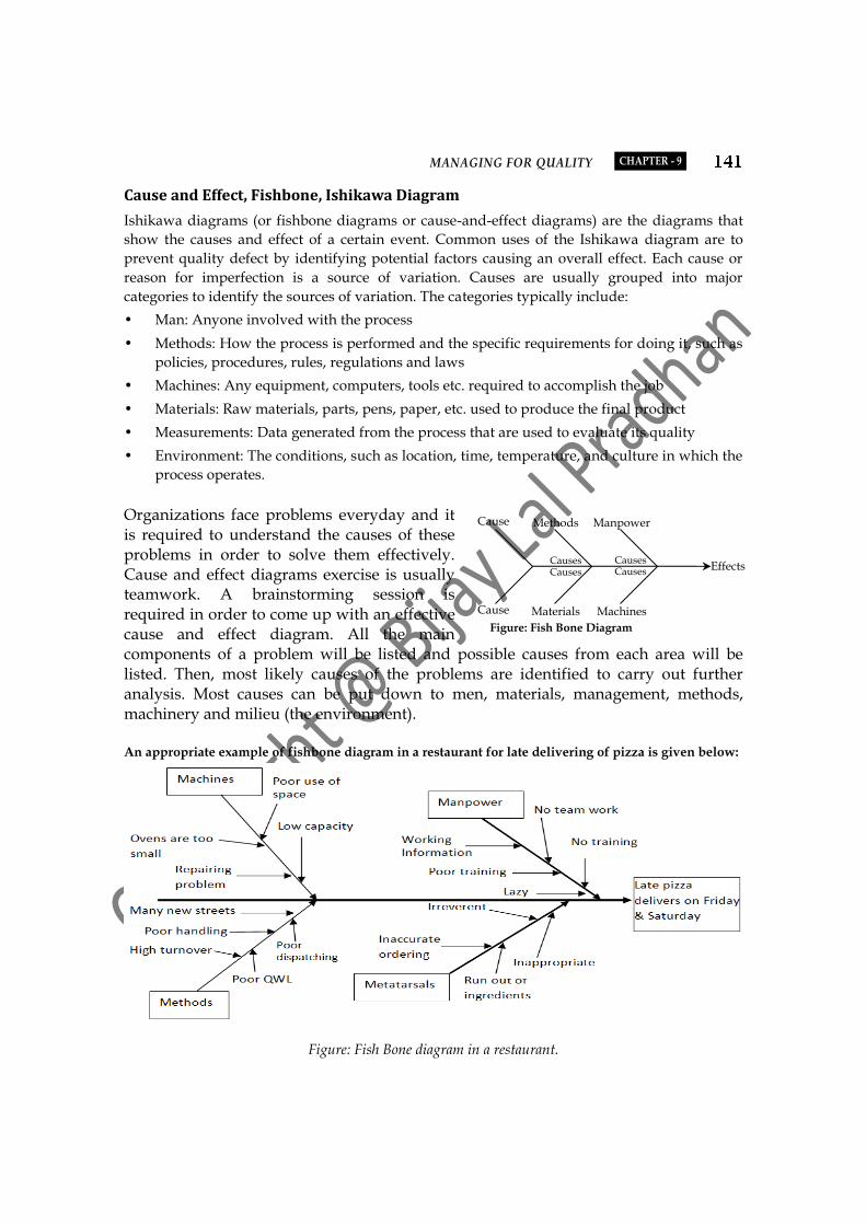
Cause and Effect, Fishbone, Ishikawa Diagram

Ishikawa diagrams (or fishbone diagrams or cause-and-effect diagrams) are the diagrams that

show the causes and effect of a certain event. Common uses of the Ishikawa diagram are to

prevent quality defect by identifying potential factors causing an overall effect. Each cause or

reason for imperfection is a source of variation. Causes are usually grouped into major

categories to identify the sources of variation. The categories typically include:

• Man: Anyone involved with the process

• Methods: How the process is performed and the specific requirements for doing it, such as

policies, procedures, rules, regulations and laws

• Machines: Any equipment, computers, tools etc. required to accomplish the job

• Materials: Raw materials, parts, pens, paper, etc. used to produce the final product

• Measurements: Data generated from the process that are used to evaluate its quality

• Environment: The conditions, such as location, time, temperature, and culture in which the

process operates.

Organizations face problems everyday and it is required to understand the causes of these problems in order to solve them effectively. Cause and effect diagrams exercise is usually teamwork. A brainstorming session is required in order to come up with an effective cause and effect diagram. All the main components of a problem will be listed and possible causes from each area will be listed. Then, most likely causes of the problems are identified to carry out further analysis. Most causes can be put down to men, materials, management, methods, machinery and milieu (the environment).

An appropriate example of fishbone diagram in a restaurant for late delivering of pizza is given below:

Figure: Fish Bone diagram in a restaurant.

Cause Methods Manpower

Cause Materials Machines

Effects Causes Causes

Causes Causes

Figure: Fish Bone Diagram

PRODUCTION AND OPERATIONS MANAGEMENT

Histogram or Bar Graph

A Histogram is a graphic

summary of variation in a set of

data. It enables us to see patterns

that are difficult to see in a simple

table of numbers. It can be

analyzed to draw conclusions

about the set of data.

A histogram is a graph in which

the continuous variable is taken

along with X axis and the

corresponding numbers are

plotted in to the Y axis as given

above. The total area of the histogram is equal to the number of data. Histograms are used to

plot density of data, and often for density estimation of the underlying variable.

Check Sheets

The check sheet is a simple document that is used

for collecting data in real-time and at the location

where the data is generated. The document is

typically a blank form that is designed for the

quick, easy, and efficient recording of the desired

information, which can be either quantitative or

qualitative. When the information is quantitative,

the check sheet is sometimes called a tally sheet.

An example of check sheet is given below:

Check Lists

A checklist is a type of informational job aid used

to reduce failure by compensating for potential

limits of human memory and attention. It helps to

ensure consistency and completeness in carrying

out a task. A basic example is the "to do list." A

more advanced checklist would be a schedule,

which lays out tasks to be done according to time

of day or other factors.

A Checklist contains items that are important or

relevant to a specific issue or situation. Checklists

are used under operational conditions to ensure

that all important steps or actions have been taken.

Their primary purpose is for guiding operations, not for collecting data. It is generally used to

check that all aspects of a situation have been taken into account before action or decision

making.

MANAGING FOR QUALITY CHAPTER - 9

Diagrammatic representation of Seven QC Tools suggested by Isikawa

Inspection is an appraisal activity that compares goods or services to a standard.

Inspection is a vital but often unappreciated aspect of quality control. Although for well-

designed processes little inspection is necessary, inspection cannot be completely

eliminated. And with increased outsourcing of products and services, inspection has taken

on a new level of significance. In lean organizations, inspection is less of an issue than it is

for other organizations because lean organizations place extra emphasis on quality in the

design of both products and processes. Moreover, in lean operations, workers have

responsibility for quality (quality at the source). However, many organizations do not

operate in a lean mode, so inspection is important for them. This is particularly true of

service operations, where quality continues to be a challenge for management.

PRODUCTION AND OPERATIONS MANAGEMENT

Inspection can occur at three points: before production, during production, and after

production. The logic of checking conformance before production is to make sure that

inputs are acceptable. The logic of checking conformance during production is to make

sure that the conversion of inputs into outputs is proceeding in an acceptable manner. The

logic of checking conformance of output is to make a final verification of conformance

before passing goods on to customers.

Inspection before and after production often involves acceptance sampling procedures;

monitoring during the production process is referred to as process control.

To determine whether a process is functioning as intended or to verify that a batch or lot

of raw materials or final products does not contain more than a specified percentage of

defective goods, it is necessary to physically examine at least some of the items in

question. The purpose of inspection is to provide information on the degree to which

items conform to a standard. The basic issues are

1. How much to inspect and how often.

2. At what points in the process inspection should occur.

3. Whether to inspect in a centralized or on-site location.

4. Whether to inspect attributes (i.e., count the number of times something occurs) or

variables (i.e., measure the value of a characteristic).

It is a statistical device principally used for the study and control of According to Dr. Walter A.

Shewhart, control chart may serve, first to defiae me goal or standard for the process that the

management might strive so attain: secondly it may be used as an instrument to attain that goal; and

tturdh, it nay serve as a means of judging whether the goal, is being achieved.

A control chart is essentially a graphic device for presenting data so as to directly reveal the

frequency and extent of variations from established standards of goals.

(i) A central line (CL) to indicate the desired standard or level of the process (CL)

(ii) Upper control limit (UCL) : and

(iii) Lower control limit (LCL)

From time to time a sample is taken and the data are plotted on the graph paper. So long as the

sample points fall within the upper and lower control limits there is nothing to worry as in such a

case the variation between the samples is attributed to chance or unknown causes.

It is only when a sample point falls outside the control limits that it is considered to be a danger

signal indicating that assignable causes are bringing about variations. Generally, if all dots are found

between the upper and lower control limits it is assumed that the process is "in control" and only

chance causes are present. However, sometimes dots are found arranged in some peculiar way.

Although they appear between the control limits, a substantial number of successive dots may be

located on the same side of the central line or successive dots may follow a definite path leading

towards the upper and lower control limits. Such patterns of dots within control limit should also be

considered as danger signals which may indicate a change in the production process.

MANAGING FOR QUALITY CHAPTER - 9

A specimen of the control chart is given below :

The control chart may be likened to a highway whose control limits are the shoulders on the side and

the centre line on the other.

Dr. W.A. Shewhart impressed upon the fact that a manufacturing process should not be deemed to

be in statistical control unless the stable pattern of chance or random variations persist for quite some

time and for a reasonably good amount of production from the process. In his words, "this potential

state of economic control can be approached only as a statistical limit even after the assignable causes

of variability have been detected and removed. Control of this kind cannot be reached in a day. It

cannot be reached in the production of a product in which only a few pieces are manufactured. It

can, however, be approached scientifically in a continuing mass production."

How to Set-up the Control Limits

The control chart is based upon time to time lot to lot or sample to sample the setting up of upper

and lower control limits. These limits are used as a basis of judging the significance of the quality

variations. The moment a point falls outside these limits, it is taken to be a danger signal. The control

limits serve as a guide for action and, therefore, they are also referred to as action limits. Control

limits are established by computation based upon:

(i) Data covering past and current production records.

(ii) Statistical formulate whose reliability has been proved in practice.

Although, the nature of the control problem does not permit standardizing precise and inflexible

rules for computing control limits that will be found suited to the various conditions that may

encounter in actual practice, it has been found possible to develop certain general procedures on the

basis of experience that will cover a wide range of industrial applications.

It has been found satisfactory to place the control limits above and below the grand average of the

statistical measures (–X, , R etc.) that is being plotted at distances of three times a computed value,

commonly designated as the "sigma" of the statistics measure, for sub-groups of the size under

consideration. These are referred to as "3 sigma'' limits. The logic of drawing 3 limits is that in case of

a normal distribution –X + 3 covers 99.73 per sent of the items. In other words, occurrence of events

beyond the limits (–X + 3), provided the events lie on a normal curve, is on the whole nearly 3 out of

L.C.L.

U.C.L.

Average

Quality Scale

Out of control

3 + sigmas

3 – sigmas

Out of control

Sample (sub-group number) 1 2 3 4 5 6 7 8 9 10 11

PRODUCTION AND OPERATIONS MANAGEMENT

1,000 events-an extremely remote chance under normal circumstances. Hence, if points fall outside 3-

sigma limits, they indicate the presence of some assignable cause-all is not due to random causes. It

should be noted that if points fall outside 3-sigma limits, there is good reason for believing that they

point to some factor contributing to quality variation that can be identified.

The selection of standard value (–X, , p etc.,) is probably the most basic problem encountered in

setting up a control procedure. The primary aim is not just to get control, but to get control at a

satisfactory level. A satisfactory selection depends fundamentally upon the needs of the buyer or

user as defined by his specifications. Any questions of cost of production and capability of

manufacturing process must also be taken into accounts in deciding on a level that will be

economical from an average point of view.

Types of Control Charts

The control charts can be divided under two heads :

(i) Control charts of variables, and

(ii) Control charts of attributes

Variables are those quality characteristics of a product which are 'measurable and can be expressed

in specific units of measurement such as diameter of radio knobs which can be measured and

expressed in specific measures per square inch of space, etc. Attributes, on the other hand, are those

product characteristics which are not amendable to measurement. Such characteristics can only be

identified by their presence or absence from the product. Attributes may be judged either by the

proportion of units that are defective or by the number of defects per unit. Thus the data resulting

from inspection of a quality characteristic may take any one of the following forms:

(i) A record of the actual measurements of the quality characteristics for individual articles or

specimens.

(ii) A record of number of articles or specimens inspected and of the number found defective.

(iii) A record of the number of defects that are found in a sample. The number of defects per sample

may be very large compared to the average number of defects per sample.

For purposes of control, data of the first form (i) listed above may be summarised by taking two

statistical measures, the average (–X) and the standard deviation (), or the average (

–X) and the range

(R). Data of the second form (ii) can be summarized in terms of fraction defective (p), and data of

type (iii) can be summarized in terms of number of defects per unit (c).

Setting up a Control Procedure

The manufacturer must take the following preliminary steps in establishing basic procedures for the

operating of quality control programme.

1. Select the quality characteristics that are to be controlled.

2. Analyse the production process to determine the kind and location of probable causes of

irregularities.

3. Determine how the inspection data are to be collected and recorded, and how they are to be

sub-divided.

4. Choose the statistical measures that are to be used in the chart.

The following types of control charts may be used :

MANAGING FOR QUALITY CHAPTER - 9

(a) Control chart for a or R alone. Control chart for R or a is used alone where technical reasons

render control of x unimportant or where control for x 's known to be unjustifiably expensive.

(b) Control chart for p or pn. Chart for p or pn is used when the records of inspection or testing

show merely the number of articles inspected and the number found defective.

(c) Control charts –X and ,

–X and R. Such charts are used when measured values of the quality

characteristics are at hand.

(d) Control chart of –X alone. Control chart for

–X alone is used where experience with control charts

for –X and R, or

–X and has demonstrated that instances of lack of control are almost always

associated with causes that affect –X rather than or R.

Control charts of the first three types are known as the control charts for variables and last two types

as control charts for attributes.

–X Chart

The –X chart is used to show the quality averages of the samples drawn from a given process.

Compute the following values before constructed the –X chart :

(1) Calculate the mean of each sample, i.e., –X1,

–X2,

–X3 etc. This is done by dividing the sum of the

values included in a sample (X) by the number of items in the sample (n or sample size)

=X =

–X

n

(2) Obtain the mean of the sample means, i.e., =X. This 's done by the sum of the sample means (

–X)

by the number of samples to be included in the chart.

=X =

–X

Number of samples

(3) The control limits are set at

U.C.L. = =X + 3

–X

L.C.L. = –X – 3

–X

Where x =

n

and = d' –R

–R is a biased estimator of and d' is the correction factor. The values of d' are tabulated and are

given in the appendix at the end of the book.

Therefore, the control limits are

U.C.L. = =X + A2

–R

L.C.L. = –X – A2

–R

PRODUCTION AND OPERATIONS MANAGEMENT

R Chart

It is used to show the variability or dispersion of the quality produced by a given process. R chart (or

a chart) is the companion chart to –X chart and both are usually required for adequate analysis of the

production process under study. The R chart is generally presented along with the –X chart. The

general procedure for constructing the R chart is similar to that for the –X chart. The required 'values

for constructing the R chart are:

(1) The range of each sample, R

(2) The mean of the sample ranges, –R

(3) U.C.L. and L.C.L.

U.C.L.R = –R + 3R; and

L.C.L.R = –R – 3R Where, R= the standard error of the range.

The value of sR may be estimated by finding the standard deviation of the ranges of the samples

included in a chart, in practice, however, it is rather convenient to compute the upper and lower

control limits by using the. values D4 and D3 as provided in Appendix given towards the end of the

book-statistical tables according to various sample sizes (n = 2 to 20). When the tabulated vales are

used, the two limits may be written as follows:

U.C.L.R = D4 –R

L.C.R.R = D3

–R

It should be noted that the use of R chart is recommended only for relatively small samples sizes

(rarely more than 12 to 15 units). For the large samples sizes (n > 12) the a chart is to be processed.

Control Chart for the Standard Deviation or -Chart

We also use control chart for –X and for controlling process average and variability. In fact, since

standard deviation is considered to be an ideal measure of dispersion, control chart for –X and is

theoretically more appropriate than control chart for –X and R. The 3 control limits for control chart

for standard deviation are given by:

U.C.L. = B2

L.C.L. = B1

where is process standard deviation. If a is not known then its estimate based on the average of

sample standard deviations is used. In that case:

U.C.L. = B4 –S

L.C.L. = B3 –S

Where

–S =

Sum of the sample standard deviationNumber of samples

The steps in the construction of chart and its interpretation is on the same lines as R-chart.

MANAGING FOR QUALITY CHAPTER - 9

Example 1 The table below gives the (coded) measurements obtained in 20 samples (sub-groups). Construct control charts based on the mean and the range. The values of these statistics are given below for the respective samples.

Sub groups

1 2 3 4 5 6 7 8 9 10 11 12 13 14 15 16 17 18 19 20

–1

2

1

0

1

2

0

1

0

1

1

1

0

0

1

2

1

0

1

0

1

–1

0

0

–1

1

–1

2

0

–2

–1

1

0

–2

1

1

1

2

–1

0

2

1

–1

0

0

–2

1

–2

2

1

0

1

–3

2

1

2

1

–1

0

0

0

1

–3

2

1

0

0

–1

0

1

–1

2

1

1

2

1

–1

2

0

–2

2

1

–1

0

0

2

0

1

0

1

0

2

1

–1

1

3

–3

–1

1

2

–X 6 8 6 4 -2 0 -6 6 4 0 2 4 2 0 1 9 9 4 6 4

R 3 1 1 3 2 4 3 3 3 4 5 3 5 2 3 4 3 2 3 6

Solution

–X =

X1 + X2 + . . . + –Xn

n1 + n2 + n3 + nn

= .6 + .8 + .6 + .4 - .2 + 0 - .6 + .6 + .4 + 0 + .2 + .4 + .2 + 0 + 1.0 + 0 + .4 + .8 + .6 + .4

20 = 6.620 = 0.33

–R =

3 + 1 + 1 + 3 + 2 + 4 + 3 + 3 + 3 + 4 + 5 + 3 + 5 + 3 + 2 + 3 + 4 + 3 + 2 + 3 + 620 =

6320 = 3.15

From the table for the sample of size 5, we find that

A = 0.577, D3 = 0 and D4 = 2.115

Upper and lower control limits for –X chart =

–X + A2

–X

= 0.33 + 0.577 (3.15) = 0.33 + 1.818

Lower control limit = 0.33 – 1.818 = - 1.488

Upper control limit = 0.33 + 1.818 = - 2.148

Upper and lower control limits for R chart

U.C.L. = D4

–R = 2.115 (3.15) = 6.662

L.C.L. = D3 –X = 0(3.15) = 0

The following two control charts are prepared with the help of the above control limits.

Mea

sure

men

ts

Control chart for –X

Sub-group 2 4 6 8 10 12 14 16 18 20

–3

–2

–1

0

1

2

3 UCL = 2.148

CL = 0.33

LCL = 1.488

PRODUCTION AND OPERATIONS MANAGEMENT

The fact that in both graphs all sample points are falling within the 3-sigma control limits can be interpreted as implying that the process is in a state of statistical control or, in other words, that the only kind of variation present in chance variations.

Example 2 A drilling machine bores holes with a mean diameter of 0.5230 cm and a standard deviation of 0.0032 cm. Calculate the 2-sigma and 3-sigma upper and lower control limits for means of samples 4, and prepare a control chart.

Solution

We have, =X = 0.5230 cm, = 0.0032 cm, n = 4

n =

0.00322 = 0.0016

2-sigma limits for means of samples of 4:

UCL = –X = 2(/ n) UCL = 0.5230 + 2(0.0016) = 0.5262 cm

Central line = 0.5230 cm

LCL = =X – 2(/ n)

= 0.5230 – 2(0.0016) = 0.5198 cm

3-sigma limits for means of sample of 4

UCL = =X + 3(/ n)

= 0.5230 + 3(0.0016) = 0.5278 cm

Central line = 0.5230

LCL = –X + 3(/ n)

= 0.5230 – 3(0.0016) = 0.5182 cm

Example 3 A food company puts mango juice into cans advertised as containing 10 ounces, of the juice. The weights of the juice drained from cans immediately after filling for 20 samples are taken by a random method (at an interval of every 30 minutes). Each of the samples includes 4 cans. The samples are tabulated in the following table. The weights in the table are given in units of 0.01 ounces in excess of 10 ounces. For example, the weight of juice drained from the first can of the sample is 10.15 ounces which is in excess of 10 ounces excess being 0.15 ounces (10.15 - 10 = 0.15).

Mea

sure

men

ts

Control chart for R

Sub-group 2 4 6 8 10 12 14 16 18 20

–4

–2

0

2

4

6

8 UCL =6.662

CL = 3.15

LCL = 0

LCL (3)

LCL (2)

Central line

LCL (2)

LCL (3) (0.5278) B

(0.5262) A

(0.5230) 0

(0.5198) A'

(0.5182) B'

MANAGING FOR QUALITY CHAPTER - 9

Since the unit in the table is 0.01 once, the excess is recorded as 15 units in the table. Construct a –X

chart to control the weights of mango juice for the filling.

Sample Number Weight of each can (4 cans in each sample, n = 4–X)

1 2 3 4 5 6 7 8 9 10 11 12 13 14 15 16 17 18 19 20

15 10 8 12 18 20 15 13 9 6 5 3 6 12 15 18 13 10 5 6

12 8 15 17 13 16 19 23 8 10 12 15 18 9 15 17 16 20 15 14

13 8 17 11 15 14 23 14 18 24 20 18 12 15 6 8 5 8 10 33

20 14 10 12 4 20 17 16 5 20 15 18 10 18 16 15 4 10 12 14

Solution

Calculation for –X chart

Sample number

Weight of each can (4 cans in each

sample, n = 4–X)

Total weight of 4

cans X

Sample mean

(–X = X/4)

Sample range (L-S)

1 2 3 4 5 6 7 8 9 10 11 12 13 14 15 16 17 18 19 20

15 10 8

12 18 20 15 13 9 6 5 3 6

12 15 18 13 10 5 6

12 8

15 17 13 16 19 23 8

10 12 15 18 9

15 17 16 20 15 14

13 8

17 11 15 14 23 14 18 24 20 18 12 15 6 8 5 8

10 33

20 14 10 12 4 20 17 16 5 20 15 18 10 18 16 15 4 10 12 14

60 40 50 52 50 70 74 66 40 60 52 54 46 54 52 58 38 48 42 46

15.0 10.0 12.5 13.0 12.5 17.5 18.5 16.5 10.0 15.0 13.0 13.5 11.5 13.5 13.0 14.5 9.5

12.0 10.5 11.5

8 6 9 6 14 6 8 10 13 18 15 15 12 9 10 10 12 12 10 8

Total 263.0 211

PRODUCTION AND OPERATIONS MANAGEMENT

Calculations:

1. The mean of the sample means (=X) = 263/20 = 13.15

2. The mean of the range value (–R) = 211/20 = 10.55

3. Control limits:

CL = =X= 13.15

UCL = =X + A2

–R = 13.15 + 0.729 × 10.55 = 13.15 + 7.69 20.84

LCL = =X – A2

–R = 13.15 – 0.729 × 10.55 = 5.46

Since all the points are falling within control limits the process is in a state of control and hence there

is nothing to worry.

Control Chart for P (fraction defective)

The p-chart is deigned to control the percentage or proportion of defectives per sample. Since the

number of defectives (c) can be converted into a percentage expressed as a decimal fraction merely

by dividing c by the sample size, the p-chart may be used in place of the c-chart. The p-chart has at

least two advantage over the c-chart.

(1) Expressing the defectives as a percentage or fraction of production is more meaningful and

more generally understood than would be the statement of. the number of defectives. The latter

concept must be related in some way to the total number produced.

(2) Where the size of the sample varies from sample to sample, the p-chart permits a more

straightforward and less cluttered presentation. The p-chart requires, however, that the division

c/n be made. This additional computation may be regarded as a slight disadvantage.

The same basic data is used for body c as well as p chart. When the sample size remains constant

from sample to sample, the primary difference lies in the computation of the control limits. The c-

chart control limits are set at c plus or minus three standard deviations. The p-chart control limits are

set at p plus or minus three standard errors of the proportion.

This chart has its theoretical basis in the binomial distribution, and generally gives best results when

the sample size is large, say, at least 50. The steps in constructing the chart are :

(i) Compute the average fraction defective (–p) by dividing the number of defectives by the total

number of units inspected.

Mea

sure

men

ts

Control chart for –X

Sample no. 2 4 6 8 10 12 14 16 18 20

5

UCL = 20.8

CL = 13.15

LCL = 5.46

10

15

20

MANAGING FOR QUALITY CHAPTER - 9

(ii) On the chart draw a solid horizontal line to represent p.

(iii) Determine the upper and lower control limits. The upper and lower control limits are obtained

by the average fraction defective plus and minus three times and standard error as follows :

U.C.L. = –p + 3

–p (1 -

–p)

n L.C.L. = –p – 3

–p (1 -

–p)

n

While constructing the chart, it is generally preferred to express results in terms of 'per cent

defective' rather than 'fraction defective'. The per cent defective is 100 p. Any sample point falling

outside the control limits is evidence of a possible lack of control inasmuch as the probability of

getting such value by chance is less than 0.003.

Example 4 Construct a control chart for the proportion of defectives obtained in repeated random samples of size 100 from a process which is considered to be under control when the proportion of defective p is equal to 0.20. Draw the control line and the upper and the lower control limits on graph paper.

We are given,

–p = average fraction defective = 0.2, n = 100

–p (1 -

–p)

n = 0.20 × 0.80

100 = 0.0016 = 0.40

U.C.L. = –p + 3

–p (1 -

–p)

n = 0.20 + 3(0.04) = 0.32

Central line = –p = 0.20

L.C.L. = –p - 3

–p (1 -

–p)

n = 0.20 – 3(0.04) = 0.08

Since the number of defectives can not be negative, L.C.L. is taken as zero.

Example 5 The following table gives the inspection data on completed spark plugs:

Lot No. Number defectives

Fraction defectives

Lot. No. Number defectives

Fraction defectives

1

2

3

4

5

6

7

8

9

10

5

10

12

8

6

5

6

3

3

5

0.050

0.100

0.120

0.080

0.060

0.050

0.060

0.030

0.030

0.050

11

12

13

14

15

16

17

18

19

20

4

7

8

2

3

4

5

8

6

10

0.040

0.070

0.080

0.020

0.030

0.040

0.050

0.080

0.060

0.100

Construct an appropriate control chart.

Solution

Since we are given fraction defectives, the suitable chart will be p-chart. Calculation for p-chart are

1. Average fraction defective, i.e.

LCL = 0.08

CL = 0.20

UCL = 0.32 (0.32)

(0.20)

(0.08)

Control chart for proportion defects

PRODUCTION AND OPERATIONS MANAGEMENT

–p =

dm×n =

12020 × 100 =

1202000 = 0.06

2. UCL = –p + 3

–p(1 -

–p)

n = 0.06 + 30.06(1 - 0.06)

100 = 0.1311

3. LCL = –p – 3

–p(1 -

–p)

n = 0.06 – 30.06(1 - 0.06)

100 = – 0.111

Since the fraction defective cannot be negative, the LCL is take zero.

The control chart shows that all the points are falling within control limits. Hence the process is in a state of control.

In order to simplify the work of the person who plots the necessary points on the control charts, the above chart can be modified so that he can directly plot the number rather than' the fraction or percentage of defectives. Such a chart is called the Control Chart for number of defectives. To obtain such a chart the central line as well as the control limits are multiplied by n. The central line thus becomes np and the control limits are :

n–p + 3 n

–p (1 -

–p)

Example 6 The following data refer to visual defects found in the inspection of the first 10 samples of size 100. Use the data to obtain upper and lower control limits for percentage defective in samples of 100. Represent the first ten sample results in the chart you prepare to show the central line and control limits:

Sample No. 1 2 3 4 5 6 7 8 9 10 Total

No. of defectives 2 1 1 3 2 3 4 2 2 0 20

Solution

Since there are 20 defective items in 10 samples each of size 100, therefore –p = average fraction

defective = 20

10 × 100 = 0.02

Also, n = 100

n –p = 100 × 0.02 = 2

and n–p (1 –

–p) = 100 × 0.02 × 0.98 = 1.96 = 1.4

UCL = n–p + 3 n

–p (1 –

–p) = 2 + (3 × 1.4) = 6.2

Central line = up = 2

P = 0.06

UCL = 0.131

2 4 6 8 10 12 14 16 18 20 O

.02

.04

.06

.08

.10

.12

Fra

ctio

n d

efec

tiv

e

.14

Lot number

MANAGING FOR QUALITY CHAPTER - 9

UCL = n–p – 3 n

–p (1 –

–p) = 2 – 3(1.4) = 2.2

LCL is taken zero as number of defectives cannot be negative.

A critical aspect of statistical quality control is evaluating the ability of a production

process to meet or exceed preset specifications. This is called process capability. To

understand exactly what this means, let’s look more closely at the term specification.

Product specifications, often called tolerances, are preset ranges of acceptable quality

characteristics, such as product dimensions. For a product to be considered acceptable, its

characteristics must fall within this preset range. Otherwise, the product is not acceptable.

Product specifications, or tolerance limits, are usually established by design engineers or

product design specialists.

Specifications for a product are preset on the basis of how the product is going to be used

or what customer expectations are. Any production process has a certain amount of

natural variation associated with it. To be capable of producing an acceptable product, the

process variation cannot exceed the preset specifications. Process capability thus involves

evaluating process variability relative to preset product specifications in order to

determine whether the process is capable of producing an acceptable product.

Commonly used terms refer to the variability of process output are as follows:

Specifications or tolerances are established by engineering design or customer

requirements. They indicate a range of values in which individual units of output must fall

in order to be acceptable.

2

4

6

UCL = 6.2

CL = 2

Sample no. 1 2 3 4 5 6 7 8 9 10

No

. o

f d

efec

ti\

s Control chart for number of defectives

0

LCL = 0

PRODUCTION AND OPERATIONS MANAGEMENT

Control limits are statistical limits that reflect the extent to which sample statistics such as

means and ranges can vary due to randomness alone.

Process variability reflects the natural or inherent (i.e. random) variability in a process. It

is measured in terms of the process standard deviation.

Process Capability refers to the inherent variability of process output relative to the

variation allowed by the design specifications.

Measuring process Capability

Simply setting up control charts to monitor whether a process is in control does not

guarantee process capability. To produce an acceptable product, the process must be

capable and in control before production begins.

Process potential, Cp

Process capability is measured by the process capability index, Cp, which is computed as

the ratio of the specification width to the width of the process variability: where the

specification width is the difference between the upper specification limit (USL) and the

lower specification limit (LSL) of the process. The process width is computed as 6

standard deviations (6σ) of the process being monitored. The reason we use 6σ is that

most of the process measurement (99.74 percent) falls within 3 standard deviations,

which is a total of 6 standard deviations.

There are three possible ranges of values for Cp that also helps us interpret its value:

Cp=1: A value of Cp equal to 1 means that the process variability just meets specifications.

We would then say that the process is minimally capable.

Cp<1: A value of Cp below 1 means that the process variability is outside the range of

specification. This means that the process is not capable of producing within specification

and must be improved.

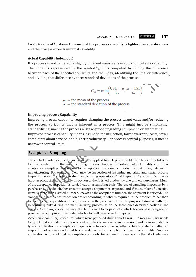
MANAGING FOR QUALITY CHAPTER - 9

Cp>1: A value of Cp above 1 means that the process variability is tighter than specifications

and the process exceeds minimal capability

Actual Capability Index, CpK

If a process is not centered, a slightly different measure is used to compute its capability.

This index is represented by the symbol Cpk. It is computed by finding the difference

between each of the specification limits and the mean, identifying the smaller difference,

and dividing that difference by three standard deviations of the process.

Improving process Capability

Improving process capability requires changing the process target value and/or reducing

the process variability that is inherent in a process. This might involve simplifying,

standardizing, making the process mistake-proof, upgrading equipment, or automating.

Improved process capability means less need for inspection, lower warranty costs, fewer

complaints about service, and higher productivity. For process control purposes, it means

narrower control limits.

The control charts described above cannot be applied to all types of problems. They are useful only

for the regulation of the manufacturing process. Another important field of quality control is

acceptance sampling. Inspection for acceptance purposes is carried out at many stages in

manufacturing. For example, there may be inspection of incoming materials and parts, process

inspection at various points in the manufacturing operations, final inspection by a manufacturer of

his own product, and ultimately inspection of the finished product by one or more purchasers. Much

of the acceptance inspection is carried out on a sampling basis. The use of sampling inspection by a

purchaser to decide whether or not to accept a shipment is inspected and if the number of defective

items is more than a stated number, known as the acceptance number, the shipment is rejected. The

standards in acceptance inspection are set according to what is required to the product, rather than

by the inherent capabilities of the process, as in the process control. The purpose it dons not attempt

to control quality during the manufacturing process, as do the techniques described earlier in the

chapter. Sampling inspection may also be referred to as product control, because it is designed to

provide decision procedures under which a lot will be accepted or rejected.

Acceptance sampling procedures which were perfected during world war II to meet military needs

for quick and accurate inspection of vast supplies or materials, are now used widely in industry. A

typical application of acceptance inspection is to determine whether a batch of items, called an

inspection lot or simply a lot, tat has been delivered by a supplier, is of acceptable quality. Another

application is to a lot that is complete and ready for shipment to make sure that it of adequate

PRODUCTION AND OPERATIONS MANAGEMENT

quality. Still another application is in the case of partly completed material, to determine whether the

lot is of sufficiently high quality of justify further processing.

Role of Acceptance Sampling

Acceptance sampling is very widely used in practice because of the following reasons:

Acceptance sampling is much less expensive than 100 per cent inspection.

In many cases it provides better outgoing quality. It is generally agreed that good 100 per cent

inspection will remove only about 85 to 95 per cent of the defective items but still not reach 100

per cent. Because of the effect of inspection fatigue involved in 100 per cent inspection, a good

sampling plan may actually give better quality assurance than 100 per cent inspection. The word

‘good’ is italicized since many informal sampling plans devised without knowledge of the laws of

chance are practically worthless. Hence, there is a need for devising an appropriate acceptance

sampling plan.

In modern manufacturing plants, acceptance sampling is used for evaluating the acceptability of

incoming lots of raw materials and parts at various stages of manufacture, and final inspection of

finished product.

Where quality can be tested only by destroying items, as in determining the strength of glass

containers, 100 per cent inspection is out of the question and sampling must be used. Of course,

there are situations where 100 per cent inspection is not to be put aside; for example, in testing

rifles to be used by soldiers, we cannot risk imperfection in any item and therefore must test each

and every rifle.

Producers Risk and Consumers Risk

Since under a sampling inspection plan a decision is made as to whether to accept a lot or reject a

lot on the basis of a sample, there is a possibility of (1) rejecting a lost as satisfactory when it is a

fact it is a fact it is below the quality level. Hence in any acceptance sampling plan the producers

and the consumers, te seller and te buyers, are exposed to some risks which are called producer’s

and consumer’s risks. The producer’s risk is the risk a producer takes that a lot will be rejected a

sampling plan even though it confirms to requirements. This is equivalent to the concept of type I

error, or the probability of rejecting hypothesis when it is in fact true. The consumer’s risk is the

risk that a lot of certain bad quality will be accepted by a sampling plan. It is equivalent to type II

error which is the probability of accepting a hypothesis when an alternative is true. Before

agreeing to an acceptance criterion the consumers and producers will like to know the risks to

which they are exposed, i.e., the probability of rejecting a good lot and the probability of

accepting a bad one.

An inspection plan can easily be constructed if the consumers and producers specify these

probabilities and also the proportion of defectives above which a log is considered to be bad and

the proportion of defectives below which a lot is considered to be good.

Types of Acceptance Sampling Plans

The three types of acceptance sampling plans are commonly used:

Single sampling plan: When the decision whether to accept a lot or reject a lot is made on the basis

of only one sample, the acceptance plan is described as a single sampling plan. This is the simplest

type of sampling plan. In any systematic plan for single sampling three things are specified, namely,

(a) Number of items N in the lot from which the sample is to be drawn. (b) Number of articles n in

the random sample drawn from the lot. (c) The acceptance number c. This acceptance number is the

MANAGING FOR QUALITY CHAPTER - 9

maximum allowable number of defective articles in the sample. More than this number will cause

the rejection of the lot. Thus a sampling plan may be specified in this way.

N = 200 C = 1

These three numbers may be interpreted as saying “Take a random sample of 20 from a lot of 200. If

the sample contains more than 1 defective, reject the lot; otherwise accept the lot”

Double Sampling Plan: In the single sampling plan discussed above, decision with regard to

acceptance or rejection of a lot is based on te evidence of only one sample from the lot. However,

double sampling involves the possibility of putting of the decision on the lot until a second sample

has been taken. A lot may be accepted at once if the first sample is good enough or rejected at once if

the first sample is bad enough. If the first sample is neither good enough nor bad enough, the

decision is based on the evidence of the first and second samples combined. In a double sampling

plan 5 things are specified:

n1, c1, n2, (n1+n2) and c2

n1 = number of pieces in the first sample.

c1 = acceptance number of the first sample (the maximum number of defectives that will permit the

acceptance of the lot on the basis of the first sample).

n2 = number of pieces in the second sample.

n1+n2= Number of pieces in the two samples combined.

C2 = Acceptance number for the two sample combined (the maximum number of defectives that will

permit the acceptance of the lot on the basis of the two samples).

Thus a double sampling plan may be:

N=500 N1=20 C1=1 N2=60 C2=4

This will be interpreted as follows:

Inspect a first sample of 20 from a lot of 500

Accept the lot on the basis of the first sample if it contains 1 defective.

Reject the lot on the basis of the first sample if the sample contains more than 1 defective.

Inspect a second sample of 60 if the first sample contains 2, 3, 4 defectives.

Accept the lot on the basis of combined sample of 80 in the combined sample contains 4 or less

defectives.

Reject the lot on the basis of combined sample if the combined sample contains more than 4

defectives.

Advantages of Double Sampling Plan

A double sampling plan has two possible advantages over a single sampling plan:

It may reduce that the total amount of inspection. The first sample taken is less tan that called for

under a comparable single sampling plan and consequently, in all cases in which a lot is accepted

or rejected on the basis of first sample, there may be considerable saving in total inspection. It is

also possible to reject a lot without completely inspecting the entire second sample.

A double sampling plan has the psychological advantage of giving a lot a second chance. To

some people, especially the producer, it may seem unfair to reject a lot on the basis of a single

sample. Double sampling permits the taking of two samples on which to make a decision.

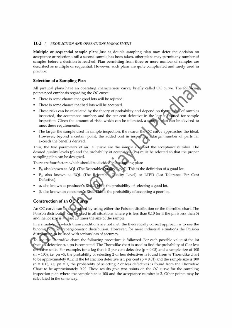
PRODUCTION AND OPERATIONS MANAGEMENT

Multiple or sequential sample plan: Just as double sampling plan may defer the decision on

acceptance or rejection until a second sample has been taken, other plans may permit any number of

samples before a decision is reached. Plan permitting from three or more number of samples are

described as multiple or sequential. However, such plans are quite complicated and rarely used in

practice.

Selection of a Sampling Plan

All piratical plans have an operating characteristic curve, briefly called OC curve. The following

points need emphasis regarding the OC curve:

There is some chance that good lots will be rejected.

There is some chance that bad lots will be accepted.

These risks can be calculated by the theory of probability and depend on the number of samples

inspected, the acceptance number, and the per cent defective in the lots submitted for sample

inspection. Given the amount of risks which can be tolerated, a sample plan can be devised to

meet these requirements.

The larger the sample used in sample inspection, the nearer the OC curve approaches the ideal.

However, beyond a certain point, the added cost in inspecting a larger number of parts far

exceeds the benefits derived.

Thus, the two parameters of an OC curve are the sample size and the acceptance number. The

desired quality levels (p) and the probability of acceptance (Pa) must be selected so that the proper

sampling plan can be designed.

There are four factors which should be decided in a sampling plan:

P1, also known as AQL (The Rejectable Quality Level). This is the definition of a good lot.

P2, also known as RQL (The Rejectable Quality Level) or LTPD (Lot Tolerance Per Cent

Defective).

α, also known as producer’s Risk. This is the probability of selecting a good lot.

β, also known as consumer’s Risk. This is the probability of accepting a poor lot.

Construction of an OC Curve

An OC curve can be determined by using either the Poisson distribution or the thornlike chart. The

Poisson distribution can be used in all situations where p is less than 0.10 (or if the pn is less than 5)

and the lot size is at least 10 times the size of the sample.

In a situation in which these conditions are not met, the theoretically correct approach is to use the

binomial or the hypergeometric distribution. However, for most industrial situations the Poisson

distribution ca be used with serious loss of accuracy.

To use the Thorndike chart, the following procedure is followed. For each possible value of the lot

fraction defective p, a pn is competed. The Thorndike chart is used to find the probability of C or less

defective units. For example, for a log that is 5 per cent defective (p = 0.05) and a sample size of 100

(n = 100), i.e, pn =5, the probability of selecting 2 or less defectives is found from te Thorndike chart

to be approximately 0.12. If the lot fraction defective is 1 per cent (p = 0.01) and the sample size is 100

(n = 100), i.e, pn = 1, the probability of selecting 2 or less defectives is found from the Thorndike

Chart to be approximately 0.92. These results give two points on the OC curve for the sampling

inspection plan where the sample size is 100 and the acceptance number is 2. Other points may be

calculated in the same way.

MANAGING FOR QUALITY CHAPTER - 9

Quality circle means a team established to improve the quality of manufactured products. The

concept is based on the premise that those working closet to the process are likely to have greatest

insight into the improvement of way it is produced. This will be further enhanced if people work

together as a team rather than as individuals. This nature and composition of the team depends on

the particular circumstances.

Conditions necessary for the success of quality circles

The success of quality circles depend the following conditions:

Active support and commitment on the part of top level management.

Proper coordination in the team.

Commitment and ability of facilitators and leaders, and

Proper education about the quality circle philosophy and sufficient for facilitators, leaders and members.

The techniques of quality circles involve individual workers to work together in problem-solving

process. The aim is to involve employees to actively participate in improvement process. As no work

environment can expected to be perfect, the people who face the problems are expected to identify,

investigate and find solutions to the problems. As such this concept envisages the involvement of

rank and files employees no employee should feel unwelcome to get involved in a circle. Employee

participation may however depend upon the attitude of the employees and the time at his disposal.

Employees from the same work area are grounded in a circle. Although no limit is laid down to the

number, an effective working of the circle requires around 10 members. The members meet regularly

for about one hour every week, a superior who initially volunteers to start the circles may lead the

same. A circle starts functioning after developing a program, which is a detailed procedure, also

called as quality circle cycle. The program lists the different topics of discussion and the action taken.

The activities and the results of the circle then are put forth for a management review.

Quality circle increase the involvement of employees by means of participation. It provides an

environment of creativity and achievement. To employees, it provides an opportunity to train and

develop. By mutual exchange of ideas, they reach full potential, work becomes more enjoyable and

purposeful. When workers and different levels of management are brought together, communication

is improved.

From the organizational point of view the advantage are mainly two folds: firstly, quality circles

mark a commitment of companies to change the organizational culture. Secondly, it enhances of

effectiveness business. It provides an answer to the question, how to manage human resources for

business improvement.

Process involved in Quality Circles

The process of quality circles involve the following steps:

Identification of problem: The members may able to identify several problems in their area. Quality,

productivity, cost reduction, housekeeping and safety are some of the general categories of problems

which may be identified by quality circle. Techniques, such as brainstorming, may be used to help

problem identification.

Problem selection: Problem selection is a prerogative of the circle. When several problems are

identified, a selection of the problem for further process of the quality circle may become necessary.

PRODUCTION AND OPERATIONS MANAGEMENT

Problem analysis: The circle members analyses the selected problems. If needed, the circle may take

the assistance of experts and consultants.

Recommendation to the top-management: Finally, the circle makes its recommendations to its

departmental heads in the first instance, normally once in 7-8 weeks selected cases of all circles are

presented to the top management, normally once in 2-3 months, known as management

presentation. In a management presentation, the leader and member describe to their manager what

project they have been working on and what recommendations they wish to make regarding this.

It is the top management which decides whether the recommendations should be accepted and

implemented.

Constituents of Quality Circles

The various constituents of quality circles are as follows:

Top management: Top management consists of the executive at the higher level. Without an

enthusiastic support from the management, a quality circle cannot be expected to succeed for

continuous growth of programmes, management must support circles by

Providing assistance in training,

Providing accommodation for circle meeting,

Publishing circle activities,

Giving assistance in implementation of approved solutions, and

Giving explanation where circle solution is rejected.

Steering committee: A steering committee is at the highest level of the division or unit. This

committee is headed by a top executive of that division or unit. He is designed as the chairman of the

committee. Some of the functions of this committee include

The promotion of quality circle movement,

The formulation of rules and regulations governing quality circles. The same must be reviewed

periodically.

To look after the progress and activities of quality circles. In case of expansion of quality circles

they must be controlled by splitting into circles. The committee must lay down the rules for these.

Expenses for the functioning of the quality circles like training, expenses towards provisions of

meeting facilities, pointing of documents, etc., have to be sanctioned by the committee.

An annual quality circle convention must be organized. All circle presentation must be

assembled. Selection of the best presentation is done by the committee, and

Evaluation of the progress of the quality circle must be periodically undertaken on the basis of

quality improvement, cost reduction, product innovation, work satisfaction, communication,

team spirit, attitude.

The facilitator: the facilitator plays an important role in the structure of quality circle. He is

responsible for conducting all circle activities. His functions include.

Liaisoning with the coordinator in all quality circle activities,

Execution of all quality circle policies, procedures and code of conduct,

Forwarding of monthly reports of quality circles assigned to him and to the coordinator, and

Arranging for assistants from other departments for quality circles assigned to him.

MANAGING FOR QUALITY CHAPTER - 9

Circle leader: The circle leader is to be chosen by the members of the quality circle. Due to lack of

training on the part of workers, a foreman or supervisor may be initially chosen as a circle leader.

Subsequently, members may decide to have leaders by rotation. His functions include:

To lead the circle

To encourage member to participate,

To provide agenda of the meeting,

To make regular progress report,

To present work solutions made by the circle to the steering committee though the facilitator, and

To ensure that the code of conduct is followed.

Non-members: workers, who are reluctant or unwilling to join a circle, are non-members,

nevertheless, they must be encouraged to give suggestions to circle members.

Coordinator: The coordinator regulates the circle activities throught the organization. An executive

from the quality assurance department is usually given this task. His duties include

Implementation of all policies, rules and regulations laid down by the steering committee,

Coordination of quality circle activities of all the facilitators,

Making arrangements for training of members, leaders and facilitators,

Maintaining all records of activities and monthly reports of quality circles, and

Communication with all the employees on matters relating to the programme.

Example 7 If the average fraction defective of large sample or products is 0.1537. Calculate the control limits. (Given that sub-group size is 2,000)

What modification do you need if the sub-group size is not constant?

Solution:

Since we are given average fraction defective, we will draw p-chart and control limits of p-chart.

Lower Control Limits

LCL = –p – 3

–p(1 -

–p)

n = 0.1537 = 0.1537 - 30.1537(1 - 1537)

2000 = 0.12952 or 0

Upper control limit

UCL = –p +

–p(1 -

–p)

n = 0.1537 + 0.2418 = 0.17788

Central line = 5810 = 5.8

UCL = 2.115 × 5.8 = 5.8

LCL = 0 × 5.8 = 0

Since none of the points lies outside the control limits, the range is in a state of control.

Example 8 A machine is set to deliver packets of a given weight. 10 sample of size 5 each were recorded. Below are given relevant data:

Sample no. 1 2 3 4 5 6 7 8 9 10

PRODUCTION AND OPERATIONS MANAGEMENT

Mean (–X)

15 17 15 18 17 14 18 15 17 16

Range (R) 7 7 4 9 8 7 12 4 11 5

Calculate the values for the central line and the control limits for mean chart and then comment on the state of control.

(Conversion factors for n = 5 are A2 = 0.577, D3 = 0, D4 = 2.115)

Solution

Determining control limits for –X chart.

Sample no. 1 2 3 4 5 6 7 8 9 10 N = 10

Mean (–X)

15 17 15 18 17 14 18 15 17 16

–X = 162

Range (R) 7 7 4 9 8 7 12 4 11 5 R = 74

Central line (=X) =

16210 = 16.2

UCL = –X + A2

–R = 16.2 + 0.577 × 7.4 = 16.2 + 4.27 = 20.47 [

... –R = 74/10 = 7.4]

UCL = –X – A2

–R = 16.2 – 0.577 × 7.4 = 16.2 – 4.27 = 11.93

Since all the points are lying between upper and lower control limits the process is in a state of control.

Example 9 Each of 20 lots of rubber belts contains 200 rubber belts. Numbers of defective rubber belts in those lots are 410, 420, 324, 332, 292, 310, 282, 300, 320, 296, 292, 392, 432, 294, 324, 220, 400, 258, 460, 280.

Calculate control limits for fraction defective chart and give your conclusions.

Solution

Total number of defectives out of 40,000 items in 200 sample is

292 + 310 + 282 + …… + 280 = 6572

–p =

dm×n =

657220 × 200 = 0.1643

Central line = –p = 0.1643

UCL = –p + 3

–p(1 -

–p)

n = 0.1643 + 30.1643 × 0.8357

2000 = 0.1643 + 0.0248 = 0.1891

LCL = –p – 3

–p(1 -

–p)

n = 0.1643 – 0.248 = 0.1395

Example 10 The following data refers to visual defects found during the inspection of the first 10 samples of size 50 each from a lot of two-wheelers manufactured by an automobile company:

Sample no. 1 2 3 4 5 6 7 8 9 10

Number of defectives 4 3 2 3 4 4 4 1 3 2

Draw the P chart to show that the fraction defectives are under control.

Solution

Calculations for P chart

Sample no. 1 2 3 4 5 6 7 8 9 10

MANAGING FOR QUALITY CHAPTER - 9

Number of defectives 4 3 2 3 4 4 4 1 3 2 d = 30

Fraction defectives 0.08 0.06 0.04 0.06 0.08 0.08 0.08 0.02 0.06 0.04 P = 0.60

We have,

–p =

dm×n =

3010×50 = 0.06

UCL = –p + 3

–p(1 -

–p)

n = 0.06 + 30.06(1 - 0.06)

50 = 0.06 + 0.1008 = 0.1608

L.C.L. = –p – 3

–p(1 -

–p)

n = 0.06 – 0.1008 = - 0.0408 or 0

Since all the sample values are within the L.C.L. and U.C.L, the process is in a state of statistical quality for fraction defective.

Example 11 Draw on OC curve of the double sampling plan given that

N = 1,000, n1 = 50, c1 = 1, n2 = 25, c2 = 2.

Solution

This sampling plan means that a sample of size 50 is drawn, if it gives 0 or 1 defective it is accepted. If it gives 3 or more defectives it is rejected.

For various values of percentage defective in lot x, the probability of acceptance shall be obtained as follows:

P(0) = e–m, p(1) = e–m × m, etc.

m n p(1) p(a) p(2) m p(0) p(a) p(2)×p(0)

p(a)

0

4

6

8

10

12

12

0

1

2

3

4

5

6

1.000

0.368

0.135

0.050

0.018

0.007

0.0002

0.000

0.368

0.271

0.149

0.073

0.033

0.015

1.000

0.736

0.406

0.199

0.091

0.040

0.017

0.000

0.184

0.271

0.224

0.147

0.084

0.045

0.0

0.5

1.0

1.5

2.0

2.5

3.0

0.000

0.606

0.368

0.223

0.135

0.082

0.050

0.000

0.115

0.100

0.049

0.020

0.007

0.002

1.000

0.851

0.506

0.248

0.111

0.047

0.019

The points are plotted on the graph paper to get the required OC curve.

0 2 4 6 8 10

0.2

0.4

0.6

0.8

1.0 OC curve for double sampling

PRODUCTION AND OPERATIONS MANAGEMENT

Theoretical Questions

1. What do you mean by quality? Explain the objective of quality control.

2. Define the term quality. Why it is important?

3. What is a control charts? What are the types of control charts?

4. What are the basic steps of quality circle?

5. What is TQM? Explain its essential elements.

6. Explain single and double sampling plans.

7. Discuss the quality control charts for variables.

8. List out seven basic QC tools suggested by Isikawa. Describe any two of them.

Practical Problems

1. A machine is set to deliver packages of a given weight. 10 samples of size 5 were recorded

and data are given below.

S.N. 1 2 3 4 5 6 7 8 9 10

Mean (–X) 15 17 15 18 17 14 18 15 17 16

Range (R) 7 7 4 9 8 7 12 4 11 5

Draw mean and range chart and then comment on the state of control. [TU 2067, MBS]

2. Construct mean and range chart for the following data in which samples of 4 being taken

every hour.

S.N 1 2 3 4 5 6

1 42 39 41 69 61 67

2 65 44 54 89 78 73

3 75 80 68 91 94 81

4 78 81 77 98 99 95

3. Draw mean chart and R chart from the following measurement and comment on the

process control.

S.N Measurement in mm

1

2

3

4

5

6

7

40

44

45

35

46

45

41

40

40

42

46

40

42

45

42

34

41

47

44

46

43

38

46

40

48

42

44

44

42

44

43

45

40

43

42

4. A company manufacturers a product which is packed in one kg tins. It utilizes automatic

filling equipment. It takes a sample of 5 cans every two hours and measures the filling in

each of the 5 cans. Set up control chart and state whether the process in under control.

MANAGING FOR QUALITY CHAPTER - 9

S.N. 1 2 3 4

1

2

3

4

5

1001

999

995

1000

994

1002

998

1002

1001

996

1000

1001

1003

999

996

999

999

1002

1002

999

5. Construct mean and range chart for the following data of sample size 5.

S.N 1 2 3 4 5 6 7 8 9 10 11 12

1 42 42 19 36 42 51 60 18 15 69 64 61

2 65 45 24 54 51 74 60 20 30 109 90 78

3 75 68 80 69 57 75 72 27 39 113 93 94

4 78 72 81 77 59 78 95 42 62 118 109 109

5 87 90 81 84 78 132 138 60 84 153 112 136

6. Draw a control chart for the following data and state your conclusion. Sample no. (each of 100) no. of defectives fraction defectives.

Sample no. 1 2 3 4 5 6 7 8 9 10

No. of defectives

Fraction defectives

12

0.12

10

0.10

6

0.06

8

0.08

9

0.09

9

0.09

7

0.07

10

0.10

11

0.11

8

0.08

7. A sample of 300 pieces is drawn from the hourly production of semi automatic machine and each item is checked. The numbers of defective items found in ten successive sample of this type are: 17, 12, 14, 22, 9, 14, 12, 9, 15, 19.

Draw the suitable control chart and comment on the state of control.

8. Twenty samples of n = 200 were taken by a worker at a workstation in a production process. The number of defectives found in each sample are given.

Sample 1 2 3 4 5 6 7 8 9 10

Defectives 20 18 20 21 22 18 16 12 14 16

Sample 11 12 13 14 15 16 17 18 19 20

Defectives 12 14 18 11 12 1 17 14 16 19

Set up control chart for defective. Was the process in control throughout?

9. The following data refer to visual defects found in the inspection of the first 10 samples of size 100. Use the data to obtain upper and lower control limits for fraction defective in sample of 100. Represent the first 10 samples result in the chart you prepare to show the central line and control limits.

Sample 1 2 3 4 5 6 7 8 9 10

Defectives 2 1 1 3 2 3 4 2 2 0

10. Construct a suitable central chart for the following information and comment on the result.

Sample 1 2 3 4 5 6 7 8 9 10

Defectives 12 10 6 8 9 9 7 11 11 9

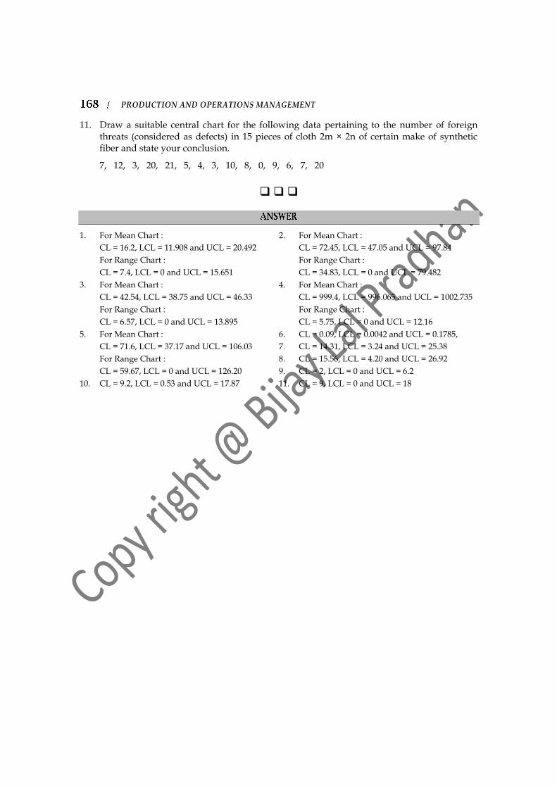
PRODUCTION AND OPERATIONS MANAGEMENT

11. Draw a suitable central chart for the following data pertaining to the number of foreign threats (considered as defects) in 15 pieces of cloth 2m × 2n of certain make of synthetic fiber and state your conclusion.

7, 12, 3, 20, 21, 5, 4, 3, 10, 8, 0, 9, 6, 7, 20

1. For Mean Chart :

CL = 16.2, LCL = 11.908 and UCL = 20.492

For Range Chart :

CL = 7.4, LCL = 0 and UCL = 15.651

2. For Mean Chart :

CL = 72.45, LCL = 47.05 and UCL = 97.84

For Range Chart :

CL = 34.83, LCL = 0 and UCL = 79.482

3. For Mean Chart :

CL = 42.54, LCL = 38.75 and UCL = 46.33

For Range Chart :

CL = 6.57, LCL = 0 and UCL = 13.895

4. For Mean Chart :

CL = 999.4, LCL = 996.065 and UCL = 1002.735

For Range Chart :

CL = 5.75, LCL = 0 and UCL = 12.16

5. For Mean Chart :

CL = 71.6, LCL = 37.17 and UCL = 106.03

For Range Chart :

CL = 59.67, LCL = 0 and UCL = 126.20

6. CL = 0.09, LCL = 0.0042 and UCL = 0.1785,

7. CL = 14.31, LCL = 3.24 and UCL = 25.38

8. CL = 15.56, LCL = 4.20 and UCL = 26.92

9. CL = 2, LCL = 0 and UCL = 6.2

10. CL = 9.2, LCL = 0.53 and UCL = 17.87 11. CL = 9, LCL = 0 and UCL = 18