major tipping points in the earth's climate system and - wwf
TRANSCRIPT

Major Tipping Points in the Earth’s Climate System and Consequences for the
Insurance Sector

The Tipping Points Report was commissioned jointly by Allianz, a leading global financial service provider, and WWF, a leading global environmental NGO.
Contact: WWF (World Wide Fund For Nature) Thomas Duveau, Climate and Finance, WWF Germany Reinhardtstrasse 14, D-10117 Berlin, Germany E-Mail: [email protected], Phone: +49-30-30 87 42 36 Allianz Nicolai Tewes, Corporate Affairs, Allianz SE Koeniginstrasse 28, D-80802 Munich, Germany E-Mail: [email protected], Phone: +49-89-38 00-45 11
Authors: Prof. Tim Lenton, UEA/Tyndall Centre (Tipping points, science, outcomes and research focus) E-Mail: [email protected] Anthony Footitt, UEA/Tyndall Centre (consequence analyses and report production) E-Mail:[email protected] Dr. Andrew Dlugolecki, Andlug Consulting (insurance implications and research focus) E-Mail: [email protected]
Please visit also the online application at: http://knowledge.allianz.com/climate_tipping_points_en.html
Published in November 2009 by WWF - World Wide Fund for Nature (formerly World Wildlife Fund), Gland, Switzerland and Allianz SE, Munich, Germany. Any reproduction in full or in part of this publication must mention the title and credit the above-mentioned publisher as the copyrightowner. © Text (2009) WWF and Allianz SE. All rights reserved.
Andlug Consulting

- iii -
Executive Summary Climate change resulting from emissions of CO2 and other greenhouse gases (GHGs) is widely regarded to be the greatest environmental challenge facing the world today. It also represents one of the greatest social and economic threats facing the planet and the welfare of humankind. The focus of climate change mitigation policy to date has been on "preventing dangerous anthropogenic interference with Earth's climate system". There is no global agreement or scientific consensus for delineating ‘dangerous’ from ‘acceptable’ climate change but limiting global average temperature rise to 2 °C above pre-industrial levels has emerged as a focus for international and national policymakers. The origin and selection of this 2 °C policy threshold is not entirely clear but its determination has been largely informed by assessments of impacts at different levels of temperature increase such as those of the UNFCCC Assessment Report 4 (AR4). With few exceptions, such assessments tend to present a gradual and smooth increase in scale and severity of impacts with increasing temperature. The reality, however, is that climate change is unlikely to be a smooth transition into the future and that there are a number of thresholds along the way that are likely to result in significant step changes in the level of impacts once triggered. The existence of such thresholds or ‘tipping points’ is currently not well reflected in mitigation or adaptation policy and this oversight has profound implications for people and the environment. The phrase ‘tipping point’ captures the intuitive notion that “a small change can make a big difference” for some systems (1). In addition, the term ‘tipping element’ has been introduced to describe those large-scale components of the Earth system that could be forced past a ‘tipping point’ and would then undergo a transition to a quite different state. In its general form, the definition of tipping points may be applied to any time in Earth history (or future) and might apply to a number of candidate tipping elements. However, from the perspective of climate policy and this report we are most concerned with ‘policy-relevant’ tipping elements which might be triggered by human activities in the near future and would lead to significant societal impacts within this century. Considering both the conditions for and likelihood of tipping a number of different elements, the report focuses on the following subset of phenomena and regions where passing tipping points might be expected to cause significant impacts within the first half of this century. Impacts have been explored and assessed in as much detail as possible within such a short study paying particular attention to economic costs and implications for the insurance sector (further information is contained in the main text of the report). Combined sea level rise - global sea level rise (SLR) of up to 2 m by the end of the century combined with localized sea level rise anomaly for the eastern seaboard of North America Exposed assets in Port Megacities - A global sea level rise of 0.5 m by 2050 is estimated to increase the value of assets exposed in all 136 port megacities worldwide by a total of $US 25,158 billion to $US28,213 billion in 2050. This increase is a result of changes in socio-economic factors such as urbanization and also increased exposure of this (greater) population to 1-in-100-year surge events through sea level rise. Exposed assets on NE coast of the US - The impact of an additional 0.15 m of SLR affecting the NE Coast of the US as a result of the localized SLR anomaly means that the following port megacities may experience a total sea level rise of 0.65 m by 2050: Baltimore, Boston, New York, Philadelphia, and Providence. 0.65 m of SLR is estimated to increase asset exposure

- iv -
from a current estimated $US 1,359 billion to $US 7,425 billion. The additional asset exposure from the regional anomaly alone (i.e. 0.65 versus 0.5 m) is approximately $US 298 billion (across the above mentioned cities alone). Insurance aspects - The critical issue is the impact that a hurricane in the New York region would have. Potentially the cost could be 1 trillion dollars at present, rising to over 5 trillion dollars by mid-century. Although much of this would be uninsured, insurers are heavily exposed through hurricane insurance, flood insurance of commercial property, and as investors in real estate and public sector securities. Indian Summer Monsoon - shifts in hydrological systems in Asia as a result of hydrological disturbance of monsoon hydrological regimes (particularly Indian Summer Monsoon) combined with disturbance of fluvial systems fed from the Hindu-Kush-Himalaya-Tibetan glaciers (HKHT) Overview - The impacts on hydrological systems in India under a ‘tipping’ scenario are expected to approximately double the drought frequency (2) and effects from the melting of the Himalayan glaciers and reduced river flow will aggravate impacts. Drought costs - Extrapolating from the 2002 drought using a simple calculation would suggest that the future costs (in today’s prices) might be expected to double from around $US 21 billion to $US 42 billion per decade in the first half of the century. However, a range of other factors are likely to act to increase these costs and consequences in the same period. The most significant of these are likely to be the combined effects of: • decreasing probability of consecutive ‘non-drought’ years from which to accumulate
surpluses (the probability of two consecutive ‘non-drought’ years is halved from 64% to 36% and for three consecutive years reduced from 51% to 22%);
• the pressures of increasing population on food and food surpluses (identified as equal to an increase in production by >40% by 2020 and continuing thereafter); and
• impacts of climate change on irrigation (with up to a 60% reduction in dry season river flows).
The effect of all of the variables is to increase the likelihood, severity and exposure of populations and the economy to potentially devastating conditions within the first half of this century with implications for water resources, health, and food security, and major economic implications not only for India but for economies regionally and worldwide. Insurance aspects - The potential scale of drought losses could abort the initiatives to extend insurance more widely into the rural sector. The wider repercussions of drought through an economic slow-down and deterioration in public finances would impact insurers strongly, through the liquidation of private savings and the impairment of investments in public sector securities. Amazon die-back and drought - committed die-back of the Amazon rainforest and a significant increase in the frequency of drought in western and southern parts of the Amazon basin Amazon die-back - Several model studies have now shown the potential for significant die-back of the Amazon rainforest by late this century and into the next century and that ecosystems can be committed to long-term change long before any response is observable. Any estimate of the cost of Amazon die-back is likely to fall far short of true costs but an
- v -
indication of costs has been derived by application of the UK shadow price of carbon approach (using UK values and approaches). This suggests that • the significant increase in committed die-back that occurs between 1 and 2 °C results in
incremental net present value (NPV) costs of carbon approaching $US 3,000 billion; • policies aimed at stabilization at 2 °C result in NPV costs of the order of $US 3,000 billion
from carbon lost through committed forest die-back (some 1.6 million km2 of Amazon rain forest); and
• beyond ~2 °C the costs of committed die-back rise very rapidly and more than double to around $US 7,800 billion and $US 9,400 billion NPV for 3 °C and 4 °C respectively (with forest area losses of circa 3.9 and 4.3 million km2).
The loss of very substantial areas of forest will result in the release of significant quantities of CO2 and stabilization at 2 °C results in GHG emissions from Amazon die-back equivalent to ~20% of the global historical emissions from global land use change since 1850. This has the potential to interfere very significantly with emissions stabilization trajectories in the latter half of the century and moving forward into the future. Amazon drought - In 2005, large sections of the western Amazon basin experienced severe drought. Recent studies (3) suggest that droughts similar to that of 2005 will increase in frequency from 1-in-20yr to 1-in-2yr and above by between 2025 and 2050 if stabilization at 450 to 550 ppmv CO2e is achieved (with a higher probability if not). The drought of 2005 resulted in a range of impacts including increases in wildfire (with knock-on effects including human health and closure of airports, schools and businesses), interference with navigation (and therefore trade), reductions in agricultural productivity (with knock-on effects to industries servicing agribusinesses and food shortages) and impacts on hydroelectric power generation (which supplies 85% of Brazil’s electricity). These impacts reduced contribution to Brazilian GDP in affected regions including Mato Grosso do Sul, Santa Catarina, Paraná and Rio Grande do Sul. Insurance aspects - Insurers would be directly affected by the economic effects of drought in the region i.e. an economic slow-down, and deterioration in public finances. The impacts on natural forests would be less material, since markets in natural carbon and biodiversity are unlikely to be significant for some time, and the drought risk will become evident during that period. In a broader sense, drought could incentivize investment into other forms of energy, e.g. solar power. Shift in aridity in Southwest North America (SWNA) - a significant shift to a very arid climatology in Southwest North America (SWNA) Overview - Aridity in Southwest North America is predicted to intensify and persist in the future and a transition is probably already underway and will become well established in the coming years to decades, akin to permanent drought conditions (4). Levels of aridity seen in the 1950s multiyear drought or the 1930s Dust Bowl are robustly predicted to become the new climatology by mid-century, resulting in perpetual drought. In California alone this will result in a number of impacts including on water resources, agriculture, and wildfire. Wider impacts - Besides South-western North America, other land regions to be hit hard by subtropical drying include southern Europe, North Africa and the Middle East as well as parts of South America. If the model projections are correct, Mexico in particular faces a future of declining water resources that will have serious consequences for public water supply, agriculture and economic development and this will (and already has) affected the region as a whole, including the United States.

- vi -
Insurance aspects - Insurers are now alert to wildfire risk in the region. The most serious aspects of the tipping point for insurers would therefore be the indirect ones, i.e. economic and labour market disruption and a deterioration of public finances. On the positive side, investment in water management and alternative energy could provide opportunities for fund managers. Take home message Historical GHG emissions have already ‘committed’ us to at least 0.6 °C of further warming. The lack of determined action to reduce GHG emissions means that a warming almost certainly in excess of 2 °C and probably in excess of 3 °C sometime in the latter half of the 21st century is likely unless extremely radical and determined efforts towards deep cuts in emissions are put in place in the short term (by 2015). Alarmingly, this means that, conceivably, there could be tipping elements that have not been triggered yet but which we are already committed to being triggered and/or have already been triggered, but we have yet to fully realize it because of a lag in the response of the relevant system. Although having the potential to affect very significant numbers of people and assets, such elements are virtually absent from policy and decision contexts concerning what changes in temperature or other variables constitute ‘dangerous climate change’. Work to provide early warning of such tipping elements could provide information to facilitate adaptation or mitigation but, at the same time, getting to the point where action is taken on the basis of such early warnings is, arguably, the greater challenge.

- vii -
Contents Executive Summary
1. Introduction 1.1 Current focus of climate policy...............................................................1 1.2 Tipping points...........................................................................................3 1.3 Structure and purpose of the report ......................................................4
2. Policy-relevant tipping elements in the climate system and state of knowledge since IPCC AR4
2.1 Identifying the most policy-relevant tipping elements..........................5 2.2 Tipping elements with impacts revolving around the melting of
ice 2.2.1 Overview..............................................................................................................8 2.2.2 Arctic sea-ice .......................................................................................................8 2.2.3 Sea Level Rise from melting ice sheets and ice caps...........................................9 2.2.4 Greenland Ice Sheet ............................................................................................10 2.2.5 West Antarctic Ice Sheet .....................................................................................11 2.2.6 Continental ice caps.............................................................................................13 2.2.7 Permafrost (and its carbon stores) .......................................................................13 2.2.8 Boreal forest ........................................................................................................14 2.3 Tipping elements that can influence other tipping elements 2.3.1 Overview..............................................................................................................15 2.3.2 Atlantic thermohaline circulation (THC) ................................................................15 2.3.3 El Niño southern oscillation (ENSO).....................................................................17 2.4 Tipping elements involving hydrological regime shifts in the
tropics and expanding sub-tropics 2.4.1 Overview..............................................................................................................18 2.4.2 Amazon rainforest................................................................................................18 2.4.3 West African Monsoon (WAM) and the Sahel ......................................................20 2.4.4 Indian Summer Monsoon (ISM) and other monsoons in South East Asia ............22 2.4.5 South-western North America (SWNA) ................................................................23 2.5 Summary of tipping elements and potential for impacts of
concern on a 50-year time-scale .............................................................25
3. Tipping elements and risks of greatest significance within early 21st century time-scales
3.1 Key impacts of tipping points within 21st century 3.1.1 Identification of key impacts .................................................................................26

- viii -
3.2 Impacts of projected sea level rise associated with tipping elements
3.2.1 Sea level changes and scenario definition ...........................................................26 3.2.2 Estimates of population and assets exposed to global sea level rises of
0.15 and 0.5 m.....................................................................................................27 3.2.3 Impact of NE USA Regional SLR Anomaly ..........................................................33 3.2.4 Insurance and finance implications in NE USA ....................................................34 3.3 Impacts of monsoon interference on India 3.3.1 Hydrological impacts on India under a tipping scenario........................................39 3.3.2 Vulnerability of Indian agriculture and economy ...................................................40 3.3.3 Historical impacts of droughts on Indian agriculture and economy.......................40 3.3.4 Impacts of a tipping scenario ...............................................................................42 3.3.5 Key implications for insurers ................................................................................44 3.4 Hydrological impacts on Amazonia under a tipping scenario
Impacts on Amazonian regions 3.4.1 Overview..............................................................................................................49 3.4.2 Amazon forest die-back .......................................................................................50 3.4.3 Increases in frequency and severity of 2005-like drought conditions....................56 3.4.4 Brazil forest die-back: Insurance and finance implications ...................................60 3.4.5 Issues associated with other aspects of the tipping scenario ...............................62 3.5 Increased aridity in Southwest North America 3.5.1 Overview..............................................................................................................63 3.5.2 Impacts of a shift to a more arid state by reference to historical parallels ............65 3.5.3 Impacts of a shift to a more arid state by reference to existing trends and
projections (SW United States) ...........................................................................65 3.5.4 Regional impacts outside the SW United States ..................................................70 3.5.5 Key implications for insurers of increased aridity in South-western North
America ...............................................................................................................71
4. Summary of impacts and concluding thoughts 4.1 Summary of key impacts and contexts 4.1.1 Overview..............................................................................................................75 4.1.2 Summary of impacts - combined sea level rise ....................................................76 4.1.3 Summary of impacts - Indian Summer Monsoon..................................................76 4.1.4 Summary of impacts - Amazon ............................................................................78 4.1.5 Summary of impacts - Shift in aridity in Southwest North America (SWNA) .........80 4.2 Prospects for early warning and action 4.2.1 Overview..............................................................................................................81 4.2.2 The science of forecasting tipping points .............................................................82 4.2.3 Acting on early warnings ......................................................................................83
5. References

Major Tipping Points in the Earth’s Climate System and Consequences for the Insurance Sector
Page 1
1. Introduction 1.1 Current focus of climate policy Climate change resulting from emissions of CO2 and other greenhouse gases (GHGs) is widely regarded to be the greatest environmental challenge facing the world today. It also represents one of the greatest social and economic threats facing the planet and the welfare of humankind. Political determination of ‘dangerous’ climate change To date, the focus of climate change mitigation policy has been on "preventing dangerous anthropogenic interference with Earth's climate system", where this underlies the United Nations Framework Convention on Climate Change (UNFCCC). Whilst there is no global agreement or scientific consensus for delineating ‘dangerous’ from ‘acceptable’ climate change, limiting global average temperature rise to 2 °C above pre-industrial levels has been emerging as a focus for international and national policymakers. The 2007 Bali conference heard calls for reductions in global greenhouse gas (GHG) emissions to avoid exceeding the 2 °C threshold. In March 2007, the EU reaffirmed its commitment to making its fair contribution to global mean surface temperatures not exceeding 2 °C above pre-industrial levels and the July 2009 G8 summit recognized “the scientific view that the increase in global average temperature above pre-industrial levels ought not to exceed 2 °C”. Thus, the 2 °C threshold has underlined much of the debate on global action to reduce emissions, although the actions required to achieve it are still to be taken. The origin of the 2 °C policy threshold is not entirely clear. Some trace it back to early assessments that the West Antarctic Ice Sheet may have collapsed in past climates that were more than 2 °C warmer. In current assessments, however, it appears related to a combination of factors, including that • estimates suggest that current greenhouse gas concentration is around 430 ppmv
CO2e; • in order to allow policy and implementation some ‘room for manoeuvre’, some
increase in this concentration is regarded by policymakers as inevitable; • stabilization at 450 ppmv CO2e has been reported to provide a mid-value
probability of a global average temperature rise of 2 °C (see for example the Stern Review (5)); and
• set against a background of predicted progressive increases in scale and severity of impacts of increases in global average temperature, a focus for stabilization has become a range between 450 ppmv and 550 ppmv CO2e (see, for example, the Stern Review (5)).
In terms of the potential increases in greenhouse gas concentrations and global average temperature associated with current mitigation policies

Major Tipping Points in the Earth’s Climate System and Consequences for the Insurance Sector
Page 2
• stabilization at 450 ppmv CO2e is actually estimated to provide between a 26%–78% chance of not exceeding 2 °C or, put another way, between 22% and 74% chance of exceeding 2 °C;
• stabilization at 550 ppmv CO2e is estimated to provide between a 63% and 99%
chance of exceeding 2 °C; and • a recent paper concluded that “the current framing of climate change cannot be
reconciled with the rates of mitigation necessary to stabilize at 550 ppmv CO2e and even an optimistic interpretation suggests stabilization much below 650 ppmv CO2e is improbable” (6).
Accordingly, a warming almost certainly in excess of 2°C and probably in excess of 3°C sometime in the latter half of the 21st century therefore seems likely unless extremely radical and determined efforts towards deep cuts in emissions are put in place in the short term (by 2015). In other words, the lack of determined action to reduce GHG emissions means that some degree of climate change is now already inevitable and we are already (or at least very close to being) committed to the ‘dangerous climate change’ associated with the 2°C temperature rise that has been taken as the default threshold. Smooth transition? In terms of impacts, to date climate change mitigation and adaptation policy has been principally guided by assessments such as the Fourth Assessment Report (AR4) of the Intergovernmental Panel on Climate Change (IPCC), as well as many others. Here, much (but not all) of the work tends to present a gradual and smooth increase in scale and severity of impacts with increasing temperature. Whether intentional or unintentional, this tends to project the image that the impact of, say, a global temperature rise slightly in excess of 2°C is somewhat similar to 2°C, only a bit worse. This assumption of a smooth relationship between temperature and level of impact leads policymakers to the assumption that there is an optimal temperature that can be identified by balancing costs of mitigation versus costs of impacts and adaptation. The reality, however, is that climate change is unlikely to be a smooth transition into the future and that there are a number of thresholds along the way that are likely to result in significant step changes in the level of impacts once triggered. For example, although the projections in the IPCC AR4 appear smooth when averaged at the global scale and over relatively long time-scales, in detail they include some striking and sometimes rapid changes at sub-continental scales. Furthermore, since the cut-off for material reviewed in the AR4, the Earth system has displayed some abrupt changes, especially in the Arctic region where the summer sea ice cover has declined precipitously and the Greenland ice sheet has shown accelerating melt. These are just two of many potential examples of large-scale components (or sub-systems) of the Earth system that could undergo a transition to a different state due to human (anthropogenic) interference with the climate (termed climate ‘forcing’) and the interplay of this with natural modes of climate variability.

Major Tipping Points in the Earth’s Climate System and Consequences for the Insurance Sector
Page 3
‘Tipping element’ – a component of the Earth system that can be switched under particular conditions into a qualitatively different state by a small perturbation
‘Tipping point’ - the critical point (in forcing and a feature of the system) at which a transition is triggered for a given ‘tipping element’
The existence of such thresholds is currently not well reflected in mitigation or adaptation policy. This oversight clearly has profound implications for people and the environment. 1.2 Tipping points 1.2.1 Definitions and characteristics Of particular interest and concern in this respect are those transitions where a ‘tipping point’ can be identified at which a relatively small change in climate forcing can commit a system to a qualitative change in state (7).
The phrase ‘tipping point’ captures the intuitive notion that “a small change can make a big difference” for some systems (1). The term ‘tipping element’ has been introduced to describe those large-scale components of the Earth system that could be forced past a ‘tipping point’ and would then undergo a transition to a quite different state.
To formally qualify, tipping elements should satisfy the following conditions (7): • be components of the Earth system that are at least sub-continental in scale
(~1000km); and
• the factors affecting the system can be combined into a single control; and
• there exists a critical value of this control (the tipping point) from which a small perturbation leads to a qualitative change in a crucial feature of the system, after some observation time.
This definition is deliberately broad and inclusive. It includes cases where the transition is faster than the forcing causing it (also known as ‘abrupt’ or ‘rapid’ climate change) and cases where it is slower. It includes transitions that are reversible (where reversing the forcing will cause recovery at the same point it caused collapse) and those that exhibit some irreversibility (where the forcing has to be reduced further to trigger recovery). It also includes transitions that begin immediately after passing the tipping point and those that occur much later (offering a challenge for detection). In some cases, passing the tipping point is barely perceptible but it still makes a qualitative impact in the future. These cases can be thought of as analogous to a train passing the points on a railway track – a small alteration can cause the trajectory of a system to diverge smoothly but significantly from the course it would otherwise have taken1.
1 In the language of physics this is an infinite order phase transition.

Major Tipping Points in the Earth’s Climate System and Consequences for the Insurance Sector
Page 4
1.3 Structure and purpose of the report Section 2 of this report reviews the ‘policy-relevant’ tipping elements in the climate system – those that might be triggered by human activities this century. It begins by summarizing the latest state of knowledge on the tipping elements in the climate system that may be triggered by human activities, where their tipping points may lie, and which forcing agents particularly threaten them. The aim is to identify a subset of the most urgent tipping elements, loosely defined as those that might be triggered soonest and would lead to the greatest and most rapid societal impacts. Considering both the conditions for and likelihood of tipping these elements, Section 3 of the report focuses on a subset of phenomena and regions where passing tipping points might be expected to cause significant impacts within the first half of this century. Impacts are explored and assessed in more detail, with particular reference to economic costs and implications for the insurance sector. In relation to the insurance sector, it is important to bear in mind that the sector comprises two major branches: life (including health and pensions), and non-life (motor, property, liability, etc.; referred to as property/casualty in the USA), backed up by extensive investment of shareholder and policyholder funds. The public sector often plays a direct role as insurer or reinsurer itself, or risks are not insured, so in many cases the private sector is little affected by the direct impact of extreme events or more gradual climatic change. However, the indirect effect through a change on consumer behaviour or deterioration in public finances is likely to be significant. Quantitative information is rarely available on such “knock-on” effects, and resources and time did not permit a formal projection of them, so in general the approach has been to identify the most important linkages and an order of magnitude, if possible. Section 4 summarizes the impacts of tipping scenarios of most concern and, briefly, considers the prospects for early warning of tipping points before we reach them.

Major Tipping Points in the Earth’s Climate System and Consequences for the Insurance Sector
Page 5
2. Policy-relevant tipping elements in the climate system and state of knowledge since IPCC AR4
2.1 Identifying the most policy relevant tipping elements In its general form, the definition of tipping points may be applied to any time in Earth history (or future) and might apply to a number of candidate tipping elements. However, from the perspective of climate policy we are most concerned with those tipping elements which might be triggered by human activities in the near future. Previous work (7) has defined and identified a subset of ‘policy-relevant’ tipping elements where human activities are interfering with the system such that • decisions taken within a “political time horizon” can determine whether a tipping
point is reached; • if the tipping point is reached, a qualitative change in the system would then occur
within an “ethical time horizon”. Any tipping element is integral to the overall functioning of the Earth system and tipping it will have far reaching impacts on physical and ecosystem functioning and the intrinsic ‘value’ of the Earth. However, from an anthropocentric human welfare perspective the list of the most significant tipping elements is likely to be restricted to those affecting a large number of people. Clearly the choices of values for the “political” and “ethical” time horizons are open to debate. Previous work (7) used 100 years for the political time horizon and 1000 years for the ethical time horizon, which to some readers and commentators are rather long. Here we are interested in identifying some of the most urgent tipping elements from an impacts perspective. Hence we introduce an “impacts time horizon” over which significant impacts from passing a tipping point are felt. For the purposes of the present analysis, we restrict more detailed consideration to those tipping phenomena that would lead to significant societal impacts within this century, and where either the lack of sufficient policy engagement in the past and/or decisions taken in the near term have a substantial bearing on whether elements are tipped and impacts are realized. This means that a number of tipping elements are excluded either because their tipping point is inaccessible on the century time-scale, or because passing it would not produce significant impacts on the century time-scale. (However, excluded elements may become a real concern for future policy makers). Based on the above criteria, we have considered the IPCC range of conceivable anthropogenic climate forcing this century where this includes global warming projected to be in the range of 1.1–6.4 °C above the 1980–1999 level by 2100 (8). It is important to note that, even if we could stabilize greenhouse gas concentrations tomorrow (which we cannot), we have already made a ‘commitment’ to at least 0.6 °C of further warming. Alarmingly, this value could be as high as 2 °C if sulphate aerosols currently have a strong climate cooling effect, and it is assumed that their emissions

Major Tipping Points in the Earth’s Climate System and Consequences for the Insurance Sector
Page 6
will continue to decline in an effort to improve air quality (9). This means that, conceivably, there could be tipping elements that • have not been triggered yet but which we are already committed to being triggered;
and/or • have already been triggered, but we have yet to fully realize it because of a lag in
the response of the relevant system. It is also important to note that there are also tipping elements for which the tipping point is not directly related to an increase in GHGs. There are some tipping elements where other anthropogenic forcing factors, notably sulphate and black carbon aerosol emissions, pose a greater threat. Indeed, greenhouse-gas-induced warming may actually protect or strengthen some systems (notably the Indian Summer Monsoon). What are these tipping elements and where are they? Figure 2.1 summarizes on a map some of the potential policy-relevant future tipping elements in the climate system identified and reviewed previously (7). Figure 2.1 – Potential future tipping elements in the climate system, overlain on global
human populations density, as identified by Lenton et al. (2008) (7).
For this report, we have reconsidered the long list of ‘suspects’ and the short list of firm ‘candidates’ for policy-relevant tipping elements in the light of the latest studies. We group the resulting list in terms of the nature of the tipping phenomenon and the associated impacts. This leads to a broad categorisation in terms of the following: • Tipping elements associated with warming and the melting of ice at high latitudes or altitudes, namely:

Major Tipping Points in the Earth’s Climate System and Consequences for the Insurance Sector
Page 7
o the most sensitive systems, which are in the Arctic region and comprise
sea-ice and the Greenland ice sheet; o systems where the key threshold is probably more distant (but with
greater uncertainty) which covers the West Antarctic ice sheet, continental ice caps, permafrost, and the boreal forests.
• Tipping elements that can influence other tipping elements around the world (connecting phenomena), namely:
o the Atlantic thermohaline circulation (THC); and o the El Niño Southern Oscillation (ENSO).
• Tipping elements associated with changes in hydrological systems in the tropics and expanding subtropics, namely:
o the Amazon rainforest; o the West African Monsoon (WAM) and Sahel; o South East Asian monsoons including the Indian Summer Monsoon
(ISM); and o South West North America (SWNA).
The following sub-sections provide an overview of each of these tipping elements following the structure above. In each case a ‘quick facts’ non-technical summary of what each tipping element is, what conditions are required for tipping and what the key concerns/impacts are, is provided in grey boxes. For the reader who wants more detailed information, a technical description of the tipping elements and the evidence is also provided beneath each ‘quick facts’ summary.

Major Tipping Points in the Earth’s Climate System and Consequences for the Insurance Sector
Page 8
2.2 Tipping elements with impacts revolving around the melting of ice 2.2.1 Overview Tipping elements and tipping impacts involving the melting of ice include: • Arctic sea-ice; • Combined Sea Level Rise (SLR) including the melting of:
o Greenland ice sheet (GIS); o West Antarctic Ice sheet (WAIS); and o Continental ice caps;
• Permafrost (and its carbon stores); and • Boreal forest.
2.2.2 Arctic sea-ice Quick facts: Arctic sea-ice
What is it and when/how might it tip? Observed changes in sea ice cover are more rapid than in all IPCC Assessment Report 4 AR4 model projections and the Arctic could already be committed to becoming largely ice-free each summer, within the next few decades. What are the key concerns and impacts?
• Amplified global warming - as Arctic ice melts this exposes a much darker ocean surface, leading to more sunlight being absorbed and hence accelerated ice melt (the ice-albedo feedback).
• Ecosystem change – effects on arctic ecosystems and species including the
iconic polar bear.
Tipping = 0.5–2 °C (above 1980–1999)
Technical details: Arctic sea-ice The Arctic sea-ice can potentially exhibit a tipping point (or points) because as the ice melts this exposes a much darker ocean surface, leading to more sunlight being absorbed and hence accelerated ice melt (the ice-albedo feedback). Whether such a tipping point has already been reached, and how sharp it would be2, are uncertain, but observations clearly show accelerated change is happening. The area coverage of both summer and winter Arctic sea-ice are declining at present, summer sea-ice more markedly, and the ice-pack has thinned significantly. Over 1979–1997, the seasonal minimum area of Arctic sea-ice declined at -4% per decade, but over 1998–2008 it declined at -26% per decade. The area coverage of Arctic sea-ice fell to a record low in September 2007 of 4.2 million km2 (compared to 1980 coverage of 7.8 million km2). Subsequently, in September 2008, the Arctic summer sea-ice reached a record minimum volume (and the area covered was the second lowest on record at 4.5 million km2). The warming due to replacing reflective ice with dark ocean surface (the ice-albedo feedback) has dominated over global warming in causing the thinning and shrinkage of the ice since around 1988. Over 1979–2007, 85% of the
2 In mathematical language: whether there is a bifurcation (in which one state disappears and the system switches inevitably to a different state, with some irreversibility), or just strongly non-linear change.

Major Tipping Points in the Earth’s Climate System and Consequences for the Insurance Sector
Page 9
Arctic region received an increase in solar heat input at the surface, and there is up to a +5% per year trend in some regions (10)3. In the Beaufort Sea, North of Alaska, the annual solar heat input has increased by 3– 4 times, and warming ocean water intruding under the remaining ice pack is now contributing substantially to summer melt. In 2007 and 2008 there was three times greater melt from the bottom of the ice than in earlier years (11). Increased input of warmer ocean water from the Pacific (through the Bering Straits) is part of the problem (12, 13). The patterns of atmospheric (14, 15) and ocean (16) circulation have also contributed to record ice loss by flushing thick, ‘multi-year’ ice out of the basin, reducing the heat capacity of the remaining ice pack and making it more vulnerable to melting. Also, reductions in summertime cloud cover are causing more sunlight to fall on the ice (17). The observed changes in sea ice cover are more rapid than in all IPCC AR4 model projections (despite the observations having been in the mid-range of the models in the 1970s). In half of the models, the summer sea-ice cover disappears during this century (at a polar temperature of around 9 °C above 1980–1999). However, given the observations and further committed warming already ‘in the pipeline’, the Arctic could already be committed to becoming largely ice-free each summer, within the next few decades. Such a transition should be reversible in principle (18), although it would still be difficult to reverse in practice (because anthropogenic forcing would have to be reduced in the region). Recent work has shown that black carbon (soot) from fossil fuel and biomass burning (much of it from South East Asia) has been a major contributor to Arctic regional warming. It is deposited on the sea-ice, darkening it and accelerating melt. A decline in reflective sulphate aerosols in the atmosphere has also contributed significantly to warming, as have the relatively short-lived greenhouse gases ozone and methane. This offers some hope that mitigation of non-CO2 pollutants could help preserve the sea-ice.
2.2.3 Sea Level Rise from melting ice sheets and ice caps The main impact associated with melting of the Greenland Ice Sheet (GIS), West Antarctic Ice Sheets (WAIS) and small continental ice caps, is sea level rise. Hence we begin with a summary of expected combined sea level rise from these sources with further information on the individual components provided below that. Quick facts: Combined Sea Level Rise (SLR) from Greenland and West Antarctic Ice Sheets and continental ice caps Aggregate sea level rise IPCC (2007) chose not to include the uncertain contribution of changing mass of polar ice sheets in their projections of future sea level rise. As such, a ‘No Tipping’ scenario for global SLR from IPCC gives global SLR at around 0.15 m by 2050. There is a convergence on minimum global sea level change being of the order of 75 cm in 2100 and absolute maximum being of the order 2 m. On the basis of this, a ‘Tipping’ Scenario of around 0.5 m of global sea level rise by 2050 is a reasonable starting assumption.
Technical details: Potential sea level rise from melting ice Combining Antarctica, Greenland and small ice caps, the maximum total contribution to sea level rise from melting ice is estimated at ~2 m this century (19). Yet paleo-data from the Eemian interglacial (up to ~2 °C globally warmer than present) indicate that it had peaks of sea level up to 9 m higher than present, and approached them with rates of sea level rise of up to 2.5 m per century (20). Thus, current upper limit estimates of sea level rise of ~2 m this century cannot be ruled out, as they have occurred in a world with temperatures and total ice similar to the present one.
3 Also Donald K. Perovitch, personal communication regarding latest data.

Major Tipping Points in the Earth’s Climate System and Consequences for the Insurance Sector
Page 10
2.2.4 Greenland Ice Sheet Quick facts: Greenland ice sheet (GIS)
What is it and when/how might it tip? The GIS is currently losing mass (i.e. water) at an accelerating rate. It will be committed to irreversible meltdown if the surface mass balance goes negative (i.e. mass of annual snow fall < mass of annual surface melt). Whilst the time-scale for the GIS to melt completely is at least 300 years, because it contains up to 7 m of global sea level rise, its contribution to sea level rise over the whole of this time-scale means that it can still have a significant impact on societies this century. What are the key concerns and impacts?
• Sea level rise - depending on the speed of decay, the GIS could contribute up to 16.5–53.8 cm to global sea level rise this century (19).
• Regionally increased sea level rise - as water added to the ocean takes time
to be globally distributed this leads to sea level rise that is larger than the global average in some regions. Here, the greatest initial sea level rises are predicted down the North Eastern seaboard of the USA (21) affecting a number of US port megacities including Baltimore, Boston, New York, Philadelphia, and Providence.
Tipping = 1–2 °C (above 1980–1999)
Technical details: Greenland ice sheet (GIS) The Greenland ice sheet (GIS) is currently losing mass (i.e. water) at an accelerating rate. This has been linked to a ~2 °C increase in summer temperatures over coastal Southern Greenland since 1990, which correlates with rising Northern Hemisphere temperatures4. From 1996 to 2007 mass loss from the GIS has increased by about a factor of three from ~90Gt yr-1 to ~270Gt yr-1. This is due to both increased surface melt and increased calving of glaciers (particularly into the ocean). In 2007 there was an unprecedented increase in surface melt of the Greenland ice sheet (GIS), mostly south of 70°N and also up the west flank (22), which may be linked to the unprecedented extent of Arctic sea-ice area shrinkage. The melt season was longer with an earlier start, leading to up to 50 days more melt than average. It is part of a longer term trend with an increase in melt extent of 2980 km2 yr-1 (on a daily basis) since the 1970s. Melt-water draining rapidly to the base of the GIS has recently been observed to cause rapid but transient acceleration of ice flow by up to a factor of four (23, 24). Flow is increased over the whole summer season by 50–100% on the western flanks of the ice sheet (25), but no correlation with annual average mass balance has been found (24). Surface melt also modestly accelerates outlet glaciers that flow into the surrounding ocean (by <15%) (25). However, increased flow of these glaciers (by 150–200%) is more strongly related to thinning in their frontal regions causing them to dislodge from the bedrock and accelerate towards the sea. Rapid retreat of one large glacier (Jakobshavn Isbræ) has been dominated by heat input from ocean waters (26). Overall, the surface mass balance of the GIS is still positive (there is more incoming snowfall than melt at the surface, on an annual average), but this is outweighed by the loss of ice due to calving of outlet glaciers. The GIS will be committed to irreversible meltdown if the surface mass balance goes negative. This represents a
4 Prior to 1990, a different phase of the North Atlantic Oscillation meant that regional temperatures were not rising and the GIS was approximately in mass balance, whereas prior to the 1970s temperatures were rising and the GIS was losing mass.

Major Tipping Points in the Earth’s Climate System and Consequences for the Insurance Sector
Page 11
tipping point because as the altitude of the ice sheet surface declines it gets warmer, further accelerating melt (a strong positive feedback). Previous model studies located this threshold at ~3 °C of regional summer warming. The corresponding global warming (accounting for polar amplification of warming) is estimated at ~1–2 °C, although the IPCC AR4 gives a more conservative range of ~1–4 °C. Paleo-data also reveal that the GIS shrunk considerably during the gap between the last two ice ages (called the Eemian interglacial) when regional warming was up to ~4 °C in summer. Most experts in an elicitation give a significant probability of passing the threshold somewhere in the range of 2–4 °C global warming (27)5. However, all existing ice sheet models are now widely acknowledged to be flawed in missing observed rapid decay processes. The time-scale for the GIS to melt is at least 300 years and often given as roughly 1000 years. However, given that it contains up to 7 m of global sea level rise it can still have a significant impact on societies this century. Separate, detailed estimates are that depending on the rapidity of dynamic ice sheet decay, the GIS could contribute up to 16.5–53.8 cm to global sea level rise this century (19). However, the water added to the ocean takes time to be globally distributed, and it causes dynamic responses from the ocean circulation and sea surface height leading to more significant regional sea level rises. In particular, the greatest initial sea level rises are predicted down the North Eastern seaboard of the USA (21).
2.2.5 West Antarctic Ice Sheet
Quick facts: West Antarctic Ice sheet (WAIS)
What is it and when/how might it tip? Recent observations suggest that the WAIS is losing mass and contributing to global sea level rise at a rate that has increased since the early 1990s (7). The WAIS is thought to be less sensitive to warming than the GIS but there is greater uncertainty about this. Unlike GIS, in the case of WAIS it is a warming ocean rather than a warming atmosphere that may be the control that forces the WAIS past a tipping point. Recent expert elicitation gives somewhat higher probabilities of WAIS disintegration under medium (2–4 °C above 1980–1999) and high (>4 °C) global warming than in an earlier survey. What are the key concerns and impacts?
• Sea level rise - a worst case scenario is WAIS collapse within 300 years with a total of ~5 m of global sea level rise (i.e. >1 m per century).
Other recent estimates give the maximum potential contribution of the whole of Antarctica to sea level rise this century as 12.8–61.9 cm (19).
Tipping = 3–5 °C (recent elicitation 2–4 °C) (above 1980–1999)
Technical details: West Antarctic Ice sheet (WAIS) The setting of the West Antarctic Ice Sheet (WAIS) is quite different to Greenland, with most of the bottom of the WAIS grounded below sea level. The WAIS has the potential to collapse if ocean water begins to undercut the ice sheet and separate it from the bedrock, causing the ‘grounding line’ to retreat and triggering further separation (a strong positive feedback). This may be preceded by the disintegration of floating ice shelves and the acceleration of outflow glaciers (ice streams). The West Antarctic Ice Sheet (WAIS) has fairly coherently warmed at >0.1 °C per decade over the past 50 years
5 An alternative model predicts a more distant threshold at ~8°C regional warming (J. Bamber, personal communication).

Major Tipping Points in the Earth’s Climate System and Consequences for the Insurance Sector
Page 12
(28), and observations suggest it is losing mass and contributing to global sea level rise at a rate that has increased since the early 1990s (7). Along the Antarctic Peninsula, strong surface melting has contributed to the collapse of floating ice shelves (29) which in turn has led to accelerated ice discharge from the glaciers behind, which the ice shelves were buttressing. In 2006, ~60 GtC yr-1 were lost from glaciers draining the Antarctic Peninsula, an increase of 145% in 10 years. Further south, glaciers which drain into the Amundsen Sea and Bellingshausen Sea are currently losing ice. In 2006, ~130 GtC yr-1 were lost, an increase of 59% in 10 years. These glaciers drain a region containing ~1.3 m of a total of ~5 m of global sea level rise contained in the WAIS. Overall, mass loss from the WAIS increased 75% in 10 years, whereas snowfall has been roughly constant. The WAIS is thought to be less sensitive to warming than the GIS but there is greater uncertainty about this. At present the GIS is estimated to be losing somewhat more mass (but there is considerable uncertainty in the estimates). Warming ocean water rather than a warming atmosphere may be the control that forces the WAIS past a tipping point under ~3–5 °C warming. For surface melting of the major ice shelves (Ross and Filchner-Ronne) to occur, there would need to be ~5 °C warming of the surface atmosphere in summer. For the main ice sheet at 75–80 °S to reach the freezing point in summer, there would need to be ~8 °C warming of the surface atmosphere. The corresponding global warming depends on the Antarctic polar amplification factor (which varies a lot between models for the 21st century but is likely smaller than that for the Arctic). Recent expert elicitation (27) gives somewhat higher probabilities of WAIS disintegration under medium (2–4 °C above 1980–1999) and high (>4 °C) global warming than in an earlier survey. A worst case scenario is for WAIS collapse to occur within 300 years, with a total of ~5 m of global sea level rise (i.e. >1 m per century). However, other recent estimates give the maximum potential contribution of the whole of Antarctica to sea level rise this century as 12.8–61.9 cm (19).
2.2.6 Continental ice caps Quick facts: Continental ice caps
What are they and when/how might they tip? Smaller continental ice caps are already melting and much of the ice contained in them globally could be lost this century. Such ice caps are generally not considered tipping elements because individually they are too small and there is no identifiable large-scale tipping threshold that results in coherent mass melting. An exception may, however, be glaciers of the Himalayas (the Hindu-Kush-Himalaya-Tibetan glaciers or ‘HKHT’ for short) (9). HKHT glaciers represent the largest mass of ice outside of Antarctica and Greenland. No tipping point threshold has as yet been identified for the region as a whole but IPCC AR4 suggests that much of the HKHT glaciers could melt within this century. What are the key concerns and impacts?
• Reduction in river flow - the HKHT glaciers feed rivers in India, China and elsewhere. A dwindling contribution to river flows will have major implications for populations depending on those rivers and this may be aggravated by other shifts such as in the Indian Summer Monsoon (ISM – see further down). In India alone, melt-water from Himalayan glaciers and snowfields currently supplies up to 85% of the dry season flow and initial modelling suggests that this could be reduced to about 30% of its current contribution over the next 50 years (71).
Tipping = 1–3 °C (above 1980–1999)

Major Tipping Points in the Earth’s Climate System and Consequences for the Insurance Sector
Page 13
2.2.7 Permafrost (and its carbon stores) Quick facts: Permafrost (and its carbon stores)
What is it and when/how might it tip? In simple terms, permafrost is soil and/or subsoil that is permanently frozen throughout the year (and has often been frozen for thousands of years). Observations suggest that permafrost is melting rapidly in some regions, particularly parts of Siberia, and future projections suggest the area of continuous permafrost could be reduced to as little as 1.0 million km2 by the year 2100, which would represent almost total loss (30). An abrupt change in the rate of permafrost shrinkage has been forecast around now, and large areas such as Alaska are projected to undergo the transition from frozen to unfrozen soil in the space of ~50 years (30). Because there is no clear mechanism for a large area to reach a melting threshold nearly simultaneously, melting of most of the world’s permafrost is probably not a tipping element. However, frozen loess (windblown dust) of Eastern Siberia is an exception (31) and could release 2.0–2.8 GtC yr-1 (7.3–10.3 Gt CO2e yr-1) - mostly as CO2 but with some methane - over about a century, removing ~75% of the initial carbon stock. However, to pass this tipping point requires an estimated >9 °C of surface warming, which would only be reached this century under the most extreme scenarios. What are the key concerns and impacts?
• Amplified global warming - In addition to problems of subsidence of structures such as buildings and pipelines, the key concern is that when permafrost melts, the large quantities of carbon it contains are returned back into the atmosphere as methane and carbon dioxide. In addition, frozen compounds called clathrates under the permafrost may be destabilized and result in the release of methane and carbon dioxide.
There have been claims that these responses and the associated release of GHGs will lead to ‘runaway’ global warming as a positive feedback mechanism. These claims are, however, grossly exaggerated and amplification of global temperature change is modest compared to other well known climate feedbacks.
Tipping = >9 °C (Eastern Siberia) (above 1980–1999)

Major Tipping Points in the Earth’s Climate System and Consequences for the Insurance Sector
Page 14
Technical details: Permafrost (and its carbon stores) Continuous permafrost is soil that is frozen all year round. It currently covers ~10.5 million km2 across northern Eurasia, Alaska and Canada. However, permafrost is already melting at an alarming rate in some regions, particularly parts of Siberia which have been a ‘hotspot’ of warming in recent decades. When the Arctic sea-ice declines rapidly, the surrounding Arctic land surface also experiences greatly increased warming (32). This was apparent during August–October 2007, when Western Arctic land temperature was the warmest for the past 30 years (2.3 °C above 1978–2006). A key concern is that when permafrost melts, the carbon it contains is returned back to the atmosphere by microbial activity as methane and carbon dioxide. Also, clathrates under the permafrost may be destabilized and release methane and carbon dioxide to the atmosphere. However, claims that these responses will lead to ‘runaway’ global warming are grossly exaggerated. They do amplify global temperature change but only by a modest amount when compared to other well known climate feedbacks such as increasing atmospheric water vapour (a greenhouse gas). In future projections, the area of continuous permafrost could be reduced to as little as 1.0 million km2 by the year 2100, which would represent almost total loss (30). An abrupt change in the rate of permafrost shrinkage (i.e. a kink in the gradient of area against time) has been forecast around now, and large areas such as Alaska are projected to undergo the transition from frozen to unfrozen soil in the space of ~50 years (30). However, although permafrost melt is a source of concern, most of the world’s permafrost is probably not a tipping element, because there is no clear mechanism for a large area to reach a melting threshold nearly simultaneously (instead, in future projections freezing temperatures are exceeded at different times in different localities (7). One exception has been identified in recent work. The frozen loess (windblown dust) of Eastern Siberia (150–168°E and 63–70°N), also known as Yedoma, is deep (~25 m) and has an extremely high carbon content (2–5%), containing ~500 GtC in total (31). Recent studies have shown the potential for this regional frozen carbon store to undergo self-sustaining collapse, due to an internally-generated source of heat released by biochemical decomposition of the carbon triggering further melting in a runaway positive feedback (33, 34). Once underway, this process could release 2.0–2.8 GtC yr-1 (7.3–10.3 Gt CO2e yr-1) - mostly as CO2 but with some methane - over about a century, removing ~75% of the initial carbon stock. The collapse would be irreversible in the strongest sense that once started, removing the forcing would not stop it continuing. However, to pass the tipping point requires an estimated >9.2 °C of surface warming, which would only be reachable this century under the most extreme scenarios. In all other respects it meets the definition of a tipping element.
2.2.8 Boreal forest Quick facts: Boreal forest
What is it and when/how might it tip? Widespread die-back of the southern edges of boreal forests has been predicted in at least one model when regional temperatures reach around 7 °C above present, corresponding to around 3 °C global warming. What are the key concerns and impacts? • Forest fires, productivity and forest pests & diseases - Under such
circumstances, boreal forest would be replaced by large areas of open woodlands or grasslands that support increased fire frequency.
• Warning signs of ecosystem changes are already apparent in Western Canada
where an infestation of mountain pine beetle has caused widespread tree mortality, and fire frequencies have been increasing (35).
Tipping = 3–5 °C (above 1980–1999)

Major Tipping Points in the Earth’s Climate System and Consequences for the Insurance Sector
Page 15
Technical details: Boreal forest To the south of the continuous permafrost and its tundra vegetation lie the boreal forests. These are predicted to spread north and replace the tundra in future, and shrubby vegetation is already establishing in parts of the tundra. However, the possible tipping point for the boreal forest is closer to its southern edges where widespread die-back has been predicted in at least one model, when regional temperatures reach around 7 °C above present, corresponding to around 3 °C global warming. The causes are complex with warming making the summer too hot for the currently dominant tree species, as well as increased vulnerability to disease, and more frequent fires causing increased mortality, along with decreased reproduction rates. The forest would be replaced over large areas by open woodlands or grasslands that support increased fire frequency. Warning signs are already apparent in Western Canada where an infestation of mountain pine beetle has caused widespread tree mortality, and fire frequencies have been increasing (35).
2.3 Tipping elements that can influence other tipping elements 2.3.1 Overview A feature of the Earth system is that it is just that, a system. This means that all elements are related to all others in some way, whether that relationship appears strong or not. There are, however, a couple of tipping elements exhibiting particularly strong interrelationships with other variables:
• Atlantic thermohaline circulation (THC); and • El Niño southern oscillation (ENSO).
2.3.2 Atlantic thermohaline circulation (THC) Quick facts: Atlantic thermohaline circulation (THC)
What is it and when/how might it tip? Sometimes called the ‘ocean conveyor belt’ the thermohaline circulation (THC) has a profound effect on climate. Collapse of the THC is the archetypal example of a tipping element with the potential tipping point being a shut-off of deep convection and North Atlantic Deep Water (NADW) formation in the Labrador Sea. Best estimates are that reaching the threshold for total THC collapse requires at least 3–5 °C warming within this century. IPCC AR4 views the threshold as more distant and transition of the THC would probably take the order of another 100 years to complete. However, whilst total collapse of the THC may be one of the more distant tipping points, a weakening of the THC this century is robustly predicted by IPCC AR4 models and will have similar (though smaller) effects as a total collapse. What are the key concerns and impacts?
• Complex and combined impacts on other climate variables and tipping elements - THC collapse would tend to cool the North Atlantic and warm the
Tipping = 3–5 °C (above 1980–1999)

Major Tipping Points in the Earth’s Climate System and Consequences for the Insurance Sector
Page 16
Southern Ocean, causing a Southward shift of the Inter-Tropical Convergence Zone (ITCZ) in the atmosphere.
It would raise sea level dynamically by ~1 m in parts of the North Atlantic, including ~0.5 m along the Atlantic coasts of North America and Europe, and reduce sea level in the Southern Ocean.
THC collapse would also have implications for a number of hydrological tipping elements (discussed in Section 2.4).
Technical details: Atlantic thermohaline circulation (THC) The archetypal example of a tipping element is a reorganization of the Atlantic thermohaline circulation (THC) when sufficient freshwater enters the North Atlantic to halt density driven North Atlantic Deep Water (NADW) formation. All models exhibit a collapse of convection under sufficient freshwater forcing, but the additional North Atlantic freshwater input required ranges over 0.1–0.5 Sv (1 Sv = 106 m3s-1). The sensitivity of freshwater input to warming also varies between models, as does whether the transition is reversible or irreversible. Observed freshening of the North Atlantic has contributions from increasing precipitation at high latitudes (which is driving increased Eurasian river input), melting sea-ice, and Greenland ice sheet melt, which currently total ~0.025 Sv. If this is due to the observed ~0.8 °C global warming it could increase several-fold this century. However, best estimates are that reaching the threshold for THC collapse still requires at least 3–5 °C warming within this century. The IPCC AR4 views the threshold as more distant. The transition would probably take the order of another 100 years to complete. A THC collapse would tend to cool the North Atlantic and warm the Southern Ocean, causing a southward shift of the Inter-Tropical Convergence Zone (ITCZ) in the atmosphere. It would also raise sea level dynamically by ~1 m in parts of the North Atlantic, including ~0.5 m along the Atlantic coasts of North America and Europe, and reduce sea level in the Southern Ocean. Although a collapse of the THC may be one of the more distant tipping points, a weakening of the THC this century is robustly predicted by IPCC AR4 models (due to freshening of the North Atlantic by increased precipitation at high latitudes and melting of ice). This in turn will have similar, though smaller, effects as a total collapse. A potential tipping point is a shut-off of deep convection and NADW formation in the Labrador Sea region6 (to the West of Greenland) and a switch to convection only in the Greenland-Iceland-Norwegian Seas (to the East of Greenland), which occurs in some models. This would have dynamic effects on sea level, increasing it down the Eastern seaboard of the USA by around 25 cm in the regions of Boston, New York and Washington DC (in addition to the global steric effect of ocean warming). There will also be implications for a number of hydrological tipping elements discussed below. Rainfall in the tropical and sub-tropical regions on either side of the Atlantic (and further afield) can be strongly influenced by the gradient of sea surface temperatures between the North and South Atlantic (the N-S SST gradient), which is in turn influenced by the underlying strength of the THC. When the THC is strong, this warms the North Atlantic (increasing the N-S SST gradient), whereas when the THC is weak, this cools the North Atlantic (decreasing the N-S SST gradient). The Atlantic THC exhibits natural, internal variability in its strength, which is responsible for an Atlantic multi-decadal oscillation (AMO) in the N-S SST gradient. The AMO was in its positive phase (stronger N-S SST gradient) through the 1930s to the 1950s, it switched to the negative phase in the early 1960s, and switched back to the positive phase around 1995. In the future, switches between phases of the AMO are likely to be overlain on an overall trend towards the negative phase (weaker THC).
6 However, deep convection recently resumed in the Labrador Sea region.

Major Tipping Points in the Earth’s Climate System and Consequences for the Insurance Sector
Page 17
2.3.3 El Niño southern oscillation (ENSO) Quick facts: El Niño southern oscillation (ENSO)
What is it and when/how might it tip? The El Niño southern oscillation (ENSO) is the most significant natural mode of coupled ocean-atmosphere variability in the climate system. Changes in ENSO and a corresponding change in Pacific temperatures occurred around 1976. Prior to 1976 there were low amplitude El Niño events with 2–3 year frequency, subsequently there have been larger amplitude events with 4–5 year frequency. The first coupled model studies predicted a shift from current ENSO variability to more persistent or frequent El Niño conditions. However, in response to a stabilized 3–6 °C warmer climate, the most realistic models simulate increased El Niño amplitude (with no change in frequency). Increase in El Niño amplitude is consistent with the recent observational record. Paleo-data also indicate different ENSO regimes under different climates of the past. What are the key concerns and impacts?
• Complex and combined impacts on other climate variables and tipping elements - higher amplitude El Niño events would have impacts in many regions and on other tipping elements (discussed in Section 2.4).
Tipping = 3–6 °C (above 1980–1999)
Technical details: El Niño southern oscillation (ENSO) The El Niño Southern Oscillation (ENSO) is the most significant natural mode of coupled ocean-atmosphere variability in the climate system. Changes in ENSO and a corresponding change in Pacific temperatures, often described as a ‘regime shift’, occurred around 1976. Prior to 1976 there were low amplitude El Niño events with 2–3 year frequency, subsequently there have been larger amplitude events with 4–5 year frequency. Some attribute aspects of this shift to anthropogenic greenhouse warming. There has been a trend of greater warming in the Western equatorial Pacific than in the Eastern equatorial Pacific over the past century, which has been linked to El Niño events (e.g. in 1983 and 1998) becoming more severe. However, there is no widespread consensus, particularly over changes in ENSO frequency, because the nature of ENSO is still under debate. Some argue that it is a self-sustaining internal oscillation of the climate system, others contend that it is a damped oscillation sustained by external disturbances, and yet others maintain that there is no oscillation and each El Niño event is simply triggered by external (essentially random) disturbances. In the latter two cases, the dependence on stochastic ‘noise’ in the climate system means that any forecasting of El Niño occurrence would always be limited and probabilistic. In future projections, the first coupled model studies predicted a shift from current ENSO variability to more persistent or frequent El Niño conditions. Now that numerous models have been inter-compared, there is no consistent trend in frequency. However, in response to a stabilized 3–6 °C warmer climate, the most realistic models simulate increased El Niño amplitude (with no change in frequency). Furthermore, paleo-data indicate different ENSO regimes under different climates of the past. The mechanisms and time-scale of any transition are unclear but an increase in El Niño amplitude is consistent with the recent observational record. Higher amplitude El Niño events would have impacts in many regions, including ones we explore below.
Major Tipping Points in the Earth’s Climate System and Consequences for the Insurance Sector
Page 18
2.4 Tipping elements involving hydrological regime shifts in the tropics and expanding sub-tropics
2.4.1 Overview A number of tipping elements involve changes in water cycling in the tropics and sub-tropics, with a range of different impacts. The causes are varied and often complex, including interactions with the elements discussed above as well as others. Potential tipping elements include:
• Amazon rainforest; • West African Monsoon (WAM) and the Sahel; • Indian Summer Monsoon (ISM) and other monsoons in South East Asia; and • South Western North America (SWNA).
2.4.2 Amazon rainforest Quick facts: Amazonian rainforest
What is it and when/how might it tip? The Amazon rainforest is well known as a rich cradle of biodiversity. However, it could be threatened by coupled changes in the water cycle and vegetation involving: • An increase in drought anomalies (such as that in 2005), leading to • Amazon rainforest die-back.
The Amazon region is sensitive to changes in both ENSO and the THC, suffering drying during El Niño events, and when the North Atlantic is unusually warm. In 2005, large sections of the western Amazon basin experienced severe drought resulting in significant impacts in a number of regions. The 2005 drought has been linked to an anomalously warm tropical North Atlantic. Recent studies suggest that droughts similar to that of 2005 will increase in frequency in future projections assuming increasing greenhouse gas forcing and decreasing sulphate aerosol (cooling) forcing in the North Atlantic. The 2005 drought was an approximately 1-in-20-yr event, but a 2005-like drought in Amazonia is forecast to become a 1-in-2-yr event by 2025 (at 450 ppmv CO2e) and a 9-in-10-yr event by 2060 (at ~600 ppmv CO2e) with the threshold depending on the rate of increase of CO2 (3). The trees of the Amazon rainforest help maintain rainfall by recycling water to the atmosphere (a positive feedback). They can tolerate short droughts by using their deep roots to access soil water. However, if droughts become more frequent and the dry season continues to get longer, a number of studies have forecast that the forest could reach a threshold beyond which widespread die-back occurs. Potentially up to ~70% of the Amazon rainforest could be lost due to climate change
Tipping = ~10-fold increase in drought frequency at ~2 °C (above pre-industrial) and forest die-back at > ~2 °C

Major Tipping Points in the Earth’s Climate System and Consequences for the Insurance Sector
Page 19
driven die-back by late this century (36). Widespread die-back would occur over a few decades and would be effectively irreversible on any politically meaningful time-scale. The most recent work (37) suggests that the Amazon rainforest could be committed to long-term die-back long before any response is observable, finding, for example, that the risk of significant loss of forest cover in Amazonia rises rapidly for a global mean temperature rise above 2 °C. What are the key concerns and impacts?
• Drought impacts – with effects on wildfire, hydroelectric generation, agricultural production and related service industries, river navigation and livelihoods more generally.
• Die-back impacts – many, including biodiversity loss, decreased rainfall, effect
on livelihoods, and creation of a significant carbon source that amplifies global warming.
Technical details: Effects on Amazonian region One system that is sensitive to changes in both ENSO and the THC is the Amazon rainforest. The Amazon suffers drying during El Niño events, and when the North Atlantic is unusually warm. A severe drought occurred from July to October in 2005 (the dry season) in western and southern parts of the Amazon basin, which led the Brazilian government to declare a state of emergency. Despite ‘greening up’ of large areas of forest (38), the 2005 drought made the Amazon region a significant carbon source, when otherwise it has been a carbon sink (39). The 2005 drought did not have as great an affect in central or eastern Amazonia, a pattern different from the El Niño-related droughts in 1926, 1983, and 1998. Instead, the 2005 drought has been linked to unusually warm sea surface temperatures in the North Atlantic. Reductions in dry season rainfall in Amazonia correlate more broadly with the strength of the Atlantic N-S SST gradient across the equator (3) and hence the underlying strength of the THC. Lengthening of the Amazon dry season is also part of a wider trend in seasonality, associated with weakening of the zonal tropical Pacific atmospheric circulation, which has in turn been linked to anthropogenic greenhouse gas forcing (40). If the trend of a lengthening dry season continues unabated, several model studies have now shown the potential for significant die-back of up to ~70% of the Amazon rainforest by late this century, and its replacement by savannah and caatinga (mixed shrubland and grassland) (36). In the original studies, using predicted climate change from the Hadley Centre model, more persistent El Niño conditions cause die-back of the Amazon rainforest which begins under 3–4 °C global warming. In contrast, weakening of the THC would be expected to help preserve the Amazon by tending to cool the North Atlantic. Expert responses cluster above a probability of 50% for Amazon die-back if global warming exceeds 4 °C (27). However, recent modelling work suggests that the Amazon rainforest may lag climate forcing significantly and hence it may be committed to some die-back long before it is apparent (revealed by allowing the vegetation model to run to equilibrium under a given climate). In the Hadley Centre model, committed die-back begins at 1 °C global warming (above pre-industrial) and by 3 °C, when transient die-back begins, committed die-back has risen to greater than 70% (41). However, other climate models predict different precipitation trends and therefore do not produce die-back (42, 43). Die-back is generally less sensitive to the choice of vegetation model, but the direct effect of CO2 increasing the water use efficiency of vegetation can have a strong effect of tending to shift the die-back threshold further away (P. M. Cox, personal communication). Rainforest loss itself leads to reductions in precipitation, so land-use change could be a trigger, as well as climate change. Thus, linking danger for the Amazon to global warming alone is clearly a limited approach. If the Amazon underwent widespread die-back it could occur over a few decades. Furthermore, model experiments transplanting the die-back vegetation state into a pre-industrial climate show only a very slow rate of recovery over centuries (41), indicating that Amazon die-back could be effectively irreversible on any politically meaningful time-scale.

Major Tipping Points in the Earth’s Climate System and Consequences for the Insurance Sector
Page 20
2.4.3 West African Monsoon (WAM) and the Sahel Quick facts: West African Monsoon (WAM) and the Sahel
What is it and when/how might it tip? The most pronounced hydrological change in the observed climate record was the recent (1960s to 1980s) drought in the Sahel. Key drivers for this were the weakening of the Atlantic North South sea surface temperature (SST) and the weakening of the THC. New results show that more severe, earlier intervals of drought in West Africa were linked to weakening of the THC (44, 45). Recent simulations suggest a tipping point or threshold for THC weakening below which the subsurface North Brazil Current reverses, abrupt warming occurs in the Gulf of Guinea, and the West African Monsoon (WAM) shifts such that it does not seasonally reach the Sahel, and there is an increase in rainfall in the Gulf of Guinea and coastal regions (44). However, in a future simulation with one of the IPCC AR4 models, shift of the WAM unexpectedly leads to wetting and greening of the Sahel and parts of the Sahara back toward conditions last seen around 6000 years ago. Such transitions can potentially occur within years and their reversibility (or irreversibility) is currently unresolved. What are the key concerns and impacts? • Uncertain outcome – there is a recent history of failed efforts to make multi-
decadal forecasts of rainfall in the Sahel. Currently it is unclear whether the Sahel will experience wetting or drying in future. In the best-case scenario, tipping the WAM may provide a net benefit by changing regional atmospheric circulation in a way that wets large parts of the Sahel. .
Tipping = 3–5 °C (above 1980–1999)
Technical details: West African Monsoon (WAM) and the Sahel The most pronounced hydrological change in the observed climate record was the recent (1960s to 1980s) drought in the Sahel. A key driver was weakening of the Atlantic N-S SST gradient, contributed to by both aerosol forcing (46) and weakening of the THC (negative phase of the AMO). Furthermore, new results show that more severe, earlier intervals of drought in West Africa were linked to weakening of the THC (44, 45). This encouraged a phenomenon known as the Atlantic Niño (by analogy with El Niño events in the equatorial Pacific), involving reduced stratification and warming of the Gulf of Guinea. This disrupts the West African Monsoon (WAM), which is usually enhanced by the development of a ‘cold tongue’ in the eastern equatorial Atlantic that increases the temperature contrast between the Gulf of Guinea and the land to the North. The onset of the WAM is linked to a seasonal shift in the trade winds and associated wind-driven currents in the equatorial Atlantic. In a typical year, there is also a northward ‘jump’ of the monsoon into the Sahel in July, which corresponds to a rapid decrease in coastal rainfall and the establishment of the West African Westerly jet in the atmosphere (47). The jump is due to a tipping point in atmospheric dynamics: when the east/west wind changes sharply in the north/south direction, this instability causes the northward perturbation of an air parcel to generate additional northward flow (a strong positive feedback). It is not clear in which direction the WAM might shift in future. The more dangerous option is a southward shift of the WAM, potentially causing further drought in the Sahel. If ocean temperatures change such that the West African Westerly jet fails to form or is weakened below the tipping point needed to create inertial instability, then the rains may fail to move into the continental interior, drying the Sahel. Recent simulations suggest a tipping point or

Major Tipping Points in the Earth’s Climate System and Consequences for the Insurance Sector
Page 21
threshold for THC weakening (~8 Sv), below which the subsurface North Brazil Current reverses, abrupt warming occurs in the Gulf of Guinea (a persistent Atlantic Niño state), and the WAM shifts such that there is a large reduction in rainfall in the Sahel and an increase in the Gulf of Guinea and coastal regions (44). Such an abrupt warming of the Gulf of Guinea and collapse of the WAM is seen in a future simulation with one of the few IPCC AR4 models that produces a realistic present climate in this region (48). Yet unexpectedly this actually leads to wetting and greening of the Sahel and parts of the Sahara back toward conditions last seen around 6000 years ago. A number of model studies have suggested that the regional vegetation-climate system can have two stable states under the present boundary conditions. New work suggests that a strong positive feedback between atmospheric circulation patterns and soil moisture gradients is critical to creating multiple stable states (49). The tipping point between the states (when savannah extends north of 18°N) can be understood in terms of a fundamental reorganization of regional atmospheric dynamics. In the present state, the African easterly jet forms the northern boundary of the WAM circulation, with a Saharan high to the north. In the alternative state, the African easterly jet disappears, moist convection extends into what is now the Sahara, and the West African westerly jet extends much further north, bringing moisture in from the Atlantic. Thus, although the WAM effectively collapses, reducing moisture supply from the south and adversely affecting some regions, there is increased inflow of moist air to the Sahel from the west, wetting it and promoting vegetation growth. The fate of vegetation in the Sahel region will also depend on the degree of land-use change activity (which is currently very high in West Africa). In the best-case scenario the number of people the region can support would increase. Transitions can potentially occur within years and their reversibility (or irreversibility) is currently unresolved.

Major Tipping Points in the Earth’s Climate System and Consequences for the Insurance Sector
Page 22
2.4.4 Indian Summer Monsoon (ISM) and other monsoons in South East Asia Quick facts: Indian Summer Monsoon (ISM) and other monsoons in South East Asia
What is it and when/how might it tip? The arrival of Indian Summer Monsoon (ISM) rainfall is, generally, remarkably reliable, occurring annually in June or July (depending on location). Greenhouse warming would on its own be expected to strengthen the monsoonal circulation, however, the observational record shows declines in ISM rainfall which have been linked to an ‘atmospheric brown cloud’ (ABC) haze created by a mixture of black carbon (soot) and sulphate aerosols. This ABC haze tends to weaken the monsoonal circulation and, in simple models, there is a tipping point for the regional planetary albedo (reflectivity) over the continent which, if exceeded, causes the ISM to collapse altogether. Regional black carbon (soot) emissions from China and India have increased significantly in recent decades. The most pronounced regional hotspot of black carbon emissions is in North Eastern China, which may be linked to a distinct southward shift of monsoonal precipitation in China. What are the key concerns and impacts? • Interference with monsoon cycle and drought frequency - owing to its
reliability, agriculture, livelihoods and economy have grown to depend upon the ISM. Increasing aerosol forcing of the system could weaken the monsoon, but if then removed, greenhouse warming could trigger a stronger monsoon, producing a ‘roller coaster ride’ for many millions of people as, if switches occur, they could happen from one year to the next.
Tipping = Related to aerosol forcing rather than global temperature change
Technical details: Indian Summer Monsoon (ISM) and other monsoons in South East Asia The Indian summer monsoon (ISM) system is already being influenced by aerosol and greenhouse gas forcing. Paleo-records indicate its volatility, with rapid climate changes in the North Atlantic during the last ice age accompanied by flips on and off of monsoonal rainfall. Greenhouse warming, which is stronger over Northern Hemisphere land than the Indian Ocean, would on its own be expected to strengthen the monsoonal circulation. The monsoon is driven by more rapid heating of the land than ocean in summer, causing warm air to rise over the continent, creating a pressure gradient that sucks in moist air from over the ocean. This then rises, the water condenses and rain falls, and there is a return flow of dry air at altitude. However, the observational record shows declines in ISM rainfall, which have been linked to an ‘atmospheric brown cloud’ (ABC) haze created by a mixture of black carbon (soot) and sulphate aerosols. The ABC haze causes more sunlight to be absorbed in the atmosphere and less heating at the surface and it is more concentrated over the continent than the ocean to the south. Hence it tends to weaken the monsoonal circulation. In simple models, there is a tipping point for the regional planetary albedo (reflectivity) over the continent, which if exceeded causes the ISM to collapse altogether. The real picture is likely to be more complex with the potential for switches in the strength and location of the monsoonal rains. Increasing aerosol forcing could further weaken the monsoon, but if then removed, greenhouse warming could trigger a stronger monsoon, producing a ‘roller coaster ride’ for many millions of people. If switches

Major Tipping Points in the Earth’s Climate System and Consequences for the Insurance Sector
Page 23
occur they could happen from one year to the next. Regional black carbon (soot) emissions from China and India have increased significantly in recent decades from a variety of fossil fuel and local biomass burning sources, with detrimental effects on human health as well as on the monsoonal rains. The most pronounced regional hotspot of black carbon emissions is in North Eastern China and there has been a distinct southward shift of monsoonal precipitation in China. This is consistent with the mechanism described for the ISM whereby the formation of an aerosol haze disrupts the monsoonal circulation, potentially shifting it southward in China.
2.4.5 South Western North America (SWNA) Quick facts: Aridity in South Western North America (SWNA)
What is it and when/how might it tip? On decadal and longer time-scales, drought in Western North America (WNA) is linked to periods of increased sea surface temperatures (SSTs) in the North Atlantic, which have been linked to strengthening of the THC (50). Recent drought could also have been contributed to by the removal of aerosol forcing. Aridity in South-western North America (SWNA) is robustly predicted to intensify and persist in future and a transition is probably already underway and will become well established in the coming years to decades, akin to perpetual drought conditions (4). As such, levels of aridity seen in the 1950s multiyear drought or the 1930s Dust Bowl are predicted to become the new climatology by mid-century. Western North America (WNA) has already experienced increased winter air temperature, a declining snow pack (linked to more precipitation falling as rain instead of snow and earlier snow melt), and a shift to earlier run-off (increasing in spring, decreasing in summer), all of which have been attributed to anthropogenic (greenhouse gas and aerosol) forcing (51). Increasing aridity in SWNA may still not qualify formally as a tipping element unless a threshold can be identified. However, evidence suggests that the changes are either imminent or already underway. What are the key concerns and impacts? • Prolonged drought impacts – with impacts on wildfire probability and
consequences for agriculture, water resources and water markets.
Tipping = Predicted imminent/underway
Technical details: Aridity in South Western North America (SWNA) Western North America experienced an interval of severe drought during the Medieval Warm Period (AD 900–1300) (52) and a series of drought intervals more recently, including in the 1930s (“Dust Bowl”), 1950s, and centred on 1999–2002. On decadal and longer time-scales, drought in WNA is linked to periods of increased SSTs in the North Atlantic, which have been linked to strengthening of the THC (positive phase of the AMO) (50). Recent drought could also have been contributed to by the removal of aerosol forcing. There are additional correlations to both positive and negative phases of the Pacific Decadal Oscillation (PDO) (50, 53), and a separate component attributed to observed warming of the Northern Hemisphere (50). Superimposed on this is a shorter-term pattern of

Major Tipping Points in the Earth’s Climate System and Consequences for the Insurance Sector
Page 24
variability, in which drier conditions in the SW and SE US are associated with La Niña conditions in the equatorial Pacific. The “Dust Bowl” drought of the 1930s had an unusual pattern (with maximum drying in the central and northern Great Plains) and recent work has shown that this was due to amplification by land surface feedbacks – crop failure led to reduced soil moisture and soil dust aerosol entering the atmosphere, exacerbating drying in the continental interior (54). During the second half of the twentieth century, the mountainous regions of WNA have experienced increased winter air temperature, a declining snow pack (linked to more precipitation falling as rain instead of snow and earlier snow melt), and a shift to earlier run-off (increasing in spring, decreasing in summer), all of which have been attributed to anthropogenic (greenhouse gas and aerosol) forcing (51). Aridity in South-western North America (SWNA, defined as all land in the region 125–95 °W and 25–40 °N) is robustly predicted to intensify and persist in future and a transition is probably already underway (4). It has been described as a qualitative change to something “…unlike any climate state we have seen in the instrumental record” (4). It still may not qualify as a tipping element unless a threshold can be identified. Increased SWNA aridity has recently been linked to the potential for increased flooding in the Great Plains (55). The key driver is model projected increased summer warming over land (analogous to what drives seasonal monsoons). In future simulations, an increased contrast between the continental low and the North Atlantic sub-tropical high (which extends westwards) strengthens the Great Plains low level jet, which transports moisture from the Caribbean to the Upper Great Plains, triggering flooding there, but starving SWNA of moisture (55).
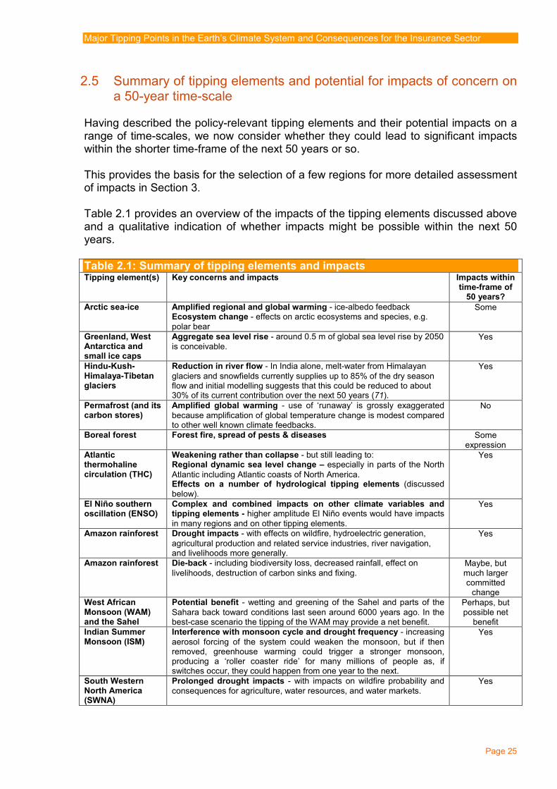
Major Tipping Points in the Earth’s Climate System and Consequences for the Insurance Sector
Page 25
2.5 Summary of tipping elements and potential for impacts of concern on a 50-year time-scale
Having described the policy-relevant tipping elements and their potential impacts on a range of time-scales, we now consider whether they could lead to significant impacts within the shorter time-frame of the next 50 years or so. This provides the basis for the selection of a few regions for more detailed assessment of impacts in Section 3. Table 2.1 provides an overview of the impacts of the tipping elements discussed above and a qualitative indication of whether impacts might be possible within the next 50 years. Table 2.1: Summary of tipping elements and impacts Tipping element(s) Key concerns and impacts Impacts within
time-frame of 50 years?
Arctic sea-ice Amplified regional and global warming - ice-albedo feedback Ecosystem change - effects on arctic ecosystems and species, e.g. polar bear
Some
Greenland, West Antarctica and small ice caps
Aggregate sea level rise - around 0.5 m of global sea level rise by 2050 is conceivable.
Yes
Hindu-Kush-Himalaya-Tibetan glaciers
Reduction in river flow - In India alone, melt-water from Himalayan glaciers and snowfields currently supplies up to 85% of the dry season flow and initial modelling suggests that this could be reduced to about 30% of its current contribution over the next 50 years (71).
Yes
Permafrost (and its carbon stores)
Amplified global warming - use of ‘runaway’ is grossly exaggerated because amplification of global temperature change is modest compared to other well known climate feedbacks.
No
Boreal forest Forest fire, spread of pests & diseases Some expression
Atlantic thermohaline circulation (THC)
Weakening rather than collapse - but still leading to: Regional dynamic sea level change – especially in parts of the North Atlantic including Atlantic coasts of North America. Effects on a number of hydrological tipping elements (discussed below).
Yes
El Niño southern oscillation (ENSO)
Complex and combined impacts on other climate variables and tipping elements - higher amplitude El Niño events would have impacts in many regions and on other tipping elements.
Yes
Amazon rainforest Drought impacts - with effects on wildfire, hydroelectric generation, agricultural production and related service industries, river navigation, and livelihoods more generally.
Yes
Amazon rainforest Die-back - including biodiversity loss, decreased rainfall, effect on livelihoods, destruction of carbon sinks and fixing.
Maybe, but much larger committed
change West African Monsoon (WAM) and the Sahel
Potential benefit - wetting and greening of the Sahel and parts of the Sahara back toward conditions last seen around 6000 years ago. In the best-case scenario the tipping of the WAM may provide a net benefit.
Perhaps, but possible net
benefit Indian Summer Monsoon (ISM)
Interference with monsoon cycle and drought frequency - increasing aerosol forcing of the system could weaken the monsoon, but if then removed, greenhouse warming could trigger a stronger monsoon, producing a ‘roller coaster ride’ for many millions of people as, if switches occur, they could happen from one year to the next.
Yes
South Western North America (SWNA)
Prolonged drought impacts - with impacts on wildfire probability and consequences for agriculture, water resources, and water markets.
Yes

Major Tipping Points in the Earth’s Climate System and Consequences for the Insurance Sector
Page 26
3. Tipping elements and risks of greatest significance within early 21st century time-scales 3.1 Key impacts of tipping points within 21st century 3.1.1 Identification of key impacts Based on the discussion in Section 2, the tipping scenarios most likely to have impacts within (or beginning by) the middle of the 21st century are: • global sea level rise (SLR) of up to 2 m by the end of the century (combined GIS,
WAIS) combined with localized sea level rise anomaly (on top of global SLR) for the eastern seaboard of North America (THC);
• shifts in hydrological systems in Asia as a result of:
o hydrological disturbance of monsoon hydrological regimes particularly Indian Summer Monsoon (from brown cloud forcing and ENSO); and
o disturbance of fluvial systems fed from the Hindu-Kush-Himalaya-Tibetan glaciers (HKHT);
• committed die-back of the Amazon rainforest and a significant increase in the
frequency of the North Atlantic anomaly responsible for the 2005 drought in Western and Southern parts of the Amazon basin; and
• shift to a very arid climatology in South-western North America (SWNA). These impacts are described, assessed, and costed in the following sub-sections. 3.2 Impacts of projected sea level rise associated with tipping elements 3.2.1 Sea level changes and scenario definition One of the potential expected tipping elements that could have significant effects within the first half of this century is that of accelerated global sea level rise (SLR - from a combination of GIS and WAIS) and, in addition, localized sea level rise (on top of global SLR) affecting the NE seaboard of North America (THC). Global Sea Level Rise (SLR) In terms of existing estimates, IPCC (2007) chose not to include the uncertain contribution of changing mass of polar ice sheets in their projections of future sea level rise. As such, a ‘no tipping’ scenario for global SLR from IPCC gives global SLR at around 0.15 m by 2050. Subsequent work by Rahmstorf (56) highlighting an observed empirical correlation between global warming and the rate of sea level rise gives a projected rise by 2100 of 0.5–1.4 m. Recent (as yet unpublished) work (57) by the same author gives increased

Major Tipping Points in the Earth’s Climate System and Consequences for the Insurance Sector
Page 27
projections of sea level rise by 2100 of 0.75–1.9 m. Other, separate, detailed estimates (19) suggest the GIS could contribute up to 16.5–53.8 cm to global SLR this century and WAIS 12.8–61.9 cm with smaller ice caps contributing 17.4–55.1 cm. With thermal expansion of 30 cm the total is 78.5–200.8 cm. This is at least broadly consistent with Rahmstorf’s estimates above – there is a convergence on minimum global sea level change being of the order of 75 cm by 2100 and the absolute maximum being of the order of 2 m. On the basis of this, a ‘tipping’ scenario of around 0.5 m of global SLR by 2050 is a reasonable assumption. NE USA Regional Anomaly Whilst there are other localized regional SLR anomalies, according to the literature the region that could receive the greatest total sea level change is the north-eastern coast of the USA. Yin et al. (58) give ~25 cm by 2050 for the combination of steric (thermal expansion) and dynamic sea level change particularly along the north-eastern coast of the USA. Under low, medium, and high emissions the projected dynamic sea level changes for New York City are 15, 20, and 21 cm respectively by 2100. Accordingly, a regional dynamic sea level change of 0.15 m added to the global SLR of 0.5 m (to give a total of 0.65 m) by 2050 provides a reasonable but higher end estimate for a ‘tipping’ scenario for the NE coast of the USA. Table 3.2.1 summarizes ‘tipping’ and ‘no tipping’ scenarios for SLR. Table 3.2.1: Summary of SLR scenarios NO Tipping Tipping
Global SLR (2050) 0.15 m 0.5 m NE USA Regional SLR (2050) 0.15 m 0.65 m
3.2.2 Estimates of population and assets exposed to global sea level rises of 0.15 and
0.5 m There is broad agreement that sea level rise will displace coastal and delta populations in exposed areas and, as such, population displacement from these areas over time is inevitable. In addition to the slow rise in sea levels, the possibility of coastal flooding events with a return period of 100 or more years presents the possibility of more sudden-onset coastal flooding disasters with impacts on people and assets. There are two key sources of data of most relevance to modelling changes in exposed populations: • estimates of population and land area in a ‘low elevation coastal zone’ (LECZ) (59,
60) defined as the contiguous area along the coast that is less than 10 m above sea level; and
• data produced in the course of the DINAS-COAST (Dynamic and INteractive
Assessment of National, Regional and Global Vulnerability of COASTal Zones to Climate Change and Sea-Level Rise) project.
Major Tipping Points in the Earth’s Climate System and Consequences for the Insurance Sector
Page 28
LECZ data provide an (almost) global picture of populations living in the LECZ but not necessarily exposed to future impacts such as flood risk. The DINAS-COAST data embedded in the DIVA modelling tool (which was the key output of that project) provides an improvement in terms of modelling populations exposed. Data are available on more than 12,000 coastal segments covering the coastline of the globe and the following segment data elements have been combined to produce a model of populations exposed globally (with estimates cross checked with LECZ data for consistency): • land area at different elevations– total area (in km2) at intervals of elevation for
each segment. These are calculated within a zone of 0.2 decimal degrees from the coast (approx 33 km at the equator) and, for deltaic areas, 1.8 decimal degrees (190 km at the equator);
• surge height – 1-in-100-year surge heights (in m) for each segment; • uplift/subsidence – in mm per year for each segment; and • population density – average coastal population density. Estimates of population exposed to global SLR under ‘tipping’ Table 3.2.2 provides data on populations exposed to flood events of 1-in-100-yr frequency at present, with tipping (SLR=0.5 m) versus no tipping (SLR=0.15 m). Data relate to current populations only and do not account for socio-economic changes such as expected population growth by 2050. As such, the numbers exposed provide only an order of magnitude for reference and represent a much lower estimate of actual exposure (in ‘000s) than would be expected. However, the magnitude of the difference between the ‘no tipping’ and ‘tipping’ measured at least as a percentage could be expected to be independent of future population growth (to some extent). Global, regional, and economic area data are provided graphically in Figure 3.2.1 overleaf. In terms of global exposure the ‘tipping’ scenario represents approximately a 38% increase relative to ‘no tipping’ scenarios but distribution of exposure (and therefore impacts) is not even regionally uniform. Here, the estimates suggest that greatest relative change in exposure from tipping is felt in Africa (53% increase) and North America (42%).

Major Tipping Points in the Earth’s Climate System and Consequences for the Insurance Sector
Page 29
-
10,000
20,000
30,000
40,000
50,000
60,000
70,000
80,000
90,000
Africa Asia Europe North America Oceania South America
-
10,000
20,000
30,000
40,000
50,000
60,000
70,000
80,000
90,000
100,000
OECD Non OECD (inc. LDC) LDC
Current Exposure No Tipping Tipping
Populations Exposed to Future 1-in-100-yr Flood Events under Current and Tipping Scenarios (‘000s people exposed)
-
20,000
40,000
60,000
80,000
100,000
120,000
140,000
Global
Distribution of Global Increase in Population Exposure by
Tipping (Versus Not Tipping) 6%
66%
14%
8% 1% 5%
Africa Asia Europe North America Oceania South America
Table 3.2.2: Current and future exposure and increase in exposure to flood events of 1-in-100-yr frequency with tipping (0.5 m) versus no tipping (0.15 m) SLR (current population i.e. not accounting for socio-economic changes such as population growth by 2050) – 1000s people exposed and %
Future Increase in exposure (relative to present) Increase by tipping (versus not tipping) Current
No tip Tip No tip Tip No tip Tip Tip TOTAL 71,341 89,697 123,872 18,356 52,531 26% 74% 34,175 38% Africa 2,801 3,759 5,769 958 2,968 34% 106% 2,009 53% Asia 47,763 60,150 82,679 12,387 34,916 26% 73% 22,529 37% Europe 9,564 11,702 16,422 2,138 6,858 22% 72% 4,720 40% N. America 4,816 6,249 8,879 1,433 4,063 30% 84% 2,630 42% Oceania 1,797 2,262 2,678 465 881 26% 49% 416 18% S. America 4,600 5,574 7,445 974 2,845 21% 62% 1,871 34% OECD 17,581 21,478 29,506 3,897 11,925 22% 68% 8,028 37% Non-OECD 53,761 68,219 94,366 14,458 40,605 27% 76% 26,148 38% LDC 11,738 13,997 18,741 2,259 7,003 19% 60% 4,744 34%
In terms of the magnitude of populations exposed, as noted above, this is sensitive to population growth (and differences between countries and regions). However, as can be seen from the figure, exposure to floods (under all scenarios) is very much higher in Asia than elsewhere and consequently, measured in terms of global distribution of ‘tipping’ impact, global share of increased exposure is very much higher in Asia (66%) than elsewhere (see inset below).
Major Tipping Points in the Earth’s Climate System and Consequences for the Insurance Sector
Page 30
It must be emphasised that exposure does not, however, necessarily translate into impact. Richer countries have (and are more likely to have in the future) better protection levels than those in the developing world. For example, cities such as London, Tokyo, and Amsterdam are protected to better than the 1-in-1000-year standard, while many developing countries have far lower standards, if formal flood defences exist at all (61). Estimation of exposed assets In terms of the economic impact of global SLR, recent work for OECD (61) provides city-scale risks of climate change focusing on the 136 port cities around the world that have more than one million inhabitants. The study estimates changes in exposure to a 1-in-100-year surge-induced flood event (assuming no defences) in the 2070s, assuming SLR of 0.5 m. Unlike the above global analysis of all coastal segments, while focusing on cities, the OECD work considers a range of additional factors such as storm frequency/severity and, most importantly, socio-economic changes such as population growth and urbanization. Estimates of exposed assets are derived from predictions of population exposed and per capita GDP (in $US). In terms of an analysis of the impacts of tipping (with SLR =0.5 m in 2050) there is a need to adjust data from the OECD study downwards to reflect an earlier outcome. For the purposes of this short assessment this has been achieved by isolating data on the increases in exposure from socio-economic changes (such as population growth) by 2075 versus climate change and ‘winding’ estimates back in time to produce an approximation of asset exposure under a tipping scenario of 0.5 m SLR in 2050. Exposed assets in port megacities under a global 0.5 m tipping scenario Adjusting the data from the OECD study downwards provides the estimate that a global sea level rise of 0.5 m by 2050 increases the value of assets exposed in all 136 port megacities by a total of $US 25,158 billion to $US 28,213 billion in 2050. This increase is a result of changes in socio-economic factors such as urbanization and also increased exposure of this (greater) population to 1-in-100-year surge events through sea level rise. The continental distribution and composition of exposed assets in 2050 under this tipping scenario are provided in Figure 3.2.2. This suggests that exposure is highest in Asia followed by North America.

Major Tipping Points in the Earth’s Climate System and Consequences for the Insurance Sector
Page 31
Distribution of Exposed Assets (Tipping - 2050)
$0
$2,000
$4,000
$6,000
$8,000
$10,000
$12,000
$14,000
$16,000
AFRIC
AASIA
AUSTRALA
SIA
EUROPE
N. AM
ERICA
S. AM
ERICA
SE ASIA
$US Billion
Additional exposure by 2050 (socioeconomic)
Additional exposure by 2050 (Climate Change - Tipping)
Current exposure
Top 20 Countries by Size of Exposed Assets (Tipping - 2050)
$0
$1,000
$2,000
$3,000
$4,000
$5,000
$6,000
$7,000
$8,000
$9,000
$10,000
CHINA (I
nc. H
ONG KONG)
UNITED S
TATES O
F AM
ERICA
INDIA
JAPAN
NETHERLA
NDS
THAIL
AND
VIETNAM
BANGLADESH
EGYPT
INDONESIA
UNITED A
RAB EM
IRATE
S
CANADA
UNITED K
INGDOM
BRAZIL
MYANM
AR
REPUBLIC O
F KO
REA
GERMANY
CÔTE D
'IVOIR
E
NIGERIA
AUSTRALI
A
$US Billion
Additional exposure by 2050 (socioeconomic)
Additional exposure by 2050 (Climate Change - Tipping)
Current exposure
Figure 3.2.3 provides further insight into the magnitude of exposed assets by country. The data suggest that nearly 70% (68%) of the global increase in cities’ exposed assets occurs in just three countries (in rank order: China, USA, and India) and 90% in eight countries (China, USA, India, Japan, Netherlands, Thailand, Vietnam, and Bangladesh).
Figure 3.2.2:
Figure 3.2.3:

Major Tipping Points in the Earth’s Climate System and Consequences for the Insurance Sector
Page 32
Top 20 Cities with Highest Increase in Exposed Assets under
Tipping Scenario (US$bn)
$0 $500 $1,000 $1,500 $2,000 $2,500 $3,000
Guangzhou GuangdongMiami
Kolkata (Calcutta)Shanghai
New York-NewarkMumbai (Bombay)
NingboTianjin
Krung Thep (Bangkok)Tokyo
Hong KongOsaka-KobeNew Orleans
RotterdamAmsterdam
DhakaQingdao
Thành-Pho-Ho-Chí-Virginia Beach
Nagoya
Increase in asset exposure ($USBn)
The top 20 port cities with the highest increase in exposed assets under the tipping scenario are provided in Figure 3.2.4.
Figure 3.2.4:
In terms of responses, as noted above, it must be emphasised that exposure does not necessarily translate into impact and the above data do not account for the existence of flood protection measures. As noted in the OECD Port Cities study, in general, cities in richer countries have (and are more likely to have in the future) much better protection levels than those in the developing world. For example, cities like London, Tokyo, and Amsterdam are protected to better than the 1-in-1000-year standard, while many developing countries have far lower standards, if formal flood defences exist at all. There are exceptions to the general relationship between wealth and protection, however. For example, Greater New York, despite having a larger GDP than London, Tokyo, and Amsterdam, is currently only protected to a standard of roughly a 1-in-100-year flood. Shanghai, a developing country city with a lower GDP than New York and European cities, has nevertheless a protection level similar to London. In terms of adopting flood defence strategies in the light of a sea level rise of 0.5 m by 2050, as is noted in the OECD study, putting into place effective disaster management strategies, land use practices and protection investments takes time and previous defence projects (such as the Thames Barrier and the Dutch Delta Project) have shown that implementing coastal protection infrastructure typically has a lead-time of 30 years or more. To achieve adequate protection by 2050, then, this would imply that projects would have to be initiated within the next 10 years (probably much sooner) in order to be timely enough to deliver adequate protection within the time-scale.

Major Tipping Points in the Earth’s Climate System and Consequences for the Insurance Sector
Page 33
3.2.3 Impact of NE USA Regional SLR Anomaly In terms of the impact of the additional 0.15 m of SLR affecting the NE Coast of the USA, of the 17 port megacities in the US considered by the OECD port study, the following might be expected to be affected: • Baltimore; • Boston; • New York; • Philadelphia; • Providence. The resulting increase in asset exposure with the additional 0.15 m (to make 0.65 m in total) has been estimated by calculating the increase in population exposure in the affected coastal sectors from moving from 0.5 m to 0.65 m (based on current population data). The average increase across all coastal sectors is around 13% which, when applied as an uplift to the city scale asset exposures under a 0.5 m scenario (as above) provides some indication of the additional cost of the regional anomaly. The results are provided in Table 3.2.3. The data suggest that the regional anomaly would increase asset exposure from a current estimated $US 1,359 billion to $US 7,425 billion. The additional asset exposure from the regional anomaly alone is approximately $US 298 billion. Table 3.2.3: Asset exposure under NE USA regional SLR anomaly
Agglomeration Current exposure Exposure 2050
(0.5 m) Exposure 2050
(0.65 m) Incremental cost
of anomaly Baltimore $24.3 $26.7 $30.1 $3.5 Boston $76.8 $409.4 $462.6 $53.2 Houston $12.2 $86.0 $86.0 Los Angeles-Long Beach-Santa Ana $16.1 $96.5 $96.5 Miami $416.3 $2,825.9 $2,825.9 New Orleans $233.7 $752.6 $752.6 New York-Newark $320.2 $1,640.5 $1,853.8 $213.3 Philadelphia $32.8 $160.7 $181.6 $20.9 Portland $2.6 $13.3 $13.3 Providence $14.4 $55.5 $62.7 $7.2 San Diego $0.8 $4.1 $4.1 San Francisco-Oakland $24.5 $108.9 $108.9 San Jose $0.9 $8.7 $8.7 Seattle $5.6 $28.4 $28.4 Tampa-St. Petersburg $86.3 $414.1 $414.1 Virginia Beach $84.6 $462.2 $462.2 Washington, D. C. $6.7 $33.5 $33.5 TOTAL $1,358.9 $7,127.0 $7,425.1 $298.1

Major Tipping Points in the Earth’s Climate System and Consequences for the Insurance Sector
Page 34
3.2.4 Insurance and finance implications in NE USA Issues at a glance Event description: Accelerated sea level rise Region: NE America ( in particular). Socio-economic effects: Higher storm damage, erosion, transport disruption. Timing: 2050 onward. Warning: Potentially a strategic surprise in respect of storms. Counter-measures: Sea walls/managed retreat. Type of business
Risks Opportunities
Property Flood & weather damage More demand Casualty Advisory liability. No. Life/health Mainly uninsured. No. Other Interruption/travel/transport More demand Investment/savings Real estate Construction sector.
Major impact Key: Minor impact
Accelerated SLR will compound with a pre-existing, but underestimated, issue in north-east USA, namely storms. In fact the region is vulnerable to summer storms (hurricanes) and also winter storms (61). Previous risk analyses have been disjointed for two main reasons: insurance coverage is split into public (the National Flood Insurance Program mainly for small/medium residential properties), private sector (for storm and commercial flood), with a large element of uninsured properties, particularly for flood. Next, studies have been performed for different purposes: some for SLR, and some for hurricane risk. There is also disagreement on the future hazard profile for hurricanes. This present investigation focuses on New York, because of the high density of assets located there, but as the scientific analysis above shows, the issue affects many other conurbations on the USA eastern seaboard, e.g. Boston. Awareness of flood risk is low at present in the NE USA. Although $US 2,400 billion value (61 per cent) of the property located in New York state is in coastal counties7, the highest penetration of flood coverage of residential properties is just 22% in Bronx County, and for the affected counties of New York State as a whole, coverage is in the region of just five percent. Similar considerations also apply to adjacent states (New Jersey, Massachusetts, Connecticut, and Rhode Island). This low awareness is not just a matter of general ignorance. A major study by the respected Wharton Business School (62) arrived at the remarkably low values for the cost of an extreme storm in the New York area as follows: Return period (years) 100 250 500 Gross cost ($US billion) 2.4 5.8 9.4
This is reflected in the relatively low level of protection in the design of the sea defences, at just 1:100 years for New York, compared to major coastal cities in other developed nations (61). It is worth noting that in fact north-east hurricanes tend to cluster in time, indicating that there is climatic process involved. Data provided by EQE
7 2007 values, per AIR Worldwide Inc.

Major Tipping Points in the Earth’s Climate System and Consequences for the Insurance Sector
Page 35
showed that there were 8 events in the period 1858–96, and 9 between 1953 and 1991 inclusive (63). The loss potential An analysis by AIR Inc. for the Blue Ribbon Commission (64) arrived at a worst case scenario for a Category 4 hurricane in the New York area of a total cost of $US 192 billion (rounded $US 200 billion) on current exposures, of which $US 167 billion would be insured. This is higher than their worst case scenario for a Category 5 hurricane in Florida ($US 178 billion total cost). This is broadly consistent with other estimates. Whereas a repetition of the 1938 Category 3 hurricane “Long Island Express” might cost about $US 30 billion in insured losses according to AIR and Risk Management Solutions, the potential for loss is much higher since the track can vary. Lack of historical events makes it difficult to model such hazards, but it also does appear that once a storm moves north it can in fact intensify through a process called “extratropical transition”. A worst case scenario for a Category 3 hurricane in the New York region is $US 90 billion for insured residential property losses alone according to Kinetic Analysis Corporation, who supplied the estimate for Willis, the international insurance brokers (63). The Blue Ribbon Commission study can therefore serve as the basis for estimating the future cost potential, but already it needs to be modified as follows for several factors to present a more accurate picture of current vulnerability: 1. it ignores non-property classes e.g. auto, marine, and other casualty e.g.
consequential pollution - this could add 10% to the total cost ($US 20 billion), from experience with other hurricanes;
2. it ignores flood damage, since that is covered under the public flood insurance
programme (NFIP) - this could potentially add 50% to the damage ($US 100 billion), from the experience of Hurricane Katrina; and
3. it does not explicitly factor in the consequential disruption to public services, which
is much more important in the built up NY metropolitan centre than in the more diffuse Florida. Given the reliance on underground transportation and services, the impact of flooding would be very serious. Additionally, New York is a national and world business centre, so effects there will be more serious than in, say, Miami. Without detailed study a reliable figure cannot be provided for this but, in the case of New Orleans, some commentators estimated the long-term knock-on costs were twice the size of the property damage (65). That was due to the loss of oil and gas production, but also the prolonged decline in economic and social activity in New Orleans after the storm. In the case of New York, the offshore losses would not be material, but the impact on other branches of the economy would be great. The Blue Ribbon Commission report put the effect at around 0.5% of US GDP, i.e. around $US 300 billion - this might fall disproportionately on the financial sector, since New York is a financial centre. (In contrast to Florida, three-quarters of the real estate at risk in New York is commercial, not residential) Effectively, the consequential losses could double the cost of the storm, after the previous two factors have been included. However, the methodology ignores flood damage,
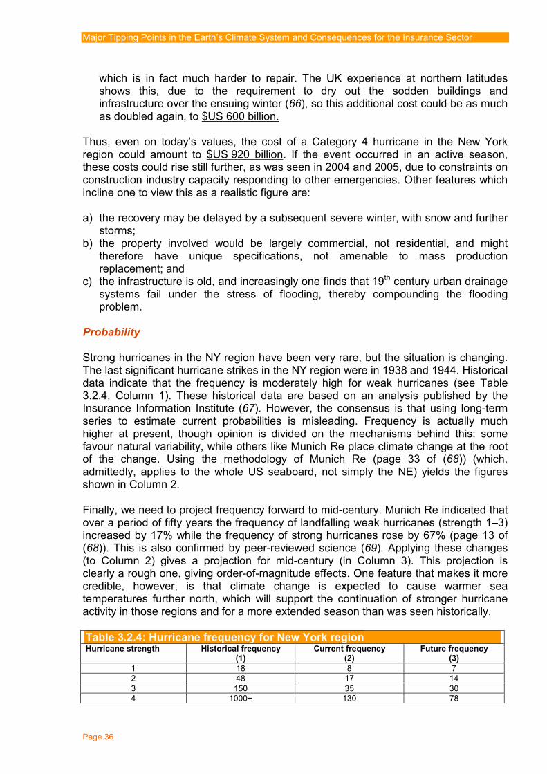
Major Tipping Points in the Earth’s Climate System and Consequences for the Insurance Sector
Page 36
which is in fact much harder to repair. The UK experience at northern latitudes shows this, due to the requirement to dry out the sodden buildings and infrastructure over the ensuing winter (66), so this additional cost could be as much as doubled again, to $US 600 billion.
Thus, even on today’s values, the cost of a Category 4 hurricane in the New York region could amount to $US 920 billion. If the event occurred in an active season, these costs could rise still further, as was seen in 2004 and 2005, due to constraints on construction industry capacity responding to other emergencies. Other features which incline one to view this as a realistic figure are: a) the recovery may be delayed by a subsequent severe winter, with snow and further
storms; b) the property involved would be largely commercial, not residential, and might
therefore have unique specifications, not amenable to mass production replacement; and
c) the infrastructure is old, and increasingly one finds that 19th century urban drainage systems fail under the stress of flooding, thereby compounding the flooding problem.
Probability Strong hurricanes in the NY region have been very rare, but the situation is changing. The last significant hurricane strikes in the NY region were in 1938 and 1944. Historical data indicate that the frequency is moderately high for weak hurricanes (see Table 3.2.4, Column 1). These historical data are based on an analysis published by the Insurance Information Institute (67). However, the consensus is that using long-term series to estimate current probabilities is misleading. Frequency is actually much higher at present, though opinion is divided on the mechanisms behind this: some favour natural variability, while others like Munich Re place climate change at the root of the change. Using the methodology of Munich Re (page 33 of (68)) (which, admittedly, applies to the whole US seaboard, not simply the NE) yields the figures shown in Column 2. Finally, we need to project frequency forward to mid-century. Munich Re indicated that over a period of fifty years the frequency of landfalling weak hurricanes (strength 1–3) increased by 17% while the frequency of strong hurricanes rose by 67% (page 13 of (68)). This is also confirmed by peer-reviewed science (69). Applying these changes (to Column 2) gives a projection for mid-century (in Column 3). This projection is clearly a rough one, giving order-of-magnitude effects. One feature that makes it more credible, however, is that climate change is expected to cause warmer sea temperatures further north, which will support the continuation of stronger hurricane activity in those regions and for a more extended season than was seen historically. Table 3.2.4: Hurricane frequency for New York region Hurricane strength Historical frequency
(1) Current frequency
(2) Future frequency
(3)
1 18 8 7 2 48 17 14 3 150 35 30 4 1000+ 130 78

Major Tipping Points in the Earth’s Climate System and Consequences for the Insurance Sector
Page 37
Compounding effect of higher sea level The calculations have so far ignored the effect of any higher sea level that might be caused by a tipping point (possibly 0.5 metres SLR by mid-century). From the OECD report already cited, the effect of a sea level rise of 0.5 metres would be to increase the exposed assets by a factor of 23% in New York. This would not apply to the wind damage, but to the flood component. Earlier this was estimated to be $US 100 billion at current values, with a further compounding for economic disruption. Keeping this relationship suggests the following costs: Additional effect of SLR = flood damage x increase x grossing up factor for disruption = $US 100 billion x 0.23 x 3 = $US 70 billion (rounded) The aggregate impact on current exposures is therefore: = 920 + 70 = 990 $US billion, or in round terms $US 1 trillion. Future loss potential All of the above figures relate to the asset profile in today’s economy. The OECD Port Cities study made projections of future values in all the major coastal cities of the world, and calculated that for New York, the asset values would be 543% greater than currently, in constant values. If so, then the cost of a strong hurricane in New York would escalate by the same factor, to $US 5.43 trillion. Erosion Apart from repairable damage, increased living and working costs, and loss of production, some land and property will also be permanently lost through erosion. A major study (70) for the US Federal Emergency Management Agency (FEMA) noted that the cost of this is about $US 320 million (at 2000 values) on the Atlantic coastline for the USA, excluding urban centres, which it assumed would be protected. (A breakdown between NE USA and the remainder of the Atlantic coast is not available). This cost is currently borne by the federal NFIP or the real estate owners themselves, not the private insurance market. The historical rate of SLR has been approximately 0.1 m per 50 years. Under this tipping point, an additional 0.5 m would occur within the same period. As an order of magnitude estimate, therefore, this would produce 5 times more additional erosion, giving a cost of approximately $US 2 billion per year. While this is not a direct burden on the private insurance industry, it diverts funds from other sources and, so, indirectly it may create problems for the insurance sector. A further effect that the Heinz Center study noted was that properties expected to be destroyed by erosion begin to lose significant proportions of their value as the perception of future loss strengthens.

Major Tipping Points in the Earth’s Climate System and Consequences for the Insurance Sector
Page 38
Conclusions on Insurance Implications This analysis has uncovered that the tipping point issue for NE USA, though serious, is in fact compounded with another major issue, which is the risk of a major hurricane. New York has been used as the case study to provide a first-order estimate, but in fact the risk extends to several other coastal cities in the region, particularly Boston and Philadelphia. For insurers there are several aspects to consider, including: • The scale of loss potential needs to be reviewed. Typically, insurers assume risk
(sums insured) that is multiples of their resources (net premium and capital). • The volume of claims could be difficult to handle, particularly if they are complex
commercial ones involving water damage and lengthy business interruption. • So far, New York has not been an arena of conflict between insurers and the
regulators, as is the case in Florida. This could change drastically as the hurricane risk becomes apparent.
• The question of economic development in such a hazardous zone has to be
questioned. Investors will expect their assets to be insured, and there could be strong pressure to maintain cover, e.g. for flood damage to commercial property.
• As investors, insurers may have a considerable stake in real estate in New York.
This now needs to be reviewed in terms of the higher risk profile. • Insurers may have significant operations based in the New York region, and need
to review their contingency plans for coping with an emergency, particularly if many other parties are simultaneously affected.

Major Tipping Points in the Earth’s Climate System and Consequences for the Insurance Sector
Page 39
Drought years (observed and predicted)
01234567
1800 - 1809
1810 - 1819
1820 - 1829
1830 - 1839
1840 - 1849
1850 - 1859
1860 - 1869
1870 - 1879
1880 - 1889
1890 - 1899
1900 - 1909
1910 - 1919
1920 - 1929
1930 - 1939
1940 - 1949
1950 - 1959
1960 - 1969
1970 - 1979
1980 - 1989
1990 - 1999
2000s
2010s
2020s
2030s
2040s
Observed drought years (Indian Space Research Organisation - Agricultural and Hydrological droughts)
Observed historical and predicted (in red) drought years (Ramathan et al - based on 1930-1990 hydrological average)
Historical average
Predicted average (2000-2050)
3.3 Impacts of monsoon interference on India 3.3.1 Hydrological impacts on India under a tipping scenario The impacts on hydrological systems in India under a ‘tipping’ scenario are comprised of: • Atmospheric brown cloud forcing – which is predicted to interfere with the Indian
Summer Monsoon (ISM) to approximately double drought frequency (2) from an average of around two per decade (for the period 1800–2000) to four per decade in the first half of this century (see Figure 3.3.1).
• Changes in ENSO amplitude – ENSO is known to cause variation in the Indian
Summer Monsoon. In response to a stabilized 3–6 °C warmer climate, the most realistic models simulate increased El Niño amplitude (with no change in frequency). The mechanisms and time-scale of any transition are unclear but an increase in El Niño amplitude is consistent with the recent observational record and higher amplitude El Niño events will have impacts in many regions, including the ISM.
In addition to the effects of the above on monsoon rainfall, melting of the Himalayan glaciers (HKHT) is expected to reduce river flows. Melt-water from Himalayan glaciers and snowfields currently supplies up to 85% of the dry season flow of the great rivers of the Northern Indian Plain. Initial modelling suggests that this could be reduced to about 30% of its current contribution over the next 50 years with glacial melt (71). This would imply up to a 60% reduction in dry season flow over the next 50 years. Whilst the HKHT is not formally considered a tipping element the impacts on reduced river flows will further aggravate hydrological impacts of interference with monsoon rainfall.
Figure 3.3.1:
Major Tipping Points in the Earth’s Climate System and Consequences for the Insurance Sector
Page 40
3.3.2 Vulnerability of Indian agriculture and economy More than 60% of the cropped area in India still depends solely on the monsoon rainfall that is expected to arrive in June or July (depending on location). The summer, or ‘kharif’, growing season (June–September) coincides with the southwest monsoon and, as such, the monsoon is critical to productivity and success of the kharif crops which account for more than 50% of the food-grain production and more than 65% of the oilseed production in the country (72). The post-monsoon ‘rabi’ growing season (October–November) continues through to the following spring or early summer. The rabi crop is also influenced by the summer monsoon with rainfall towards the end of the monsoon season providing stored soil moisture and some irrigation water for rabi crops. As such, the summer monsoon has considerable influence over both kharif and rabi crop production over India (72). Year-to-year weather variability is the primary cause of year-to-year fluctuations in yield, however cultivated areas are also subject to a broader range of climatic fluctuations. Shortfalls in rainfall can reduce irrigation water supplies, leading to reduced areas under irrigated crops and potentially increased areas under rain-fed crops in the subsequent season. Extreme weather conditions (such as floods, droughts, heat and cold waves, flash floods, cyclones, and hail storms) are also direct hazards to crops and even more subtle fluctuations in weather during critical phases of crop development can have a substantial impact on yields (72). Overall it has been estimated that currently, out of a net sown area of 140 million hectares about 68% is reported to be vulnerable to drought conditions and about 50% of such vulnerable area is classified as ‘severe’, where frequency of drought is almost regular (73). 3.3.3 Historical impacts of droughts on Indian agriculture and economy As can be seen from Figure 3.3.1 drought in India occurs with a frequency of around two per decade. The consequence of these droughts varies but is largely connected with reductions in agricultural production. Table 3.3.1 provides data on the reduction in agricultural production in drought years from the 1970s onwards. The abnormally low rainfall in 1979 in India reduced the overall food-grain by as much as 17% and the 1987 drought in India damaged 58.6 million hectares of cropped area affecting over 285 million people (73). The 1987 Asian drought was one of the worst of the 20th century. Below-normal rainfall and record heat levels damaged crops and stressed livestock throughout South Asia. In India, the main-season grain and oilseed production were reduced to below expected levels and winter crops that depend on residual summer moisture for germination were planted well beyond the normal time. Kharif crop production was down as temperatures and rainfall were respectively among the highest and lowest on record in central and northern rain-fed grain, oilseed, and cotton areas (72). In terms of the rabi (winter) growing season, sowing of wheat (all of which is produced in the winter season) was delayed for months due to insufficient moisture availability for germination. Although most of the wheat crop is irrigated, low reservoir levels and

Major Tipping Points in the Earth’s Climate System and Consequences for the Insurance Sector
Page 41
fuel shortages hampered irrigation efforts. Although the impact of the drought did not approach the severity of the famine years of the 1970s, agricultural imports rose, reserves and exportable supplies were reduced, and growth in other sectors was limited (72). Table 3.3.1: Impacts of drought/poor rainfall years on agricultural production (74) Drought/poor rainfall years
All India rainfall percentage (departure
from normal)
Growth rate Agri. prod. Food-grain prod.
1972-73 (-)24 (-)5.6 (-)7.7 1974-75 (-)12 (-)2.8 (-)4.6 1979-80 (-)19 (-)13.4 (-)16.8 1982-83 (-)14 (-)0.5 (-)2.8 1986-87 (-)13 (-)0.6 (-)4.7 1987-88 (-)19 (-)1.4 (-)2.1 2002-03 (-)19 (-)5.2** (-)18.2** ** calculated from later Ministry of Finance data
Due (primarily) to growth in other sectors of the economy, agriculture’s contribution to India’s GDP has declined (e.g. from around 57% of GDP in 1950–51 to around 28% of GDP in 1998–99) (72). However, agriculture remains the backbone of India’s economy and its economic contribution is much greater than macro-economic indicators suggest. Nearly 70% of the working population depends on agricultural activities for their livelihood and the majority of India’s population depends on cereal and pulse production for sustenance. Agriculture is also a major supplier of raw materials for industry where examples include cotton and jute for textiles, sugar, and vegetable oil. Some 50% of all the income generated in the manufacturing sector in India can be attributed directly or indirectly to agricultural production and agricultural commodities, and products that depend on agriculture account for nearly 70% of the value of exports. Cash crops such as tea, sugar, oilseeds, tobacco, and spices are also major export commodities. As such, owing to both the direct value of agricultural products and agriculture’s indirect impact on employment, rural livelihoods, and other sectors that use agricultural products, the growth of India’s GDP has largely been determined by the trend in agricultural production (72). The most recent (2002) drought reduced the sown area from 124 million hectares in 2001–2002 to 112 million hectares and reduced food-grain production from 212 million tons in 2001–2002 to 174 million tons (73). With the return of more usual rainfall during the 2003 monsoon the economy recovered but the effects on GDP growth can be clearly seen in Figure 3.3.2. Extrapolating from GDP data across the period (74) suggests a drop in expected GDP growth for 2002–03 of around 50.5 thousand Rupees crore (around $US 10.5 billion).

Major Tipping Points in the Earth’s Climate System and Consequences for the Insurance Sector
Page 42
Drop in Indias GDP Growth 2002-03
5%
6%
7%
8%
9%
10%
11%
12%
13%
2000-01 2001-02 2002-03 2003-04
GDP Growth (%) at current prices
Figure 3.3.2:
3.3.4 Impacts of a tipping scenario As noted earlier, under a tipping scenario the average frequency of drought years per decade is expected to increase from around two to four in the first half of this century. Extrapolating from the 2002 drought using a simple calculation would suggest that the future costs (in today’s prices) might be expected to double from around $US 21 billion to $US 42 billion per decade in the first half of the century. However, this is likely to be an underestimate owing to a range of other factors that will influence cost and consequence in the same period. In its 2003 budget and economic report, the Indian Ministry of Finance identifies that the consequences of the 2002 drought (economic and humanitarian) were reduced by the existence of surplus stocks of food-grain accumulated during the three years prior to 2002. In addition, it identifies that the impact of the drought could have been more severe had it not been for the fact that 55% of food-grain is now produced in irrigated areas and 45% in rain-fed areas (against 33% irrigated areas in 1987–88 and 25% in the early 1970s) (74). In terms of future drought scenarios in the first half of this century, however, there are a number of factors that will act to reduce the extent to which surpluses and irrigation are likely to moderate the impacts in future. The most significant of these are likely to be the combined effects of • decreasing probability of consecutive ‘non-drought’ years from which to accumulate
surpluses; • the pressures of increasing population on food and food surpluses; and • impacts of climate change on irrigation.

Major Tipping Points in the Earth’s Climate System and Consequences for the Insurance Sector
Page 43
In terms of the first of these, an increase in drought years produces an accompanying decrease in non-drought years. The probability of non-drought years decreases from 0.8 to 0.6 per year with the result that the probability of two consecutive ‘non-drought’ years to develop a surplus is halved from 64% to 36% and for three consecutive years the probability is reduced by more than half from 51% to 22% (see Table). In both cases the likelihood of consecutive non-drought years is, in future, less than the (40%) probability in any year of a drought. Further reducing the availability of food-grain surplus and magnifying the consequences of drought-year shortages is the pressure of population growth. The population of India is expected to increase to about 1.5 billion by 2030 and food production must increase by five million tons per year to keep pace with this to ensure food security (71). A stepping up of total food-grain production from a current ~212 million metric tons to 300 million metric tons is required by 2020 to meet the food demands of the growing population (73).
This >40% increase in production by 2020 will need to be delivered from both rain-fed agriculture and irrigated production. In terms of the rain-fed agriculture that currently produces ~45% of food-grain, production will clearly be greatly influenced by interference with the summer monsoon. The same, however, is also true of irrigated agriculture which, as noted earlier, was severely affected during the 1987 drought. Whilst it might be assumed that the increase in irrigated area (for example since 1987) will reduce vulnerability and permit greater increases in production, this may be severely limited by hydrological impacts of both monsoon interference and reduced dry season flow in the great rivers of the Northern Indian Plain. Here, melt-water from Himalayan glaciers and snowfields currently supplies up to 85% of the dry season flow8 and initial modelling suggests that this could be reduced to about 30% of its current contribution over the next 50 years (71). This would imply up to a 60% reduction in dry season flow over the next 50 years and, thus, glacial retreat is likely to have major implications for water management and irrigated crop production by 2050. In terms of wheat, for example, the chief wheat-producing states lie along the Indo- Gangetic Plain (Uttar Pradesh, Punjab, Haryana, Madhya Pradesh, Bihar, and Assam) and in the far west (Rajasthan) and account for 95% of the total area under wheat in India. More than 80% of that area under wheat is irrigated (72). Considering all of the impacts and socio-economic changes under a tipping scenario, namely • a doubling of drought frequency, • up to a 60% reduction in dry season river flows, • population growth pressure to increase production by >40% by 2020 (and continue
thereafter), and • Population increase to 1.5 billion by 2050. The effect of all of the variables is to increase the likelihood, severity and exposure of populations and economy to potentially devastating conditions. It can be concluded 8 Note that the glacier-fed rivers are in the west. The Ganges is predominantly rain-fed.
Probability of consecutive ‘non-drought’ years
P Current P Future
P non-drought year 0.8 0.6
2 consecutive non-drought years 0.64 0.36
3 consecutive non-drought years 0.51 0.22

Major Tipping Points in the Earth’s Climate System and Consequences for the Insurance Sector
Page 44
that the elements together provide something of a ‘perfect storm’ within the first half of this century with implications for water resources, health, and food security, as well as major economic implications not only for India but for economies regionally and worldwide. 3.3.5 Key implications for insurers Issues at a glance Event description: Lack of summer precipitation, exacerbated by reduced melt-water from
Tibetan plateau Region: South Asia Socio-economic effects: Harvest failure, industrial interruption. Timing: Progressively, severe by 2050. Warning: Repeated events. Countermeasures: Economic diversification; food imports financed by unaffected industries;
solar power; water efficiency
Type of business
Risks Opportunities
Property No No Casualty No No Life/health Disease, death More demand Other Crop failure, interruption More demand All insurance Slump in demand, fraud No Investment/savings Economic blight in region Water conditioning
Major impact Key: Minor impact
Financial studies of the likely impact of a climate shock on India An extensive review of the economic and financial effects of climate change on the world economy was produced by the IMF in 2008 (75). The study considered mitigation as well as adaptation implications - here we focus on the latter, but it is worth noting that by 2050 IMF projects that there will be 330 million more cars in India - a huge increase in terms of potential emissions, but also in the motor insurance market. The government’s own estimates are that GHG emissions will triple by 2030 from the current level of 1.5 billion tonnes CO2 equivalent per year (76). In India, the literature indicates a large negative impact, due to catastrophic risk (such as a change in the monsoon pattern), with resultant agricultural damages, and deteriorating public health. The cost in Nordhaus is given as 3% of GDP excluding catastrophes, and 5% including catastrophes. IMF performed its own analysis for an un-named nation in South Asia. It found that a climate shock (such as the tipping point under consideration here for example) could lead to a population decline of 2% over the long term. In addition to the population effects, drastic changes in climate could also make many agricultural, distributional, and industrial configurations unviable, forcing the relocation or decommissioning of existing capital stock and the relocation or retraining of labour. Productivity growth would be significantly reduced, and the country’s international competitiveness reduced in existing and new industries. Relative to the baseline, this might ultimately cause more than an 8% contraction in GDP.
Major Tipping Points in the Earth’s Climate System and Consequences for the Insurance Sector
Page 45
For investment, the direct climate-related shocks would add a risk premium shock of one percentage point on capital, as financial markets respond to the country’s deteriorating performance and prospects. Private investment may be hampered by the higher real interest rates. Furthermore, the country would require a large-scale investment in public goods such as relief facilities to protect the population, rebuild infrastructure, and retrain the workforce. The issuance of additional government debt would therefore crowd out private sector investment in other assets. Higher interest rates reduce capital accumulation and therefore GDP, which ultimately ends up 3% lower than in the baseline scenario. The higher risk premium also leads to depreciation of the exchange rate, with a loss of asset value for external investors. Combined therefore, the financial and physical effects of the climate shock could reduce GDP by 10% below ‘business-as-usual’. The financial industry itself is divided on this. A pessimistic view, in line with the IMF paper was given by Morgan Stanley (77). Its global view was that climate change is highly likely to have an impact on the global economy comparable to the collapse of communism and the Internet revolution, but in a negative direction, with stagnation and rising prices due to environmental considerations. Developing countries are more likely to suffer from stagflation since natural disasters and diseases caused by climate change tend to strike countries with poor finances harder. The key instrument of disruption will be “quality and quantity of water.” Morgan Stanley projected that a 2.5 °C rise in global temperature is predicted to cause damage to India of 4.9 per cent of GDP, the highest of any country. This reflects the situation that emerging markets are more vulnerable to climate change because of their geographic exposure, low income levels, poor governance, limited availability of health-care services, less developed financial markets (lending and insurance), and a larger role of climate-sensitive sectors (agriculture, forestry, fishing, and tourism) – particularly agriculture for India. This is borne out by concerns over the 2009 monsoon season. Agriculture still accounts for 18% of India’s GDP (30% in 1990) and 60% of jobs.9 A drought in 2002 caused the agricultural sector to contract by 5.2% in real terms, causing GDP growth to slow from 5.8% to 3.8% over the 2002 fiscal year. In the famous 1979 drought, when the agriculture sector contracted almost 13% in real terms, the economy shrank by more than 5%. It is also worth noting that hydro-power accounts for about 20% of electricity generation. On the other hand, HSBC (78) noted that India is already spending 2.6% of GDP on adaptation to climate vulnerability. Key initiatives include improving arid-land crops, minimising the adverse effects of drought, accelerating afforestation, promoting rain-water harvesting, introducing planning restrictions in coastal areas, introducing proactive disaster management programmes, controlling vector borne diseases such as malaria, and providing crop insurance and credit support for farmers. The authors
9 Economist Intelligence Unit 22 July 2009.

Major Tipping Points in the Earth’s Climate System and Consequences for the Insurance Sector
Page 46
seemed unaware of the potential for climate shocks or the risk of tipping points and were enthusiastic about the investment opportunities in emissions mitigation. In fact the potential for serious regional-scale disruption from climate change is reinforced by the dependence of many millions of people on glacier-fed rivers (see Table 3.3.2). While it is true that, “[t]he glaciers of Nepal do not significantly contribute to the stream flow of the rivers of South Asia at the present time, and there is nothing to indicate that their disappearance would have a major impact on these river systems” (79) , this really only applies to the Ganges and Brahmaputra. Table 3.3.2: Glaciers as a source of water (source: (80)) River Mean discharge
( m3/sec)
Percent of glacier melt in river flow
Population served (millions)
Indus 5533 44.8 178 Ganges 18691 9.1 407 Brahmaputra 19824 12.3 119 Irrawaddy 13565 10.0 (est.)* 33 Salween 1494 8.8 6 Mekong 11048 6.6 57 Yangtze 34000 18.5 369 Yellow 1365 1.3 147 Tarim 423 ** 40.2 8
* Estimated in this report from the values for the rivers to the south and north. ** From Liu et al., 2006 (81)
Discussion Based on the evidence presented in this report, it seems that the financial studies are not pessimistic enough for three reasons: 1. They do not explicitly consider the level of climatic change which is implied by
tipping point conditions identified earlier in the scientific section. 2. They are limited to national focus, but the disruption could be regional, or
coincident with impacts in other geographical regions. 3. They ignore consumer behaviour, particularly in relation to savings. South Asians
buy insurance mainly as a savings product and may realize them in a prolonged crisis (see later).
Climate change and finance in India Where policy is very strong (energy efficiency or renewables) or linked to clear financial gain (Clean Development Mechanism - CDM), business participates quite effectively in climate change-related initiatives. However, general awareness of the impact on ‘business-as-usual’ is low, as the following two pieces of evidence show. In the second Carbon Disclosure Project exercise for India (82) many leading companies (69%) declined to participate, well above the refusal rate in OECD countries. Also, the World Bank carried out a study of how India copes with natural disasters (83).

Major Tipping Points in the Earth’s Climate System and Consequences for the Insurance Sector
Page 47
Essentially, the system was (and still is) a fragmented, post-event public sector one. It lacks a comprehensive catastrophe risk management framework to quantify, analyze, and manage potential losses. The World Bank recommended the development of ex ante funding programmes such as contingency credit and catastrophe reinsurance or bonds because these provide “immediate liquidity that would reduce human suffering, economic loss, and fiscal pressures in the aftermath of a natural disaster, and kick-start economic recovery. Ex ante funding approaches can also foster mitigation and provide incentives for institutional capacity building.” These recommendations have not been adopted. The Indian Insurance Industry Background The Indian insurance market took up 1.32 % of the global insurance market in 2008, and is now the 14th largest national market by premium volume (over $US 56 billion in 2008, and bigger than Russia or Brazil). Prior to 2000, it was a nationalized market, with four government-owned ‘competitors’, but in fact very little innovation and poor levels of service. Since liberalization in 2000, progress has been rapid with increasing numbers of foreign entrants (in partnership with local business). There has been rapid growth in life/savings, health, motor, and fire (84). It is notable that while per capita spending in India is low, compared to other countries, it is heavily weighted towards life (which contains a considerable element of savings). In fact India is much more intensively insured in terms of % GDP devoted to insurance than other countries with higher GDP per capita such as China or Brazil (see Table 3.3.3). The prospects of future growth in the Indian insurance market on a business-as-usual basis are very good. For example, private car ownership is expected to rocket by 2050 (Morgan Stanley; IMF). Other features worth noting are, firstly, the regulations that compel insurers to fulfil a certain fraction of their sales in the rural sector (84). Although this is small, it could be significant if the rural sector is badly affected by climate change. Secondly, the bulk of investments by insurers are mandated in public sector assets. This is seen as a safe haven, and also supportive of government policy, but could become a problem in a crisis. Table 3.3.3: International insurance comparisons (Source Swiss Re. Sigma annual reports on world insurance) Premiums
($US mill., 2008) Real Growth* 1999/2008
Premiums as % GDP (2008)
Premiums per capita ($US, 2008 )
Total 56,190 331% 4.6 47 Life 4.0 41
India
Non-life 0.6 6 Total 140,818 513% 3.3 105
Life 2.2 72 China
Non-life 1.0 33 Total 47,493 174% 3.0 244 Brazil Life 1.4 115

Major Tipping Points in the Earth’s Climate System and Consequences for the Insurance Sector
Page 48
Non-life 1.6 129 Total 243,085 35% 6.6 2,919 Life 3.0 1,347
Germany
Non-life 3.5 1,573 Total 1,240,643 8% 8.7 4,078 Life 4.1 1,901
USA
Non-life 4.6 2,177 Total 4,269,737 27% 7.1 634
Life 4.1 370 World
Non-life 2.9 264 * Based on change in per capita premium expenditure in constant dollar values, to remove demographic effects.
Thirdly, the government is adopting a policy of encouraging weather derivatives as a risk management tool for poor farmers, in the medium of Microinsurance (85). The most recent announcement concerned a scheme developed by MicroEnsure to offer micro-insurance policies for up to 600,000 farmers in 2010 within India's Kolhapur province, allowing them to insure against their rice crops failing due to drought or heavy rains during the crops' flowering period. The policies will be linked with loans from the local Kolhapur District Cooperative Bank (86). The scheme, which is receiving funding from the Bill and Melinda Gates Foundation, will be promoted using comic books to explain how insurance works to farmers who are unfamiliar with insurance. It will also be supported by finance from the Indian government that will effectively halve the price of premiums to around 2.5% of the value of the loan. As well as insuring against crop failure, the scheme also helps farmers to access larger loans to pay for seeds and equipment. Experience shows that banks lend 15 to 40% more to farmers who have insurance. Climate Change Within the Indian insurance industry there is very little realistic planning for a situation where insurance claims may increase with climate change, though in fact the biggest claim to date occurred during the record rainfall in Mumbai in 2005. A government committee was convened but had only one meeting, in May 2003. At present, the focus is on improving penetration of the available insurance products and developing innovative delivery mechanisms to improve the access of the most vulnerable communities, i.e. rural agricultural and slum-dwellers with bundled financial products, through non-specialist agents such as banks, or microfinance institutions (87). It is envisaged that, potentially, climatic problems could be handled through innovative products like weather derivatives and catastrophe bonds (85). Technically this is feasible but it does require better risk analysis which, in turn, requires access to data on the location of insured assets in GIS format, better weather data (a major feature of the weather derivative programme is the installation of hundreds of new weather stations, often privately financed), and new hazard models. However, risks have to fulfil certain conditions to be insurable. One of these is that the price has to be affordable. Under the tipping point scenario, it is predicted that drought frequency will double, to 4 years in 10. At that level, the premium required would be too high, and so the fundamental proposition would collapse. The risk becomes uninsurable. It would be possible for the government to compel insurers to continue the cover, as a condition of offering other lines of business (as happened in Florida with
Major Tipping Points in the Earth’s Climate System and Consequences for the Insurance Sector
Page 49
hurricane insurance), in the expectation that a cross-subsidy would be possible from the larger non-rural segment to the smaller rural one. However, if other lines of business also deteriorate due to the tipping point, this approach is unlikely to succeed. In fact one might even see attempts by different states to break away from a federal system of insurance regulation in order to preserve their own financial system. A second aspect that could arise in a tipping point situation relates to investments and government finance. As noted earlier, much of the Indian insurance market is savings-related, with the bulk of investments in public sector securities. At a time of crisis, consumers will seek to liquidate their savings, even at a financial penalty, to meet emergency needs like higher food prices or relocation. This could result in a glut of government securities on the market, at very low prices, at the very time that the government is seeking to raise new funds to deal with the climatic crisis. Clearly this would result in major funding difficulties, and serious macro-economic risks, such as hyperinflation. A way forward Waiting for this situation to arise is not satisfactory. A more detailed study of the economic and financial implications of this tipping point is urgently required in order to alert policymakers to the issue and convince them of its gravity. At the same time, the insurance industry should campaign for ‘no-regret’ policies. The IMF study noted that climate-aware economic and institutional development is key. Development needs to promote diversification away from heavily exposed sectors and regions, improve access to health, education, and water, and reduce poverty. This requires a change in the policymaking mindset (88). IMF also noted that, “[t]he financial markets’ capacity to reallocate costs and risks to those most willing and able to bear them also will help reduce the social costs of adaptation.” For example, governments should refrain from subsidizing or capping weather insurance premiums, in order to avoid promoting risky behaviour and increasing fiscal risks. In other cases, government investment in flood defences or water conservation may enable insurers to continue providing flood or drought coverage. Another important contribution from the public sector would be to provide reliable and independent data on weather patterns. Technologies for climate change adaptation and companies engaged in that area could therefore become attractive investment propositions. On the broader front, realisation of the tipping point danger could stimulate mitigation activity, which could trigger a phase of faster technological and structural change (77). 3.4 Hydrological impacts on Amazonia under a tipping scenario 3.4.1 Overview The Amazon rainforest is sensitive to changes in both ENSO and the THC and suffers drying during El Niño events and when the North Atlantic is unusually warm. This is expected to result in an increase in both the frequency and severity of drought conditions such as those which occurred in 2005 in Western and Southern parts of the

Major Tipping Points in the Earth’s Climate System and Consequences for the Insurance Sector
Page 50
Amazon basin, and which led the Brazilian government to declare a state of emergency. In addition to increases in drought frequency and severity, several model studies have now shown the potential for significant die-back of the Amazon rainforest by late this century and into the next. Such studies identify that impacts on the Amazon rainforest may lag climate forcing significantly and suggest that, above a threshold of global average temperature rise, significant, unavoidable and effectively irreversible die-back will be committed to long before it becomes apparent. This has very wide implications, both in relations to the future of the Amazon and, owing to release of stored carbon, impacts on a future emissions profile and positive carbon-cycle feedback. 3.4.2 Amazon forest die-back A number of studies (37, 89, 90) have now shown positive feedbacks that reduce the natural uptake of carbon by alterations in ecosystem functioning and, in relation to the Amazon rainforest, forest die-back under climate change. The most recent work (37) suggests that ecosystems can be committed to long-term change long before any response is observable, finding, for example, that the risk of significant loss of forest cover in Amazonia rises rapidly for a global mean temperature rise above 2 °C. Figure 3.4.1 provides data derived from recent work (37) showing a comparison between the realized and committed die-back of mean vegetation cover plotted over time (based on A2 SRES10) and against global mean temperature above pre-industrial. From the figure it can be seen that the changes in forest cover observed at any given point in time, or stabilization (in blue) are significantly less than those that have been committed to (in red). In other words, this means that at any time the forest is showing only a portion of the level of die-back that it will eventually reach because changes in vegetation cover lag behind those of temperature and rainfall. For example, by 2050, when die-back begins to be observed in the simulation, the forest is already committed to eventually losing 50% of its area even without further increases in forcing.
10 SRES – The 2001 IPCC Special Report on Emissions Scenarios presented new emissions scenarios grouped
into families reflecting different mitigation responses, cooperation, responses, behavior, economic growth etc.

Major Tipping Points in the Earth’s Climate System and Consequences for the Insurance Sector
Page 51
Figure 3.4.1: Realized and committed die-back of the Amazon rainforest – after Jones et al. (2009) (37)
Forest Die-back (%)
0%
10%
20%
30%
40%
50%
60%
70%
80%
90%
100%
1 1.5 2 2.5 3 3.5 4 4.5 5
Temperature (Degrees above pre-industrial)
0%
10%
20%
30%
40%
50%
60%
70%
80%
90%
100%
2010 2020 2030 2040 2050 2060 2070 2080 2090 2100 2110
Year (SRES A2 Simulation)
Realised committed
The study suggests that there seems to be a temperature below which the equilibrium state of the forest is approximately constant, but above which the forest cover declines steadily with changing climate. This point could be seen as a threshold beyond which some degree of loss of Amazon forest is inevitable where, beyond this point, there is no sudden transition from `forest' to `no forest' but rather a gradual increase in the level of future committed die-back. In terms of our proximity to such a threshold, it is possible that this tipping element has already been ‘tipped’ and that some degree of committed die-back of the Amazon rainforest is already inevitable. In terms of reaching the 2 °C threshold where there is a significant increase in the area of committed forest die-back, as already noted, current concentrations of GHGs are already at 430 ppmv CO2e and heading towards 450 ppmv CO2e where stabilization even at this concentration is estimated to provide between 22% and 74% chance of exceeding 2 °C. It is worth noting that the concept of committed ecosystem changes applies equally to other biomes and to forest expansion as well as die-back although the response/lag

Major Tipping Points in the Earth’s Climate System and Consequences for the Insurance Sector
Page 52
times and impact on carbon storage might be different. Figure 3.4.2, taken from Jones et al. (2009), shows equivalent results for the boreal forest.
Figure 3.4.2: Dynamic and equilibrium boreal forest extent as it evolves dynamically through the
SRES A2 simulation – taken from Jones et al., 2009 (37).
Implications and headline impacts of committed forest die-back The findings of the Jones et al. (2009) study (37), as well as other related work, highlights a number of serious limitations with any definition of ‘dangerous climate change’ and, in particular, the current political threshold of 2 °C that has underlined much of the debate on global action to reduce emissions. Targets for stabilizing emissions have been based on (largely qualitative) consideration of the impacts of different levels of global warming. However, some aspects of the Earth system continue to respond long after the stabilization implying that stabilization of ‘climate’ does not necessarily mean stabilization of ‘climate change impact’. The impacts of committed (and realized) die-back of the Amazon rainforest stretch well beyond the regional contexts and relate to the ecosystem services provided by the forest. The Amazon rainforest is the world’s largest remaining area of tropical rainforest, supplying services of social, environmental intrinsic and economic value which include (but are far from limited to): • Carbon sequestration and storage - the Amazon covers around 5.3 million km2 and
accounts for around 38% of total tropical biomass. A total of 140 PgC (equivalent to 436,730 million tonnes CO2e) is stored in the biomass of the forest (91).
• Biodiversity - it has been estimated that Brazilian Amazonia houses 20% of the
world’s estimated 1.5 billion species (Capobianco et al., 2001 in (92)). Aside from its intrinsic value, this natural capital stock represents incalculable economic, social and environmental wealth which has not only huge commercial potential but is essential for supporting the livelihoods of forest dwellers and local communities.

Major Tipping Points in the Earth’s Climate System and Consequences for the Insurance Sector
Page 53
• Water cycling - the Amazon River contributes 15–16% of the world’s total river water discharge into the oceans and the forest is a major determinant of water cycling and regional precipitation patterns.
• Intrinsic and economic landscape value - eco-tourism is a fast-expanding field, with
pro-poor eco-tourism gradually establishing itself as a niche market catering for outsiders who wish to spend time living in traditional communities.
Valuation of these assets/ecosystem services is notoriously difficult and, as such, it is difficult to estimate the full impact of the levels of die-back predicted by the Jones et al. study. However, it is possible to derive estimates of what die-back means in terms of area of Amazon rainforest lost and, therein, expected magnitude (and timing) of carbon emissions. On the basis of the latter, it is possible to approximate order of magnitude costs of carbon emissions by applying the shadow price of carbon projected into the future. Area of Forest Loss and Associated Carbon Emissions Figure 3.4.3 provides the Jones et al. estimates of realized and committed die-back converted to area of forest loss (on the left axis) and carbon emissions expressed as millions of tonnes of CO2e (on the right axis). The figure provides these data for both different increments of global temperature increase (above pre-industrial) and the A2 SRES storyline. Following the approach used in Soares et al. (2006) (91), it has been assumed that 85% of the carbon stored in biomass is lost owing to forest die-back.
Figure 3.4.3: Forest Area lost and CO2 emissions
0
1,000,000
2,000,000
3,000,000
4,000,000
5,000,000
6,000,000
2000 2020 2040 2060 2080 2100 2120
Year (SRES A2 Simulation)
Area of Forest Die-back
(Km^2)
0
50,000
100,000
150,000
200,000
250,000
300,000
350,000
400,000
Carbon Dioxide Emissions
(Million t CO2e)

Major Tipping Points in the Earth’s Climate System and Consequences for the Insurance Sector
Page 54
Forest Area Lost and Emissions
0
500,000
1,000,000
1,500,000
2,000,000
2,500,000
3,000,000
3,500,000
4,000,000
4,500,000
5,000,000
0 1 2 3 4 5
Temberature (Degrees above pre-industria l)
Area of Forest Die-back
(Km^2)
0
50,000
100,000
150,000
200,000
250,000
300,000
350,000
Carbon Dioxide
Emissions (Million t CO2e)
To set these emissions in context, it has been estimated that 587 Gt CO2e were emitted to the atmosphere from land use change during the period 1850–2007 and current (net) emissions from land use change for 2006–07 have been estimated at 5.5 Gt CO2e (93). Table 3.4.1 provides a comparison between these values and committed die-back emissions – both total and annual11. From the table, the data suggest that stabilization at, say, 2 °C results in GHG emissions from Amazon die-back equivalent to ~20% of the global historical emissions from land use change since 1850 and annual emissions (post 2050) equivalent to ~20% of the current (2006–07) global net annual emissions from land use change. As such, committed Amazon die-back has the potential to interfere very significantly with emissions stabilization trajectories in the latter half of the century and moving forward into the future. At present, these emissions are not considered as part of assessments to establish global pathways to climate (or climate impact) stabilization. Table 3.4.1: Comparison of total and annual die-back emissions with global emissions from land use change (current and since 1850) Tempera-ture above pre-industrial (°C)
Total committed emissions from Amazon die-back (million t CO2e)
Total committed emissions from
Amazon die-back as a percentage of global emissions from land use
change since 1850
Post 2050 average annual emissions from Amazon die-back (million t CO2e)
Post 2050 average annual emissions from Amazon die-
back as a percentage of global net land use emissions 2006-
7 1 7,424 1% 74 1% 1.5 92,805 16% 928 17% 2 111,366 19% 1,113 20% 2.5 204,171 35% 2,041 37% 3 269,135 46% 2,691 49% 3.5 282,128 48% 2,821 51% 4 300,689 51% 3,007 55% 4.5 322,962 55% 3,230 59%
11 Annual emissions have been derived from committed die-back alone by assuming that committed die-back starts to become realized from 2050 onwards and for a period of 100 years. Emissions have been averaged out over this 100-year timescale.
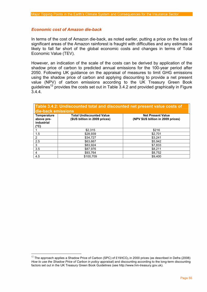
Major Tipping Points in the Earth’s Climate System and Consequences for the Insurance Sector
Page 55
Economic cost of Amazon die-back In terms of the cost of Amazon die-back, as noted earlier, putting a price on the loss of significant areas of the Amazon rainforest is fraught with difficulties and any estimate is likely to fall far short of the global economic costs and changes in terms of Total Economic Value (TEV). However, an indication of the scale of the costs can be derived by application of the shadow price of carbon to predicted annual emissions for the 100-year period after 2050. Following UK guidance on the appraisal of measures to limit GHG emissions using the shadow price of carbon and applying discounting to provide a net present value (NPV) of carbon emissions according to the UK Treasury Green Book guidelines12 provides the costs set out in Table 3.4.2 and provided graphically in Figure 3.4.4. Table 3.4.2: Undiscounted total and discounted net present value costs of die-back emissions Temperature above pre-industrial (°C)
Total Undiscounted Value ($US billion in 2009 prices)
Net Present Value (NPV $US billion in 2009 prices)
1 $2,315 $216 1.5 $28,939 $2,701 2 $34,727 $3,241 2.5 $63,667 $5,942 3 $83,924 $7,833 3.5 $87,976 $8,211 4 $93,764 $8,752 4.5 $100,709 $9,400
12 The approach applies a Shadow Price of Carbon (SPC) of £19/tCO2 in 2000 prices (as described in Defra (2008)
How to use the Shadow Price of Carbon in policy appraisal) and discounting according to the long-term discounting factors set out in the UK Treasury Green Book Guidelines (see http://www.hm-treasury.gov.uk).

Major Tipping Points in the Earth’s Climate System and Consequences for the Insurance Sector
Page 56
Undiscounted value of emissions (based on
shadow price of carbon)
$0
$20,000
$40,000
$60,000
$80,000
$100,000
$120,000
1 1.5 2 2.5 3 3.5 4 4.5
Temperature (Degrees above pre-industrial)
Total value over 150 years (US$ Billions not discounted)
(Discounted) Net Present Value of Emissions
(based on shadow price of carbon)
$0
$1,000
$2,000
$3,000
$4,000
$5,000
$6,000
$7,000
$8,000
$9,000
$10,000
1 1.5 2 2.5 3 3.5 4 4.5
Temperature (Degrees above pre-industrial)
Net Present Value over 150 years (US$ Billions)
Figure 3.4.4: Undiscounted total and discounted net present value costs of die-back emissions
From these figures it can be seen that the significant increase in die-back which occurs between 1 and 2 °C results in incremental NPV costs of carbon approaching $US 3,000 billion and that policies aimed at stabilization at 2 °C result in NPV costs of the order of $US 3,000 billion from carbon lost through die-back of the Amazon alone. Beyond ~2 °C the data suggests costs of committed die-back rise very rapidly and more than double to around $US 7,800 billion and $US 9,400 billion NPV for 3 °C and 4 °C respectively. 3.4.3 Increases in frequency and severity of 2005-like drought conditions In 2005, large sections of the western Amazon basin experienced severe drought resulting in significant impacts in a number of regions. The international section of the 11 December 2005 issue of The New York Times reported that, “[t]he drought has evaporated whole lagoons, and kindled forest fires, killed off fish and crops, stranded boats and the villagers who travel by them, brought disease and wreaked economic havoc.” (94). The drought did not affect central or eastern Amazonia, a pattern different from the El Niño-related droughts in 1926, 1983, and 1998 and the causes of the drought were not related to El Niño but to an anomalously warm tropical North Atlantic. Recent studies (3) investigating the anomaly suggest that droughts similar to that of 2005 will increase in frequency in future projections assuming increasing greenhouse gas forcing and decreasing sulphate aerosol (cooling) forcing in the North Atlantic. Figure 3.4.5 taken from Cox et al. (3) shows predicted change in the probability of a 2005-like drought in Amazonia. The authors identify that 2005 was an approximately 1-

Major Tipping Points in the Earth’s Climate System and Consequences for the Insurance Sector
Page 57
in-20-yr event, but will become a 1-in-2-yr event by 2025 (at 450 ppmv CO2e) and a 9-in-10-yr event by 2060 (at ~600 ppmv CO2e) with the threshold obviously depending on the rate of increase of CO2. Figure 3.4.5: Predicted change in the probability of a 2005-like drought in Amazonia, based on
results from the HadCM3LC GCM run with aerosols13 (after Cox et al., 2008 (3))
At present global mitigation policy focus is towards 2 °C as the threshold for ‘dangerous climate change’ but progress towards a stabilization pathway to deliver the 450 ppmv CO2e that is predicted to provide a 26%–78% chance of not exceeding 2 °C is slow and 550 ppmv CO2e may subsequently become the focus of global mitigation efforts (with between a 63% and 99% chance of exceeding 2 °C). Given that the threshold for tipping increases in 2005-like drought conditions is already likely to have been exceeded, this means that expected frequency of 2005-like drought conditions increases from the current 5% (1 in 20 years) to 50% (1 in 2 years) by 2025 and 67% (>1 in 2 years) by 2050 if stabilization between 450 and 550 ppmv CO2e is achieved. Impact of increases in 2005-like drought frequency Clearly, when considering the impacts of increases in 2005-like drought conditions, the first point reference for assessing impacts is the 2005 drought itself. Interestingly, while the Cox et al. (2008) data (3) suggest a current frequency for 2005-like conditions of 1 in 20 years, the literature on the 2005 drought suggests that 2005 was the most severe drought in the past 40 years and one of the most intense of the last hundred years. Logically this suggests either that escalation of 2005-like conditions to 2005-like drought impacts does not always occur (i.e. 2005-like conditions are not always manifested as severe drought) or that the current GHG concentration of ~430 ppmv CO2e has already ‘tipped’ the anomaly. Examination of Figure 3.4.5 (b) would strongly suggest the latter.
13 Probabilities are calculated as the fraction of years that exceed the July–October 2005 anomaly in the ANSG index, using the 20-yr window centred on each year: a, probability versus year; b, probability versus simulated CO2 concentration. The dotted lines respectively mark the points beyond which the 2005 anomaly is exceeded in 50% of the simulated years (2025, 450 p.p.m.v. of CO2) and in 90% of the simulated years (2060, 610 p.p.m.v. of CO2).
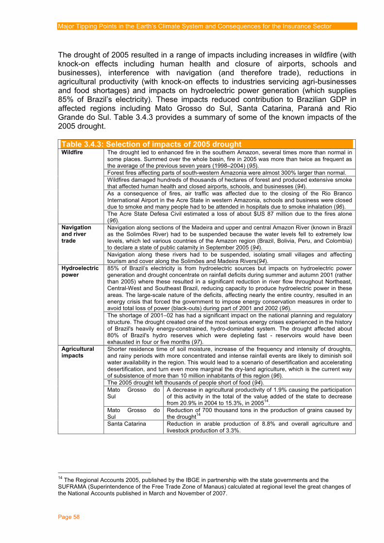
Major Tipping Points in the Earth’s Climate System and Consequences for the Insurance Sector
Page 58
The drought of 2005 resulted in a range of impacts including increases in wildfire (with knock-on effects including human health and closure of airports, schools and businesses), interference with navigation (and therefore trade), reductions in agricultural productivity (with knock-on effects to industries servicing agri-businesses and food shortages) and impacts on hydroelectric power generation (which supplies 85% of Brazil’s electricity). These impacts reduced contribution to Brazilian GDP in affected regions including Mato Grosso do Sul, Santa Catarina, Paraná and Rio Grande do Sul. Table 3.4.3 provides a summary of some of the known impacts of the 2005 drought. Table 3.4.3: Selection of impacts of 2005 drought
The drought led to enhanced fire in the southern Amazon, several times more than normal in some places. Summed over the whole basin, fire in 2005 was more than twice as frequent as the average of the previous seven years (1998–2004) (95). Forest fires affecting parts of south-western Amazonia were almost 300% larger than normal. Wildfires damaged hundreds of thousands of hectares of forest and produced extensive smoke that affected human health and closed airports, schools, and businesses (94). As a consequence of fires, air traffic was affected due to the closing of the Rio Branco International Airport in the Acre State in western Amazonia, schools and business were closed due to smoke and many people had to be attended in hospitals due to smoke inhalation (96).
Wildfire
The Acre State Defesa Civil estimated a loss of about $US 87 million due to the fires alone (96). Navigation along sections of the Madeira and upper and central Amazon River (known in Brazil as the Solimões River) had to be suspended because the water levels fell to extremely low levels, which led various countries of the Amazon region (Brazil, Bolivia, Peru, and Colombia) to declare a state of public calamity in September 2005 (94).
Navigation and river trade
Navigation along these rivers had to be suspended, isolating small villages and affecting tourism and cover along the Solimões and Madeira Rivers(94). 85% of Brazil’s electricity is from hydroelectric sources but impacts on hydroelectric power generation and drought concentrate on rainfall deficits during summer and autumn 2001 (rather than 2005) where these resulted in a significant reduction in river flow throughout Northeast, Central-West and Southeast Brazil, reducing capacity to produce hydroelectric power in these areas. The large-scale nature of the deficits, affecting nearly the entire country, resulted in an energy crisis that forced the government to impose energy conservation measures in order to avoid total loss of power (black-outs) during part of 2001 and 2002 (96).
Hydroelectric power
The shortage of 2001–02 has had a significant impact on the national planning and regulatory structure. The drought created one of the most serious energy crises experienced in the history of Brazil's heavily energy-constrained, hydro-dominated system. The drought affected about 80% of Brazil's hydro reserves which were depleting fast - reservoirs would have been exhausted in four or five months (97). Shorter residence time of soil moisture, increase of the frequency and intensity of droughts, and rainy periods with more concentrated and intense rainfall events are likely to diminish soil water availability in the region. This would lead to a scenario of desertification and accelerating desertification, and turn even more marginal the dry-land agriculture, which is the current way of subsistence of more than 10 million inhabitants of this region (96). The 2005 drought left thousands of people short of food (94). Mato Grosso do Sul
A decrease in agricultural productivity of 1.9% causing the participation of this activity in the total of the value added of the state to decrease from 20.9% in 2004 to 15.3%, in 200514.
Mato Grosso do Sul
Reduction of 700 thousand tons in the production of grains caused by the drought14
Agricultural impacts
Santa Catarina Reduction in arable production of 8.8% and overall agriculture and livestock production of 3.3%.
14 The Regional Accounts 2005, published by the IBGE in partnership with the state governments and the SUFRAMA (Superintendence of the Free Trade Zone of Manaus) calculated at regional level the great changes of the National Accounts published in March and November of 2007.
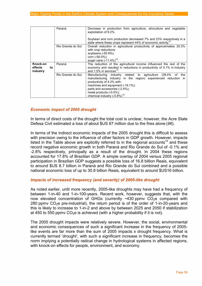
Major Tipping Points in the Earth’s Climate System and Consequences for the Insurance Sector
Page 59
Paraná Decrease in production from agriculture, silviculture and vegetable exploitation of 9.2%. Soybean and corn production decreased 7% and 23% respectively in a state where these crops represent 44% of economic activity14.
Rio Grande do Sul Overall reduction in agricultural productivity of approximately 25.3% with crop reductions: soybeans (-55.9%); corn (-56.0%); sugar cane (-11.4%)14.
Paraná The reduction of the agricultural income influenced the rest of the economy and resulted in reductions in productivity of 0.1% in industry and 1.5% in services14.
Knock-on effects to industry
Rio Grande do Sul Manufacturing industry related to agriculture (39.4% of the manufacturing industry in the region) experienced reduction in productivity of 4.2% with: machines and equipment (-19.1%); parts and accessories (-2.4%); metal products (-0.5%); chemical industry (-5.8%)14.
Economic impact of 2005 drought In terms of direct costs of the drought the total cost is unclear, however, the Acre State Defesa Civil estimated a loss of about $US 87 million due to the fires alone (96). In terms of the indirect economic impacts of the 2005 drought this is difficult to assess with precision owing to the influence of other factors in GDP growth. However, impacts listed in the Table above are explicitly referred to in the regional accounts14 and these record negative economic growth in both Paraná and Rio Grande do Sul of -0.1% and -2.8% respectively, principally as a result of the drought. In 2004 these regions accounted for 17.8% of Brazilian GDP. A simple overlay of 2004 versus 2005 regional participation in Brazilian GDP suggests a possible loss of 16.8 billion Reais, equivalent to around $US 8.7 billion in Paraná and Rio Grande do Sul combined and a possible national economic loss of up to 30.8 billion Reais, equivalent to around $US16 billion. Impacts of increased frequency (and severity) of 2005-like drought As noted earlier, until more recently, 2005-like droughts may have had a frequency of between 1-in-40 and 1-in-100-years. Recent work, however, suggests that, with the now elevated concentration of GHGs (currently ~430 ppmv CO2e compared with 280 ppmv CO2e pre-industrial), the return period is of the order of 1-in-20-years and this is likely to increase to 1-in-2 and above by between 2025 and 2050 if stabilization at 450 to 550 ppmv CO2e is achieved (with a higher probability if it is not). The 2005 drought impacts were relatively severe. However, the social, environmental and economic consequences of such a significant increase in the frequency of 2005-like events are far more than the sum of 2005 impacts x drought frequency. What is currently termed ‘drought’, with such a significant increase in frequency, becomes the norm implying a potentially radical change in hydrological systems in affected regions, with knock-on effects for people, environment, and economy.

Major Tipping Points in the Earth’s Climate System and Consequences for the Insurance Sector
Page 60
3.4.4 Brazil forest die-back: insurance and finance implications Issues at a glance Event description: 70% loss of natural rainforest Region: South America Socio-economic effects: Indirect - acceleration of climate change.
Direct - disruption of carbon markets. Severe local water shortages.
Other aspects: Boreal forest growth may partially offset the carbon loss. Ablation of Andean glaciers exacerbates regional water crisis.
Timing: 2080’s but already apparent by 2020’s (see next comment). Warning: Preceded by sharp increase in drought frequency. Counter-measures: No feasible adaptation to preserve forests.
Solar power could alleviate the decline in hydropower. Type of business
Risks Opportunities
Property Forest restoration, forest products No Casualty Advisory liability No Life/health No No Other Carbon credit delivery No Investment/savings Carbon & biodiversity funds Solar power.
Major impact Key:
Minor impact
Rainforests do not feature materially in financial markets at present, but there are moves to involve private finance significantly, through monetizing the environmental benefits of natural forests (see for example The Princes Rainforest Project, Eliasch Review, UNEPFI, IUCN). In particular, following the Stern Review analysis that avoiding deforestation is one of the most important steps to mitigate climate change, there are proposals to accelerate funding from the private sector to preserve rainforests through, for example, The Prince’s Rainforest Trust(121). This is seen as a stop-gap measure pending political agreement on measures to Reduce Emissions from Deforestation and Forest Degradation (REDD) under the UNFCCC. Tropical forests store a fourth of all terrestrial carbon, i.e. 547 Gt out of 2,052 Gt of CO2. In addition, recent research suggests that tropical forests may capture as much as 4.8 Gt of CO2 per annum (98). Returns might be based on other eco-benefits such as water purification or biodiversity, since carbon sequestration is not the only service provided by forests (99). They provide a wide range of other services, related to provisioning, environmental regulation, and cultural activities. Already, tentative values have been placed on these (see Table 3.4.4 below). Including forest carbon as a major component of a future climate regime could set an important precedent. It can serve as a potential platform for the development of other payments for ecosystem services. Table 3.4.4: Values of ecosystem services in tropical forests (Source: (98)) Ecosystem service type Value of ecosystem services
( $US / ha / year – 2007 values) Provisioning services Food 75 Water 143 Raw materials 431 Genetic resources 483 Medicinal resources 181 Regulating services Air quality 230 Climate 1965 Water flow 1360

Major Tipping Points in the Earth’s Climate System and Consequences for the Insurance Sector
Page 61
Waste disposal & water purity 177 Erosion control 684 Cultural services Recreation and tourism 381 Total 6120
In addition to mitigation, investment in restoring or conserving ecological infrastructure which delivers ecosystem services can significantly enhance agricultural sustainability, especially in developing countries. It can improve freshwater supplies and reduce future insecurity. It can considerably reduce the impacts of natural hazards and extreme weather events. Such investment can also improve skills and create decent jobs in poor communities. Table 3.4.5 gives an indication of the costs and benefits concerned. Table 3.4.5: Costs and benefits of restoration (Source: (98))
Typical cost of restoration
Estimated annual benefits from restoration
(avg. scenario)
Net present value of
benefits over 40 years
Internal rate of return
Benefit/cost ratio
$US / ha $US / ha $US / ha % ratio 3,450 7,000 148,700 50 37.3
Insurers could be involved as investors, or as providers of risk-transfer products relating to the restoration of functionality of the forest due. One estimate of the potential carbon markets in forests is $US 90 billion by 2020 (100). Risk-transfer products Risk-transfer products could be formulated as conventional indemnity products, which pay out after a specified loss, or indexed products, which pay out on the occurrence of specified conditions, in this case abnormal weather. The cover could relate to the cost of restoration of the natural forests, as under EU environmental impairment insurance, or the provision of eco-credits or simply a notional value inherent in the forest. (A fourth type of cover might relate to covering the production of forestry-based goods such as textiles, food, timber, medicines, etc.). Insurance of forests is a very minor activity compared to other insurance products, due to the difficulty of monitoring damage and controlling losses. These problems are severe for managed forests, and very severe for natural forests. Even the introduction of new technologies such as remote observation will not materially change the position as far as rainforests are concerned, due to the absence of damage control facilities. Finally, insurers might be involved as providers of cover to decision-makers or advisers who are involved with forestry assets. This risk is unlikely to be significant since cover is normally restricted in quantum, and reliant on evidence of good practice by the insured party. Investment Potentially, long-term insurers (i.e. life/pensions/savings) could view natural forestry assets as appropriate vehicles for their clients and beneficiaries, in the same way as they do with managed forests. Currently, this is not a significant component of their
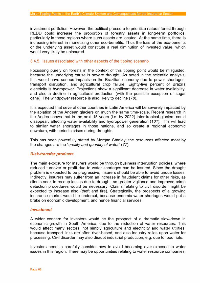
Major Tipping Points in the Earth’s Climate System and Consequences for the Insurance Sector
Page 62
investment portfolios. However, the political pressure to prioritize natural forest through REDD could increase the proportion of forestry assets in long-term portfolios, particularly in those regions where such assets are located. At the same time, there is increasing interest in monetizing other eco-benefits. Thus the loss of the eco-benefits or the underlying asset would constitute a real diminution of invested value, which would very likely be uninsured. 3.4.5 Issues associated with other aspects of the tipping scenario Focussing purely on forests in the context of this tipping point would be misguided, because the underlying cause is severe drought. As noted in the scientific analysis, this would have serious impacts on the Brazilian economy due to power shortages, transport disruption, and agricultural crop failure. Eighty-five percent of Brazil’s electricity is hydropower. Projections show a significant decrease in water availability, and also a decline in agricultural production (with the possible exception of sugar cane). The windpower resource is also likely to decline (78). It is expected that several other countries in Latin America will be severely impacted by the ablation of the Andean glaciers on much the same time-scale. Recent research in the Andes shows that in the next 15 years (i.e. by 2022) inter-tropical glaciers could disappear, affecting water availability and hydropower generation (101). This will lead to similar water shortages in those nations, and so create a regional economic downturn, with periodic crises during droughts. This has been powerfully stated by Morgan Stanley: the resources affected most by the changes are the “quality and quantity of water” (77). Risk-transfer products The main exposure for insurers would be through business interruption policies, where reduced turnover or profit due to water shortages can be insured. Since the drought problem is expected to be progressive, insurers should be able to avoid undue losses. Indirectly, insurers may suffer from an increase in fraudulent claims for other risks, as clients seek to recoup losses due to drought, so greater vigilance and improved crime detection procedures would be necessary. Claims relating to civil disorder might be expected to increase also (theft and fire). Strategically, the prospects of a growing insurance market would be undercut, because endemic water shortages would put a brake on economic development, and hence financial services. Investment A wider concern for investors would be the prospect of a dramatic slow-down in economic growth in South America, due to the reduction of water resources. This would affect many sectors, not simply agriculture and electricity and water utilities, because transport links are often river-based, and also industry relies upon water for processing. Civil disorder may also disrupt industrial production, e.g. due to food riots. Investors need to carefully consider how to avoid becoming over-exposed to water issues in this region. There may be opportunities relating to water resource companies,

Major Tipping Points in the Earth’s Climate System and Consequences for the Insurance Sector
Page 63
e.g. water purification and recycling, and in other sectors, e.g. security or construction, but the downside of water shortage needs to be carefully analysed. On the positive side, the region is relatively well-placed with respect to solar power resources, which have not been targeted there due to other resources which may become problematic (hydro, biofuel, and fossil fuels). This could be a significant growth area in future. 3.5 Increased aridity in Southwest North America 3.5.1 Overview As described in Section 2, aridity in south-western North America is predicted to intensify and persist in future and a transition is probably already underway and will become well established in the coming years to decades, akin to permanent drought conditions (4). Levels of aridity seen in the 1950s multiyear drought or the 1930s Dust Bowl are robustly predicted to become the new climatology by mid-century, resulting in perpetual drought (102). This is a robust result in climate model projections because it has its source in well-represented changes in the atmospheric hydrological cycle related to both rising humidity in a warmer atmosphere and poleward shifts of atmospheric circulation features. Applying 19 climate models to the history and future of annual mean precipitation minus evaporation (P - E) Seager et al. (4) used a multiple model approach to examine trends and, therein, likelihood of increasing aridity in the American Southwest (defined as land cover within 125°W to 95°W and 25°N to 40°N). This shift is illustrated in Figure 3.5.1 which provides average deviation in P - E over 20-year periods relative to model climatologies from 1950–2000 for each of the models15 reported by Seager et al.. For comparison, conditions similar to those experienced during the ‘dust bowl drought’ of the 1930s and the 1950s ‘Southwest drought’ (around - 0.1 mm of daily precipitation16) are overlaid onto the figure. Similarly, Figure 3.5.2 (based on (4)) provides the change in annual mean P - E over the American Southwest for four coupled models providing an idea of plausible evolutions of Southwest climate towards a more arid state. Both figures suggest either an imminent or already triggered switch towards extended periods of sustained drought.
15 The number of ensemble members for each projection is listed with the model name on the left. Black dots represent ensemble members (where available) and red dots represent the ensemble mean for each model. 16 Annual mean reduction in P for this region, calculated from rain gauge data within the Global Historical Climatology Network, was 0.09 mm/day between 1932 and 1939 (the Dust Bowl drought) and 0.13 mm/day between 1948 and 1957 (the 1950s Southwest drought) – Seager et al. (2007).
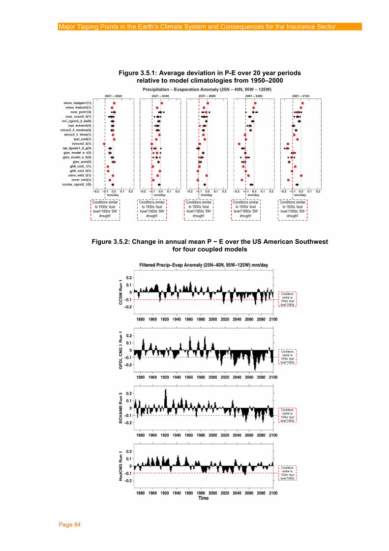
Major Tipping Points in the Earth’s Climate System and Consequences for the Insurance Sector
Page 64
Figure 3.5.1: Average deviation in P-E over 20 year periods relative to model climatologies from 1950–2000
Figure 3.5.2: Change in annual mean P − E over the US American Southwest for four coupled models
Conditions similar to 1930s ‘dust
bowl’/1950s ‘SW drought’
Conditions similar to 1930s ‘dust
bowl’/1950s ‘SW drought’
Conditions similar to 1930s ‘dust
bowl’/1950s ‘SW
drought’
Conditions similar to 1930s ‘dust
bowl’/1950s ‘SW
drought’
Conditions similar to 1930s ‘dust
bowl’/1950s ‘SW drought’
Conditions similar to
1930s ‘dust bowl’/1950s
Conditions similar to
1930s ‘dust bowl’/1950s
Conditions similar to
1930s ‘dust bowl’/1950s
Conditions similar to
1930s ‘dust bowl’/1950s

Major Tipping Points in the Earth’s Climate System and Consequences for the Insurance Sector
Page 65
3.5.2 Impacts of a shift to a more arid state by reference to historical parallels In terms of predicting and assessing impacts of changes in conditions, it is usual to examine and compare with historical events of a similar nature. Here, comparison has already been made with conditions seen in the 1950s multiyear drought or the 1930s Dust Bowl. However, it is important to note that, while conditions are similar, the future intensified aridity in the Southwest predicted by Seager et al. (4) is caused by different processes and expected drying is “unlike any climate state we have seen in the instrumental record”. The six severe multiyear droughts that have struck western North America in the instrumental record have all been attributed to variations in sea surface temperatures (SSTs) in the tropics (particularly persistent La Niña-like SSTs in the tropical Pacific Ocean). The multidecadal megadroughts that afflicted the American Southwest during Medieval times have also been attributed to changes in tropical SSTs. The combined effect of the processes driving future aridity (4) and existing primary causes of drought in SWNA (SSTs) is that the most severe future droughts will still occur during persistent La Niña events, but they will be worse than any since the Medieval period, because the La Niña conditions will be perturbing a base state that is drier than any state experienced recently (4). This means that the anticipated shift to sustained and much drier conditions is one for which there is no obvious recent parallel to draw upon. In addition, while the closest parallel would seem to be conditions in the 1950s or 1930s, social and cultural factors strongly mediated the expression of impacts and their resulting severity. Here, for example, the 1930s ‘Dust Bowl’ occurred during the Great Depression and one of the greatest population movements in United States history occurred. The drought-prone wheat that the farmers had planted shrivelled and died, ploughs had torn out the native, drought resistant prairie grass in the preceding years of ample rain and food demand and winds tore at the bare soil removing valuable topsoil in `black blizzards' and dumped it as far away as Washington D.C. and even Norway (102). Accordingly, whilst there may be parallels in terms of climatological conditions, the factors mediating the expression of impact are not only significant but are likely to be significantly different from today’s situation (and in future) making estimation of future impacts by direct comparison with historical drought impacts problematic. 3.5.3 Impacts of a shift to a more arid state by reference to existing trends and
projections (SW United States) In terms of a comparison with existing climatological trends, at first sight, a reduction in daily precipitation of around -0.1 mm or 15% would seem relatively small. However, it is important to note that it is not the magnitude of the reduction in precipitation in a single year that is of significance but the persistence of such conditions over a period of years. During the 1930s Dust Bowl, for example, precipitation over the Great Plains was reduced by about 15%, but when this happens year after year, the ground moisture is progressively reduced as evaporation proceeds, resulting in severe drought over an extended period (measured in years or decades).

Major Tipping Points in the Earth’s Climate System and Consequences for the Insurance Sector
Page 66
As such, unlike the future droughts in India (discussed in Section 3.3), the case of SWNA droughts relates to sustained long periods (measured in years to decades) of relatively small shortfalls in precipitation as opposed to the frequency of more significant deviations in the timing and magnitude of precipitation (such as the periodic failure of monsoon rains). Predictions of future increasing aridity in SWNA are not peculiar to the work of Seager et al. (4) at the University of Columbia, and work being undertaken as a result of the June 2005 California State Executive Order17 also works on the basis of predictions of increased drying, albeit not over the same (short) time-scales or severity (in terms of both P - E and duration). For example, based on projections using IPCC SRES A2 and B1 emissions scenarios, the Climate Action Team (CAT) Draft Biennial Report (103) identifies the following: • a high degree of variability from year to year of annual precipitation will prevail over
this century including a continued vulnerability to drought; • in the northern part of California, the tendency for drying fades and even reverses
but in Southern California the amount of drying becomes greater, with decreases in precipitation in some simulations exceeding 15%;
• even if precipitation levels were to remain unchanged over the 21st century, the
higher temperatures would increase evaporative water loss and thus produce overall drier conditions.
Whilst such California State investigations do not seem to work on the basis of increasing aridity with the imminence and severity of the projections of Seager et al. (4), they do provide some insight and context to issues and problems associated with future aridity in California, albeit only with reference to current trends and less extreme projections. Here, key impacts of most concern are likely to divide broadly into impacts on • water resources, • agriculture, and • wildfires. Headline trends and impacts that contextualize the impact of increased aridity in SWNA are provided below.
17 This initiated a process of biennial updates on the state of climate change science, impacts and adaptation in California.

Major Tipping Points in the Earth’s Climate System and Consequences for the Insurance Sector
Page 67
Water resources Water resource management under a changing climate could emerge as California’s greatest future challenge. Satisfying the water needs for the state’s industrial, urban, agricultural, energy, and environmental uses will be harder owing to a combination of a decreasing reliability of surface water storage and anticipated population growth (104). In terms of the latter, the population of California is expected to grow by 14 million overall with most of this growth occurring in Southern California, resulting in a geographic disconnect between demand and supply. Dry Southern California imports water from the wetter north, yet the population in Southern California is growing faster than elsewhere in the state (PPIC, 2006). In addition, an aging and increasingly immigrant population in the southern part of the state is contributing to growing social vulnerability there compared to other regions of the state (104). In terms of surface water resources, an important trend identified in Government of California work (104) is the decline of total snow accumulation (and water content in the snow) on April 1st, the date which determines how much water will be available to satisfy water demands in the spring and summer (104). Consistent with the decreasing spring snow levels, California, as well as most of the western United States, is experiencing a related decrease in the fraction of total run-off occurring in the spring. Spring run-off provides a significant portion of the water supply for dry summers and autumns in California and over the past 100 years the fraction of the annual run-off that occurs during April–July has decreased by 23% for the Sacramento basin and 19% for the San Joaquin basin (104). In the southern part of the state, water supplies from the Colorado River may decrease in the future and a recent comprehensive modelling study projected an 8–11 % decrease in run-off by 2100 for the Colorado River Basin depending on the emissions scenario (104). In terms of groundwater resources, currently about half of California’s water supply for human consumption or use comes from groundwater and future management of groundwater will be critical in the next century against the background of surface water supplies being insufficient to accommodate the water needs of the state’s growing population and economy (104). As natural precipitation already varies greatly throughout California, a large infrastructure geared towards moving water from areas of abundance to places of relative scarcity has been developed. However, a recent estimate of the cost impacts of a dry warming scenario suggests an increase in state-wide water scarcity and total operation costs by at least $US 500 million per year by 2085. The actual total costs may be two to three times higher because the original authors assume perfect water markets and do not consider other potential costs associated with climate change and, as such, the estimates do not include operational costs of measures (for example for flood protection) or recovery costs (for example, in the event of floods) (104). In terms of market functioning, in future decades, greater interaction in regional water markets will be required. Reduction in water availability will require that all states, particularly within the Colorado River watershed, will need to collaborate and share the diminishing water resources fairly. Much of the West, like California, is considering

Major Tipping Points in the Earth’s Climate System and Consequences for the Insurance Sector
Page 68
some use of groundwater sources to supplement shrinking water supplies but groundwater access and rights among multiple regional players is subject to debate as is reportedly occurring in the area surrounding Las Vegas, which is experiencing tremendous population and development growth (104). There is also an international dimension to water trading (and conflict) as Mexico is also expected to suffer increasing and sustained drought with potentially severe consequences (see Section 3.5.3). Agriculture Agriculture in California represents an economically and culturally important activity that contributes substantially to national and international production of many commodities. State-wide agricultural income from sales in 2003 was $US 27.8 billion, or 13% of the U.S. total (2004). As the nation’s leading producer of 74 different crops, California supplies more than half of all domestic fruit and vegetables (105). California is also responsible for more than 90% of the nation’s production of almonds, apricots, raisin grapes, olives, pistachios, and walnuts (104). Despite advances in technology and the widespread prevalence of irrigation in the state, agricultural production remains highly dependent on weather, which can affect both the quantity and quality of harvested crops (105). Crop response to climate change is complicated by a number of factors and changes including in precipitation, temperature averages, maxima and minima, pest and weed ranges, the length of the growing season, and other factors (104). A study examining changes in these factors and effects on productivity of seven annual field crops from 1950–2099 suggested that climate change will decrease annual crop yields in the long term, particularly for cotton, unless future climate change is minimized and/or adaptation of management practices and improved cultivars become widespread (104). Wildfire Climate change impacts on wildfire risk and severity are a function of elevated temperatures, potentially increasing the vegetative fuel load (in wetter years) and drying out vegetation (in drier years that are predicted). In addition to destruction of large areas, wildfire impacts upon a number of economic and environmental factors including air pollution, visibility, and human health (from smoke and aerosols), ecosystem dynamics, wildlife habitat, timber production, hydrological systems, flooding, and soil erosion risks (from loss of forest cover) (104). In terms of projections for SRES scenarios estimates, the long-term increase in fire occurrence associated is substantial, with state-wide increases ranging from 58–128% by 2085 and estimated burned area increasing 57–169% under the A2 pathway (104). Projections of changes over time and a scenario are provided in Figure 3.5.3.
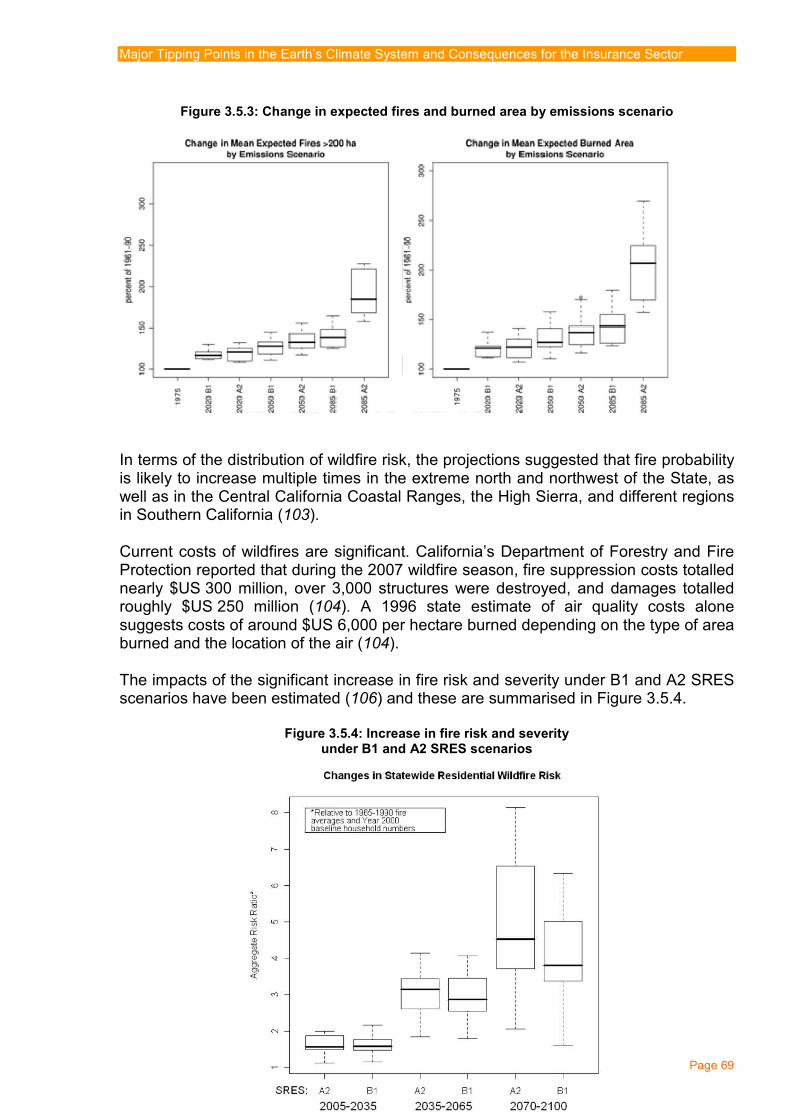
Major Tipping Points in the Earth’s Climate System and Consequences for the Insurance Sector
Page 69
Figure 3.5.3: Change in expected fires and burned area by emissions scenario
In terms of the distribution of wildfire risk, the projections suggested that fire probability is likely to increase multiple times in the extreme north and northwest of the State, as well as in the Central California Coastal Ranges, the High Sierra, and different regions in Southern California (103). Current costs of wildfires are significant. California’s Department of Forestry and Fire Protection reported that during the 2007 wildfire season, fire suppression costs totalled nearly $US 300 million, over 3,000 structures were destroyed, and damages totalled roughly $US 250 million (104). A 1996 state estimate of air quality costs alone suggests costs of around $US 6,000 per hectare burned depending on the type of area burned and the location of the air (104). The impacts of the significant increase in fire risk and severity under B1 and A2 SRES scenarios have been estimated (106) and these are summarised in Figure 3.5.4.
Figure 3.5.4: Increase in fire risk and severity under B1 and A2 SRES scenarios

Major Tipping Points in the Earth’s Climate System and Consequences for the Insurance Sector
Page 70
Table 3.5.1 presents the economic losses in relation to the revenues that land owners would realize in the absence of climate change (103). Estimates do not include impacts from expanded ranges of pests or disease. Forest fires damages reflect only potential impacts on housing units. Table 3.5.1: Loss in undiscounted cumulative net revenue from timber production in California and annual damages from forest fires on housing units (loss in undiscounted cumulative revenue in $US billion; fire damages in $US billion/year) Climate Scenario Impact 2050 2085
Timber revenue -0.4 to 3.4 4.2 to 8.0 A2 Forest fires 0.2 to 2.3 0.7 to 14 Timber revenue -2.2 to -1.3 - B1 Forest fires 0.2 to 2.5 0.5 to 11
Negative numbers represent gains. Estimates for undiscounted cumulative timber revenue from Hannah et al., (2008) (107). Losses calculated from 2000 through to 2050 or 2080. Estimates for annual damages from forest fires from Bryant and Westerling (2008) for 2050 and 2085 (106).
3.5.4 Regional impacts outside the SW United States Besides South-western North America other land regions to be hit hard by subtropical drying include southern Europe, North Africa and the Middle East as well as parts of South America (4) (see inset). Even in terms of the impacts in SWNA, aridity is not restricted to the SW of the United States and is predicted to have significant impacts in Mexico, with possible implications not only for populations in Mexico itself, but also wider implications for the wider geo-political region. If the model projections are correct, México faces a future of declining water resources that will have serious consequences for public water supply, agriculture, and economic development and this will (and has) affected the region as a whole, including the United States (108). México has already experienced a severe, if not unprecedented, drought that began in the mid 1990s and at least continued through the first few years of the current century. This accompanied far-reaching structural changes in the Mexican economy and agriculture arising from the North American Free Trade Agreement (NAFTA) and amidst ongoing privatization of formerly communal land and water rights. NAFTA stimulated industrial growth in the semi-arid north and encouraged commercial farmers to move toward alfalfa and export crops, especially fruit and vegetables that are all

Major Tipping Points in the Earth’s Climate System and Consequences for the Insurance Sector
Page 71
water intensive, while the 1992 reform of Mexico’s basic hydraulic law opened the door to market-based water pricing (108). In the face of protracted drought and rising water demand by export-oriented farmers, border industrial plants (‘maquiladoras’) and growing cities in northern Mexico, numerous ‘water wars’ were initiated between different communities and user groups, including an international conflict over Chihuahua’s inability to supply downstream Texan farmers with treaty-allocated Rio Bravo/Grande water (108). The recent drought has primarily affected northern México but global warming-associated climate change is projected to cause drying of the whole of México (108). 3.5.5 Key implications for insurers of increased aridity in Southwest North America Issues at a glance Event description: Drought Region: SW North America Socio-economic effects: Harvest failure, industrial interruption, wildfire Timing: Before 2050 Warning: Yes - progressively worse events. Countermeasures: Solar power, desalination ( for energy and non-agriculture). Type of business Risks Opportunities
Property Wildfire No Casualty Advisory liability No Life/health Disease No Other Crop failure, interruption More demand All insurance Slump in demand, fraud, crime No Investment/savings Economic blight in region Countermeasure sectors
Major impact Key:
Minor impact
The most significant impact of the tipping point from an insurer’s perspective is likely to be water shortage, leading to wildfire and economic disruption in water, agriculture, energy, and tourism. The combined effects of natural climate variability and human-induced climate change could turn out to be a devastating ‘one-two punch’ for the region. As of 2009, much of the Southwest remains in a drought that began around 1999. This event is the most severe western drought of the last 110 years, and is being exacerbated by record warming (109). Human and industrial needs can be maintained even in a very severe drought by closing down the supply to agriculture. The energy and tourism sector cannot be protected in the same way because they depend on water availability in fixed locations. A recent study suggests that radically improved water efficiency in the agricultural sector could reduce water use in that sector by 17%, and thereby preserve the agricultural sector (110). However, in California irrigation water is predominantly delivered through canals and provided on a pre-ordered or rotational basis (117) rather than on-demand, which is a necessary precondition for many on-farm water efficiency improvements. In addition, the report would require the introduction of water pricing

Major Tipping Points in the Earth’s Climate System and Consequences for the Insurance Sector
Page 72
tariffs, and it is based on projections of precipitation which are not as severe as the ‘tipping point’ scenario proposed in the present analysis (less than 10% reduction by mid-century, compared to 15% here (111). Critical repercussions from this water shortage will probably be massive job losses for unskilled workers, many of them immigrants. Essentials such as food, energy and water will become more expensive, exacerbating their plight. This is likely to lead to a large increase in crime, both against third parties (vandalism and theft), as well as fraud, e.g. dishonest insurance claims. Given the importance of the agriculture industry in SWNA, a collapse in output will result in knock-on effects in transportation, storage, and real estate values. Public sector finances will be impaired, with possible defaults. At the same time, it is important to realize that climate change will cause other disruptions to the SWNA region. In particular, flooding will become more serious (111), due to the changing seasonality of rainfall and the faster run-off on sun-baked surfaces, and also in the coastal zone, due to subsidence coupled with sea level rise. The entire California Delta region is now below sea level, protected by more than a thousand miles of levees and dams. This will complicate the situation and divert resources (e.g. for flood defence). Projected changes in the timing and amount of river flow, particularly in winter and spring, is estimated to more than double the risk of Delta flooding events by mid-century, and result in an eight-fold increase before the end of the century. Taking into account the additional risk of a major seismic event and increases in sea level due to climate change over this century, the California Bay–Delta Authority has concluded that the Delta and Suisun Marsh are not sustainable under current practices; efforts are underway to identify and implement adaptation strategies aimed at reducing these risks. Another landscape where flood risk could become more serious is alluvial fans. These are gently sloping fan-shaped landforms created over long periods of time by the deposition of eroded sediment from an upland source. Such areas comprise over 40 percent of the landscape in Southern California. Significant areas have already been urbanized (118). Debris flows during floods there are very hazardous; those that followed wildfires in southern California in 2003 killed 16 people and caused tens of millions of dollars of property damage. Rainfall that is normally absorbed into hill slopes can run off almost instantly after vegetation has been removed by wildfire. Highly erodible soils in a burn scar allow flood waters to entrain large amounts of ash, mud, boulders, and unburned vegetation. (119). To date, climate change has not been systematically incorporated into risk assessment here (120). A study has been carried out to assess the risks, given that the Fourth IPCC Assessment Report (AR4) understated the likely sea level rise. It is estimated that a 1.4 metre sea level rise will put 480,000 people at risk of a 100-year flood event, without further population growth. The cost of replacing property at risk of coastal flooding under this post-AR4 sea level rise scenario is estimated to be nearly $US 100 billion in year 2000 dollars (112). Protecting key areas from flooding by building sea defences will cost at least $US 14 billion (in year 2000 dollars), with maintenance costs of another $US 1.4 billion per year. Uncontrolled development could increase the exposure and costs substantially.

Major Tipping Points in the Earth’s Climate System and Consequences for the Insurance Sector
Page 73
State-wide flood risk exceeds erosion risk, but in some counties and localities, coastal erosion poses a greater risk. A 1.4 metre sea level rise will accelerate erosion, resulting in a loss of 41 square miles (over 10,500 hectares) of California’s coast by 2100. The infrastructure at risk includes nearly 140 schools, 34 police and fire stations, 55 healthcare facilities, over 330 hazardous waste facilities or sites, 3,500 miles of roads and highways and 280 miles of railways, 30 coastal power plants with a combined capacity of more than 10,000 megawatts, 28 wastewater treatment plants with a combined capacity of 530 million gallons per day, and the San Francisco and Oakland airports. Insurance in California California is one of the world’s largest insurance markets. If it were an independent country, it would rank 7th for total insurance expenditure in 2008 (excluding the USA itself), with the non-life market being slightly lower at 8th. Growth in real terms has been almost absent since 1999, allowing some national markets (such as China) to overtake California, but it is still an enormously important arena. Table 3.5.2: The Californian insurance market (Source: California Statistical Abstract, 2008; Swiss Re Sigma series) Premiums
($US mill., 2008) World Ranking (2008)
Real growth 1999/2008
Premiums as % GDP (2008)
Premiums per capita ($US, 2008)
Total 121,319 7th 2% 6.9 3,192
Life 67,993 7th 3.9 1,780 Non-life 53, 946 8th 3.0 1,412
In 2004 there were 1,279 insurers in the State, with $US 23 billion invested in municipal bonds (113). When considering statistics on insured losses, it is important to bear in mind that, as with other US states, there is a significant proportion of uninsured auto drivers, that only a minority of home-owners have earthquake insurance, and that nearly two-thirds (64%) of all homes in America are underinsured by an average of 27%. Figure 3.5.5 shows that wildfire is a significant cost to insurers in California. The fire season has extended by over two months, and this hazard is a factor in recent rate increases approved by the regulators. It could even become a material fact in insurers’ credit rating (114). Wildfire claims are not just an issue for property insurers. Insured and uninsured losses can be recovered under liability policies, e.g. where energy companies have negligently permitted power lines to cause a fire. (However, many fires are the result of criminal activity by private individuals). In addition, legislators are considering a surcharge of nearly 3% on insurance premiums to cover the cost of fire-fighting. Ironically this could have a negative effect on insurance take-up, since consumers are price-sensitive.
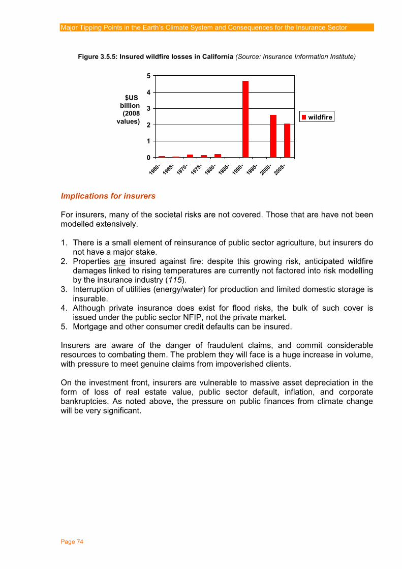
Major Tipping Points in the Earth’s Climate System and Consequences for the Insurance Sector
Page 74
Figure 3.5.5: Insured wildfire losses in California (Source: Insurance Information Institute) Implications for insurers For insurers, many of the societal risks are not covered. Those that are have not been modelled extensively. 1. There is a small element of reinsurance of public sector agriculture, but insurers do
not have a major stake. 2. Properties are insured against fire: despite this growing risk, anticipated wildfire
damages linked to rising temperatures are currently not factored into risk modelling by the insurance industry (115).
3. Interruption of utilities (energy/water) for production and limited domestic storage is insurable.
4. Although private insurance does exist for flood risks, the bulk of such cover is issued under the public sector NFIP, not the private market.
5. Mortgage and other consumer credit defaults can be insured. Insurers are aware of the danger of fraudulent claims, and commit considerable resources to combating them. The problem they will face is a huge increase in volume, with pressure to meet genuine claims from impoverished clients. On the investment front, insurers are vulnerable to massive asset depreciation in the form of loss of real estate value, public sector default, inflation, and corporate bankruptcies. As noted above, the pressure on public finances from climate change will be very significant.
0
1
2
3
4
5
1960-
1965-
1970-
1975-
1980-
1985-
1990-
1995-
2000-
2005-
wildfire
$US billion (2008
values)

Major Tipping Points in the Earth’s Climate System and Consequences for the Insurance Sector
Page 75
4. Summary of impacts and concluding thoughts 4.1 Summary of key impacts and contexts 4.1.1 Overview Based on the discussion in Sections 2 and 3, tipping scenarios most likely to have impacts within (or beginning) by the middle of the 21st century include: • global sea level rise (SLR) of up to 2 m by the end of the century (combined GIS,
WAIS) combined with localized sea level rise anomaly (on top of global SLR) for the eastern seaboard of North America (THC);
• shifts in hydrological systems in Asia as a result of
o hydrological disturbance of monsoon hydrological regimes particularly Indian Summer Monsoon (from Brown Cloud forcing and ENSO); and
o disturbance of fluvial systems fed from the Hindu-Kush-Himalaya-Tibetan glaciers (HKHT);
• committed die-back of the Amazon Rainforest and a significant increase in the
frequency of the North Atlantic anomaly responsible for the 2005 drought in western and southern parts of the Amazon basin; and
• a significant shift to a very arid climatology in SWNA. Context The subsections below briefly summarize the costs and impacts of these tipping scenarios. When considering these impacts it is important to bear in mind the current state of affairs with regard to emissions and projected global temperature rise. This can be summarised as follows: • to provide a 93% mid-value probability of not exceeding, say, 2 °C, the
concentration of greenhouse gases would need to be stabilized at, or below, 350 parts per million by volume of CO2e;
• current greenhouse gas concentration is estimated to be 430 ppmv CO2e and, as
such, global atmospheric GHG concentrations already exceed those necessary to avoid, say, a 2 °C global temperature rise with some degree of certainty/probability;
• stabilization at 450 ppmv CO2e is estimated to only provide between a 26%–78%
chance of not exceeding 2 °C or, put another way, between a 22% and 74% chance of exceeding 2 °C;
• stabilization at 550 ppmv CO2e is estimated to provide between a 63% and 99%
chance of exceeding 2 °C; and

Major Tipping Points in the Earth’s Climate System and Consequences for the Insurance Sector
Page 76
• stabilization at either of these concentrations still, however, requires emissions to peak around 2015 with annual reductions in global emissions of several percent per year needing to be sustained year on year throughout this century.
4.1.2 Summary of impacts - combined sea level rise A ‘tipping’ scenario of around 0.5 m of global SLR by 2050 is a reasonable starting assumption for the analysis. Added to this, a regional dynamic sea level change of 0.15 m added to the global SLR of 0.5 m (to give a total of 0.65 m) by 2050 provides a reasonable but higher end estimate for a ‘tipping’ scenario for the NE coast of the USA. Exposed assets in port megacities under a global 0.5 m tipping scenario A global sea level rise of 0.5 m by 2050 is estimated to increase the value of assets exposed in all 136 port megacities worldwide by a total of $US 25,158 billion to $US 28,213 billion in 2050. This increase is as a result of changes in socio-economic factors such as urbanization and also increased exposure of this (greater) population to 1-in-100-year surge events through sea level rise. Exposed assets on NE coast of the US with an additional 0.15 m additional SLR In terms of the impact of the additional 0.15 m of SLR affecting the NE Coast of the USA the following port megacities may experience a total sea level rise of 0.65 m by 2050: Baltimore, Boston, New York, Philadelphia, and Providence. Here, 0.65 m of SLR is estimated to increase asset exposure from a current estimated $US 1,359 billion to $US 7,425 billion. The additional asset exposure from the regional anomaly alone (i.e. 0.65 versus 0.5 mm) is approximately $US 298 billion (across the above-mentioned cities alone). Insurance aspects The critical issue is the impact that a hurricane in the New York region would have. Potentially the cost could be 1 trillion dollars at present, rising to over 5 trillion dollars by mid-century. Although much of this would be uninsured, insurers are heavily exposed though hurricane insurance, flood insurance of commercial property, and as investors in real estate and public sector securities. 4.1.3 Summary of impacts - Indian Summer Monsoon The impacts on hydrological systems in India under a ‘tipping’ scenario are comprised of • atmospheric brown cloud forcing – which is predicted to interfere with the Indian
Summer Monsoon (ISM) to approximately double drought frequency (2) from an average of around 2 per decade (for the period 1800–2000) to 4 per decade in the first half of this century; and

Major Tipping Points in the Earth’s Climate System and Consequences for the Insurance Sector
Page 77
• changes in ENSO amplitude – ENSO is known to cause variation in the Indian Summer Monsoon. In response to a stabilized 3–6 °C warmer climate, the most realistic models simulate increased El Niño amplitude (with no change in frequency).
In addition to the effects on monsoon rainfall, melting of the Himalayan glaciers is expected to reduce river flows. Drought costs Extrapolating from the 2002 drought using a simple calculation would suggest that the future costs (in today’s prices) might be expected to double from around $US 21 billion to $US 42 billion per decade in the first half of the century. This is likely to be an underestimate owing to a range of other factors that will influence cost and consequence in the same period. Here, there are a number of factors that will act to reduce the extent to which surpluses and irrigation are likely to moderate the impacts in future. The most significant of these are likely to be the combined effects of • decreasing probability of consecutive ‘non-drought’ years from which to accumulate
surpluses; • the pressures of increasing population on food and food surpluses; and • impacts of climate change on irrigation. In terms of the former, the probability of two consecutive ‘non-drought’ years to develop a surplus is halved from 64% to 36% and for three consecutive years the probability is reduced by more than half from 51% to 22%. In both cases the likelihood of consecutive non-drought years is, in future, less than the (40%) probability in any year of a drought. Considering all of the impacts and socio-economic changes under a tipping scenario, namely • a doubling of drought frequency, • up to a 60% reduction in dry season river flows, • population growth pressure to increase production by >40% by 2020 (and continue
after), and • population increase to 1.5 billion by 2050, the effect of all of the variables is to increase the likelihood, severity and exposure of populations and the economy to potentially devastating conditions. It can be concluded that the elements together provide something of a ‘perfect storm’ within the first half of this century with implications for water resources, health, and food security, as well as major economic implications not only for India but for economies regionally and worldwide.

Major Tipping Points in the Earth’s Climate System and Consequences for the Insurance Sector
Page 78
Insurance aspects The potential scale of drought losses could abort the initiatives to extend insurance more widely into the rural sector. The wider repercussions of drought through an economic slow-down and deterioration in public finances would impact insurers strongly, through the liquidation of private savings and the impairment of investments in public sector securities. 4.1.4 Summary of impacts - Amazon The Amazon rainforest is sensitive to changes in both ENSO and the THC and suffers drying during El Niño events and when the North Atlantic is unusually warm. This is expected to result in an increase in both the frequency and severity of drought conditions such as those which occurred in 2005 in western and southern parts of the Amazon basin. In addition to increases in drought frequency and severity, several model studies have now shown the potential for significant die-back of the Amazon rainforest by late this century and into the next. Amazon die-back A number of studies (37, 89, 90) have now shown positive feedbacks that reduce the natural uptake of carbon by alterations in ecosystem functioning and, in relation to the Amazon rainforest, forest die-back under climate change. The most recent work (by Jones et al., 2009) suggests that ecosystems can be committed to long-term change long before any response is observable. Apart from the significant social, environmental, and economic impacts, the loss of very substantial areas of forest will result in the release of significant quantities of CO2. The data suggest that stabilization at, say, 2 °C results in GHG emissions from Amazon die-back equivalent to ~20% of the global historical emissions from global land use change since 1850 and annual emissions (post 2050) equivalent to ~20% of the current (2006–07) global net annual emissions from land use change. As such, committed Amazon die-back has the potential to interfere very significantly with emissions stabilization trajectories in the latter half of the century and moving forward into the future. At present, these emissions are not considered as part of assessments to establish global pathways to climate (or climate impact) stabilization. In terms of the cost of Amazon die-back, any estimate is likely to fall far short of the global economic costs and changes in terms of Total Economic Value (TEV). An indication of the scale of the costs has been derived by application of the shadow price of carbon18. This suggests that • the significant increase in committed die-back that occurs between 1 and 2 °C
results in incremental NPV costs of carbon approaching $US 3,000 billion;
18 Following UK guidance on the appraisal of measures to limit GHG emissions using the shadow price of carbon and applying discounting to provide a net present value (NPV) of carbon emissions according to the UK Treasury Green Book guidelines.

Major Tipping Points in the Earth’s Climate System and Consequences for the Insurance Sector
Page 79
• policies aimed at stabilization at 2 °C result in NPV costs of the order of $US 3,000
billion from carbon lost through committed forest die-back (some 1.6 million km2 of Amazon rain forest); and
• beyond ~2 °C the costs of committed die-back rise very rapidly and more than
double to around $US 7,800 billion and $US 9,400 billion NPV for 3 °C and 4 °C respectively (with forest area losses of around 3.9 million km2 and 4.3 million km2).
Amazon drought In 2005, large sections of the western Amazon basin experienced severe drought resulting in significant impacts in a number of regions. Recent studies (3) investigating the anomaly suggest that droughts similar to that of 2005 will increase in frequency. The drought in 2005 was an approximately 1-in-20-yr event and this is likely to increase to 1 in 2 and above between 2025 and 2050 if stabilization at 450 to 550 ppmv CO2e is achieved (with a higher probability if it is not). The drought of 2005 resulted in a range of impacts including increases in wildfire (with knock-on effects including human health and closure of airports, schools, and businesses), interference with navigation (and therefore trade), reductions in agricultural productivity (with knock-on effects to industries servicing agri-businesses and food shortages) and impacts on hydroelectric power generation (which supplies 85% of Brazil’s electricity). These impacts reduced contribution to Brazilian GDP in affected regions including Mato Grosso do Sul, Santa Catarina, Paraná, and Rio Grande do Sul. In terms of direct costs of the drought the total cost is unclear, however, the Acre State Defesa Civil estimated a loss of about $US 87 million due to the fires alone (96). In terms of the indirect economic impacts of the 2005 drought this is difficult to assess with precision owing to the influence of other factors in GDP growth. However, based on a simple overlay of 2004 versus 2005 regional participation in Brazilian GDP suggests a possible loss of 16.8 billion Reais, equivalent to around $US 8.7 billion in Paraná and Rio Grande do Sul combined and a possible national economic loss of up to 30.8 billion Reais, equivalent to around $US 16 billion. Whilst the 2005 drought impacts were relatively severe, the social, environmental and economic consequences of such a significant increase in the frequency of 2005-like events are far more than the sum of 2005 impacts x drought frequency. What is currently termed ‘drought’, with such a significant increase in frequency, becomes the norm, implying a potentially radical change in hydrological systems in affected regions, with knock-on effects for people, environment, and economy.
Major Tipping Points in the Earth’s Climate System and Consequences for the Insurance Sector
Page 80
Insurance aspects Insurers would be directly affected by the economic effects of drought in the region i.e. an economic slow-down, and deterioration in public finances. The impacts on natural forests would be less material, since markets in natural carbon and biodiversity are unlikely to be significant for some time, and the drought risk will become evident during that period. In a broader sense, drought could incentivize investment into other forms of energy, e.g. solar power. 4.1.5 Summary of impacts - Shift in aridity in Southwest North America (SWNA) Aridity in South-western North America is predicted to intensify and persist in future and a transition is probably already underway and will become well established in the coming years to decades, akin to permanent drought conditions (4). Levels of aridity seen in the 1950s multiyear drought or the 1930s Dust Bowl are robustly predicted to become the new climatology by mid-century resulting in perpetual drought (102). Whilst it is useful to make a comparison with historical events such as the 1950s multiyear drought or the 1930s Dust Bowl, the factors mediating the expression of impact are likely to be significantly different from today’s situation (and in future), making estimation of future impacts by direct comparison with historical drought impacts problematic. However, based on State of California (and other) work on current climate trends and climate change (in the main applying SRES A2 and B1 scenarios) the following contextual costs and impacts can be identified: Water resources A recent estimate of the cost impacts of a dry warming scenario suggests an increase in state-wide water scarcity and total operation costs by at least $US 500 million per year by 2085. The actual costs may be two to three times higher because the original authors assume perfect water markets and do not consider all the potential costs associated with climate change, such as flood protection or recovery costs in the event of floods. Agriculture Californian agricultural income from sales in 2003 was $US 27.8 billion, or 13% of the U.S. total (2004). As the nation’s leading producer of 74 different crops, California supplies more than half of all domestic fruit and vegetables (105). California is also responsible for more than 90% of the nation’s production of almonds, apricots, raisin grapes, olives, pistachios, and walnuts. Wildfire Long-term increase in fire occurrence in California is substantial with increases ranging from 58–128% by 2085 and estimated burned area increasing 57–169% under the A2 pathway (103).

Major Tipping Points in the Earth’s Climate System and Consequences for the Insurance Sector
Page 81
California’s Department of Forestry and Fire Protection reported that during the 2007 wildfire season, fire suppression costs totalled nearly $US 300 million, over 3,000 structures were destroyed, and damages totalled roughly $US 250 million (104). A 1996 state estimate of air quality costs alone suggests costs of around $US 6,000 per hectare burned depending on the type of area burned and the location of the air (104). The impacts of the significant increase in fire risk and severity have been estimated (106) under B1 and A2 SRES scenarios and these suggest annual damage costs by 2050 of between $US 0.2 and 2.5 billion per year increasing to $US 0.5 to 14 billion by 2085 depending on the scenario. Wider impacts Besides South-western North America other land regions to be hit hard by subtropical drying include southern Europe, North Africa and the Middle East as well as parts of South America. If the model projections are correct, México in particular faces a future of declining water resources that will have serious consequences for public water supply, agriculture, and economic development and this will (and already has) affected the region as a whole, including the United States. Insurance aspects Insurers are now alert to wildfire risk in the region. The most serious aspects of the tipping point for insurers would therefore be the indirect ones, of economic and labour market disruption and a deterioration of public finances. On the positive side, investment in water management and alternative energy could provide opportunities for fund managers. 4.2 Prospects for early warning and action 4.2.1 Overview Comparing the impacts above and current policy emphasis on 2 °C (accompanied by a lack of policies to robustly achieve it) it seems clear that a number of the tipping scenarios are well on the way to being future commitments. However, it is still worth considering the prospects for early warning of tipping points and/or thresholds for substantial increases in impacts. Human societies have a generally poor track record of responding to past early warnings of impending environmental change. This is captured in the title of an influential 2001 European Environment Agency report: ‘Late lessons from early warnings’ (116). Here examples include the failure to heed early warning of the potential for various fisheries to collapse, the late detection of the ozone hole and lack of early action to phase out CFCs, and the late action to reduce sulphur dioxide emissions and mitigate acid rain. There are at least two approaches to early warning of most relevance:

Major Tipping Points in the Earth’s Climate System and Consequences for the Insurance Sector
Page 82
• to establish (among those with the power to act) the scientific feasibility that tipping point change could occur, if we continue a given pattern of activity; and/or
• to actually provide some forecast of when a tipping point will be reached (with
sufficient notice to be able to do something about it). In terms of the former, although early warnings of the first, general type have been present for a number of human-induced environmental changes, substantive action has generally not been taken until significant change has actually occurred (for example, the detection of the Antarctic ozone hole). The latter is much more difficult to achieve (than the former), but potentially much more useful in terms of reducing impacts. However, historical efforts to forecast the timing of tipping point environmental change (where human-induced or not) before it occurs have generally been lacking or have failed. An occasional exception is some short-term forecasting of extreme weather events, for example, when, where and with what intensity a hurricane will make landfall. However, as illustrated by Hurricane Katrina, some slightly early warning of a specific event may not be enough to avert humanitarian catastrophe unless properly acted upon. In relation to these questions it is pertinent to ask why past early warnings of the first type have not been heeded. In general, for scientific assessments to be acted upon by, for example, policymakers, they need not only scientific credibility, but also salience and legitimacy. In other words, the information needs to be valid, but it must also be timely and, most importantly, the process by which knowledge is conveyed to policy actors must have authority in their eyes. The impacts associated with passing tipping points in the climate system will in most cases probably be greater than those associated with past human-induced environmental changes, and many of the tipping elements will undergo irreversible change, such that the impacts are essentially permanent (on any time-scale meaningful to current human societies). Hence the need for successful early warning is arguably greater than in the past. So, can we do better scientifically in providing early warning? And, can a more successful process be established by which the resulting information is actually heeded by those with the power to take action to reduce the impacts? 4.2.2 The science of forecasting tipping points Recent studies have shown that in models being forced slowly past a tipping point, and in past climate records approaching an abrupt transition, slowing down can be detected and used to forecast the approaching tipping point. The forecast is imprecise (it carries an error range) but it is still useful. At the same time, the systems that have been examined so far are forced relatively slowly. In contrast, we are observing climate systems that are being changed dynamically by human activities and, as such there will always be some lag between the response of a system that we observe and its underlying behaviour. The size of that lag depends on the rate of ‘forcing’ (i.e. change) as well as the inertia of the

Major Tipping Points in the Earth’s Climate System and Consequences for the Insurance Sector
Page 83
system in question. As a general rule, more rapid forcing generates larger lags, as do systems with greater internal inertia. This lag effect means that, in general, a tipping point will be closer than it appears from observations. In other words, an ‘early’ warning may underestimate how far away a tipping point is (making it not so early). Added to this, if the level of ‘noise’ (natural variability) is high, a system can be bumped out of its present state and into an alternative state before its present state disappears (perhaps also oscillating from one state to the other). Again, this will mean that early warning will put the event that we are worried about further away than it should. The general lesson here is that there are methods for forecasting an approaching tipping point but they will tend to give an upper estimate of when tipping point change could actually occur. In principle, adjustments could be made to the methods knowing something about the level of variability in the climate system, the rate of forcing and the inertia of the system in question. In the worst case, fast forcing of a system with lots of inertia and high noise may render the methods useless. But for fast response systems (such as monsoons) there should be prospects for early warning of transitions. To produce effective early warning systems for particular systems we will need to know what critical features of the system (e.g. rainfall) to monitor and have careful real-time monitoring systems in place. In some cases monitoring will require considerable investment, for example, direct monitoring has recently been established for the strength of the Atlantic thermohaline circulation. More problematic, however, is the need to know the natural behaviour of the system and its proximity to a threshold prior to being forced by human activities. The more sluggish the system (e.g. ocean circulation, ice sheets), the longer the record of natural behaviour will need to be, and for several important systems it is currently missing (or lacks sufficient detail). Finally, if natural variability (noise) is high, the system may ‘flicker’ between states before a more permanent transition occurs. All of these phenomena may be picked up by analysing time-series data, although as yet they have not been turned into quantitative forecasts. 4.2.3 Acting on early warnings Recent work on the topic of climate tipping points and widespread media and policymaker response to it suggests that the first, general type of early warning is underway and, indeed, this report contributes to this. However, regardless of the accuracy of forecasts and warnings, getting to the point where action is taken on the basis of such early warnings (to at least mitigate their impacts) is arguably a much greater challenge. The insurance sector could play a potentially valuable role here if it can enshrine the increased probability of an approaching tipping point in terms of greatly increased premiums or even the refusal to insure certain items in certain locations. Such changes would send an economic signal to society at large that may be more effective as an early warning than any number of scientific reports or newspaper headlines.

Major Tipping Points in the Earth’s Climate System and Consequences for the Insurance Sector
Page 84
5. References 1. M. Gladwell, The Tipping Point: How Little Things Can Make a Big Difference.
(Little Brown, New York, 2000), pp. 304. 2. V. Ramanathan et al., Atmospheric brown clouds: Impacts on South Asian
climate and hydrological cycle. Proceedings of the National Academy of Science 102, 5326 (2005).
3. P. M. Cox et al., Increasing risk of Amazonian drought due to decreasing aerosol pollution. Nature 453, 212 (2008).
4. R. Seager et al., Model Projections of an Imminent Transition to a More Arid Climate in Southwestern North America. Science 316, 1181 (2007).
5. N. Stern, The Economics of Climate Change: The Stern Review. (Cambridge University Press, Cambridge, 2006).
6. K. Anderson, A. Bows, Reframing the climate change challenge in light of post-2000 emission trends. Philosophical Transactions of the Royal Society A 366, 3863 (2008).
7. T. M. Lenton et al., Tipping Elements in the Earth's Climate System. Proceedings of the National Academy of Science 105, 1786 (2008).
8. IPCC, Climate Change 2007: The Physical Science Basis. (Cambridge University Press, Cambridge, 2007).
9. V. Ramanathan, Y. Feng, On avoiding dangerous anthropogenic interference with the climate system: Formidable challenges ahead. Proceedings of the National Academy of Science 105, 14245 (2008).
10. D. K. Perovich et al., Increasing solar heating of the Arctic Ocean and adjacent seas, 1979-2005: Attribution and role in the ice-albedo feedback. Geophys. Res. Lett. 34, L19505 (2007).
11. D. K. Perovich, J. A. Richter-Menge, K. F. Jones, B. Light, Sunlight, water, and ice: Extreme Arctic sea ice melt during the summer of 2007. Geophys. Res. Lett. 35, L11501 (2008).
12. K. Shimada et al., Pacific ocean inflow: Influence on catastrophic reduction of sea ice cover in the Arctic Ocean. Geophys. Res. Lett. 33, L08605 (2006).
13. R. Woodgate, K. Aagaard, T. J. Weingartner, Interannual changes in the Bering Strait flux of volume, heat and freshwater between 1991 and 2004. Geophys. Res. Lett. 33, L15609 (2006).
14. I. G. Rigor, J. M. Wallace, Variations in the age of Arctic sea-ice and summer sea-ice extent. Geophys. Res. Lett. 31, L09401 (2004).
15. J. Maslanik, S. Drobot, C. Fowler, W. Emery, R. Barry, On the Arctic climate paradox and the continuing role of atmospheric circulation in affecting sea ice conditions. Geophys. Res. Lett. 34, L03711 (2007).
16. S. V. Nghiem et al., Rapid reduction of Arctic perennial sea ice. Geophys. Res. Lett. 34, L19504 (2007).
17. J. E. Kay, T. L'Ecuyer, A. Gettelman, G. Stephens, C. O'Dell, The contribution of cloud and radiation anomalies to the 2007 Arctic sea ice extent minimum. Geophys. Res. Lett. 35, L08503 (2008).
18. I. Eisenman, J. S. Wettlaufer, Nonlinear threshold behavior during the loss of Arctic sea ice. Proceedings of the National Academy of Science 106, 28 (2009).
19. W. T. Pfeffer, J. T. Harper, S. O'Neel, Kinematic Constraints on Glacier Contributions to 21st-Century Sea-Level Rise. Science 321, 1340 (2008).

Major Tipping Points in the Earth’s Climate System and Consequences for the Insurance Sector
Page 85
20. E. J. Rohling et al., High rates of sea-level rise during the last interglacial period. Nature Geoscience 1, 38 (2008).
21. D. Stammer, Response of the global ocean to Greenland and Antarctic ice melting. Journal of Geophysical Research (Oceans) 113, C06022 (2008).
22. T. L. Mote, Greenland surface melt trends 1973-2007: Evidence of a large increase in 2007. Geophys. Res. Lett. 34, L22507 (2007).
23. S. B. Das et al., Fracture propagation to the base of the Greenland ice sheet during supraglacial lake drainage. Science 320, 778 (2008).
24. R. S. W. van de Wal et al., Large and Rapid Melt-Induced Velocity Changes in the Ablation Zone of the Greenland Ice Sheet. Science 321, 111 (2008).
25. I. Joughin et al., Seasonal Speedup Along the Western Flank of the Greenland Ice Sheet. Science 320, 781 (2008).
26. D. M. Holland, R. H. Thomas, B. de Young, M. H. Ribergaard, B. Lyberth, Acceleration of Jakobshavn Isbrae triggered by warm subsurface ocean waters. Nature Geoscience 1, 659 (2008).
27. E. Kriegler, J. W. Hall, H. Held, R. Dawson, H. J. Schellnhuber, Imprecise probability assessment of tipping points in the climate system. Proceedings of the National Academy of Science 106, 5041 (2009).
28. E. J. Steig et al., Warming of the Antarctic ice-sheet surface since the 1957 International Geophysical Year. Nature 457, 459 (2009).
29. M. van den Broeke, Strong surface melting preceded collapse of Antarctic Peninsula ice shelf. Geophys. Res. Lett. 32, L12815 (2005).
30. D. M. Lawrence, A. G. Slater, A projection of severe near-surface permafrost degradation during the 21st century. Geophys. Res. Lett. 32, L24401 (2005).
31. S. A. Zimov, E. A. G. Schuur, F. S. Chapin, Permafrost and the Global Carbon Budget. Science 312, 1612 (2006).
32. D. M. Lawrence, A. G. Slater, R. A. Tomas, M. M. Holland, C. Deser, Accelerated Arctic land warming and permafrost degradation during rapid sea ice loss. Geophys. Res. Lett. 35, L11506 (2008).
33. D. V. Khvorostyanov, P. Ciais, G. Krinner, S. A. Zimov, Vulnerability of east Siberia's frozen carbon stores to future warming. Geophys. Res. Lett. 35, L10703 (2008).
34. D. V. Khvorostyanov, G. Krinner, P. Ciais, M. Heimann, S. A. Zimov, Vulnerability of permafrost carbon to global warming. Part I: model description and the role of heat generated by organic matter decomposition. Tellus B 60B, 250 (2008).
35. W. A. Kurz et al., Mountain pine beetle and forest carbon feedback to climate change. Nature 452, 987 (2008).
36. K. H. Cook, E. K. Vizy, Effects of Twenty-First-Century Climate Change on the Amazon Rain Forest. J. Clim. 21, 542 (2008).
37. C. Jones, J. Lowe, S. Liddicoat, R. Betts, Committed ecosystem change due to climate change. Nature Geoscience 2, 484 (2009).
38. S. R. Saleska, K. Didan, A. R. Huete, H. R. da Rocha, Amazon Forests Green-Up During 2005 Drought. Science 318, 612 (2007).
39. O. L. Phillips et al., Drought Sensitivity of the Amazon Rainforest. Science 323, 1344 (March 6, 2009, 2009).
40. G. A. Vecchi et al., Weakening of tropical Pacific atmospheric circulation due to anthropogenic forcing. Nature 441, 73 (2006).
41. C. Jones, J. Lowe, S. Liddicoat, R. Betts, Committed ecosystem change due to climate change. Nature Geoscience, (submitted).

Major Tipping Points in the Earth’s Climate System and Consequences for the Insurance Sector
Page 86
42. M. Scholze, W. Knorr, N. W. Arnell, I. C. Prentice, A climate-change risk analysis for world ecosystems. Proceedings of the National Academy of Science 103, 13116 (2006).
43. L. F. Salazar, C. A. Nobre, M. D. Oyama, Climate change consequences on the biome distribution in tropical South America. Geophys. Res. Lett. 34, L09708 (2007).
44. P. Chang et al., Oceanic link between abrupt change in the North Atlantic Ocean and the African monsoon. Nature Geoscience 1, 444 (2008).
45. T. M. Shanahan et al., Atlantic Forcing of Persistent Drought in West Africa. Science 324, 377 (2009).
46. L. D. Rotstatyn, U. Lohmann, Tropical Rainfall Trends and the Indirect Aerosol Effect. J. Clim. 15, 2103 (2002).
47. S. M. Hagos, K. H. Cook, Dynamics of the West African Monsoon Jump. J. Clim. 20, 5264 (2007).
48. K. H. Cook, E. K. Vizy, Coupled Model Simulations of the West African Monsoon System: Twentieth- and Twenty-First-Century Simulations. J. Clim. 19, 3681 (2006).
49. C. M. Patricola, K. H. Cook, Atmosphere/vegetation feedbacks: A mechanism for abrupt climate change over northern Africa. Journal of Geophysical Research (Atmospheres) 113, D18102 (2008).
50. G. J. McCabe, M. A. Palecki, J. L. Betancourt, Pacific and Atlantic Ocean influences on multidecadal drought frequency in the United States. Proceedings of the National Academy of Science 101, 4136 (2004).
51. T. P. Barnett et al., Human-Induced Changes in the Hydrology of the Western United States. Science 319, 1080 (2008).
52. E. R. Cook, C. A. Woodhouse, C. M. Eakin, D. M. Meko, D. W. Stahle, Long-Term Aridity Changes in the Western United States. Science 306, 1015 (2004).
53. M. Hoerling, A. Kumar, The Perfect Ocean for Drought. Science 299, 691 (2003).
54. B. I. Cook, R. L. Miller, R. Seager, Amplification of the North American "Dust Bowl" drought through human-induced land degradation. Proceedings of the National Academy of Science 106, 4997 (2009).
55. K. H. Cook, E. K. Vizy, Z. S. Launer, C. M. Patricola, Springtime Intensification of the Great Plains Low-Level Jet and Midwest Precipitation in GCM Simulations of the Twenty-First Century. J. Clim. 21, 6321 (2008).
56. S. Rahmstorf, A semi-empirical approach to projecting future sea-level rise. Science 315, 368 (2007).
57. M. Vermeer, S. Rahmstorf, http://climatecongress.ku.dk/speakers/stefanrahmstorf-plenaryspeaker-10march2009.pdf/. (submitted).
58. J. Yin, M. E. Schlesinger, R. J. Stouffer, Model projections of rapid sea-level rise on the northeast coast of the United States. Nature Geoscience 2, 262 (2009).
59. G. McGranahan, D. Balk, B. Anderson, The rising tide: assessing the risks of climate change and human settlements in low elevation coastal zones. Environment & Urbanization 19, 17 (2007).
60. CIESIN, Low Elevation Coastal Zone (LECZ) Urban-Rural Estimates, Global Rural-Urban Mapping Project (GRUMP), Alpha Version. (2009).
61. R. J. Nicholls et al., “Ranking Port Cities with High Exposure and Vulnerability to Climate Extremes Exposure Estimates” (OECD, 2008).

Major Tipping Points in the Earth’s Climate System and Consequences for the Insurance Sector
Page 87
62. N. A. Doherty et al., “Managing large scale risks in a new era of catastrophes: Insuring, Mitigating and Financing Recovery from Natural Disasters in the United States” (Wharton Risk Management and Decision Processes Center, Pennsylvania University, 2008).
63. A. M. Best, “Northeast US overdue for major storm as industry capacity shrinks. Catastrophe Review” (2009).
64. E. B. Rust, K. Killinger, “The Financial Services Roundtable Blue Ribbon Commission on Mega-catastrophes Final Report ” (Blue Ribbon Commission, 2007).
65. C. Kemfert, K. Schumacher, in Climate Change and Disaster Losses: Understanding and Attributing Trends and Projections. (Munich Re symposium, Hohenkammer, Germany, 2006).
66. ThePittReview, “The Pitt Review - Learning Lessons from the 2007 floods” (Cabinet Office, 2008).
67. R. Hartwig, “Catastrophe Funds & Catastrophic Risk in New York State” (Insurance Information Institute, 2006).
68. MunichRe, “Hurricanes – More intense, more frequent, more expensive ” (Munich Re, 2006).
69. P. J. Webster, G. J. Holland, J. A. Curry, H.-R. Chang, Changes in Tropical Cyclone Number, Duration, and Intensity in a Warming Environment. Science 309, 1844 (2005).
70. Heinz Center, “Evaluation of Erosion Hazards” (Heinz Center, 2000). 71. A. Challinor, J. Slingo, A. Turner, T. Wheeler, Indian Monsoon: Contribution to
the Stern Review http://www.hm-treasury.gov.uk/d/Challinor_et_al.pdf. 72. K. Krishna Kumar, K. Rupa Kumar, R. G. Ashrit, A. N. R. Deshpande, J. W.
Hansen, Climate Impacts on Indian Agriculture. Int. J. Clim. 24, 1375 (2004). 73. Indian Space Research Organisation: Disaster Management Support
Programme Decision Support Centre http://dsc.nrsc.gov.in:14000/DSC/index.jsp.
74. Union Budget and Economic Survey, Ministry of Finance, Government of India http://indiabudget.nic.in/.
75. IMF, in World Economic Outlook (International Monetary Fund, 2008). 76. ClimateModellingForum, “India’s GHG Emissions Profile: Results of Five
Climate Modelling Studies” (Ministry of Environment and Forests, Government of India, 2009).
77. E. Bartsch, “The Economics of Climate Change - a Primer” (Morgan Stanley, 2007).
78. UNEPFI, “The Materiality of Climate Change: How Finance Copes With The Ticking Clock” (UNEPFI Asset Management Working Group, 2009).
79. D. Alford, R. Armstrong, A. Racoviteanu, in Kathmandu to Copenhagen : A Regional Climate Change Conference. (Government of Nepal, Regency Hyatt Hotel, Kathmandu, Nepal, 2009).
80. A. Schild, in Kathmandu to Copenhagen : A Regional Climate Change Conference. (Government of Nepal Regency Hyatt Hotel, Kathmandu, Nepal, 2009).
81. S. Liu et al., Glacier retreat as a result of climate warming and increased precipitation in the Tarim river basin, northwest China. Annals of Glaciology 43, 91 (2006).
82. WWF-India, “Carbon Disclosure Project 2008 – India 200” (Confederation of Indian Industry, and Carbon Disclosure Project, 2008).

Major Tipping Points in the Earth’s Climate System and Consequences for the Insurance Sector
Page 88
83. World Bank, “Financing rapid onset natural disaster losses in India: a risk management approach. Report no. 26844-IN” (The World Bank, 2003).
84. TERI, “The Indian Insurance Industry and Climate Change” (The Energy and Resources Institute, 2006).
85. UNFCCC, “Mechanisms to manage financial risks from direct impacts of climate change in developing countries” (United Nations Framework Convention on Climate Change, 2008).
86. J. Murray, “Indian farmers to insure themselves against climate change crop failure,” The Guardian, 8 June 2009.
87. U. Kelkar, C. R. James, R. Kumar, “The Indian Insurance Industry and Climate Change” (The Energy and Resources Institute, 2006).
88. UNEPFI, “CEO Briefing: Adaptation and Vulnerability to Climate Change: The Role of the Finance Sector ” (UNEP Finance Initiative, 2006).
89. P. M. Cox et al., Amazonian forest dieback under climate-carbon cycle projections for the 21st century. Theoretical and Applied Climatology 78, 137 (2004).
90. P. M. Cox, R. A. Betts, C. D. Jones, S. A. Spall, I. J. Totterdell, Acceleration of global warming due to carbon-cycle feedbacks in a coupled climate model. Nature 408, 184 (2000).
91. B. S. Soares-Filho et al., Modelling conservation in the Amazon basin. Nature 440, 520 (2006).
92. A. Hall, Paying for environmental services: the case of Brazilian Amazonia. Journal of International Development 20, 965 (2008).
93. Global Carbon Project, Carbon budget and trends 2007, www.globalcarbonproject.org. (26 September 2008).
94. J. A. Marengo et al., The Drought of Amazonia in 2005. J. Clim. 21, 495 (2008). 95. N. Zeng et al., Causes and impacts of the 2005 Amazon drought. Environmental
Research Letters 3, 014002 (2008). 96. J. A. Marengo, “Impacts of Weather and Climate - Related Extremes Social and
Economic Impacts” (National Institute for Space Research -INPE- Earth System Sciences Center -CCST-, 2009).
97. R. Lock, The New Electricity Model in Brazil: An Institutional Framework in Transition. The Electricity Journal 18, 52 (2005).
98. TEEB, “Climate Issues Update” (European Community, 2009). 99. TEEB, “The economics of ecosystems and biodiversity” (European Community,
2008). 100. C. d. Dépôts, “Climate Report No 14 - Reducing Emissions from Deforestation
and Degradation: What Contribution from Carbon Markets? ” (Caisse des Dépôts, 2008).
101. G. Magrin et al., in Climate Change 2007: Impacts, Adaptation and Vulnerability. Contribution of Working Group II to the Fourth Assessment Report of the Intergovernmental Panel on Climate Change, M. L. Parry, O. F. Canziani, J. P. Palutikof, P. J. v. d. Linden, C. E. Hanson, Eds. (Cambridge University Press, Cambridge, UK, 2007), pp. 581-615.
102. R. Seager, An imminent transition to a more arid climate in southwestern North America http://www.ldeo.columbia.edu/res/div/ocp/drought/science.shtml. Lamont-Doherty Earth Observatory, The Earth Institute at Columbia University - Drought Research (2007).
103. CAT, “Climate Action Team Draft Biennial Report” (California Energy Commission, 2009).

Major Tipping Points in the Earth’s Climate System and Consequences for the Insurance Sector
Page 89
104. S. Moser, G. Franco, S. Pittiglio, W. Chou, D. Cayan, “The Future is Now: An Update on Climate Change Science Impacts and Response Options for California ” (California Energy Commission Public Interest Energy Research Program CEC-500-2008-071, 2009).
105. D. B. Lobell, K. N. Cahill, C. B. Field, Historical effects of temperature and precipitation on California crop yields. Clim. Change 81, 187 (2007).
106. B. Bryant, A. Westerling, “Potential effects of Climate Change on Residential Wildfire Risk in California” (California Energy Commission, PIER Energy Related Environmental Research Program CEC-500-2009-048-D, 2008).
107. L. Hannah et al., “The Impact of Climate Change on California Timberlands” (California Energy Commission, PIER Energy Related Environmental Research Program, 2008).
108. R. Seager et al., Mexican drought: an observational modelling and tree ring study of variability and climate change. Atmósfera 22, 1 (2009).
109. T. R. Karl, J. M. Melillo, T. C. Peterson, Eds., Global Climate Change Impacts in the United States, (Cambridge University Press, 2009).
110. H. Cooley, J. Christian-Smith, P. Gleick, “Sustaining California Agriculture in an Uncertain Future” (Pacific Institute, 2009).
111. D. Cayan et al., “Climate Change Scenarios and Sea Level Rise Estimates for the California 2008 Climate Change Scenarios Assessment” (California Climate Change Center CEC-500-2009-014-D, 2009).
112. M. Heberger, H. Cooley, P. Herrera, P. Gleick, E. Moore, “The Impacts of Sea-level Rise on the California Coast” (California Climate Change Center CEC-500-2009-024-F, 2009).
113. R. Hartwig, in Focus on California Markets Insurance Information Institute Conference. (Insurance Information Institute, Sacramento, CA, 2005).
114. A. M. Best, “Expanding wildfire season adds to insurers’ burden. Best’s Special report. Catastrophe Review. ” (2009).
115. Allianz/WWF, “Climate Change and Insurance: An Agenda for Action in the United States” (2006).
116. EEA, “Late lessons from early warnings: the precautionary principle 1896-2000” (European Environment Agency, 2001).
117. AWMC (2008). Efficient Water Management: Irrigation District Achievements. Agricultural Water Management Council. Sacramento, California
118. AFTF (2008). DRAFT Executive Summary. Development on Alluvial Fans: AFTF Local Planning Tool Kit. Alluvial Fan Task Force, Water Resources Institute, San Bernardino, California. September 19, 2008
119. Cannon S. et al (2007) Emergency Assessment of Debris-flow Hazards from Basins Burned by the 2007 Canyon Fire, Los Angeles County, Southern California OPEN-FILE REPORT 2007–1415. US Geological Survey, Denver, Colorado 2007.
120. Alluvial Fan Task Force website at California State University, San Bernardino, California. http://aftf.csusb.edu/index.htm
121. The Prince’s Rainforests Project: An Emergency Package for Tropical Forests, March 2009.London. 52pp