macroscopic modeling of thermal dispersion for turbulent flows in channels

International Journal of Heat and Mass Transfer 53 (2010) 2206–2217

Contents lists available at ScienceDirect

International Journal of Heat and Mass Transfer

journal homepage: www.elsevier .com/locate / i jhmt

Macroscopic modeling of thermal dispersion for turbulent flows in channels

M. Drouin a,*, O. Grégoire a, O. Simonin b, A. Chanoine a

a CEA Saclay, DEN/DANS/DM2S/SFME/LETR, 91191 Gif-sur-Yvette, Franceb IMFT, UMR CNRS/INP/UPS, Allée du Professeur Camille Soula, 31400 Toulouse, France

a r t i c l e i n f o a b s t r a c t

Article history:Received 18 June 2009Received in revised form 23 October 2009Accepted 12 November 2009Available online 22 January 2010

Keywords:Porous mediaTurbulenceThermal dispersionHeat exchangersDouble averaging

0017-9310/$ - see front matter � 2009 Elsevier Ltd. Adoi:10.1016/j.ijheatmasstransfer.2009.12.012

* Corresponding author. Tel.: +33 169082621; fax:E-mail address: [email protected] (M. Drouin).

In this paper, laminar and turbulent flows in channels are considered. The primary interest for industrialpurpose is a macroscale description of mean flow quantities derived from the microscopic details of theflow in each subchannel. A double averaging procedure [16,17] has been used to derive balance equationsfor mean flow variables within laminar and turbulent regimes. This up-scaling procedure results in addi-tional contributions, amongst which dispersion predominates. Thermal dispersion might be seen as thesum of a first contribution, hereafter denoted ‘‘passive”, due to velocity heterogeneities, and a second one,called ‘‘active”, due to wall heat transfer. The aim of the present work is to propose practical models forthermal dispersion that account for laminar and turbulent regimes. Embedded in CFD code, they are val-idated against RANS simulations. Our results illustrate the importance of thermal dispersion for heatedflows in the presence of nonuniform wall heat flux or temperature jumps.

� 2009 Elsevier Ltd. All rights reserved.

1. Introduction

This work deals with the modeling of flows in large scale heat-ing devices such as heat exchangers and nuclear reactor cores. Inthe core of a nuclear reactor, the energy released by the nuclear fis-sion process generates heat, that is transferred to a coolant flowingthrough fuel assemblies. The geometry of fuel assemblies dependson the type of reactor. For example, in Jules Horowitz (see Fig. 2,Grégoire et al. [8]) and BR2 nuclear reactor cores, fuel is made ofconcentric circular plates so that coolant channels are concentricannular channels. Other cores are made of flat fuel plates (mainlymaterial testing cores) or fuel rod bundles (pressurized water reac-tors, CANDU, . . .). Given the geometrical complexity of such sys-tems, it is not possible to calculate the details of velocity andtemperature profiles in each subchannel. However, the primaryinterest for industrial purpose is not the details of the flow, butrather the description on a large scale of mean flow quantitiesand heat transfer properties. Such a macroscopic description maybe obtained by applying up-scaling methods [22]. Thus a reactorcore can be described in an homogeneized way by means of a spa-tial filter. The averaging procedure leads to modified equations formean flow variables, with additional contributions that account forsmall scale phenomena. Actually, such heating devices might beseen as spatially periodic and anisotropic porous media, with theadditional difficulty that flows may achieve every regime, fromlaminar to highly turbulent, within the pores.

ll rights reserved.

+33 169088568.

Following Carbonell and Whitaker [4], we use the method ofvolume averaging to derive macroscopic equations. Macroscopictemperature equation involves dispersion terms that need to bemodeled. In order to determine those quantities, a closure problemmay be derived in a representative elementary volume (REV). Dis-persion for turbulent channel flows has first been analysed by Tay-lor [20]. Recently, Pinson et al. [17] have shown that dispersionfluxes may achieve a very significant level with respect to otherfluxes (convection and diffusion, even turbulent). Nakayamaet al. [15] modeled dispersion by introducing an effective thermaldispersivity. Their paper mainly details an elegant way to derive amodel for the dispersion heat flux. They consider balance equationfor dispersion heat flux (velocity and temperature deviation to-gether) and propose a closure directly for this contribution. Doingso, they avoid to have to model temperature deviation. On the con-trary, our paper is embedded in an overall study that aims to finallyanalyse and model dispersion interactions with heat exchange. Inthis framework, the achievement of a precise modeling for temper-ature deviation is crucial. Furthermore, unlike Nakayama et al.[15], we want to derive a model whose constants do not dependupon heat flux conditions. If one looks at temperature deviationequation, it is clear that mean temperature gradient and wall heatflux are distinct contributions. We then extend our analysis andpropose a model for dispersion in various channel geometries thatinvolves passive and active contributions. The averaging procedureis described in Section 2. Section 3 is devoted to the derivation ofthe mean fluid temperature equation and the closure problem. Adispersion model is proposed in Section 4 and validated againstfine scale simulations in Section 5.

http://dx.doi.org/10.1016/j.ijheatmasstransfer.2009.12.012

mailto:[email protected]

http://www.sciencedirect.com/science/journal/00179310

http://www.elsevier.com/locate/ijhmt

Microscopicequation(DNS)

Statistically

equation(RANS model)

Doublyaveragedaveraged

equation

ξ ξ ξ ξ f δξ ξ f δξ

statistical spatialaverage average

u, Tf u, Tf u f , Tf f

δ u δ Tf

Instantaneousmicroscopic

scale

Statisticallyaveraged

microscopicscale

Macroscopicscale

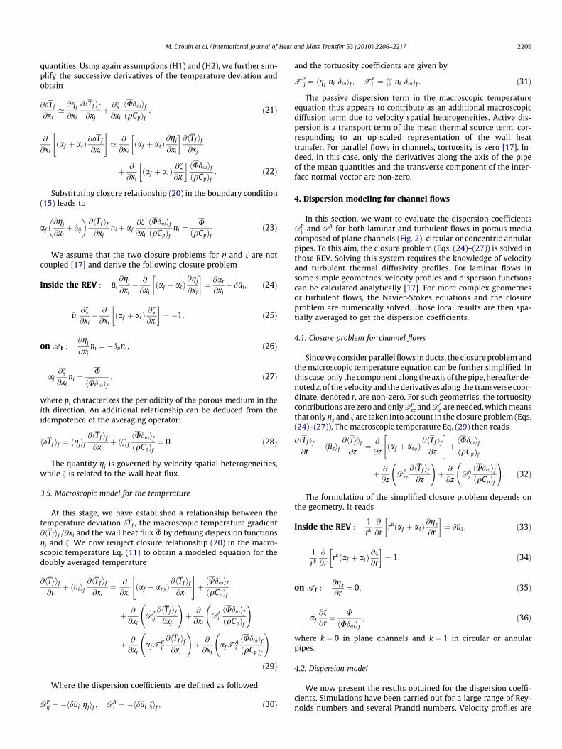
Fig. 1. Description of the averaging procedure in the single channel case.

Nomenclature

Af interface between solid and fluid phases ðm2ÞDA thermal active dispersion vector ðmÞDP thermal passive dispersion tensor ðm2 s�1ÞDh hydraulic diameter of the pores ðmÞfp friction coefficientni ith component of the interface normal vector, pointing

towards the solid phasePe Péclet number ðUDh=af ÞPr Prandtl number ðmf =af ÞPrt turbulent Prandtl number ðmt=atÞRe Reynolds number ðUDh=mf ÞTf fluid temperatureuf friction velocity ðms�1Þ

Greek symbolsaf thermal diffusivity of the fluid ðm2 s�1Þat turbulent thermal diffusivity ðm2 s�1Þat/ macroscopic turbulent thermal diffusivity ðm2 s�1Þdx Dirac delta function associated to the walls ðm�1Þ

DV representative elementary volume (REV) ðm3ÞDVf fluid volume included in the REV ðm3Þf active dispersion function ðsÞgj passive dispersion function ðmÞmf kinematic viscosity of the fluid ðm2 s�1Þmt turbulent kinematic viscosity ðm2 s�1Þq density of the fluid ðkgm�3ÞU wall heat flux

Other symbols� statistical average�0 fluctuation from the statistical averageh i volume averageh if fluid volume averaged� deviation from the fluid volume average�� dimensionless quantity�f fluid�w wall

M. Drouin et al. / International Journal of Heat and Mass Transfer 53 (2010) 2206–2217 2207

2. Averages

Since flows that are considered can be turbulent, a statisticalaverage operator, denoted ‘‘��”, is used to handle the pseudo-alea-tory character of turbulence. Since our aim is to develop a spatiallyhomogeneized modeling of these flows, we also need to apply aspatial filter. The spatial average operator used to derive a macro-scale model is denoted ‘‘ h�if ”. For each average, any quantity nmay be split into mean and fluctuating components as

n ¼ �nþ n0 ¼ hnif þ dn; ð1Þ

and one can write

n ¼ h�nif þ hn0if þ d�nþ dn0: ð2Þ

Pedras and De Lemos [16] proved that, in a strict mathematicalpoint of view, the order of application of statistical and spatialaverages is immaterial in regard to the mean flow quantities equa-tions. Nevertheless, the procedure based on the statistical averag-ing of the spatially averaged equations will require small eddiesto be modeled, as in Large Eddy Simulation. Therefore, applyingspatial filtering with a characteristic length scale larger than a porebefore statistical average would only allow the treatment of large-scale turbulence. This is questionable since the eddies larger thanthe scale of the porous structure are not likely to survive long en-ough to be detected [14]. Under these circumstances, followingPinson et al. [17], we choose to apply first the statistical average(Fig. 1). Thus Reynolds Averaged Navier-Stokes (RANS) modelscan be used to calculate temperature and velocity profiles withinsubchannels, and volume average may be used subsequently. Theproperties of both statistical and spatial average operators are re-called in Appendix A.

3. Formulation of the mean temperature equation

In this study, uncompressible and undilatable, single phaseflows in saturated, rigid porous media are considered. Fluid prop-erties (density, viscosity, heat capacity) and the porosity of themedium are assumed constant. A velocity no-slip condition atthe wall is imposed:

ui nijw ¼ 0: ð3Þ

Finally, we shall assume that thermal interactions with solidsreduce to an external forcing for the fluid temperature.

3.1. Averaged continuity equation

The instantaneous microscopic mass conservation equation isgiven by@ui

@xi¼ 0: ð4Þ

The no-slip boundary condition at walls and the properties ofthe spatial average operator allow us to write the doubly averagedmass conservation equation

@�ui

@xi

� �f

¼@h�uiif@xi

¼ 0: ð5Þ

3.2. Averaged fluid temperature equation

For constant fluid properties, the instantaneous microscopictemperature balance equation reads

@Tf

@tþ @ðTf uiÞ

@xi¼ @

@xiaf@Tf

@xi

� �; ð6Þ

2208 M. Drouin et al. / International Journal of Heat and Mass Transfer 53 (2010) 2206–2217

and the corresponding boundary condition on the wall Af is

af@Tf

@xini ¼

UðqCpÞf

on Af : ð7Þ

The use of the statistical average leads to the followingequations:

@Tf

@tþ @

@xið�uiTf Þ ¼ �

@

@xiu0iT

0f|{z}

turbulent heat flux

þ @

@xiaf@Tf

@xi

!; ð8Þ

af@Tf

@xini ¼

UðqCpÞf

on Af : ð9Þ

In Eq. (8), the turbulent heat flux is usually modeled with a firstgradient approximation

u0iT0f ¼ �at

@Tf

@xi; ð10Þ

where at is the turbulent thermal diffusivity. By analogy with themolecular Prandtl number, the turbulent Prandtl number is intro-duced: Prt ¼ mt

at. For flows in channels, Prt ¼ 0:9 is accurate enough

[13,10,1]. Applying volume average to (8), we obtain the doublyaveraged equation for the fluid temperature:

@hTf if@t

þ @

@xih�uiif hTf if ¼ �

@

@xiu0iT

0f

D Ef|fflfflfflffl{zfflfflfflffl}

macroscopicturbulentheat flux

þ @

@xiaf@hTf if@xi

!

þ haf@Tf

@xini dxi|fflfflfflfflfflfflfflfflfflfflfflffl{zfflfflfflfflfflfflfflfflfflfflfflffl}

wall heattransfer

þ @

@xihaf dTf nidxif|fflfflfflfflfflfflfflfflfflfflfflfflfflffl{zfflfflfflfflfflfflfflfflfflfflfflfflfflffl}tortuosity

� @

@xihd�ui dTf if|fflfflfflfflfflfflfflfflfflffl{zfflfflfflfflfflfflfflfflfflffl}

thermaldispersion

: ð11Þ

The macroscopic turbulent heat flux can be modeled by meansof a macroscopic turbulent thermal diffusivity at/ [14,16]:

u0iT0f

D Ef¼ �at/

@hTf if@xi

¼ � mt/

Prt

@hTf if@xi

: ð12Þ

Macroscopic turbulent viscosity models for flows in pipes aredetailed in Grégoire [7]. Thanks to Eq. (9), wall heat exchange reads

af@Tf

@xini dx

* +¼hUdxifðqCpÞf

: ð13Þ

Tortuosity and dispersion terms are typical of the porous med-ium approach. Dispersion is induced by a coupling between veloc-ity and temperature heterogeneities. Tortuosity results from theperturbation of diffusive fluxes in fluid due to the interactions withsolids. Let us notice that turbulent diffusivity does not induce tor-tuosity since it vanishes at walls. Those terms need to be modeled.

3.3. Temperature deviation equation

Tortuosity and dispersion terms in the doubly averaged temper-ature Eq. (11) involve the temperature deviation dTf . FollowingCarbonell and Whitaker [4], we derive the governing equation forthe temperature deviation in order to obtain a physical closurefor this problem. We subtract the macroscopic temperature Eq.

(11) from the statistically averaged temperature Eq. (8) to get thetemperature deviation equation and the boundary condition:

@dTf

@tþ @

@xið�uidTf Þ ¼

@

@xiaf@dTf

@xi

!þ @

@xiu0i T 0fD E

f� u0i T 0f

� �

þ @

@xihd�ui dTf if �

@

@xiðd�ui hTf if Þ ð14Þ

af@hTf if@xi

þ @dTf

@xi

!ni ¼

UðqCpÞf

on Af : ð15Þ

We now aim to simplify Eq. (14). Two major assumptions willcontribute to the dispersion model design.

H1: Separation of microscopic and macroscopic scales. Let usconsider a quantity n. We define a microscopic length scale ‘

and a macroscopic length scale L

1nkrnk ¼ O

1‘

� �;

1hnifkrhnif k ¼ O

1L

� �: ð16Þ

The assumption of scale separation reads L� ‘, and implies that

@dn@xi

�� @hnif

@xi

��: ð17Þ

H2: Weak unsteadiness of the temperature deviation

@dTf

@t

�� h�uiif

@dTf

@xi

��: ð18Þ

Since for the flows considered in this paper, unsteadiness is in-duced by variations of boundary conditions (mainly inlet condi-tions), this hypothesis is analogous to the separation betweenadvection and boundary conditions variation times scales. In otherwords, this assumption applies for non-pulsating heated flows inchannels. Let us notice that it is only used in order to simplify tem-perature deviation equation. It does not imply that averaged tem-perature shall be considered stationary.

Both assumptions (H1) and (H2) have been used to estimate theorder of magnitude of each contribution in Eq. (14) [17]. This,thanks to Eqs. (5), (10) and (12), leads to the simplified equationfor temperature deviation

�ui@dTf

@xi� @

@xiðaf þ atÞ

@dTf

@xi

" #¼ @at

@xi� d�ui

� �@hTf if@xi

�hU dxifðqCpÞf

:

ð19Þ

3.4. Closure problem

Unlike [15], we choose to model separately gradient and heatflux contributions. This choice is mainly motivated by the structureof source terms in the temperature deviation Eq. (19). Further-more, it is assessed by analytical developments and a priori teststhat, within both laminar and turbulent regimes, this closure accu-rately reproduce temperature profiles within channels. The follow-ing closure relationship is assumed

dTf ¼ gj

@hTf if@xj

þ fhUdxifðqCpÞf

þ w: ð20Þ

Carbonell and Whitaker [4] proved that w is zero for a spatiallyperiodic porous medium. The dispersion functions gj (homoge-neous to a length) and f (homogeneous to a time) are local


quantities. Using again assumptions (H1) and (H2), we further sim-plify the successive derivatives of the temperature deviation andobtain

@dTf

@xi’@gj

@xi

@hTf if@xj

þ @f@xi

hUdxifðqCpÞf

; ð21Þ

@

@xiðaf þ atÞ

@dTf

@xi

" #’ @

@xiðaf þ atÞ

@gj

@xi

@hTf if@xj

þ @

@xiðaf þ atÞ

@f@xi

hUdxifðqCpÞf

: ð22Þ

Substituting closure relationship (20) in the boundary condition(15) leads to

af@gj

@xiþ dij

� �@hTf if@xj

ni þ af@f@xi

hUdxifðqCpÞf

ni ¼U

ðqCpÞf: ð23Þ

We assume that the two closure problems for g and f are notcoupled [17] and derive the following closure problem

Inside the REV : �ui@gj

@xi� @

@xiðaf þ atÞ

@gj

@xi

¼ @at

@xj� d�ui; ð24Þ

�ui@f@xi� @

@xiðaf þ atÞ

@f@xi

¼ �1; ð25Þ

on Af :@gj

@xini ¼ �dijni; ð26Þ

af@f@xi

ni ¼U

hUdxif: ð27Þ

where pi characterizes the periodicity of the porous medium in theith direction. An additional relationship can be deduced from theidempotence of the averaging operator:

hdTf if ¼ hgjif@hTf if@xj

þ hfifhUdxifðqCpÞf

¼ 0: ð28Þ

The quantity gj is governed by velocity spatial heterogeneities,while f is related to the wall heat flux.

3.5. Macroscopic model for the temperature

At this stage, we have established a relationship between thetemperature deviation dTf , the macroscopic temperature gradient@hTf if =@xi and the wall heat flux U by defining dispersion functionsgj and f. We now reinject closure relationship (20) in the macro-scopic temperature Eq. (11) to obtain a modeled equation for thedoubly averaged temperature

@hTf if@t

þ h�uiif@hTf if@xi

¼ @

@xiðaf þ at/Þ

@hTf if@xi

" #þhUdxifðqCpÞf

þ @

@xiDP

ij

@hTf if@xj

!þ @

@xiDA

i

hUdxifðqCpÞf

!

þ @

@xiafT

Pij

@hTf if@xj

!þ @

@xiafT

Ai

hUdxifðqCpÞf

!;

ð29Þ

Where the dispersion coefficients are defined as followed

DPij ¼ �hd�ui gjif ; DA

i ¼ �hd�ui fif ; ð30Þ

and the tortuosity coefficients are given by

TPij ¼ hgj ni dxif ; TA

i ¼ hf ni dxif : ð31Þ

The passive dispersion term in the macroscopic temperatureequation thus appears to contribute as an additional macroscopicdiffusion term due to velocity spatial heterogeneities. Active dis-persion is a transport term of the mean thermal source term, cor-responding to an up-scaled representation of the wall heattransfer. For parallel flows in channels, tortuosity is zero [17]. In-deed, in this case, only the derivatives along the axis of the pipeof the mean quantities and the transverse component of the inter-face normal vector are non-zero.

4. Dispersion modeling for channel flows

In this section, we want to evaluate the dispersion coefficientsDP

ij and DAi for both laminar and turbulent flows in porous media

composed of plane channels (Fig. 2), circular or concentric annularpipes. To this aim, the closure problem (Eqs. (24)–(27)) is solved inthose REV. Solving this system requires the knowledge of velocityand turbulent thermal diffusivity profiles. For laminar flows insome simple geometries, velocity profiles and dispersion functionscan be calculated analytically [17]. For more complex geometriesor turbulent flows, the Navier-Stokes equations and the closureproblem are numerically solved. Those local results are then spa-tially averaged to get the dispersion coefficients.

4.1. Closure problem for channel flows

Since we consider parallel flows in ducts, the closure problem andthe macroscopic temperature equation can be further simplified. Inthis case, only the component along the axis of the pipe, hereafter de-noted z, of the velocity and the derivatives along the transverse coor-dinate, denoted r, are non-zero. For such geometries, the tortuositycontributions are zero and onlyDP

zz andDAz are needed, which means

that only gz and f are taken into account in the closure problem (Eqs.(24)–(27)). The macroscopic temperature Eq. (29) then reads

@hTf if@t

þ h�uzif@hTf if@z

¼ @

@zðaf þ at/Þ

@hTf if@z

" #þhUdxifðqCpÞf

þ @

@zDP

zz

@hTf if@z

!þ @

@zDA

z

hUdxifðqCpÞf

!: ð32Þ

The formulation of the simplified closure problem depends onthe geometry. It reads

Inside the REV :1rk

@

@rrkðaf þ atÞ

@gz

@r

¼ d�uz; ð33Þ

1rk

@

@rrkðaf þ atÞ

@f@r

¼ 1; ð34Þ

on Af :@gz

@r¼ 0; ð35Þ

af@f@r¼ U

hUdxif; ð36Þ

where k ¼ 0 in plane channels and k ¼ 1 in circular or annularpipes.

4.2. Dispersion model

We now present the results obtained for the dispersion coeffi-cients. Simulations have been carried out for a large range of Rey-nolds numbers and several Prandtl numbers. Velocity profiles are

Table 1Results for thermal dispersion coefficients: parallel flows in pipes (see Eqs. (38)–(41)).

Laminar regime

Planne channel Circular pipe

CPl

840 192

CAl

240 96

Concentric annular pipe

CPl 255:2� 341:5ðq2 � 2qÞ þ 1263:8½lnð1þ qÞ � q=2�

CAl 107:0þ 33:5ðq2 � 2qÞ þ 862:4½lnð1þ qÞ � q=2�

Asymptotic turbulent regime: Re!1

Planne channel Circular pipe

CPt

0.62 1.1

CAt

1.63 2.1

Concentric annular pipe

CPt 1:292� 0:362ðq2 � 2qÞ � 5:367½Inð1þ qÞ � q=2�

CAt 2:16� 0:715ðq2 � 2qÞ � 6:45½Inð1þ qÞ � q=2�

Fig. 2. Description of the porous media treated in this paper.


analytically calculated when possible, i.e. for laminar regime, or re-sult from RANS calculations for turbulent regime. To perform thelatter RANS simulations, we have implemented the low-Reynoldsnumber �k � �e Chien model [5] (Appendix B) in a CFD code. Sincewe consider parallel flows, velocity and thermal diffusivity profilesare calculated in 1D. The closure problem is discretized andnumerically solved in the section of the unit cell. Let us introducethe notations

DPzz ¼ afD

Pzz� ¼ �hd�uzgzif ; DA

z ¼ DhDAz� ¼ �hd�uzfif : ð37Þ

Once velocity and dispersion functions are determined, disper-sion coefficients DP

zz and DAz are calculated thanks to Eq. (37). With-

in laminar regime, our numerical results match analytical resultsas well as results from [15,17]:

DPzz� ¼ Pe2=CP

‘ for Re < ReL; ð38Þ

DAz� ¼ Pe=CA

‘ for Re < ReL; ð39Þ

where CP‘ and CA

‘ are constant and only depend on the geometry(see Table 1). The friction coefficient in laminar regime is fp ¼ al

Re

[3]. For very high Reynolds numbers, we find the same results asPinson et al. [17]:

DPzz� ¼ CP

t

ffiffiffiffifp

qPe for Re > 105; ð40Þ

DAz� ¼ CA

t for Re > 106; ð41Þ

where CPt and CA

t are constant and only depend on the geometry andthe friction coefficient in turbulent regime is fp ¼ atRe�bt [3]. The

values of CP‘ ;C

A‘ ;C

Pt and CA

t for each geometry are summarized in Ta-ble 1. In the case of a concentric annular pipe, the model constantsare expressed as functions of a geometrical parameter q, which isthe ratio between the inner radius r1 and the outer radius r2 ofthe pipe: q ¼ r1

r2.

For adiabatic flows through circular pipes, one can notice thatour passive dispersion model is consistent with the results pre-sented by Taylor [20] and Nakayama et al. [15]. Indeed they alsowrite DP

zz� ¼ CP

t

ffiffiffiffifp

pPe, with CP

t ¼ 1:78 in [20], CPt ¼ 2:475 in [15]

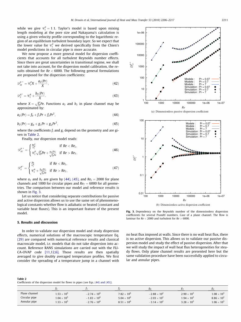
Fig. 3. Dependency on the Reynolds number of the dimensionless dispersioncoefficients for several Prandtl numbers. Case of a plane channel. The flow islaminar for Re < 2000 and turbulent for Re > 6000.


while we give CPt ¼ 1:1. Taylor’s model is based upon mixing

length modeling at the pore size and Nakayama’s calculation isusing a given velocity profile corresponding to the logarithmic re-gion of an equilibrium turbulent boundary layer. So we expect thatthe lower value for CP

t we derived specifically from the Chien’smodel predictions in circular pipe is more accurate.

We now propose a more general model for dispersion coeffi-cients that accounts for all turbulent Reynolds number effects.Since there are great uncertainties in transitional regime, we shallnot take into account, for the dispersion model calibration, the re-sults obtained for Re < 6000. The following general formulationsare proposed for the dispersion coefficients:

DPzz� ¼ CP

t X þ a2ðPrÞX

; ð42Þ

DAz� ¼ CA

t þb2ðPrÞ

X: ð43Þ

where X ¼ffiffiffiffifp

pPe. Functions a2 and b2 in plane channel may be

approximated by:

a2ðPrÞ ¼ f0 þ f1Pr þ f2Pr2; ð44Þ

b2ðPrÞ ¼ g0 þ g1Pr þ g2Pr2; ð45Þ

where the coefficients fi and gi depend on the geometry and are gi-ven in Table 2.

Finally, our dispersion model reads:

DPzz� ¼

Pe2

CP‘

if Re < ReL;

CPt

ffiffiffiffifp

pPeþ a2ðPrÞffiffiffi

fp

pPe

if Re > ReT ;

8<: ð46Þ

DAz� ¼

PeCA‘

if Re < ReL;

CAt þ

b2ðPrÞffiffiffifp

pPe

if Re > ReT ;

8<: ð47Þ

where a2 and b2 are given by (44), (45), and ReL ¼ 2000 for planechannels and 1000 for circular pipes and ReT ¼ 6000 for all geome-tries. The comparison between our model and reference results isshown in Fig. 3.

Let us notice that considering separate contributions for passiveand active dispersion allows us to use the same set of phenomeno-logical constants whether flow is adiabatic or heated (constant andvariable heat fluxes). This is an important feature of the presentmodel.

5. Results and discussion

In order to validate our dispersion model and study dispersioneffects, numerical solutions of the macroscopic temperature Eq.(29) are compared with numerical reference results and classicalmacroscale model, i.e. models that do not take dispersion into ac-count. Reference RANS simulations are carried out with the FLI-CA-OVAP code [11,12,6]. Those results are then spatiallyaveraged to give doubly averaged temperature profiles. We firstconsider the spreading of a temperature jump in a channel with

Table 2Coefficients of the dispersion model for flows in pipes (see Eqs. (44) and (45)).

f0 f1 f2

Plane channel 1:53� 105 �2:74� 106 7:82�Circular pipe 1:04� 105 �1:83� 106 5:04�Annular pipe 1:53� 105 �2:76� 106 8:51�

no heat flux imposed at walls. Since there is no wall heat flux, thereis no active dispersion. This allows us to validate our passive dis-persion model and study the effect of passive dispersion. After thatwe will study the impact of wall heat flux heterogeneities for stea-dy flows. Only plane channel results are presented here but thesame validation procedure have been successfully applied to circu-lar and annular pipes.

g0 g1 g2

106 �2:88� 102 2:90� 103 1:08� 103

106 �2:03� 102 1:94� 103 8:86� 102

106 �3:14� 102 3:28� 103 1:06� 103

Fig. 5. Evolution of a temperature jump: simulation results for laminar flow inplane channel, Pr ¼ 0:74;Re ¼ 175. Comparison between spatially averaged refer-ence RANS results (–), classical (---) and improved ðNÞ macroscale models.

Fig. 6. Evolution of a temperature jump: simulation results for intermediateturbulent flow in plane channel, case Pr ¼ 0:74;Re ¼ 76045. Comparison betweenspatially averaged reference RANS results (–), classical (-- -) and improved ðNÞmacroscale models.


5.1. Spreading of a temperature jump

5.1.1. Validation of the passive dispersion modelIn this section, we study the evolution of a temperature jump

with respect to the time (Fig. 4). The fluid flows at constant massflow rate along the axis of the pipe, denoted z. The pipe isL ¼ 60Dh long. Initially, the fluid temperature is uniform over thepipe: Tðz; t ¼ 0Þ ¼ T0. The fluid temperature at the inlet, i.e. inz ¼ 0, is uniform over the section. At t ¼ t0, we increase the inlettemperature so that Tðz ¼ 0; t P t0Þ ¼ Te > T0 Since adiabatic con-ditions are imposed at walls, there is no active dispersion. Lets usnotice that, near the channel inlet, assumption (H1) is not valid.Our model can still be used because the temperature jump spreadsrapidly, which means that assumption (H1) is true everywhere, ex-cept in a small zone nearby the channel inlet. Figs. 5–7 present thecomparison between bulk temperature, spatially averaged temper-ature calculated with the macroscale model described in Section 4and spatial average of fine scale reference simulations for Pr ¼ 0:74and Re ¼ 175; 7:6� 104 and 1:14� 106. Most industrial thermalhydraulic codes used for nuclear purpose [2,8] do not account fordispersion. This might lead to strongly underestimate the spread-ing of temperature jumps. For the cases here considered, the meantemperature increases earlier and decreases later than what classi-cal models predict. Agreement between fine scale simulations andour improved macroscale model is excellent.

5.1.2. Comparison between dispersion and diffusionFor adiabatic flows in channels, the macroscopic temperature

equation reads

@hTf if@t

þ h�uzif@hTf if@z

¼ @

@zðaf þ at/ þDP

zzÞ|fflfflfflfflfflfflfflfflfflfflfflfflffl{zfflfflfflfflfflfflfflfflfflfflfflfflffl}ae

@hTf if@z

264

375: ð48Þ

Lets us first consider laminar regime. Macroscopic turbulentthermal diffusivity is then zero, and one can write

ae ¼ af 1þDPzz�� ¼ af 1þ Pe2

CP‘

!: ð49Þ

Consequently

If Pe�ffiffiffiffiffiffiCP‘

q, then DP

zz � af and molecular diffusion rules over

passive dispersion;

If Pe�ffiffiffiffiffiffiCP‘

q, then DP

zz � af and passive dispersion rules over

molecular diffusion.

From these we see that passive dispersion rapidly predominatesover molecular diffusion for increasing Péclet numbers.

Now within turbulent regime, Pinson et al. [17] propose

at/ ¼ afCa

ffiffiffiffifp

qPe; ð50Þ

with Ca 10�2. Using (40) for high Reynolds numbers, effectivethermal diffusivity may be written

Fig. 4. Description of the dispersion model test-case:

ae ¼ af 1þ Ca þ CPt

� � ffiffiffiffifp

qPe

ð51Þ

evolution of a temperature jump along the time.

Fig. 7. Evolution of a temperature jump: simulation results for asymptoticturbulent flow in plane channel, Pr ¼ 0:74;Re ¼ 1140684. Comparison betweenspatially averaged reference RANS results (–), classical (---) and improved ðNÞmacroscale models.


Moreover, for turbulent flows,ffiffiffiffifp

pPe� 1, which means that

molecular diffusion is negligible with respect to turbulent thermaldiffusivity and passive dispersion. In addition, we have seen in Sec-tion 4 that 0:1 6 CP

t 6 1. Hence CPt � Ca and passive dispersion

strongly predominates over turbulent thermal diffusivity.Finally, for the range of Péclet numbers here considered, passive

dispersion always predominates over diffusion. Thus, neglectingdispersion would lead to strongly underestimate the spreading oftemperature jumps.

Fig. 8. Influence of the Prandtl number on the spreading of temperature jump:focus on the temporal evolution of the mean temperature calculated at z ¼ 50Dh fora laminar flow in plane channel.

5.1.3. Influence of the Prandtl numberFisrt of all, we focus on laminar regime, we have seen in Sec-

tion 5.1.2 that ae in Eq. (48) can be written

ae ¼ af 1þDPzz�� ¼ af 1þ Pe2

CP‘

!¼ mf

1Prþ Re2

CP‘

Pr

!: ð52Þ

One can then write

@ae

@Pr¼ mf

Pr2

Pe2

CP‘

� 1

!: ð53Þ

Two different behaviours may be observed, depending on thevalue of the Prandtl number:

If Pe2 > CP‘ , effective thermal diffusivity increases with Pr;

Else this quantity decreases for increasing Prandtl numbers.

Let us illustrate this observation thanks to an example. For asteady flow in a plane channel with Re ¼ 175, Eq. (53) cancels for

Pe ¼ffiffiffiffiffiffiCP‘

q() Pr ¼ 0:166: ð54Þ

Mean temperature profiles are calculated for Pr ¼ 0:1;

0:15; 0:2; 0:3. Fig. 8 shows that effective thermal diffusivity in-creases between Pr ¼ 0:1 and Pr ¼ 0:15, and decreases betweenPr ¼ 0:2 and Pr ¼ 0:3. This result confirm our analysis.

For very high Reynolds numbers, we have, with Eq. (40),

ae ¼ af 1þ Ca þ CPt


qPe

¼ mf

1Prþ Ca þ CP

t


qRe

ð55Þ

and

@ae

@Pr¼ � mf

Pr2 : ð56Þ

Consequently, effective thermal diffusivity decreases forincreasing Prandtl numbers.

5.2. Impact of wall heat flux nonuniformity

5.2.1. Validation of the active dispersion modelLet us now study the case of a steady flow in a pipe with piece-

wise linear heat flux imposed at the wall (Fig. 9). The fluid flowsalong the axis of the pipe, denoted z. The pipe is L ¼ 60Dh long.

Fig. 9. Description of the dispersion model test-case: steady flow in the presence of wall heat flux heterogeneities. Wall heat flux is given by Eq. (57).


The fluid temperture in z ¼ 0 is uniform over the section :Tðz ¼ 0Þ ¼ T0. The wall heat flux is given by (see also Fig. 9)

U ¼

0 if z < 10Dh or z > 50Dh;

Umaxz�10Dh

20Dhif 10Dh < z < 30Dh;

Umax50Dh�z

20Dhif 30Dh < z < 50Dh;

8>><>>: ð57Þ

Fig. 10. Simulation results: laminar steady flow in plane channel in the presence ofwall heat flux heterogeneities, Pr ¼ 0:74;Re ¼ 175. Comparison between spatiallyaveraged reference RANS results (–), classical (---) and improved ðNÞ macroscalemodels. DT is defined by: DT ¼ hTf if ðz ¼ zoutletÞ � hTf if ðz ¼ zinletÞ.

For each geometry, three Reynolds numbers are studied, in or-der to validate our dispersion model in the three regimes: laminar,intermediate and asymptotic. Simulation results in plane channeland discrepancy curves for Pr ¼ 0:74 and Re ¼ 175;7:6� 104 and1:14� 106 are shown in Figs. 10–12. One can notice that account-

Fig. 11. Simulation results: intermediate turbulent steady flow in plane channel inthe presence of wall heat flux heterogeneities, Pr ¼ 0:74;Re ¼ 76045. Comparisonbetween spatially averaged reference RANS results (–), classical (---) and improvedðNÞ macroscale models. DT is defined by: DT ¼ hTf if ðz ¼ zoutletÞ � hTf if ðz ¼ zinletÞ.


ing for dispersion strongly improves macroscale simulation results.Indeed, discrepancies between reference results and macroscalemodels are 5–10 times smaller when dispersion is taken intoaccount.

5.2.2. Comparison between active and passive dispersionWe now want evaluate the relative importance of active disper-

sion and passive dispersion in the case of a steady flow with non-uniform wall heat flux and without temperature jumps. We recallthat, in a channel flow, the active dispersion term is

Active dispersion ¼ 4DAz

ðqCpÞf Dh

@U@z

; ð58Þ

and the passive dispersion term may be approximated by

Fig. 12. Simulation results: asymptotic turbulent steady flow in plane channel inthe presence of wall heat flux heterogeneities, Pr ¼ 0:74;Re ¼ 1140684. Compar-ison between spatially averaged reference RANS results (–), classical (---) andimproved ðNÞ macroscale models. DT is defined by: DT ¼ hTf if ðz ¼ zoutletÞ�hTf if ðz ¼ zinletÞ.

Passive dispersion ¼ @

@zDP

zz

@hTf if@z

" #

DPzz �

4ðqCpÞf UDh

� @U@z

: ð59Þ

This, using Eqs. (38)–(41), leads to

Passive dispersionActive dispersion

CA‘

CP‘

if Re < 2� 103;

CPt

ffiffiffifppCA

tif Re > 106:

8><>: ð60Þ

In other words, within laminar regimes, the ratio between ac-tive and passive dispersion is constant and only depends on thegeometry. Its value is 2

7 in plane channels and 12 in circular pipes.

For turbulent steady flows, this ratio is small, and active dispersionstrongly predominates over passive dispersion. Results obtained inplane channel for Re ¼ 76045 and Pr ¼ 0:74 (Fig. 13) illustrate ourestimations.

6. Nonuniform wall heat flux and temperature burst

In order to evaluate simultaneously passive and active disper-sion effects, we have simulated the evolution of a temperatureburst in a plane channel with nonuniform wall heat flux. The fol-lowing parameters are chosen Re ¼ 2� 104; Pr ¼ 0:2; L ¼ 1:43 m;

Dh ¼ 10 mm;ðqCpÞf ¼ 1000 Jm�3 K�1; h�uif ¼ 52 ms�1.The following wall heat flux is imposed

U ¼ Umax cos p zL� p

2

� h i; Umax ¼ 1820 Wm�2: ð61Þ

Initially, the mean temperature is supposed to be given by stea-dy solutions of classical and improved macroscale models, respec-tively denoted Tclassical

1 and Timproved1 . At time t ¼ t0, we impose the

following mean temperature profile:

Twðt ¼ t0; zÞ ¼ Tw1ðzÞ þ DTðzÞ; with w

¼ classical or improved; ð62Þ

where:

DTðzÞ ¼ h if z1i < z < z2

i ;

0 elsewhere:

(ð63Þ

Fig. 13. Turbulent steady flow in plane channel in the presence of wall heat fluxheterogeneities: comparison between active and passive dispersion.


and:

h ¼ 10�C; z1i ¼ Dh; z2

i ¼ 11Dh: ð64Þ

Results given by classical and improved macroscale models arecompared in Fig. 14. The temperature burst collapses because ofpassive dispersion while active dispersion perturbates the steadysolution on the problem. Passive dispersion predominates untilthe temperature jump vanishes and a steady regime is achieved.We then find similar results as in Section 5.2.

7. Conclusion

In this paper, a macroscopic model for laminar and turbulentflows in heat exchangers has been proposed. Use have been madeof a statistical average and a spatial filter to derive the governingequation of the mean flow temperature. The double averaging pro-cedure put forward dispersion terms. Up-scaling effects split intotwo contributions: a first one due to the velocity spatial heteroge-neities, called passive dispersion, and a second one related to thewall heat flux, called active dispersion. A closure problem has been

240

245

250

255

260

265

0 20 40 60 80 100 120 140

With dispersionWithout dispersion

Fig. 14. Evolution of a temperature burst in a plane channel with nonuniform wallheat flux. Temperature burst is imposed a the inlet at t ¼ t0. It is then advectedthrough the channel.

derived by representing the temperature spatial deviation as afunction of the macroscopic temperature gradient and the aver-aged wall heat flux. A practical and accurate model has been pro-posed for dispersion in pipes: dispersion coefficients have beenexpressed as functions of the Péclet number and the friction coef-ficient and the same constants apply whether flow is adiabatic, orwith constant or variable heat fluxes. Results given by a macroscalemodel with those dispersion terms have been compared withnumerical reference results and classical macroscale model.Noticeably improved results have been obtained for steady andtransient flows in plane channel, circular and concentric annularpipes. Simulations highlighted the importance of dispersion effectsfor heated flows in pipes in the presence of wall heat flux hetroge-neities or temperature jumps.

Appendix A. Properties of averaging operators

A.1. Statistical average

We first introduce the statistical decomposition commonlyused in turbulence modeling. Any physical quantity n can be writ-ten as the sum of its statistical average and a fluctuation:

n ¼ �nþ n0: ð65Þ

The statistical average is linear, idempotent and commutes withthe differential operators.

A.2. Spatial average

Following Taylor [20] and Whitaker [21], we use the method ofvolume averaging. This up-scaling process is linked to the defini-tion of a spatial average operator and a fluid characteristic func-tion. In this study, use have been made of a volume averagingoperator corresponding to a spatial integration over a REV [16]DV . For any quantity n, we have

hniðx; tÞ ¼ 1DVðxÞ

ZVðxÞ

nðx; tÞdV ; ð66Þ

where DVðxÞ, the volume of the REV, depends on the properties ofthe porous medium. For a spatially periodic porous medium,DVðxÞ represents a unit cell of the solid matrix [18,19]. If variationslength scales of the macroscopic quantities are large with respect tothe filter size, then spatial average can be assumed idempotent[4,19].

The fluid characteristic function vf is equal to one in the fluidphase and zero elsewhere. Any physical quantity n can be written

n ¼ hnif þ dn: ð67Þ

This operator is clearly linear, due to its integral formulation.The spatial average does not commute with the space-time differ-ential operators. Howes and Whitaker [9] showed the followingderivation rules:

/@n@xi

� �f¼@/hnif@xi

þ /hn ni dxif ¼ /@hnif@xiþ /hdn ni dxif ; ð68Þ

/d@n@xi

� �¼ /

@dn@xi� /hdn ni dxif ; ð69Þ

/@n@t

� �f¼@/hnif@t

þ /hn xi ni dxif ¼ /@hnif@tþ /hdn xi ni dxif ;

ð70Þ

/d@n@t

� �¼ /

@dn@t� /hdn xi ni dxif ; ð71Þ


where x is the fluid-solid interface velocity, n the interface normalvector pointing towards the solid phase and dx the Dirac delta func-tion associated to the interface.

Appendix B. �k� �e Chien model

A general form for low Reynolds number �k� �e models is

mt ¼ Clfl�k2=�e; ð72Þ

@�k@tþ �uj

@�k@xj¼ �u0iu

0j

@�ui

@xjþ @

@xjmf þ

mt

rk

� �@�k@xj

" #� �e� �ep; ð73Þ

@�e@tþ �uj

@�e@xj¼�C�1 f1

�e�k

u0iu0j

@�ui

@xjþ @

@xj

mt

r�þmf

� �@�e@xj

�C�2 f2

�e2

�k�Ep:

ð74Þ

where f1; f2 et fl are dumping functions, and �ep et Ep additional dis-sipation terms. Chien [5] gives for the functions and coefficients ofthe model

fl ¼ 1� expð�0:0115yþÞ; f 1 ¼ 1 f 2 ¼ 1� 0:22 expð�Re2t =36Þ;

�ep ¼ 2mf

�ky2

w

!; Ep ¼ 2mf

�ey2

w

� �expð�yþ=2Þ; �e ¼ 0 on the wall;

Cl ¼ 0:09; C�1 ¼ 1:35; C�2 ¼ 1:8; rk ¼ 1; r� ¼ 1:3:

ð75Þ

References

[1] Y. Benarafa, Application du couplage RANS/LES aux écoulements à hautnombre de Reynolds de l’industrie nucléaire, PhD Thesis, Université Paris VI,Paris, France, 2005.

[2] D. Bestion, The physical closure laws in the CATHARE code, Nucl. Eng. Design124 (3) (1990) 229–245.

[3] I.E. Idel’cik, Memento des pertes de charge, Eyrolles (1969).[4] R.G. Carbonell, S. Whitaker, Dispersion in pulsed systems – II: theoretical

developments for passive dispersion in porous media, Chem. Eng. Sci. 38 (11)(1983) 1795–1802.

[5] K.Y. Chien, Prediction of channel and boundary layer flows with a low-Reynolds number turbulence model, AIAA J. 20 (1) (1982) 33–38.

[6] M. Drouin, Implémentation et validation de modèles de turbulence dans lecode hydrodynamique FLICA-OVAP, Technical Report, SFME/LETR/07-040/A,CEA, 2007.

[7] O. Grégoire, Remarques sur la turbulence permettant de retrouverquantitativement ou qualitativement un certain nombre de résultatsexpérimentaux : le point de vue en 2003, Technical Report, SFME/LETR/RT/03-013/A, CEA, 2003.

[8] O. Grégoire, E. Royer, J.-P. Magnaud, L. Roux and X. Masson, HORUS3D/TH:thermal hydraulic modelling of the Jules Horowitz Reactor core with FLICA4,in: Proceedings of the Seventh ICAPP Conference (Nice), 2007.

[9] F.A. Howes, S. Whitaker, The spatial averaging theorem revisited, Chem. Eng.Sci. 40 (8) (1985) 1387–1392.

[10] H. Kawamura, K. Ohsaka, H. Abe, K. Yamamoto, DNS of turbulent heat transferin channel flow with low to medium-high Prandtl number fluid, Int. J. HeatFluid Flow 19 (1998) 482–491.

[11] A. Kumbaro, V. Seignole, Two-phase flow computing with the OVAP code, in:Proceedings of Workshop Trend in Numerical ans Physical Modeling forMultiphase Flows (Cargese), 2001.

[12] A. Kumbaro, I. Toumi, V. Seignole, Numerical modeling of two-phase flowsusing advanced two fluid systems, in: Proceedings of ICONE 10 (Arlington,Virgina, USA), 2002.

[13] S. Lyons, T. Hanratty, J. Mc Laughlin, DNS of passive heat transfer in a turbulentflow, Int. J. Heat Mass Transfer 34 (4/5) (1991) 1149–1161.

[14] A. Nakayama, F. Kuwahara, A macroscale turbulence model for flows in aporous medium, J. Fluids Eng. 121 (1999) 427–433.

[15] A. Nakayama, F. Kuwahara, Y. Kodama, An equation for thermal dispersion fluxtransport and its mathematical modelling for heat and fluid flow in a porousmedium, J. Fluid Mach. 563 (2006) 81–96.

[16] M.H.J. Pedras, M.J.S. De Lemos, Macroscopic turbulence modeling forincompressible flow through undeformable porous media, Int. J. Heat MassTransfer 44 (2001) 1081–1093.

[17] F. Pinson, O. Grégoire, M. Quintard, M. Prat, O. Simonin, Modeling of turbulentheat transfer and thermal dispersion for flows in flat plate heat exchangers,Int. J. Heat Mass Transfer 50 (2007) 1500–1515.

[18] M. Quintard, S. Whitaker, Transport in ordered and disordered porous media I:the cellular average and the use of weighting functions, Transport Porous Med14 (1994) 163–177.

[19] M. Quintard, S. Whitaker, Transport in ordered and disordered porous mediaII: generalized volume averaging, Transport Porous Med 14 (1994) 179–206.

[20] G. Taylor, Dispersion of solute matter in solvent flowing slowly through a tube,Proc. Roy. Soc. Lond. A 219 (1953) 183–203.

[21] S. Whitaker, Diffusion and dispersion in porous media, AIChE 13 (3) (1967)420–427.

[22] S. Whitaker, Theory and Applications of Transport in Porous Media: theMethod of Volume Averaging, Kluwer Academic Publishers, 1999.

macroscopic modeling of thermal dispersion for turbulent flows in channels

Documents