macro-cell and module placement by genetic adaptive...

49

Macro-cell and module placement by genetic adaptive search with bitmap-represented chromosome

Heming Chan i, p. Mazumder and K. Shahookar Department of Electrical Engineering and Computer Science, The University of Michigan, Ann Arbor, MI 48109, USA

Abstract. The genetic algorithm has been applied to the VLSI module placement problem. This algorithm is an iterative, evolutional approach. A placement configuration is represented by a set of primitive features such as location and orientation, and the features are arranged in the form of a two-dimensional bitmap chromosome. The representation is flexible, and can handle arbitrarily shaped cells, and pads, and is applicable to the placement of macro cells, and gate arrays. Three new versions of genetic operators, namely, crossover, inversion and mutation, are used to explore the solution space. Crossover creates new configurations by combining attributes from a pair of existing configurations. This feature passing scheme constitutes the primary difference between our genetic approach and the other traditional searching techniques. Inversion enables more uniform inheritance of features from one generation to the next, and mutation prevents the algorithm from getting trapped at local optima. We have pointed out that the bitmap representation enables the algorithm to divide the entire solution space into a set of feature-equivalent classes, or schemata where each class contains a set of solutions with common physical attributes. We show that the genetic algorithm adaptively biases the search based on the past observed fitness of the schemata. We also demonstrated the power of the genetic algorithm experimentally for macro cell placement, and obtained satisfactory results.

Keywords. VLSI, placement, layout, macro cell, floorplanning, integrated circuit (IC) design, genetic algorithm, adaptive search, combinatorial optimization.

I. Introduction

Predesigned and highly optimized digital and analog circuit modules or macro blocks are frequently used in custom VLSI circuits. The placement of arbitrarily

i Currently at Mentor Graphics Corp., Wilsonville, OR, USA.

Elsevier INTEGRATION, the VLSI journal 12 (/991) 49-77

0167-9260/91/$03.50 © 1991 - Elsevier Science Publishers B.V. All rights reserved

50 H. Chan et aL / Module placement by genetic adaptive search

s h a p e d and sized cells has, t he r e fo re , b e c o m e increas ingly i m p o r t a n t in V L S I layout a u t o m a t i o n . In this p a p e r , the p l a c e m e n t of func t iona l m o d u l e s wi th var ious shapes , sizes and o r i en t a t i ons is cons ide red , and it is shown tha t an adap t ive op t imiza t i on t echn ique , the G e n e t i c A lgo r i t hm, can p rov ide a high qual i ty p l a c e m e n t in a r e a s o n a b l e run t ime. T h e object ive is to min imize the to ta l wire l eng th of the i n t e r connec t i on s and to p lace the cells such tha t the chip a r ea is min imized . M a n y heur i s t ic s t ra teg ies for m a c r o cell p l a c e m e n t b a s e d on i te ra t ive i m p r o v e m e n t have b e e n r e p o r t e d recent ly . E x a m p l e s a re fo r ce -d i r ec t ed p l a c e m e n t [1,2,28], ra in-cut p l a c e m e n t [3,4,29], s imu la t ed a n n e a l i n g [5-7] , and

pass ive resis t ive op t imiza t i on [8]. S imu la t ed annea l ing is one of the la tes t t echn iques be ing used for cell p l a c e m e n t . T h e heur is t ic o f s i m u l a t e d a n n e a l i n g is b a s e d on stat is t ical mechan ics . T h e bas ic p r o c e d u r e is to accep t all m o v e s which resul t in a d e c r e a s e in cost, and to accep t those moves which resul t in an

Heming Chan received the BS degree in Electrical Engineering from National Chiao Tung University, Taiwan and MS degree in Electrical Engineering from the University of Michigan, Ann Arbor. He is pursuing the PhD degree in E.E. at the University of Michigan, and is currently working with the IC group, Mentor Graphics Corp., Wilsonville, OR. His research interests include CAD for VLSI, machine learning and computer vision.

Khushro Shahookar was born in Karachi, Pakistan on September 10, 1962. He received the BSc degree in Electrical Engineering from the University of Engineering and Technology, Lahore, Pakistan in 1986, and the MS degree in Electrical Engineering from the University of Michigan, Ann Arbor in 1989, where he is currently a PhD student. His main interests are VLSI fabrication technology and automated VLSI layout algorithms.

Pinaki Mazumder (S'84-M'87) received the BSEE degree from the Indian Institute of Science in 1976, the MSc degree in Computer Science from the University of Alberta, Canada in 1985, and the PhD degree in Electrical and Computer Engineering from the University of Illinois in 1987. Presently he is working as an Asgistant Professor at the Department of Electrical Engineering and Computer Science of the University of Michigan, Ann Arbor. Prior to this he worked two years as a research assistant at the Coordinated Science Laboratory, University of Illinois, and over six years at the Bharat Electronics Ltd. (a collaborator of RCA) in the area of integrated circuit design and applications. During the summers of 1985 and 1986, he worked as a Member of Technical Staff in the Computer-Aided Design Group of AT&T Bell Laboratories. His

research interests include VLSI testing, computer-aided design, parallel architectures, and neural networks. He is the recipient of Digital's Incentives for Excellence Award, NSF Research Initiation Award, and Bell Northern Research Laboratory Faculty Award,

Dr. Mazumder is a member of IEEE, Sigma Xi, Phi Kappa Phi and ACM SIGDA.

H. Chan et aL / Module placement by genetic adaptiue search 51

increase in cost with a Boltzmann acceptance probability that monotonically decreases with time. It yields good placement solutions [5,6]. However, simulated annealing is a very time-consuming process. Moreover, the efficiency of simulated annealing also depends strongly on the annealing schedule. The general problem of finding an optimal cooling schedule for a given netlist is still open for research. Although much effort has been spent to parallelize simulated annealing [9,10], it is known to be a serial algorithm which cannot be efficiently parallelized in the distributed workstation environment.

This paper applies the genetic algorithm to macro cell placement for VLSI design. The idea of using biological evolution has been applied recently to standard cell placement [11,12,30]. In their approach, a list of cells is used as a chromosome to represent the linear ordering of cells. However, their approach is not suitable for macro cell placement where cells of arbitrary sizes and shapes have to be placed at any location inside a frame. Moreover, the genetic operations defined in their approach are informally heuristic, and no analytical model exists. In this paper, a new bitmap chromosomal representation is proposed for representing cells that can be placed at any arbitrary locations and orientations inside a frame. This representation is flexible enough to handle various aspects of cell placement under different design methodologies such as customized macro cell, standard cell and gate array design methods. The placement problem is first mapped to a function optimization problem. Instead of using the traditional bit-string genetic representation [13] the possible solution is encoded in the form of a chromosome with a set of genes arranged in a two-dimensional array. This two-dimensional representation benefits from a divide-and-conquer methodology, which reduces the amount of computation time, as compared to the conventional bit-string representation. Three genetic operators, namely, crossover, inversion and mutation are then applied to a set of chromosomes called population. Crossover is used primarily to generate new configurations by combining physical attributes (genes) from a pair of chromosomes existing in the current population. Inversion is used to decouple the correlation among genes so that genes can be passed to their offspring with less dependence on their relative grouping, and mutation is used to increase the diversity of the genes in a population. The concept of feature-equivalent classes, or schemata, provides an insight into the powerful adaptive property of the algorithm. We show that the algorithm automatically divides the solution space into subsets called schemata on the basis of the physical features and adaptively selects possible configurations from classes that have good estimated quality.

This paper is organized as follows. Section 2 introduces the concept of the genetic algorithm and the criteria for applying it to engineering problems. Section 3 describes how the macro cell placement problem can be mapped to the function optimization problem and how the chromosomal representation and the genetic operators are constructed. Section 4 discusses the adaptive strategy of the algorithm. Experiments and implementation are reported in Section 5.

52 H. Chan et al. / Module placement by genetic adaptive search

2. The concept of the genetic algorithm

The genetic algorithm (GA), developed at the University of Michigan by Holland [13] and his colleagues [14,26] is a search strategy based on the mechanics of natural selection and natural reproduction in a biological system [15,16]. It represents complicated systems by decomposing them into their fundamental components, and uses randomized information exchange operations to guide efficient, self-adaptive searching. As a result, a chromosome that survives under the genetic algorithm's survival o f the fittest strategy represents a globally optimal (or near-optimal) solution. The genetic algorithm differs from the other stochastic search techniques by being able to encode and exploit past information efficiently during a search. This learning ability provides the genetic algorithm with a guiding capability for searching efficiently through a complex multi-dimensional search space.

A number of biologists [17-19] and AI researchers [20-22] studied the searching capability of the genetic algorithm. DeJong [14] and Brindle [27] undertook a systematic study of the genetic algorithm in the context of function optimization. These in-depth studies show that the genetic algorithm exploits information about the environment in an attempt to shorten the duration and improve the efficiency of a search. This feedback information consists of the fitness or performance of the solutions, and the stored information regarding solutions already investigated. This stored information allows the GA to learn from the history of the past search, and, therefore, it is adaptive in seeking new searching paths. Many optimization and searching algorithms, such as the hill-climbing, gradient-based methods and simulated annealing, fail to store and exploit past experience and simply enumerate points in a search space, in a predetermined or random order.

The concept of schemata provides an insight into the powerful adaptive property of the genetic algorithm. A schema is a subset of chromosomes with some common values on the selected attributes. Thus, a schema denotes a class of structures, where the elements have some attributes in common. The genetic operators search through the space of schemata in an attempt to find combinations of attributes contributing to the structure's fitness. This searching in the space of schemata marks one of the primary differences between genetic adaptive search and the other searching techniques. A single evaluation of a new structure refines the estimated fitness of all schemata represented by the structure. The ability to process enormous numbers of schemata, by manipulat- ing a small set of chromosomes, is called intrinsic parallelism. This parallelism marks another powerful property unique to the genetic algorithm. A simple version of the genetic algorithm is shown below:

Procedure GENETIC ALGORITHM Step 1: Randomly form a population of chromosomes. Step 2: Select pairs of chromosomes as parents, chromosomes with higher

fitness are more likely to be selected.

H. Chan et al. / Module placement by genetic adaptive search 53

Step 3: Apply genetic operators to the pairs to create offspring. Step 4: Replace the least lit chromosome with offspring. Go to step 2.

END Procedure

In order to fully exploit the efficiency of the genetic search, certain criteria should be met while designing the genetic algorithm for specific engineering applications. These criteria are explained in detail by Holland [13] and Goldberg [23], and are briefly summarized as follows: • The cardinality of the alphabet used to represent a gene should be as small as

possible. • The genetic operators should produce legal solutions in each generation. • The algorithm should be adaptive in nature.

In the next section, we will show how the proposed bit-map chromosomal representation and genetic operators are designed to meet the above three criteria.

3. GAMPmA genetic approach to macro cell placement

3.1. Function optimization formulation

The Cell Placement Problem consists of placing a set of L predefined circuit modules on a chip such that a certain objective function is minimized. We show that the cell placement problem is equivalent to the problem of optimizing a one-dimensional function. We start by formulating the mathematical entities involved. Let R = {1, 2, 3 , . . . , L} be an index set of the blocks to be placed; let C be the set of all possible placement configurations, or the configuration space. A block placement configuration c ~ C can be completely represented by three L-dimensional vectors, namely, the x-coordinate vector x, the y-coordinate vector y and the orientation transformation vector o. For each i ~ B, the ith component of x (y) stands for the x (y) coordinates of the ith cell in a configuration. The ith component of o denotes one of the eight permissible Manhattan orientations of the ith cell. The three-bit codes for the eight Manhattan transforms are fixed as shown in Fig. 1.

In this paper, we have adopted the semi-perimeter wire length as the quality of a placement configuration, since it gives a reasonable indication as to how expensive it is to construct the detailed routing of the wires after the blocks have been placed [5,6,9]. The blocks are allowed to overlap with one another as an intermediate solution to the final configuration. Penalties for overlapping area among blocks and the total area of the chips are also used as criteria for optimization. We assume that the routing area for each cell has been included within the perimeter of the cell itself. The problem to solve is, therefore, to pack the cells as tightly as possible, and to minimize the estimated wire length.


Input L shaped cell

(a)

0 0 0 0 0 1 0 1 0 OI 1 I 0 0 I 0 1 I I 0 I I 1

8 Manhattan transforms

(D)

Fig. 1. (a) An input L-shaped cell; (b) eight Manhat tan orientations and their binary codes.

Hence, the cost of a placement configuration c E C is defined as the following weighted sum of four factors [5]

Cost(c) = K I C 1 + K b C b + K o C o + K a C a.

Here, C~ is the estimated total wire length, where the length of a net is estimated by computing the half-perimeter of the bounding box enclosing all the pins connected to the net [6]. C b is the bounding area, which is the area of the smallest rectangle enclosing all the cells, C o is a penalty function for the total overlapping area between cells. C a is the outside area, i.e. the area of cells lying outside given bounds. While the bounding area term minimizes the actual bounding area of the chip, the outside area term ensures that entire placement lies within the given bounding area, and is of the right aspect ratio. The overlap and outside area terms have to be zero at the end of the algorithm, to achieve a feasible placement. Kb, Kl, Ko, and K a are non-negative weights that are experimentally adjusted. The fitness f ( c ) of a placement configuration c is defined as the weighted reciprocal of its cost, that is,

K

f ( c ) = C o s t ( c ) '

where K is a constant. Let nx, ny, n o be the number of binary bits used to represent the x-coordinate, y-coordinate and orientation of a module, respectively. Let rn = nx + ny + n o be the resolution of a placement problem, and let T be a transformation defined as

T ( c ) = T ( x , y , o ) = x 1 : X2 " " " XL : Y l : YZ " " " YL :O1 :O2 " "" OL,

where x i, Yi, oi are the ith components of the corresponding vectors represented in a binary form, and: (the colon mark) denotes concatenation. The range of T is a set of binary strings S of length L × m. Hence for c ~ C and s ~ S, the fitness of a configuration is related to the string as below:

f ( c ) = f ( T - l ( s ) ) = f * ( s ) .


Thus, the cell placement problem can be conceived as a function optimization problem, which can be stated as:

Given the cells and the net list of a placement problem, find a binary string s in S that maximizes the function f*(s) .

Observation 1. For sufficiently large m, the cell placement problem is equivalent to the one-dimensional function optimization problem.

This is a direct consequence of the fact that T is a one-to-one mapping. In this way, a block placement problem can be transformed to a function optimization problem. Traditional approaches based on gradient or local searching techniques can only be useful if the search space is small and the optimized function is smooth. The search space S of the function optimization problem is a set of binary strings of length L x m. Hence there are 2 Lxm search points in S. The function optimization problem can be shown to be NP-complete. Any at tempt to enumerate search points in S will greatly exceed the computational bounds as the problem size (i.e., number of blocks, L and the desired resolution, m) become large.

3.2. Chromosomal representation

The genetic algorithm is a useful optimization heuristic for solving a bit-string representable problem. Its robustness and convergence properties have been extensively studied by analysis [13,24] and by simulation [14]. However, theoretical studies focused on the proof of the search efficiency fail to realize that the reproductive time (time to generate offspring) in the genetic algorithm is large as the size of a problem increases. Most experimental studies on the genetic algorithm are on small problems (typically 32-100 bits). The run time efficiency of the genetic algorithm for a problem that involves more than one thousand bits of information for each configuration, is degraded because of the extensive time used for reproduction. Hence, bit-string representation is not suitable for solving large problems. We present a new bit-map chromosomal representation for solving the cell placement problem. A bit-map chromosome is obtained by rearranging the genes from the bit-string to form a two-dimensional array. This divide-and-and-conquer strategy allows the genetic algorithm to generate new configurations faster without degrading its search efficiency. We first formulate the idea of the bit-map chromosomal representation. A feature detector is a device for detecting the existence of a particular feature in a configuration. Let Ds, A be a set of feature detectors. Each detector di, , ~ DB, n is defined by

de, n • C ~ {0, 1},

where i ~ B , r l ~ A = { x o , x l , . . . , x n , Yo, Y~ . . . . , y , , o0 , . . . ,%o}. In other words, di," is a binary function that maps a configuration c ~ C to a yes-or-no


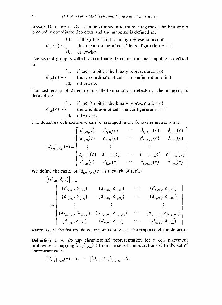
answer. Detectors in DB, a can be grouped into three categories. The first group is called x-coordinate detectors and the mapping is defined as:

1, if the j th bit in the binary representat ion of

di,,~(c) = the x coordinate of cell i in configuration c is 1

0, otherwise.

The second group is called y-coordinate detectors and the mapping is defined as:


di,y,(c ) = the y coordinate of cell i in configuration c is 1

0, otherwise.

The last group of detectors is called orientation detectors. The mapping is defined as:


d~,o~(C) = the orientation of cell i in configuration c is 1

0, otherwise.

The detectors defined above can be arranged in the following matrix form:

di,m,(c ) di,.,2(c ) "'" di~.,,, ' ,(c) di,,nm(c )

di2m,(c) di2,,2(c) "'" di2,,m_,(C ) di>n~(c) =

d, , , ,n ,(c) di,_~,n2(c ) "'"

d,,.,,(c) di,,n2(c ) " '"

We define the range of [di..]l×,.(c) as a matrix of tuples

[ ( ¢ , , , 6i,,)],xm

(di,..,,6i,,n,) ( d , , . . 2 , . . .

(did.n,, '5i2,.,) ( di2,.~, 6,2,.~) " .

d,,,,nm_,(c) di, lmm(C) di,,nm_,(C) di,mm(c)

(dil,~m, ~ia,-o. ,)

(di2,n,., ~i2,n,.)

(dil-l,~l' ~il I,~l) (di/-l,'02' all 1,'02) "'" (dil l,~rn' all 1, ~m)

(di,,n,, ¢~i,,r),) (dit,~o 2, ¢~il,rl2) " '" (dit,.m, ~it,~l.)

where di, n is the feature detector name and 6i. n is the response of the detector.

Definition 1. A bit-map chromosomal representat ion for a cell placement problem is a mapping [di,n]l×m(C) from the set of configurations C to the set of chromosomes S.

[di , . l ,×m(c ) • C ~ [(di, ", a i . . ) ] ,×m=S ,

H. Chan et al. / Module placement by genetic adaptiee search 57

where [di,n]txm(C) is a matrix of detectors formed by the elements in the set

DI, a and di,n(¢)= ~i,n E {0, 1}.

Observation 2. A cell configuration c ~ C represented by a bit-map chromosome s ~ S is invariant under arbitrary numbers of row and column interchanges of s.

This follows from the fact that the detector and response are coupled together as an ordered pair. If a pair is moved to a different row or column, the same detector will still have the same response. In other words, row and column interchanges change the coding of the configuration as a chromosome, but do not change the cell placement. Example 1. Suppose there are four cells (L = 4) to be placed on a chip of grid size 8 x 8 (i.e., n x = ny = 3) in eight possible orientations (n o = 3). This implies that m = 9. Let the four cells be as shown in Fig. 2(a). Figure 2(b) shows a particular bit-map chromosome representat ion and its corresponding placement configuration.

The physical analogy to genetics is made when we note that each feature (di,n, t~i, n) in a placement configuration is a gene in the chromosome, and they are arranged physically in the form of an array [(di, n, •i,n)]lxm. Each gene in a chromosome thus carries a particular feature that exists in the corresponding configuration. The alphabet of the gene used here is binary and, therefore, it satisfies one of the criteria for efficient search as we listed above. The details of the algorithm are shown in Fig. 3.

3.3. Bit-map crossover operator

Crossover is the primary genetic operator for reproduction. It produces new configurations, called offspring, by randomly combining the current configurations, called the parents. During the process of crossover, genes that carry good placement propert ies from both parents will have a chance to combine forming bet ter solutions. Hence, this operat ion will cause the quality of solutions in a population to improve. However, the design of the chromosomal representat ion and the genetic operator must ensure that the chromosome produced after a crossover operat ion does not contain any identical genes (i.e., a cell does not duplicate due to random cut and paste). Any postprocessing to eliminate duplication of genes will cause a degradation in search efficiency [13] and is undesirable. In this paper, a new genetic crossover operator is introduced. Each chromosome it produces corresponds to a legal p lacement solution and, therefore, our operator is conflict-free, and satisfies the second criterion for efficient search listed in Section 2.

The crossover operation consists of two parts. Let two chromosomes which combine to form an offspring be A and B (the parents). It may be noted that due to previous crossover and other transformations, the positions of the detectors in A may not be the same as in B. A homologous reordering

58 H. Chan et al. / Module placement by genetic adaptiue search

Cell 1 Cel l 2 Cell 3 Cell 4

(a)

(d1,.2, O) (d1,~1, O)

(d2,.2, i) (d2,.1, 1)

(d3.~2, 1) (d3,~,, 0)

(d4,x2, t) (d4,xl, 1)

(d,,.o, 1) (d,,~2, O) (d,,u,, 1) (d,,vo, 1) (dx,o2, 1)

(d2,.o, O) (d2,~2, O) (d~,~,, 1) (d2,uo, O) (d2.o2, O)

(d~,~o, O) (d3.u2, 1) (d3,~, 1) (d3,~o, O) (d3,o2, O)

(d4.~o, O) (d4,~2, 1) (d4,~,, 1) (d4,~o, O) (d4,o2, O)

(dl,ol, 0) (dl,oO, 0)

(d2,o,, O) (d2,oo, 1)

(d~,o,, 0) (d~,oo, 1)

(d~,o,, o) (d~,oo, ~)

I • • - - r - - - r - - -

Fig. 2. (a) Input cells; (b) a bitmap representation and its corresponding cell configuration.

operation [13] is, therefore, applied first to chromosome B. The effect of this operation is to alter the position of its detectors such that both A and B are homologous, or have the same arrangement of detectors. The operation consists of a number of pairwise row and column interchanges. Observation 2 points out that this operation will not change the physical configuration and, therefore, it will not affect the efficiency of the search. Since the reordering operation requires sorting, it is easy to see that the time complexity with a bit-map representation is g(L + m), where g(x) is the time for sorting x elements. This time complexity is much smaller than g(L × m) which is required if a bit-string representation is used. After the reordering operation is performed to rearrange the detectors, two points, say l* and m*, are picked randomly with uniform probability between 1 and l - 1, and 1 and m - 1, respectively. A vertical and a horizontal line are drawn on the bit-map of A and B along row l* and column m* respectively. Both A and B are then divided into four sub-bitmaps by these lines. The intersection of these lines is called a crosspoint (l*, m*). The offspring is formed by combining the upper-left and lower-right sub-bitmaps from A, and the lower-right and upper-left sub-bitmaps from B. The detailed procedure for crossover is given below. An example is shown in Fig. 4. Figure 5

H. Chan et aL / Module placement by genetic adaptive search 59

P R O C E D U R E GAMP beg in

Input cell geometry and net-list; Initialize population by randomly generating

M solutions P(0) = {Sl(0), S~(0), . . . , SM-I(O), SM(0)} ; Evaluate the fitness F(O) = {fl(O), f~(O),-.., fM-l(O), fM(O)} ; Calculate the average fitness of population P(O)

.fp(0) = EM=IA(O)/M ; for i = 0 to G {Number of generation.} beg in

for j = 0 to O {No of offspring.} beg in

Define a random variable Rand on [ = {1,2, 3- . . , M} by assigning each m E I n probability f,n(i)/fp(i) , draw a number Rand(j) E I from Rand ;

Define a random variable Unif on I = {1, 2, 3 . . . , M} by assigning each m E I an equal probability 1/M. Draw a number Unif(j) from Uuif;

Apply crossover with probability Pc to parents Sran~(i)(i) , Sunq(D(i) from population P(i) ;

Select one of the offspring equilikely, and let it be Sc ; Apply inversion with probability Pt to Sc to form Se~ ; Apply mutation with probability PM to Sel to form Sj(i) ; Add the offspring Sj(i) in

P' = {S'~(i), S'~(i),..., ~(i)}; end ;

Evaluate the fitness {ls;,fs•,'" ",fs o } of P ' ;

Find the first M best solutions from the set P(i) U P', assign them to the next generation P(i + 1) and update current fitness F(i+ l) ;

Calculate the average performance of population P(i + 17 , L,:,(i + 1) = EM=ofk(i+ 1)/M ;

end; Output the best solution from population P(G) ;

end;

Fig. 3. G e n e t i c a l g o r i t h m for cell p l a c e m e n t s .

shows the configurations of the offspring when the crossover operation is performed on two parents. It is worthwhile to point out that the configurations of the parents do not change before and after the reordering operation, as described in Observation 2. Figure 5 also shows the process of feature passing between generations. Here, the location and the orientation of cell 1 in offspring 1 is the result of combining the location feature from cell 1 in parentl and the orientation feature from cell 1 in parent 2. Similar feature combination occurred for cell 2. Furthermore, the x-coordinate of cell 4 in parent~ is combined with the y-coordinate of cell 4 in parent 2 to form the new location of cell 4 in offspring 1. This example shows the usefulness of passing features by crossover which constitutes the primary difference between our genetic approach and the other search techniques.

Procedure CROSSOVER(A, B) Step 1: Reorder B to make it homologous to A.

I (dl ,

x20

(dl,x

lO)

(dl.x

O 1 )

(d

l.y20

) (d

l,yl 1

) (d

l,yO

l )

(d2,

x21)

(d

2.xl

1 )

(d2.x

o 0 )

(d2,

y20)

(d

2.yl

1)

(d2,~

o 0 )

(d3,

x21)

(d

3.xl

ll)

(d3,

x(lO

) (d

3,,2

1)

(d3,

, 11 )

(d3.

, 00 )

(d

4.,2

1 )

(d4,

xl l )

(d

<xo 0

) (d

4.y21

) (d

4,yl

l )

(d4,

, 00 )

t

(.,,0

2')

(<.o,

O) (<

.,,oO)

][(<..

o,)

(a~,

o2o)

(d

2,o,

O) (

.2.,,

ol)|[

(.,..o

O)

(.~,,.

2o)

(~.,,

o)

(.~.o

,,1)||

(<,.,

,o)

(<,o~

O)

(<,,,

,o)

(d~.

ool)J

k(d~

,.ol)

[ (a

l,~20

) (d

l,.l O

) (d

l,xo 1

) (d

l,?2 O

) (d

l,yll)

I (

dl,,

01)

(dl,o

21 )

(dl.o

lO)

(d2,

~21)

(d

2,xl

1)

(d2.

*()O

) (d

2,y2

0 )

(d2,

yll)

] (d

2,,O

O)

(d2.o

2 O)

(d2,o

lO)

(d3,x

21

(d3.x

lO)

(d3.

xO O)

(d

3,,2

1)

("3,

"11)

/ ("

3000

) (d

3,o2

0)

(d3,o

lO)

[(d4

,x21

) (d

4.xl

l) (d

4.,o

O)

(da,z

. 21 )

(d

4,,,l

)/ (d

<,,00

) (&

o20)

(a

a,o,

o)

i (dl,a

20 )

(al.x

,o)

(.1,xO

1 )

(dl,y

20 )

("l,y

l 1 )

(dl,,

(.1)

("1.o2

0 )

(d2,

x21 )

(d

2,xt

1)

(d2,

xo 0 )

(d

2.> 20

) (d

2,>')1

) (d

2,>,o 0

) (d

2 ,,2

1)

(d3,x

21 )

(d3,x

10)

(d3.x

{) ())

(d

3,y2

1)

(d3,

y,l)

(d3,

yo 1 )

(d

3.o2

0)

(<.~

2o)

(.4.~

o)

(d~,

~,,l)

(d~

,.20

(<.,.

,0

(d4.

,oO

) (<

.o2o

)

(da,

, 01 )

(d

4,xl

1 )

(d4,

,20 )

(d

4,yl

1 )

(d4,

olO

) (d

4,, 2

1 )

(d4,o

20 )

(d4,

oO 1 )

(d

3,, o

l )

(d3.

xll)

(d3,x

20 )

(a3.,

,11 )

(a3,

ol 0 )

(d

3,, 2

0)

("3,

020 )

(d

3,o[

) 0 )

(dl.,

ol)

(dl,,

i l )

(dl.,

21)

(dlo

10)

(d

l,otO

) (d

l,, 2

0 )

(dl,o

2 O)

(dl,o

oO)

("2.

, 00 )

(d

2,xl

O)

(d2,

x21 )

(d

e.,,

0 )

(d2.o

l l )

(d2.

)21

) ("2

,o21

) (d

2,oo

1 )

I Ho

mol

ogou

s

(dl,o

OO

) 7 [

(dl

.x21

)

(<o,

,,)||

(<~2

~)

(",,,,

o')| /

('3.~2

°) (d

<o,)l

)J k

(d<~

2 °)

L ("

,.~,0

(<

.x00

) (.

.....

) (.,

.,,0)

(d

2.xl

0 )

(d2.

rlI1

) (d

2., 2

1 )

(d2.

, I 0 )

(d

3,xl

1 )

(d3,

xoO

) (d

3.~. 20

) (d

3.:. I

1 )

(d4,

xl 1

) (d

4,x(, 1

) (d

4.v21

) (d

4., 1

1)

(dL

yl,1

) (d

l,o20

) (d

l.olO

) (d

,,o(,O

) (d

2,, 0

0)

(d2,

o21 )

(d

2,o,

1 )

(d2.

oO l )

(d

34

1)

(d3.

o20)

(d

3,olO

) (d

3,o,,O

)

(d4.

;o 1 )

(d

4,o2

0)

(d4.o

,O)

(da,

o(,1

)

(.,.,,

o)

(<o0

0>][(

<x~,>

(<

x,l)

(<.9

>

(<,~0

) (.,

.,0)

(a2.o

,1)

(~2.

o,,1

)|[(~

2,~1

) (<

,~10

) (,2

x01)

("

2,,2

0 (<

,,°)

(d<.

,0)

(d<<

,,,1)

Jk(d

4~20

(d

~.l)

(<

,.~,0

) (d

~.,.

0 (d

4,,l

1 )

.

(d,,y

01)

(dl.o

21)

(dl,o

l0)

(dl,o

00)

(d2.

,,,0)

(d

2,,,2

0) (

d2,,,

,O)

(a~,

o,,1

) (d

3,yoO

) (d

3,o2

0)

(d3,

ol O

) (d

3,,,o

1 )

(d4,

,.ol)

(d4.

o20)

(d

4.olO

) (d

4,,,o

1 )

Fig.

4.

An

exam

ple

to s

how

the

cro

ssov

er o

pera

tion

.

.:a:

e~

~a g::a,.,

=2

e~ =a.

g


~ " ' ' , ' t

. ° . , . . . ° . . . , . . . ,V---1

parent

i [ ~ i . . . . . "4

* "IF--" ~

. . . . . I - 1 - D - .

D ..... p.. parent 2

Homologous

-- - - I - 1 - D - -

31 " " "n Offspring Offspring 2

Fig. 5. An example to show how the crossover operation in Fig. 4 reproduces offspring.

Step 2: Randomly pick two points l* and m* between 1 and l - 1" and 1 and m - 1, respectively.

Step 3: Split A and B into four sub-bit-maps at crosspoint (l*, m*).

Step 4: Produce two offspring.

END

Boo B01 ]

IAoo Boll [~oo Ao,] 01 = [-Bl~llV-z41?j, 02 = [Alo-~- /~ l? j

62 H. Chan et a L / Module placement by genetic adaptive search

3.4. Bitmap inversion operator

If only crossover is used, a gene will be inherited by the offspring with a probability that depends on where the gene is placed in a chromosome and which genes are in its neighbourhood. Holland [13] showed that the inversion operator is useful for dealing with this clustering effect among genes in a chromosome. Inversion shuffles the arrangement of genes in a chromosome by exchanging its rows and columns randomly. It weakens the linkage among genes in a chromosome which permits more uniform propagation of features from parents to offspring during reproduction. After inversion is applied, each gene will have an equal opportunity to be inherited by the offspring, less dependent on where the gene is placed and which gene is in its neighborhood. Informally, it prevents a bad gene from continuously tagging along with a good gene, which happens to be next to it in the matrix. By shuffling the entries in the matrix, inversion allows various combinations of genes to be passed from the parents to the offspring. A detailed procedure for inversion is given below.

Procedure INVERSION(,4) Step 1: Randomly pick two points l~ and l~' between 1 and l - 1. Step 2: Let a i be the ith row of `4, then ,4 can be split into three parts

,4 = [a l , az,... ,al?, al?+l,...,at~, at~+l , . . . ,a l ] T. Step 3: Perform column inversion, B = ta 1, a2,...,al~,, az~, atf_ 1 . . . . , az?+~,

al~ + l, . . . , a l ] y Step 4: Randomly pick two points m~ and m~ between 1 and m - 1. Step 5: Let b i be the ith column of B, then B can be split into three parts

B = [ b l , bz , . . . ,bm~( , b r n , + l , . . . , b m , , bm~J+l,.. . ,bm]. Step 6: Perform row inversion. C' = [b~, b 2 . . . . , bm~(, bm~, b m , _ l , . . . , bm~+l,

bm~+l , . . . , bm]. Step 7: Output C.

END Procedure

3.5. Bit-map mutation operator

Mutation serves as a background operator that supplies new genetic material during reproduction by randomly changing genes in a chromosome at a rate pre-defined by the algorithm. Since the number of chromosomes represented in a population is finite, it is possible that a particular feature detector, say d~j, responds to zero (or one) for all the chromosomes presented in a population. If this happens, the gene is said to be lost from a population. Both crossover and inversion cannot recover it. In other words, crossover and inversion cannot generate all possible placement solutions for trial. The algorithm will be trapped in local maximum if only crossover and inversion are used. Mutation, therefore, provides a way to widen the range of genes in a population to ensure that no gene permanently disappears from the population. However, the random flip- ping of the genes causes loss of information acquired from the previous

H. Chan et aL / Module placement by genetic adaptive search 63

generations and, therefore, it distracts the algorithm from finding the optimal solution. Hence, the mutation rate is kept very low in practice. The mutation operation is described as follows:

Procedure MUTA TIO N(A) for each gene in A.

Step 1: Pick a point p uniformly between 0 and 1. Step 2: If p ~< PM, the mutation rate, then invert the bit value of the gene.

END Procedure

4. Theoretical aspects of GAMP

In order to direct the search towards the goal, an efficient algorithm should identify features in an intermediate solution that contribute to its goodness, and this knowledge should be exploited properly to guide the search. Although the basic procedure of the genetic algorithm is very simple, it has been shown that it does have this learning capability [13,23]. In brief, the genetic algorithm divides the search space into schemata having some common features. During each generation, it estimates the average fitness of the various classes, and favors the selection of members from the classes having higher fitness values. The current estimated fitness of the classes thus provides a basis for controlling the search direction at each generation.

First, we see how the classes are formed by identifying the common features. Since genes in a chromosome determine a set of features that are related to the locations in a configuration, it is easy to see that each gene imposes a restriction on the region where a cell can be placed. For each gene (d~.j, 6), we define the constraint region A(a~) for cell i in configuration c as the entire region, where the detector dij(c) gives the value ~ whenever cell i is placed inside the region. Hence, the definition of the y e s / n o detector mapping can be restated recur- sively, in terms of constraint regions, as follows:

1, cell i located inside constraint region A(al,j,1)

di,j(c) = 0, cell i located inside constraint region A(d,.,o ).

In order to decompose the search space C into subsets, where each configuration in a subset shares common features, let the symbol [] be a don't care symbol. Then (di,j, []) indicates that we "don' t care" what value occurs at the output of the detector, di, i. Thus [(d~,,~, 1)(d1,,2, 1)(d~,~, []) . . . (dl . ,m, ~3)] designates a subset of all configurations in C having cell 1 placed inside the intersection of constraint regions A(a ' 1) and A, a 1,. The set of all schemata involving the combination of [], 0, an'~'l form tl~e~']~roduct set £ --- [(di, j, Aij)], which is a matrix with elements being tuples containing detector names, and Aij ~ {0, 1, []}. We formalize the idea as follows:

64 H. Chan eta[. / Module placement by genetic adaptive search

Definition 2. A schema ~ in a bi tmap chromosome representat ion, is an l x m matrix [(di, n, A~,n)]l× m where each e lement in the matrix is a tuple. The first e lement in the tuple is a detector 's name d~,n ~ Dt, a while the second e lement is a symbol Ai, ~ ~ {0, 1, D}.

The relationship of chromosomes in S can be defined as follows:

Definition 3. Two chromosomes A and B in a bi tmap chromosomal representation are said to be e lements of schema s c =[(di , ", Ai,n)]lx m, if for all i ~ l, r / ~ A, 1. Whenever (di,~, Ai, j) = (di,j, D)

di,i(A), d i j (B) can be of any value. 2. Whenever (dij , Aij) 4: (di,j, D)

di j (A) = di,j(B) = Ai, j. We denote this relation by saying that A, B ~ ~.

A schema, therefore, corresponds to the set of solutions that are selected from its resultant constraint regions, which are obta ined by the intersection of the constraint regions defined by each individual element.

The following example illustrates the concept of a schema. Let the schema, of four arbitrary cells be given by Fig. 6(a). For this example, let the x and y coordinates consist of three bits, n s = ny = 3 and n o = 0. The first row of ~ has all six detectors defined, and it gives the x, y coordinates for cell 1 as (2, 5). This is shown by the single shaded square in Fig. 6(b). The o ther rows of ~: contain don ' t cares. For example, the second row specifies only that the high order bit of y = 1. This is shown by the large shaded region for cell 2 in Fig. 6(b). The constraint regions for cells 3 and 4 are also shown. The various configurations constructed by cells being picked up from the corresponding shaded regions belong to the same class. Thus for this example, there are al together 1 x 32 x 16 x 16 = 8192 different configurations in this schema, since cells 1 - . - 4 can occupy respectively 1, 32, 16, and 16 possible locations, as indicated by the size of the shaded regions.

In order to search efficiently, the genetic algori thm divides the search space into many schemata having some impor tant common features, and it adaptively selects solutions from these schemata by estimating the fitness or quality of the classes. Since equivalence classes are constraint regions in our p lacement problem, the genetic algori thm generates more solutions with cells coming from constraint regions that have higher es t imated average performance. The following theorem illustrates this idea.

Theorem 1. By using bitmap crossouer operator in the genetic algorithm, the expected proportion of an l x m schema ~ represented in the population at time t + l is

^

M~(t + 1) = (1 - Z(~)Pc) (a - PM) °¢~)f~(t) f ( t ) Me(t) .


= (d~.:,aO) (d~.=-,O) (d,.=30) (d~.uxl) (d~.,~Cl) (d~.,on)

(d~,=xl) (dz,=~O) (dz,xsO) (dz,,, n) (d~,,~l) (dz,~oO)

(d,,~l 0 ) (d,,x20) (d,,,3 n ) (d,,~l 0 ) (d,,u21) (d,,l~3 r'l )

(a)

A y A Y

I I |@i!iii:::¥ii::lii::iii!l #li::::ii:,ii~l:j~!|

" " " ' 1 1 1 I I I I I I I I I x I l i l l i l l x I I .... I~- I I I I I I I I ....

C e l l 1 C e l l 2

AY ~. Y

I[ ~l~l~i~!H l~i~li~i~| ~I~ II I I I I I I I I I I I I I I l i l I I l l i l I I I

i l l i I I I l l x I I I i l l l J x I I I I I I I....D.,. I I I I I I I I .... I ~ -

Cell 3 Cell 4

(b)

Fig. 6. (a) An equivalent class ~; (b) the constraint regions whichconta in a solution set of 8192 different configurations.

where Me(t) is the expected number of solutions in the current population that belong to ~; re(t) is the estimated fitness of ~; f ( t ) is the estimated average fitness of the population at time t; Z(~) is the linkage among genes which is class dependent; Pc is the crossover rate; P~4 is the mutation rate; o( ~ ) is the number of non- [] elements in ~.

P r o o f . Let A be a chromosome in the current population. Since parents selected for reproduction are based on the fitness of chromosomes, the expected number of chromosomes produced from A in one generation is PcfA/ f ( t ) , where fA is the fitness of A. Therefore, the expected number of offspring produced from a schema s c in one generation using only crossover is

eeL, ec (t) E - M e ( t ) - -

A e~,Aee(t) f ( t ) f ( t )

where Me(t) is the expected number of chromosomes belonging to ~ at time t.


^

It is worthwhile to notice that f~(t) is an estimate of the average fitness of s c based on finite observations of solutions existing in the current population. Supposing A ~ : , it is easy to see that the offspring from A might not necessarily belong to ~:. Let this possibility be Z(~C), and is determined by the relative arrangement among elements in the schema s c. If mutation is applied, the expected number of solutions which do not belong to s c in the next generation will be

^

eo/ ( t ) M¢,) f ( t ) Z(sC)(1-

Therefore, the expected number of chromosomes that belong to s c in the next generation is

^

q.e.d.

Remark 1. Since inversion randomly alters the relative positions of genes by exchanging rows and columns, the term Z(s c) tends to be constant as inversion is applied. Thus, Theorem 1 provides a direct relation between the number of chromosomes belonging to a particular class at two consecutive generations. That is, if the current estimated average fitness of a schema s c is above (below) average, the number of solutions taken from s c will increase (decrease) in the next generation. Hence, the genetic algorithm has the ability to bias the future construction of solutions using the past observed information.

Remark 2. The estimated fitness ~ ( t ) is based on a finite number of observations of solutions that belong to s c at time t. For each fitness evaluation of a chromosome, it is found that a number of aM 3 classes will be estimated simultaneously [25], where a is a constant and M is the population size. The estimated fitness f¢(t) of a large number of classes will, therefore, be refined in each generation.

Remark 3. Assuming that the term Z(~:) is constant and PM is small, and also assuming that the fraction of the estimated performance of ¢ to the overall performance is constant and is equal to k for t generations, then, we have

M (t + =

Hence, the genetic algorithm will exponentially increase the number of solutions that belong to the class s c in the population if the factor k is greater than one. Therefore, it has the ability to explore the promising parts of the solution space more deeply.

H. Chan et al. / Module placernent by genetic adaptive search 67

5. Simulation results

The genetic algorithm was used for macro cell placement for five M C N C benchmark circuits. Experiments indicate that our algorithm converges rapidly during the early phase of the run. All computat ions were carried out on a SUN Sparkstation 1 + desktop workstation. The program was writ ten in C, using 2000 lines of code.

In our algorithm, the populat ion in the next generation is obtained by keeping the best configurations among the parents and their offspring. An alternative way is to select configurations probabilistically based on their fitness. That is, the configuration with higher fitness has a greater chance of being selected for the next generation. However, experiments showed that our replacement strategy obtained a bet ter result. In our selection strategy for crossover, the first parent is selected based on its fitness, while the second parent is a random trial from the population. Experiments show that the algorithm converges to local minimum if both parent are selected among good configurations. This is because good parents have too many features in common and their offspring will not have enough diversity in their genes.

Experiments were run to determine the appropriate values of crossover, inversion and mutat ion probabilities. These experiments were run on the 33 cell M C N C benchmark circuit ami33. The performance measure was the final fitness obtained after a fixed number of generations. The number of generations (1500 for this circuit) was chosen such that there is little or no further improvement if the algorithm is run for a longer time. Table 1 shows the result of varying the mutat ion rate. Low mutat ion rates such as 0.001 or 0.005 give the best performance. Table 2 shows the result of different inversion rates and Table 3 shows

Table 1 Effect of mutation rate on fitness

Mutation rate Fitness Wire length

0.005 0.141 35490 0.001 0.179 27728 0.002 0.155 32237 0.003 0.143 34691 0.004 0.162 29366 0.005 0.168 29565 0.006 0.147 34057 0.007 0.161 30862 0.008 0.146 33718 0.009 0.156 31114 0.01 0.137 36481 0.015 0.137 34052 0.02 0.123 36993 0.03 0.115 32485 0.04 0.106 36984 0.05 0.105 29857


Table 2 Effect of inversion rate on fitness

Inversion rate Fitness Wire length

0.05 0.143 32637 0.1 0.152 32271 0.15 0.145 33331 0.2 0.146 33208 0.25 0.169 29081 0.3 0.162 30862 0.4 0.145 337.18 0.5 0.157 30555

the effect of crossover rate. The relationship between the inversion rate and the final fitness is a little less pronounced, and the effect of varying the crossover rate appears to be almost random. For further experiments, we picked the best values of the parameters as follows.

Crossover rate: 0.8, inversion rate: 0.25, mutation rate: 0.01. Note from the results that the final wire length is not a good measure of the

performance of the genetic algorithm. For a given fitness, it is possible to get different wire lengths, since the fitness also depends on the chip bounding area. If the genetic algorithm is optimized to obtain the best possible final fitness, then adjusting the relative weights for wire length, bounding area penalties provides a good compromise between wire length and area.

Figure 7 shows plots of the data in Tables 1-3. Figure 8 shows the effect of the mutation rate on the fitness throughout the run, and Fig. 9 shows similar results for the inversion rate.

With these values of the parameters, more experiments were run on the 5 MCNC benchmark circuits (Table 4) to determine the final wire length and chip area of the routed chip. The cells were placed using GAMP. The routing and compaction was done using the Mosaico CAD system. Table 4 gives the results. Figure 10 shows the wire length, chip bounding area, cell overlap area, and outside area for the 33 cell ami33 circuit. The outside area is the area of the

Table 3 Effect of crossover rate on fitness

Crossover rate Fitness Wire length

0.99 0.179 28001 0.95 0.138 35670 0.9 0.179 27816 0.8 0.197 25312 0.7 0.160 31104 0.6 0.161 30798 0.5 0.160 30144 0.4 0.174 27501

H. Chan et al. / Module placement by genetic adaptiue search 69

cells lying outside the given boundary, and like overlap area should be reduced to zero. The bounding area is the minimal bounding area of the cells at any time. Figure 11 shows the fitness. This increases monotonically, since a good solution is never rejected in favor of an inferior one.

The evaluation of fitness takes most of the computation time for our algorithm, about 95% of the total processing time. The run time efficiency of our algorithm, therefore, depends on how efficiently the cost evaluation is done. In our implementation, the wire length is estimated by the half-perimeter of the smallest rectangle enclosing the pins of the net. The computation of the exact overlapping area of the cells is very costly. We estimated it by dividing the chip

0

0

0

0

~ o

-~ 0 14

0 13

0 12

0 11

0 .1

19

18

17

16

15

0.17

0.165

0.16

.~ 0 .155 U..,

0.15

0.145

& (a)

i i i i i i i i i i

0 • Ol 0 • 02 0 • 03 0 • 04 0 • 05

(a) Performance for various Mutation rates

, , , , , ,

0.14 ~ , , , , ~

0 . 0 5 0 .1 0 .15 0 .2 0 .25 0 .3 0 .35 0 .4

(b) Performance for various Inversion rates Fig. 7. Effect of genetic parameters on fitness.

i

0.45 0.5


0.2

0.19

0.18

~ 0 . 1 7

B 0 . 1 6

0 . 1 5

0 . 1 4

0 . 1 3 0 . 4

i i i i 01.9 o . ~ 0 . 6 o . v 0 . 8

(c) Performance for various Crossover rates

Fig. 7. (continued).

into a 256 X 256 grid. All the grid squares covered by each macro cell are scanned. The first time a square is visited, it is marked as occupied. Each successive time the same square is visited, it is counted as an overlap. The total overlap area is equal to the overlap square count times the area of each square. This overlap determination algorithm has a complexity O(AT), where A T is the

0.18 , i , , i i ,

0.16

,M=O. 001 , - -

, M=O. 004 ....

,M=O.O09 , -..

'M=O .01' ......

'M~O .02' ----

'M~O.03' - " "

0.14 ---- --~-'----~ a 2

s r -- , ....... ; ...... •.

p- • ......... , ............... rr

......... J o.12 /...,:...- .... rj .............

U r~ r-J t j+...: I - J

........ f' [._a ....... o. 1 f I-Lr' -- =. ..............

•-J2-'_

0.08

0.06

0.04 I I I I I I I

200 400 600 800 1000 1200 1400

Fig. 8, Effect of mutation rate on fitness.

1600


0.18

0.16

0.14

0.12

0.I

0.08

0.06

,i=0.05 , - -

J- ' I=0. i' ---"

.~.w -~ ' I=0.15 ' j,-° I _.r t - - ~ - rl'~'O-7"?" ......

-- - - ~ - - ' I=O. 2~'..--- "- .~'~~' _.- r'~--- .-'Y=O'. 5 ....

r .... .:.'_ .... __. _--~-~. _ I

.J 8 --',"

/Y 0 . 0 4 I I I I I I I

0 200 400 600 800 i000 1200 1400

Fig. 9. Effect of inversion rate on fitness.

1600

Table 4 Performance statistics of GAMP for five MCNC Benchmark circuits

Circuit Cells Nets Final wire Final chip length area

apte 9 97 590.6K 61.8M xerox 10 203 1038K 32.6M hp 11 83 365K 42.9M ami33 33 123 278.5K 1.23M ami49 49 408 2077K * -

* Bounding rectangle wire length

Table 5 CPU time usage of GAMP

Circuit Total Evaluation Crossover Mutation Inversion CPU sec. % % % %

apte 1692 97 0.8 0.6 0.04 xerox 4099 98 0.6 0.5 0.03 hp 2408 97 1.0 0.8 0.05 ami33 6692 95 1.8 1.7 0.06 ami49 21552 95 1.6 1.5 0.05

7 2 H. Chan et al. / Module placement by genetic adaptive search

&

m

1 6 0 . 0 0 - -

1 4 0 . 0 0 - - -

1 2 0 . 0 0 - -

100.00 - -

80.00 - - -

: ~ ~ = ~ _ _ _ Bounding. Area . . . . ~

, i I ~ _ _ - J

:l ;i ',1 i i " ii

i i :!

Wire length

', , - " - ". ;'",._, Outside Area

lap area

0 . 0 0

55.00 ]

50.00

45.00 _

40.00

35.00 ~ L ~

30.00. l

25.00. _ _

20.00.

15.00.

0.130

100.00 2 0 0 . 0 0 3 0 0 . 0 0

G e n e r a t i o n s

Fig. 10. Optimization curve of GAMP.

I r J

100.00 200.00 300.00 Generat ions

Fig. 11. Optimization curve of GAMP.

4 0 0 . 0 0

400.00

H. Chan et al. / Module placement by genetic adaptiue search 73

total area of the macro cells (not the chip area available). Experiments showed that the resolution of grid we used is fine enough for accurate overlapping area estimation.

Table 5 shows the run time and its division among the genetic operators. Due to the use of 2-dimensional bit-map chromosomes, the crossover, inversion and mutat ion operators are very fast, and take a negligible amount of time compared to the evaluation. This disproves the usual argument that genetic operators are complex and CPU-intensive.

Fig. 12. Placement result for the "xerox" netlist.

7 4 14, Chan et al. / Module placement by genetic adaptive search

it

:il

: :

! i

i

I!. ii

l i i i i l i i l i

r _

T~

!

! :

Fig. 13. Placement result for the "apte" netlist.

= / i

Figures 12 and 13 show the placement results of two MCNC benchmarks. Figure 14 shows the evolution of the placement as the algorithm proceeds.

6. Conclusions

This paper presents new insights into the application of the genetic algorithm in block and module placement. A new bit-map chromosome representation and a set of genetic operators for the placement problem are presented. This chromosome representation divides the entire search space into a large set of

1t. Chan et aL / Module placement by genetic adaptive search 75

o

(el

- r: l

n (b) (g)

I'h ~ (h)

o ,(c) ~oo ot~ (,)

o ~n(~ (d) Fig. 14. Evolution of circuit 1 from (a) initial placement to (j) final placement.

feature-equivalent classes or schemata where each class designates a set of solutions with cells selected from the designated regions. The genetic algorithm adaptively biases the search based on the current estimated performance of schemata that exist in a finite population. By arranging genes in a two-dimensional fashion, the bit-map chromosome reduces the amount of time used by the genetic algorithm, as compared to the bit-string representation. Future work will focus on the integration of floorplanning, standard cell and macro block placement using the bit-map representation.

Our implementation suffered from non-linear interactions between the genes, and the resultant degrading of search efficiency, and we need to find a better genetic coding for the placement problem.

We conclude that the genetic algorithm is a promising searching method for the cell placement problem that warrants further investigation.

Acknowledgements

This research was partially supported by the ONR grant number 00014-85-K- 0122, Digital Equipment Corp faculty development grant, University of Michi- gan faculty grant, and the Research Initiation Program of the National Science Foundation under the grant number MIP-8808978.

76

References

H. Chan et al. / Module placement by genetic adaptive search

[1] N.R. Quinn and M.A. Breuer, A forced directed component placement procedure for printed circuit boards, IEEE Trans. Circuits and Systems CAS-26 (6) (June 1979).

[2] M. Hanan, P.K. Wollf and B.J. Agule, Some experimental results on placement techniques. Proc. 13th Design Automation Conf. (1976) 214-224.

[3] Ulrich Lauther, A min-cut placement algorithm for general cell assemblies based on a graph representation, Proc. 16th Design Automation Conf. (1979) 1-10.

[4] L.I. Corrigan, A placement capability based on partitioning, Proc. 16th Design Automation Conf. (1979) 406-413.

[5] C. Sechen, D. Braun and A. Sangiovanni-Vincentelli, ThunderBird: A complete standard cells layout package, IEEE J. Solid-State Circuits 23 (2) (April 1988).

[6] C. Sechen and A. Sangiovanni-Vincentelli, TimberWolf 3.2: A new standard cell placement and global routing package, Proc. 23rd A C M / IEEE Design Automation Conf. (1986) 432-439.

[7] S. Kirkpatrick, C.D. Gelatt and M.P. Vecchi, Optimization by simulated annealing, Science 220 (4598) (13 May, 1983) 671-680.

[8] C. Cheng and E. Kuh, Module placement based on resistive network optimization, IEEE Trans. Computer-Aided Design CAD-3 (July 1984) 218-225.

[9] A. Casotto, F. Romeo and A. Sangiovanni-Vincentelli, A parallel simulated annealing algorithm for the placement of Macro cells, IEEE Trans. Computer-Aided Design CAD-6 (5) (Sept. 1987).

[10] M.D. Durand, Accuracy vs. speed in placement, IEEE Design and Test of Computers (June 1989) 8-34.

[11] J.P. Cohoon and W.D. Paris, Genetic placement, Proc. IEEE Int. Conf. Computer-Aided Design, 1986.

[12] K. Shahookar and P. Mazumder, A genetic approach to standard cell placement using meta-genetic parameter optimization, IEEE Trans. Computer-Aided Design 9 (5) (May 1990) 500-511.

[13] J.H. Holland, Adaptation in Natural and Artificial Systems. (The University of Michigan Press, Ann Arbor, 1975).

[14] K.A. De Jong, An analysis of the behavior of a class of genetic adaptive systems, Doctoral Dissertation, University of Michigan, Dissertation Abstracts International 36(10), 5140B (University of Microfilms No. 76-9381), 1975.

[15] R.A. Fisher, The genetic theory of natural selection (Dover, New York, 1958). [16] J.R. Sampson, Biological Information Processing (Wiley, New York, 1984). [17] N.A. Barricelli, Symbiogenetic evolution processes realized by artificial methods, Methods 9

(35-36) (1957) 143-182. [18] A.S. Fraser, Simulation of genetic system by automatic digital computers. 5-linkage, domi-

nance and epistasis, Biometrical Genetics (1960) 70-83. [19] F.G. Martin and C.C. Cockerham, High-Speed selection studies, Biometrical Genetics (1960)

35-45. [20] J.D. Bagley, The behavior of adaptive systems which employ genetic and correlation algo-

rithms, Doctoral Dissertation, University of Michigan, Ann Arbor, 1967. [21] A.L. Samuel, Some studies in machine learning in game of checkers, IBMJ. Res. Development

3 (3) (1959) 210-229. [22] D.J. Cavicchio, Adaptive search using simulated evolution, Doctoral Dissertation, University

of Michigan, Ann Arbor, 1970. [23] David E. Goldberg, Genetic algorithm in search, optimization and machine learning, 1989. [24] A.D. Bethke, Genetic algorithm as functional optimizers, Dissertation Abstracts Int. 41 (9)

(1981) 3503 B. [25] D.E. Goldberg, Optimal initial population size for binary-coded genetic algorithms,

Tuscaloosa; (TCGA report no. 85001), The clearing house of Genetic Algorithm.


[26] K.A. De Jong, Genetic algorithms: A ten year perspective, Proc. Int. Conf. Genetic Algorithms and Their Applications (1985) 169-177.

[27] A. Brindle, Genetic algorithms for function optimization, Doctoral Dissertation, University of Alberta, Edmonton, 1981.

[28] M. Hanan, P.K. Wollf and B.J. Agule, A study of placement techniques, J. Design Automation and Fault Tolerant Computing 1 (1) (Oct. 1976) 28-61.

[29] M.A. Breuer, Min-cut placement, J. Design Automation and Fault Tolerant Computing 1 (Oct. 1977) 343-382.

[30] K. Shahookar and P. Mazumder, A genetic approach to standard cell placement, First European Design Automation Conf. (March 1990)

macro-cell and module placement by genetic adaptive...

Documents