machine learning methods in the computational biology of ...m.vidyasagar/research/139.pdf · the...

, 20140081, published 23 April 2014470 2014 Proc. R. Soc. A M. Vidyasagar biology of cancerMachine learning methods in the computational

References1.full.html#ref-list-1http://rspa.royalsocietypublishing.org/content/470/2167/2014008

This article cites 42 articles, 1 of which can be accessed free

This article is free to access

Subject collections (8 articles)computational biology �

Articles on similar topics can be found in the following collections

Email alerting service herethe box at the top right-hand corner of the article or click Receive free email alerts when new articles cite this article - sign up in

http://rspa.royalsocietypublishing.org/subscriptions go to: Proc. R. Soc. ATo subscribe to

on April 24, 2014rspa.royalsocietypublishing.orgDownloaded from on April 24, 2014rspa.royalsocietypublishing.orgDownloaded from

http://rspa.royalsocietypublishing.org/content/470/2167/20140081.full.html#ref-list-1

http://rspa.royalsocietypublishing.org/cgi/collection/computational_biology

http://rspa.royalsocietypublishing.org/cgi/alerts/ctalert?alertType=citedby&addAlert=cited_by&saveAlert=no&cited_by_criteria_resid=royprsa;470/2167/20140081&return_type=article&return_url=http://rspa.royalsocietypublishing.org/content/470/2167/20140081.full.pdf?ijkey=2aSkUqphza6Iv25&keytype=ref

http://rspa.royalsocietypublishing.org/subscriptions

http://rspa.royalsocietypublishing.org/


rspa.royalsocietypublishing.org

PerspectiveCite this article: Vidyasagar M. 2014 Machinelearning methods in the computationalbiology of cancer. Proc. R. Soc. A 470: 20140081.http://dx.doi.org/10.1098/rspa.2014.0081

Received: 30 January 2014Accepted: 25 March 2014

Subject Areas:computational biology

Keywords:cancer biology, machine learning, supportvector machines, LASSO algorithm, elastic netalgorithm, compressed sensing

Author for correspondence:M. Vidyasagare-mail: [email protected]

An invited Perspective to mark the electionof the author to the fellowship of the RoyalSociety in 2012.

Machine learning methods inthe computational biologyof cancerM. Vidyasagar

Erik Jonsson School of Engineering and Computer Sciences,University of Texas at Dallas, 800 West Campbell Road, Richardson,TX 75080, USA

The objectives of this Perspective paper are to reviewsome recent advances in sparse feature selection forregression and classification, as well as compressedsensing, and to discuss how these might be used todevelop tools to advance personalized cancer therapy.As an illustration of the possibilities, a new algorithmfor sparse regression is presented and is applied topredict the time to tumour recurrence in ovariancancer. A new algorithm for sparse feature selection inclassification problems is presented, and its validationin endometrial cancer is briefly discussed. Some openproblems are also presented.

1. IntroductionThe objectives of this Perspective paper are to reviewsome recent advances in sparse feature selection forregression and classification, and to discuss how thesemight be used in the computational biology of cancer.One of the motivations for writing this paper is to presenta broad picture of some recent advances in machinelearning to the more mathematically inclined within thecancer biologist community, and to apply some of thesetechniques to a couple of problems. Full expositionsof these applications will be presented elsewhere. Inthe other direction, it is hoped that the paper willalso facilitate the entry of interested researchers fromthe machine learning community into cancer biology.In order to understand the computational aspects of theproblems described here, a basic grasp of molecularbiology is sufficient, as can be obtained from standardreferences, for example Northrop & Connor [1] andTözeren & Byers [2].

2014 The Authors. Published by the Royal Society under the terms of theCreative Commons Attribution License http://creativecommons.org/licenses/by/3.0/, which permits unrestricted use, provided the original author andsource are credited.

on April 24, 2014rspa.royalsocietypublishing.orgDownloaded from

http://crossmark.crossref.org/dialog/?doi=10.1098/rspa.2014.0081&domain=pdf&date_stamp=2014-04-23

mailto:[email protected]

http://creativecommons.org/licenses/by/3.0/

http://creativecommons.org/licenses/by/3.0/


2

rspa.royalsocietypublishing.orgProc.R.Soc.A470:20140081

...................................................

Cancer is the second leading cause of death in the USA [3]. It is estimated that in the USA in2013 there will be 1 660 290 new cases of cancer in all sites, and 589 350 deaths [4]. In the UK, in2011 there were 331 487 cases of cancer, and 159 178 deaths; both are the latest figures available[5]. Worldwide, cancer led to about 7.6 million deaths in 2008 [6]. It is interesting to note that,whether in developed countries such as the USA and the UK or worldwide, cancer accounts forroughly 13% of all deaths [6].

One of the major challenges faced by cancer researchers is that no two manifestations of cancerare alike, even when they occur in the same site. One can paraphrase the opening sentence of LeoTolstoy’s Anna Karenina and say that ‘Normal cells are all alike. Every malignant cell is malignantin its own way.’ Thus, cancer would be an ideal target for ‘personalized medicine’, in whichtherapy is custom-tailored to each patient. Unfortunately, our current level of understandingof the disease does not permit us to develop truly personalized therapies for every individualpatient. Therefore, it is necessary to settle for an intermediate approach, which might be describedas ‘patient stratification’. In this approach, diverse manifestations of a particular type of cancerare grouped into a small number of classes, wherein the manifestations are broadly similar withineach class and substantially different between classes. Then attempts can be made to developtherapeutic regimens that are tailored for each class.

Until recently, grouping of cancers has been attempted first through the site of the cancer, andthen through histological considerations, that is, the microscopic anatomy of the cells comprisingthe tumour, and other parameters that can be measured by a physical examination of the tumour.For example, lung cancer is divided into two broad categories, namely small-cell lung cancer(SCLC) and non-small-cell lung cancer (NSCLC), where the prognosis for the latter is decidedlybetter than for the former. Then, NSCLC is divided into three subtypes known as adenocarcinoma,squamous cell carcinoma and large-cell carcinoma. All of these subtypes are defined on the basisof histology. But this is not the only possible approach. It is also possible to define the subtypeson the basis of the molecular-level properties of the cancer tumour. For instance, there are fourmajor types of breast cancer, known as luminal A, luminal B, non-luminal and basal type. Thesesubtypes are defined based on the expression levels of the genes oestrogen receptor, progesteronereceptor and HER2, also known as ERBB2, being either high or low. The basal-like subtype, alsoknown as the triple negative subtype owing to the fact that all three genes are expressed at verylow levels, constitutes about 20% of breast cancer cases and has the worst prognosis. For theother three subtypes, there are some proved therapies that work reasonably well; but this is notso for triple negative subtypes. The above subtyping illustrates the type of challenges faced bya mathematically trained person when studying computational biology. For instance, given thatthere are three genes being studied, and that the expression level of each can be either high orlow, a mathematician/engineer might think that there are 23 = 8 possible subtypes. In realityhowever, as stated above, there are only four subtypes, and some of the possible combinationsdo not seem to occur sufficiently frequently.1 The therapies for the various subtypes are quitedifferent. Therefore, it is important to be able to ascertain to which subtype a patient belongs,before commencing therapy. This is one possible application of machine learning.

During the past decade, attempts have been made to collect the experimental data generatedby various research laboratories into central repositories such as the Gene Expression Omnibus[8] and the Catalogue of Somatic Mutations in Cancer (COSMIC) [9]. However, the data in theserepositories are often collected under widely varying experimental conditions. Moreover, thestandard of reporting and documentation is not always uniform. To mitigate this problem, thereare now some massive public projects underway for generating vast amounts of data for all thetumours that are available in various tumour banks, using standardized sets of experimentalprotocols. Among the most ambitious are The Cancer Genome Atlas, usually referred to by theacronym TCGA [10], which is undertaken by the National Cancer Institute, and the InternationalCancer Genome Consortium, referred to also as ICGC [11], which is a multi-country effort.

1See Malhotra et al. [7] for a more refined partitioning into six subtypes. However, the refined subtyping involves other genes,not only these three.



3


...................................................

In the TCGA data, molecular measurements are available for almost all tumours, and clinicalannotations are also available for many tumours.

With such a wealth of data becoming freely available, researchers in the machine learningcommunity can now aspire to make useful contributions to cancer biology without the need toundertake any experimentation themselves. However, in order to carry out meaningful research,it is essential to have a close collaboration with one or more biologists. The style of exposition inthe biological literature is quite different from that in mathematical books and papers, and theauthor’s experience has been that simply conversing with expert biologists is the fastest way tobecome familiar with the subject.2 Unlike in mathematics, in biology it is not possible to deriveeverything from a few fundamental axioms and/or principles; instead, one is confronted witha bewildering variety of terms and names, all of which have to be mastered (memorized?) inparallel. One example, as mentioned above in connection with breast cancer, is that the namesERBB2, HER2 and HER2/Neu all refer to the same gene. Also, while it is not necessary toperform experiments oneself, it is absolutely crucial to understand the nature of the experiments,so that one is aware of the potential sources of error and the level of reliability of specific types ofmolecular measurements.

Owing to space limitations, in this paper only two out of the many possible applications ofmachine learning to cancer are addressed, namely sparse regression and sparse classification.Other topics such as network inference and modelling tumour growth are mentioned very brieflyin passing towards the end of the paper.

Now, we briefly state the class of problems under discussion in this paper. This also servesto define the notation used throughout. Let m denote the number of tumour samples that areanalysed, and let n denote the number of attributes, referred to as ‘features’, that are measuredon each sample. Typically, m is of the order of a few dozen in small studies, ranging up to severalhundreds for large studies such as the TCGA studies, while n is of the order of tens of thousands.There are 20 000 or so genes in the human body, and in whole genome studies, and the expressionlevel of each gene is measured by at least one ‘probe’, and sometimes by more than one. The ‘raw’expression level of a gene corresponds to the amount of messenger RNA that is produced andis therefore a non-negative number. However, the raw value is often transformed by taking thelogarithm after dividing by a reference value, subtracting a median value, dividing by a scalingconstant and the like. As a result, the numbers that are reported as gene expression levels cansometimes be negative numbers. Therefore, it is best to think of gene expression levels as realnumbers. Other features that are measured include micro-RNA (miRNA) levels, methylationlevels and copy number variations, all of which can be thought of as real-valued. There are alsobinary features such as the presence or absence of a mutation in a specific gene. In additionto these molecular attributes, there are also ‘labels’ associated with each tumour. Let yi denotethe label of tumour i, and note that the label depends only on the sample index i and not thefeature index j. Typical real-valued labels include the time of overall survival after surgery, timeto tumour recurrence or the lethality of a drug on a cancer cell line. Typical binary labels includewhether a patient had metastasis (cancer spreading beyond the original site). In addition, it isalso possible for labels to be ordinal variables, such as ‘poor responder’, ‘medium responder’ and‘good responder’. Often these ordinal labels are merely quantized versions of some other real-valued attributes. For instance, the previous example corresponds to a three-level quantization ofthe time to tumour recurrence. In general, the labels refer to clinical outcomes, as in all of the aboveexamples. Usually, each sample has multiple labels associated with it. However, in applications,the labels are treated one at a time, so it is assumed that there is only one label for each sample,with yi denoting the label of the ith sample. Moreover, for simplicity, it is assumed that the labelsare either real-valued or binary.

Thus, the measurement set can be thought of as an m× n matrix X= [xij], where xij is thevalue of feature j in sample i. The row vector xi, denoting the ith row of the matrix X, is called the

2My biology collaborator, Prof. Michael A. White of the UT Southwestern Medical Center, says that the same is true in theopposite direction as well. He and his students find it easier to understand algorithms by just talking to me and my students.Perhaps there is a lesson in that.



4


...................................................

feature vector associated with sample i. Similarly, the column vector xj denotes the variation ofthe jth feature across all m samples. Throughout this paper, it is assumed that X ∈R

m×n, that is,that each measurement is a real number. Binary measurements such as the presence or absence ofmutations are usually handled by partitioning the sample set into two groups, corresponding tothe two labels. For the purposes of incorporating binary labels into numerical computation, thelabels are taken as±1, the so-called bipolar case. It does not matter which abstract label is mappedinto+1 and which abstract label is mapped into−1. If yi is bipolar, the associated problem is called‘classification’, whereas if yi is real the associated problem is called ‘regression’. In either case,the objective is to find a function f : R

n→R or f : Rn→{−1, 1} such that yi is well approximated

by f (xi).

2. Regression methodsThe focus in this section is on the case where the label yi is a real number. Therefore, the objectiveis to find a function f : R

n→R such that f (xi) is a good approximation of yi for all i. A typicalapplication in cancer biology would be the prediction of the time for a tumour to recur aftersurgery. The data would consist of expression levels of tens of thousands of genes on arounda hundred or so tumours, together with the time for the tumour to recur for each patient. Theobjective is to identify a small number of genes whose expression values would lead to a reliableprediction of the recurrence time. Cancer is a complex, multi-genic disease, and identifying asmall set of genes that appear to be highly predictive in a particular form of cancer would be veryuseful. Explaining why these genes are the key genes would require constructing gene regulatorynetworks (GRNs). While this problem is also amenable to treatment using statistical methods, itis beyond the scope of this paper. Towards the end of this section, the tumour recurrence problemis studied using a new regression method.

(a) Some well-established algorithmsThroughout this section, attention is focused on linear regressors, with f (x)= xw− θ , where w ∈R

n

is a weight vector and θ ∈R is a threshold or bias. There are several reasons for restrictingattention to linear regressors. From a mathematical standpoint, linear regressors are by far themost widely studied and the best understood class of regressors. From a biological standpoint,it makes sense to suppose that the measured outcome is a weighted linear combination ofeach feature, with perhaps some offset term. If one were to use higher order polynomials, forexample, then biologists would rightly object that taking the product of two features (say twogene expression values) is unrealistic most of the time.3 Other possibilities include pre-processingeach feature xij through a function such as x �→ ex/(1+ ex), but this is still linear regression interms of the processed values. As explained earlier, often the measured feature values xij arethemselves processed values of the corresponding ‘raw’ measurements.

In traditional least-squares regression, the objective is to choose a weight vector w ∈Rn and a

threshold θ so as to minimize the least-squared error

JLS :=m∑

i=1

(xiw− θ − yi)2. (2.1)

This method goes back to Legendre and Gauss and is the staple of researchers everywhere. Let edenote a column vector of all ones, with the subscript denoting the dimension. Then,

JLS = ‖Xw− θem − y‖22 = ‖X̄w̄− y‖22,

3There are situations, such as transcription factor genes regulating other genes, where taking such a product would berealistic. But such situations are relatively rare.



5


...................................................

where

X̄= [X − em] ∈Rm×(n+1) and w̄=

[wθ

]∈R

n+1.

If the matrix X̄ has full column rank of n+ 1, then it is easy to see that the unique optimal choicew̄∗ is given by

w̄∗LS = (X̄tX̄)−1X̄ty=[

XtX −Xtem

−etmX m

]−1 [Xt

etm

]y.

In the present context, the fact that m < n ensures that the matrix X has rank less than n, whencethe matrix X̄ has rank less than n+ 1. As a result, the standard least-squares regression problemdoes not have a unique solution. Therefore, one attempts to minimize the least-squares error whileimposing various constraints (or penalties) on the weight vector w.4 Different constraints lead todifferent problem formulations. An excellent and very detailed treatment of the various topics ofthis section can be found in Hastie et al. [12, ch. 3].

Suppose we minimize the least-squared error objective function subject to an �2-normconstraint on w. This approach to finding a unique set of weights is known as ‘ridge regression’and is usually credited to Hoerl & Kennard [13]. However, several of the key ideas are found in amuch earlier paper by the Russian mathematician Tikhonov [14]. In ridge regression, the problemis reformulated as

minm∑

i=1

(xiw− θ − yi)2 s.t. ‖w‖2 ≤ t,

where t is some prespecified bound. In the associated Lagrangian formulation, the problembecomes one of the minimizing objective function

Jridge :=m∑

i=1

(xiw− θ − yi)2 + λ‖w‖22, (2.2)

where λ is the Lagrange multiplier. Because of the additional term, the (1, 1)-block of the Hessianof Jridge, which is the Hessian of Jridge with respect to w, now equals λIn + XtX, which ispositive definite even when m < n. Therefore, the overall Hessian matrix is positive definiteunder a mild technical condition, and the problem has a unique solution for every value of theLagrange parameter λ. However, the major disadvantage of ridge regression is that, in general,every component of the optimal weight vector wridge is non-zero. In the context of biologicalapplications, this means that the regression function makes use of every feature xj, which is ingeneral undesirable.

Another possibility is to choose a solution w that has the fewest number of non-zerocomponents, that is, a regressor that uses the fewest number of features. Define

‖w‖p :=( n∑

i=1

|wi|p)1/p

.

If p≥ 1, this is the familiar �p-norm. If p < 1, this quantity is no longer a norm, as the function w �→‖w‖p is no longer convex. However, as p ↓ 0, the quantity ‖w‖p approaches the number of non-zerocomponents of w. For this reason, it is common to refer to the number of non-zero components ofa vector as its ‘�0-norm’ even though ‖ · ‖0 is not a norm at all. Moreover, it is known [15] that theproblem of minimizing ‖w‖0 is NP-hard.

4Note that no penalty is imposed on the threshold θ .



6


...................................................

A very general formulation of the regression problem is to minimize

JM :=m∑

i=1

(xiw− θ − yi)2 +R(w), (2.3)

where R : Rn→R+ is a norm known as the ‘regularizer’. This problem is analysed at a very high

level of generality in Negabhan et al. [16], where the least-squares error term is replaced by anarbitrary convex ‘loss’ function. In the interests of simplicity, we do not discuss the results ofNegabhan et al. [16] in their full generality and restrict the discussion to the case where the lossfunction is quadratic as in (2.3).

In Tibshirani [17], it is proposed to minimize the least-squared error objective function subjectto an �1-norm constraint on the weight vector w. In Lagrangian formulation, the problem is tominimize

JLASSO :=m∑

i=1

(xiw− θ − yi)2 + λ‖w‖1, (2.4)

where λ is the Lagrange multiplier. The acronym ‘LASSO’ is coined in Tibshirani [17] and standsfor ‘least absolute shrinkage and selection operator’. The LASSO penalty can be rationalized byobserving that ‖ · ‖1 is the convex relaxation of the ‘�0-norm’. The behaviour of the solution tothe LASSO algorithm depends on the choice of the upper bound t. A detailed analysis of theLagrangian formulation (2.4) and its dual problem is carried out in Osborne et al. [18]. It is shownthere that, if the Lagrange multiplier λ in (2.4) is sufficiently large, say λ > λmax, then the onlysolution to the LASSO minimization problem is w= 0. Moreover, the threshold λmax is not easy toestimate a priori. An optimal solution is defined to be ‘regular’ in Osborne et al. [18, definition 3.3]if it satisfies some technical conditions. In every problem, there is at least one regular solution.Moreover, every regular optimal weight vector has at most m non-zero entries (see Osborne et al.[18, theorem 3.5]).

In many applications, some of the columns of the matrix X are highly correlated. For instance,if the indices j and k correspond to two genes that are in the same biological pathway, thentheir expression levels would vary in tandem across all samples. Therefore, the column vectors xjand xk would be highly correlated. In such a case, ridge regression tends to assign nearly equalweights to each. At the other extreme, LASSO tends to choose just one among the many correlatedcolumns and to discard the rest; which one gets chosen is often a function of the ‘noise’ in themeasurements. In biological datasets, it is reasonable to expect that expression levels of genes thatare in a common pathway are highly correlated. In such a situation, it is undesirable to choose justone among these genes and to discard the rest; it is also undesirable to choose all of them, as thatwould lead to too many features being chosen. It would be desirable to choose more than one, butnot all, of the correlated columns. This is achieved by the so-called ‘elastic net’ (EN) algorithm,introduced in Zou & Hastie [19], which is a variation of the LASSO algorithm. In this algorithm,the penalty aims to constrain, not the �1-norm of the weight w, but a weighted sum of its �1-normand �2-norm squared. The problem formulation in this case, in Lagrangian form, is to choose wso as to minimize

JEN :=n∑

i=1

(xiw− θ − yi)2 + λ[μ‖w‖22 + (1− μ)‖w‖1], (2.5)

where μ ∈ (0, 1). Note that if μ= 0, then the EN algorithm becomes the LASSO, whereas withμ= 1, the EN algorithm becomes ridge regression. Thus, the EN algorithm provides a bridgebetween the two. Note that the penalty term in the EN algorithm is not a norm, owing to thepresence of the squared term; hence, the EN algorithm is not covered by the very thoroughanalysis in Negabhan et al. [16]. A useful property of the EN algorithm is brought out in Zou& Hastie [19, theorem 1].

Theorem 2.1. Assume that y, X, λ are fixed, and let w̄ denote the corresponding minimizer of (2.5).Assume without loss of generality that y is centred, that is, ytem = 0, and that the columns of X



7


...................................................

are normalized such that ‖xj‖2 = 1 for all j. Let j, k be two indices between 1 and n, and supposethat xt

jxk ≥ 0. Then,

|wj − wk| ≤‖y‖1λμ

√2(1− xt

jxk). (2.6)

As one can always ensure that xtjx

tk ≥ 0 by replacing xk by−xk if necessary, (2.6) states that if the

columns xj and xk are highly correlated, then the corresponding coefficients in the regressor arenearly equal. Unlike in the LASSO algorithm, there do not seem to be many results on the numberof non-zero weights that are chosen by the EN algorithm. It can and often does happen that thenumber of features chosen is larger than m, the number of samples. However, as explained above,this is often seen as a desirable feature when the columns of the matrix X are highly correlated, asthey often are in biology datasets.

By now both LASSO and EN can be viewed as well-established algorithms. A search of thePubmed database of the National Library of Medicine with strings ‘LASSO cancer’ or ‘EN cancer’results in about 200 entries for the former and several dozen entries for the latter. Note thatthese numbers are an order of magnitude less than the corresponding numbers for the supportvector machine (SVM), discussed in §2b. Many of the papers citing the LASSO algorithm do notdirectly apply the algorithm to cancer data; instead, they propose some variant of the algorithmand claim to show that their variant outperforms the standard LASSO algorithm. A surprisinglylarge number of these variants propose non-convex objective functions (such as the ‘�p-norm’ withp < 1). Given that, in convex optimization, every local optimum is also a global optimum, whereasthis is not so in the case of non-convex optimization, it is difficult to imagine what benefits ifany are conferred by replacing the convex objective function JLASSO with a non-convex objectivefunction. But there are many such papers to be found in the literature. In the case of the ENalgorithm, a typical application is found in Lee et al. [20] that addresses the problem of identifyingsome genes to delineate advanced versus early stage colorectal cancer. In this study, 1192 knownor putative cancer genes found from Network [21] and COSMIC [9] constitute the feature seton 197 samples. As expected, the EN algorithm chooses a large number of features, which arethen rank-ordered to determine the key genes. An interesting paper [22] compares all the threemethods discussed here, namely ridge regression, LASSO and EN, on several datasets bothsynthetic and real, including a lung adenocarcinoma dataset. Not surprisingly, ridge regressionassigns a non-zero weight to all 1310 features, whereas EN assigns zero weights to only 43features, thus resulting in no significant reduction in the number of features chosen. The paperdoes not clearly mention how many features are retained by the LASSO algorithm.

(b) Some recent algorithms and open problemsNext, we discuss several versions of the problem formulation in (2.3) corresponding to diversechoices of the penalty norm R, culminating in some open problems that are relevant to biologicalapplications. The ‘pure’ LASSO algorithm tries to choose as few distinct features as possible inthe regressor. However, it may be worthwhile to partition the set of features N = {1, . . . , n} into ggroups G1, . . . , Gg, and then choose a regressor that selects elements from as few distinct groupsas possible, without worrying about the number of features chosen. This is achieved by the so-called group LASSO (GL) algorithm introduced in Bakin [23] and Lin & Zhang [24]. Let nl := |Gl|for l= 1, . . . , g. In the grouped LASSO algorithm, the objective function is

JGL =m∑

i=1

(xiw− θ − yi)2 + λ

g∑l=1

√nl‖wGl‖2, (2.7)

where wGl ∈Rn is determined from w by setting wj = 0 for all j �∈Gl. It is clear that, depending on

the relative sizes of the various groups, one weight vector can have more non-zero componentsthan another, and yet the number of distinct groups to which these non-zero components belongcan be smaller. In the limiting case, if the number of groups is taken as n and each group is takento consist of a singleton set, then the grouped LASSO reduces to the standard LASSO algorithm.



8


...................................................

1(a) (b)

2 3

4 5 6 7

1

2 3

4 5 6

Figure 1. Two regulatory networks. (a) A network without overlapping groups. (b) A network with overlapping groups.

A further variation is the so-called sparse GL (SGL) algorithm introduced in Friedman et al. [25]and Simon et al. [26], where the objective is simultaneously to choose features from as few distinctgroups as possible, and within the chosen groups, choose as few features as possible. The objectivefunction in the SGL algorithm is

JSGL =m∑

i=1

(xiw− θ − yi)2 + λ

g∑l=1

[(1− μ)‖wGl‖1 + μ‖wGl‖2], (2.8)

where as always μ ∈ [0, 1].The above formulations of the GL and SGL norms are based on the assumption that the

various groups do not overlap. However, in some biological applications it makes sense to permitoverlapping group decompositions. Specifically, at a first level of approximation a GRN canbe modelled as a directed acyclic graph, wherein the root nodes can be interpreted as masterregulator genes, and directed paths can be interpreted as biological pathways. In such a case, oneseeks to explain the available data, not by choosing the fewest number of genes but rather by thefewest number of pathways. To illustrate, consider the baby example shown in figure 1, wheregene 1 is a master regulator, while genes 2–7 are regulated genes. Some are regulated directlyby a master regulator gene, whereas others are indirectly regulated. In figure 1a, there are fourpathways, namely

G1 = {1, 2, 4}, G2 = {1, 2, 5}, G3 = {1, 3, 6} and G4 = {1, 3, 7},whereas in figure 1b there are also four pathways, namely

G1 = {1, 2, 4}, G2 = {1, 2, 5}, G3 = {1, 3, 5} and G4 = {1, 3, 6}.Ideally, we would like to choose a set of features that intersect with as few pathways as possible.We will return to this example after presenting available theories for sparse regression withoverlapping groups.

To date, various versions of group or SGL with overlapping groups have been proposed. Asbefore, let G1, . . . , Gg be subsets of N = {1, . . . , n}, but now without the assumption that the groupsare pairwise disjoint. The penalty-augmented optimization problems are the same as in (2.7) and(2.8), respectively; however, the objective functions are now referred to as JGLO and JSGLO tosuggest (sparse) GL with overlap. For the case of overlapping groups, the theory developed inNegabhan et al. [16] continues to apply so long as the penalty terms in (2.7) and (2.8), respectively,are ‘decomposable’. The most general results available to date address the case where the groupsare ‘tree structured’, that is,

Gi ∩ Gj �= ∅⇒ {Gi ⊆Gj or Gj ⊆Gi}. (2.9)

See, for example, Obozinski et al. [27] and Jenetton et al. [28].Now, if we examine the groups associated with the network in figure 1a, it is obvious that (2.9)

is not satisfied. However, there is a slight modification that would permit (2.9) to hold, namely todrop the root node and retain only the successors. Thus, the various groups are

G1 = {4}, G2 = {5}, G3 = {6}, G4 = {7}, G5 = {2, 4},G6 = {2, 5}, G7 = {3, 6} and G8 = {3, 7}.



9


...................................................

However, there is no way of modifying the groups so as to ensure that (2.9) holds for the networkin figure 1b. The reason is easy to see. The ‘tree structure’ assumption (2.9) implies that thereis only one path between every pair of nodes. But this is clearly not true in figure 1b, becausethere are two distinct paths from node 1 to node 5. Moreover, a little thought would reveal thatthat the assumption of tree-structured groups does not really permit truly overlapping groups.In particular, if (2.9) holds, then the collection of sets {G1, . . . , Gg} can be expressed as a union ofchains in the form

G11 ⊆ · · · ⊆G1g1 , . . . , Gs1 ⊆ · · · ⊆Gsgs ,

where the ‘maximal’ sets Gigi are pairwise disjoint once duplicates are removed, and together spanthe total feature set N = {1, . . . , n}. Now, in a biological network, it makes no sense to impose acondition that there must be only one path between every pair of nodes. Therefore, the problem ofdefining a decomposable norm penalty for inducing other types of sparsity besides tree structure,especially the types of sparsity that are consistent with biology, is still open.

We conclude this section with a new algorithm and its application to sparse regression. Thisrepresents joint work with Mehmet Eren Ahsen and will be presented in more complete formelsewhere. A special case of SGL is obtained by choosing just one group, which perforce has toequal N , so that

JMEN =m∑

i=1

(xiw− θ − yi)2 + λ[(1− μ)‖w‖1 + μ‖w‖2]. (2.10)

Of course, as the entire index set N is chosen as one group, there is nothing ‘sparse’ about it. Notethat the only difference between (2.10) and (2.5) is that the �2-norm is not squared in the former.For this reason, the above approach is called the ‘modified elastic net’ or MEN algorithm. Unlikein EN, the penalty (or constraint) term in MEN is a norm, being a convex combination of the �1-and �2-norms. In several examples, the MEN algorithm appears to combine the accuracy of ENwith the sparsity of LASSO. It is relatively easy to prove an analogue of theorem 2.1 for the MENalgorithm. That is, unlike in LASSO but as in EN, MEN assigns nearly equal weights to highlycorrelated features. But further theoretical analysis remains to be carried out.

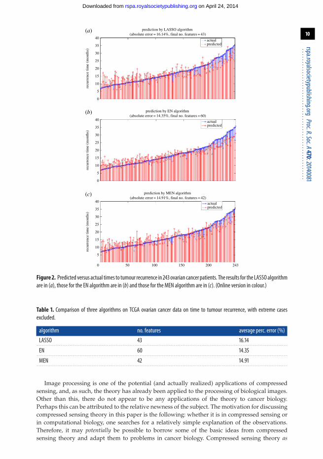
The MEN algorithm was applied to the TCGA ovarian cancer data [29] to predict the timeto tumour recurrence. Specifically, both times to tumour recurrence as well as expression levelsfor 12 042 genes are available for 283 patients. Out of these, 40 patients whose tumours recurredbefore 210 days or after 1095 days were excluded from the study as being ‘extreme’ cases. Theremaining 243 samples were analysed using MEN with recursive feature elimination (RFE). Theresults are shown in figure 2. The number of features and the average percentage error in absolutevalue are shown in table 1.

3. Compressed sensingIn recent years, there have been several results that are grouped under the general heading of‘compressed sensing’ or ‘compressive sensing’. Both expressions are in use, but ‘compressedsensing’ is used in this paper. The problem can be roughly stated as follows: suppose x ∈R

n

is an unknown vector but with known structure; is it possible to determine x either exactlyor approximately by taking m� n linear measurements of x? The area of research that goesunder this broad heading grew spectacularly during the first decade of the new millennium.5

As summarized in the introduction of the paper [31], the impetus for recent work in this area wasthe desire to find algorithms for data compression that are ‘universal’ in the sense of being non-adaptive (i.e. do not depend on the data). In the original papers in this area, the results and proofswere a mixture of sampling, signal transformation (time domain to frequency domain and viceversa), randomness, etc. However, as time went on, the essential ingredients of the approach wereidentified, thus leading to a very streamlined theory that clearly transcends its original applicationdomains of image and signal processing.

5In Davenport et al. [30], it is suggested that a precursor of compressed sensing can be found in a paper that dates back to1795!



10


...................................................

prediction by LASSO algorithm (absolute error = 16.14%, final no. features = 43)

40actualpredicted

actualpredicted

actualpredicted

35

30

25

20

recu

rren

ce ti

me

(mon

ths)

15

10

5

0

40

35

30

25

20

recu

rren

ce ti

me

(mon

ths)

15

10

5

0

40

35

30

25

20

recu

rren

ce ti

me

(mon

ths)

15

10

5

0 50 100 150 200 243

prediction by EN algorithm (absolute error = 14.35%, final no. features = 60)

prediction by MEN algorithm (absolute error = 14.91%, final no. features = 42)

(b)

(a)

(c)

Figure 2. Predicted versus actual times to tumour recurrence in 243 ovarian cancer patients. The results for the LASSO algorithmare in (a), those for the EN algorithm are in (b) and those for the MEN algorithm are in (c). (Online version in colour.)

Table 1. Comparison of three algorithms on TCGA ovarian cancer data on time to tumour recurrence, with extreme casesexcluded.

algorithm no. features average perc. error (%)

LASSO 43 16.14. . . . . . . . . . . . . . . . . . . . . . . . . . . . . . . . . . . . . . . . . . . . . . . . . . . . . . . . . . . . . . . . . . . . . . . . . . . . . . . . . . . . . . . . . . . . . . . . . . . . . . . . . . . . . . . . . . . . . . . . . . . . . . . . . . . . . . . . . . . . . . . . . . . . . . . . . . . . . . . . . . . . . . . . . . . . . . . . . . . . . . . . . . . . . . . . . . . . . . . . . .

EN 60 14.35. . . . . . . . . . . . . . . . . . . . . . . . . . . . . . . . . . . . . . . . . . . . . . . . . . . . . . . . . . . . . . . . . . . . . . . . . . . . . . . . . . . . . . . . . . . . . . . . . . . . . . . . . . . . . . . . . . . . . . . . . . . . . . . . . . . . . . . . . . . . . . . . . . . . . . . . . . . . . . . . . . . . . . . . . . . . . . . . . . . . . . . . . . . . . . . . . . . . . . . . . .

MEN 42 14.91. . . . . . . . . . . . . . . . . . . . . . . . . . . . . . . . . . . . . . . . . . . . . . . . . . . . . . . . . . . . . . . . . . . . . . . . . . . . . . . . . . . . . . . . . . . . . . . . . . . . . . . . . . . . . . . . . . . . . . . . . . . . . . . . . . . . . . . . . . . . . . . . . . . . . . . . . . . . . . . . . . . . . . . . . . . . . . . . . . . . . . . . . . . . . . . . . . . . . . . . . .

Image processing is one of the potential (and actually realized) applications of compressedsensing, and, as such, the theory has already been applied to the processing of biological images.Other than this, there do not appear to be any applications of the theory to cancer biology.Perhaps this can be attributed to the relative newness of the subject. The motivation for discussingcompressed sensing theory in this paper is the following: whether it is in compressed sensing orin computational biology, one searches for a relatively simple explanation of the observations.Therefore, it may potentially be possible to borrow some of the basic ideas from compressedsensing theory and adapt them to problems in cancer biology. Compressed sensing theory as



11


...................................................

it currently stands cannot directly be applied to the analysis of biological datasets, because thefundamental assumption in compressed sensing theory is that one is able to choose the so-calledmeasurement matrix, called A throughout this paper. Note that, in statistics, the matrix A isoften referred to as the ‘design’ matrix. However, in biological (and other) applications, themeasurement matrix is given, and one does not have the freedom to change it. Nevertheless, thedevelopments in this area are too important to be ignored by computational biologists. The hopeis that, by understanding the core arguments of compressed sensing theory, the computationalbiology community would be able to adapt the theory for its application domain. In parallel,those who are well versed in compressed sensing theory can start thinking about how the basicarguments can be modified to the case where the measurement matrix is specified, and cannotbe chosen.

The major developments in this area are generally associated with the names of Candès,Donoho, Romberg and Tao, though several other researchers have also made importantcontributions. See Donoho [31] for one of the earliest comprehensive papers, as well Donoho[32], Candés [33], Candés & Tao [34,35], Candés & Plan [36], Romberg [37] and Cohen et al. [38].The survey paper [30] and a recent paper [16] contain a wealth of bibliographic references thatcan be followed up by interested readers.

We begin by introducing some notation. Suppose m, n, k are given integers, with n≥ 2k. Forconvenience, we denote the set {1, . . . , n} by N throughout. For a given vector x ∈R

n, let supp(x)denote its support, that is, supp(x)= {i : xi �= 0}. Let, Σk = {x ∈R

n : |supp(x)| ≤ k}. Thus, Σk denotesthe set of ‘k-sparse’ vectors in R

n, or, in other words, the set of n-dimensional vectors that havek or fewer non-zero components. For each vector x ∈R

n, integer k < n and norm ‖ · ‖ on Rn, the

symbol σk(x, ‖ · ‖) denotes the distance from x to Σk, that is,

σk(x, ‖ · ‖)= inf{‖x− z‖ : z ∈Σk}.The quantity σk(x, ‖ · ‖) is called the ‘sparsity measure’ of the vector x of order k with respect to thenorm ‖ · ‖. It is obvious that σk(x, ‖ · ‖) depends on the underlying norm. However, if ‖ · ‖ is oneof the �p-norms, then it is easy to compute σk(x, ‖ · ‖). Specifically, given k, let Λ0 denote the indexset corresponding to the k-largest components of x in magnitude, and let xΛc

0denote the vector

that results by replacing the components of x in the set Λ0 by zeros. (It is convenient to think ofxΛc as an element of R

n rather than an element of Rn−k.) Then, whenever p ∈ [1,∞], it is easy to

see thatσk(x, ‖ · ‖p)= ‖xΛc

0‖p.

Next, the so-called ‘restricted isometry property’ (RIP) is introduced. Note that, in somecases, the RIP can be replaced by a weaker property known as the ‘null space property’ [38].However, the objective of this paper is not to present the most general results, but rather to presentreasonably general results that are easy to explain. So the exposition below is confined to the RIP.

Definition 3.1. Suppose A ∈Rm×n. We say that A satisfies the RIP of order k with constant δk if

(1− δk)‖u‖22 ≤ 〈u, Au〉 ≤ (1+ δk)‖u‖22, ∀u ∈Σk. (3.1)

So the matrix A has the RIP of order k with constant 1− δk if the following propertyholds: for every choice of k or fewer columns of A (say the columns in the set J⊆N , where|J| ≤ k), the spectrum of the symmetric matrix At

JAJ lies in the interval [1− δk, 1+ δk], where

AJ ∈Rm×|J| denotes the submatrix of A consisting of all rows and the columns corresponding

to the indices in J.If integers n, k are specified, the integer m has to be sufficiently large in order for the matrix A

to satisfy the RIP.

Theorem 3.2 (Davenport et al. [30, theorem 1.4]). Suppose A ∈Rm×n satisfies the RIP or order 2k

with constant δ2k ∈ (0, 1/2]. Then,

m≥ ck log(n

k

)= ck(log n− log k), (3.2)



12


...................................................

where

c= 1

2 log(√

24+ 1)≈ 0.28.

Next, we state some of the main known results in compressed sensing. The theorem statementbelow corresponds to Candès [33, theorem 1.2] and Davenport et al. [30, theorem 1.9].

Theorem 3.3. Suppose A ∈Rm×n satisfies the RIP of order δ2k with constant δ2k <

√2− 1, and that

y=Ax+ η for some x ∈Rn and η ∈R

m with ‖η‖2 ≤ ε. Define

x̂= argminz∈Rn

‖z‖1 s.t. ‖y− Az‖2 ≤ ε. (3.3)

Then,

‖x̂− x‖2 ≤C0σk(x, ‖ · ‖1)√

k+ C2ε, (3.4)

where

C0 = 21+ (√

2− 1)δ2k

1− (√

2+ 1)δ2kand C2 = 4

√1+ δ2k

1− (√

2+ 1)δ2k. (3.5)

The formula for C2 is written slightly differently from that in Davenport et al. [30, theorem 1.9]but is equivalent to it.

Corollary 3.4. Suppose A ∈Rm×n satisfies the RIP of order δ2k with constant δ2k <

√2− 1, and that

y=Ax+ η for some x ∈Σk and η ∈Rm with ‖η‖2 ≤ ε. Define

x̂= argminz∈Rn

‖z‖1 s.t. ‖y− Az‖2 ≤ ε. (3.6)

Then,‖x̂− x‖2 ≤C2ε, (3.7)

where C2 is defined in (3.5).

Corollary 3.5. Suppose A ∈Rm×n satisfies the RIP of order δ2k with constant δ2k <

√2− 1, and that

y=Ax for some x ∈Σk. Let, A−1(y) := {z ∈Rn : y=Az} and define

x̂= argminz∈A−1(y)

‖z‖1. (3.8)

Then, x̂= x.

Both corollaries follow readily from the bound (3.4). Note that if x ∈Σk, then σk(x, ‖ · ‖1)= 0.Thus, (3.4) implies that ‖x̂− x‖2 ≤C2ε if there is measurement error, and ‖x̂− x‖2 = 0, i.e. thatx̂= x, if there no measurement error.

Corollary 3.4 is referred to as the ‘near ideal’ property of the LASSO algorithm. Suppose thatx ∈Σk so that x is k-sparse. Let S denote the support of x, and let AS ∈R

m×|S| denote the submatrixof A consisting of the columns corresponding to indices in S. If an ‘oracle’ knew not only the sizeof S, but the set S itself, then the oracle could compute x̂ as

x̂oracle = (ATSAS)−1AT

Sy= x+ (ATSAS)−1AT

Sη.

Then, the error would be

‖x̂oracle − x‖2 = ‖(ATSAS)−1AT

Sη‖2 ≤ const · εfor some appropriate constant. On the other hand, if x ∈Σk, then σk(x, ‖ · ‖1)= 0, and the right-hand side of (3.4) reduces to (3.7), that is,

‖x̂− x‖2 ≤C2ε.

The point therefore is that, if the matrix A satisfies RIP, and the constant δ2k satisfies the‘compressibility condition’ δ2k <

√2− 1, then the mean-squared error of the solution to the



13


...................................................

optimization problem (3.6) is bounded by a fixed (or ‘universal’) constant times the error boundachieved by an ‘oracle’ that knows the support of x.

It should be noted that there is a parallel, and closely related, set of papers that study thefollowing problem: given a matrix A ∈R

m×n, a feature vector x that is known to be k-sparsebut otherwise unknown, and a random measurement error w assuming values in R

m, supposeone is given the noise-corrupted measurement y=Ax+ w. To recover x from y, one solves theminimization problem

x∗ = argminz∈Rn

‖y− Az‖22 + λ‖z‖1, (3.9)

where l is a user-specified penalty weight. What, if any, is the relationship between x∗ and x?It is easy to see that the objective function in (3.9) is just the Lagrangian associated with theconstrained objective function in (3.3). Specifically, if λ is sufficiently large, then large values of‖z‖1 are penalized, and the problem in (3.9) begins to resemble that in (3.3). Of course, the boundε on the magnitude of the noise is not present in the problem formulation (3.9). In Candès & Plan[36] and Negabhan et al. [16], the above problem is analysed, and probabilistic (with respect tothe random noise w) bounds analogous to (3.7) are derived. Indeed, [16] contains a very generaltheory wherein the �2-norm of y− Az is replaced by an arbitrary convex function, and the �1-normis replaced by any decomposable norm.

The advantage of the above theorem statements, which are taken from Candès [33] andDavenport et al. [30], is that the role of various conditions is clearly delineated. For instance, theconstruction of a matrix A ∈R

m×n that satisfies the RIP is usually achieved by some randomizedalgorithm. In Candès & Tao [34, theorem 1.5], such a matrix is constructed by taking the columnsof A to be samples of i.i.d. Gaussian variables. In Achlioptas [39], Bernoulli processes are usedto construct A, which has the advantage of ensuring that all elements aij have just three possiblevalues, namely 0,+1,−1. A simple proof that the resulting matrices satisfy the RIP with highprobability is given in Baraniuk et al. [40]. Neither of these construction methods is guaranteedto generate a matrix A that satisfies RIP. Rather, the resulting matrix A satisfies RIP with someprobability, say ≥ 1− γ1. The probability γ1 that the randomized method may fail to generatea suitable A matrix can be bounded using techniques that have nothing to do with the abovetheorem. Similarly, in case the measurement matrix A satisfies the RIP but the measurementnoise η is random, then it is obvious that theorem 3.3 holds with probability ≥ 1− γ2, whereγ2 is a bound on the tail probability Pr{‖η‖2 > ε}. Again, the problem of bounding this tailprobability has nothing to do with theorem 3.3. By combining both estimates, it follows that ifthe measurement matrix A is generated through randomization, and if the measurement noise isalso random, then theorem 3.3 holds with probability ≥ 1− γ1 − γ2.

Observe that the optimization problem (3.6) is

minz‖z‖1 s.t. ‖y− Az‖2 ≤ ε.

This raises the question as to whether the �1-norm can be replaced by some other norm ‖ · ‖P thatinduces some other form of sparsity, for example group sparsity. If some other norm is used inplace of the �1-norm, does the resulting algorithm display near-ideal behaviour, as does LASSO?In other words, is there an analogue of theorem 3.3 if ‖ · ‖1 is replaced by another penalty ‖ · ‖P?In joint work with Ahsen [41], the author has proved a very general theorem to the followingeffect: whenever the penalty norm is ‘decomposable’ and the measurement matrix A satisfies a‘group RIP’, the corresponding algorithm has near-ideal behaviour provided a ‘compressibilitycondition’ is satisfied. The result is described in brief.

Let G = {G1, . . . , Gg} be a partition of N = {1, . . . , n}. This implies that the sets Gi are pairwisedisjoint. If S⊆ {1, . . . , g}, define GS :=∪i∈SGi. Let k be some integer such that k≥maxi |Gi|.A subset Λ⊆N is said to be S-group k-sparse if Λ=GS and |GS| ≤ k, and group k-sparse if it isS-group k-sparse for some set S⊆ {1, . . . , g}. The symbol GkS⊆ 2N denotes the collection of groupk-sparse sets.

Suppose ‖ · ‖P : Rn→R+ is some norm. The next definition builds on an earlier definition from

Negabhan et al. [16].



14


...................................................

Definition 3.6. The norm ‖ · ‖P is decomposable with respect to the partition G if the followingis true: whenever u, v ∈R

n are group k-sparse with support sets Λu ⊆GS1 , Λv ⊆GS2 and the setsS1, S2 are disjoint, it is true that

‖u+ v‖P = ‖u‖P + ‖v‖P. (3.10)

By adapting the arguments in Negabhan et al. [16], it can be shown that the GL norm used in(2.7), namely

‖x‖GL :=g∑

l=1

√nl‖xGl‖2,

and the SGL norm used in (2.8), namely

‖x‖SL :=g∑

l=1

[(1− μ)‖xGl‖1 + μ‖xGl‖2],

are both decomposable.Next, the notion of RIP is extended to groups.

Definition 3.7. A matrix A ∈Rm×n is said to satisfy the group RIP of order k with constants ρk, ρ̄k

if

0 < ρk ≤ minΛ∈GkS

minsupp(z)⊆Λ

‖Az‖22‖z‖22

≤ maxΛ∈GkS

maxsupp(z)⊆Λ

‖Az‖22‖z‖22

≤ ρ̄k. (3.11)

We define δk := (ρ̄k − ρk)/2 and introduce some constants

c := minΛ∈GkS

minxΛ �=0

‖xΛ‖P‖xΛ‖2

and d := maxΛ∈GkS

maxxΛ �=0

‖xΛ‖P‖xΛ‖2

. (3.12)

With these definitions, the following theorem can be proved.

Theorem 3.8. Suppose A ∈Rm×n satisfies the group RIP property of order 2k with constants (ρ2k, ρ̄2k),

respectively, and let δ2k = (ρ̄2k − ρ2k)/2. Suppose x ∈Rn and that y=Ax+ η, where ‖η‖2 ≤ ε. Suppose

that the norm ‖ · ‖P is decomposable, and define

x̂= argminz∈Rn

‖z‖P s.t. ‖y− Az‖2 ≤ ε. (3.13)

Suppose that the compressibility condition

δ2k <cρkd

(3.14)

is satisfied. Then,

‖x̂− x‖P ≤ 21− r

[2(1+ r)σ + ζ ε] (3.15)

and

‖x̂− x‖2 ≤ 2c(1− r)

[2(1+ r)σ + ζ ε], (3.16)

where σ is shorthand for the sparsity index

σ = σk,G(x, ‖ · ‖P) := minΛ∈GkS

‖x− xΛ‖P = minΛ∈GkS

‖xΛc0‖P (3.17)

and

r := δ2kdcρk

and ζ := 2d√

ρ̄k

ρk

, (3.18)

and c, d are defined in (3.12).

In the above theorem, (3.14) replaces the compressibility condition δ2k <√

2− 1 of theorem 3.3.The resemblance of (3.16) to (3.4) is obvious. Consequently, (3.16) can be readily interpreted asstating that minimizing the decomposable norm ‖ · |‖P leads to near-ideal behaviour.



15


...................................................

Figure 3. A linearly separable dataset. (Online version in colour.)

4. Classification methodsThe basic problem of classification can be stated as follows: suppose we are given a collectionof labelled vectors (xi, yi), i= 1, . . . , m, where each xi ∈R

n is viewed as a row vector and eachyi ∈ {−1, 1}. For future use, define

M1 := {i : yi = 1} and M2 = {i : yi =−1}.The objective of (two-class) classification is to find a discriminant function f : R

n→R such that f (xi)has the same sign as yi for all i, or equivalently yi · sign ( f (xi))= 1 for all i. In the present context,the objective is not merely to find such a discriminant function, but, rather, to find one that usesrelatively few features.

In many ways, classification is an easier problem than regression, because the sole criterionis that the discriminant function f (xi) should have the same sign as the label yi for each i.Thus, if f is a discriminant function, so is αf for every positive constant α, and, more generally,so is any function φ( f ) whenever φ is a so-called ‘first- and third-quadrant function’, i.e.where φ(u) > 0 when u > 0 and φ(u) < 0 when u < 0. This gives us great latitude in choosing adiscriminant function.

(a) The �2-norm support vector machineThis section is devoted to the well-known SVM, first introduced in Cortes & Vapnik [42], whichis among the most successful and most widely used tools in machine learning. To distinguishthis algorithm from its variants, it is referred to here as the �2-norm SVM, for reasons that willbecome apparent.

A given set of labelled vectors {(xi, yi), xi ∈Rn, yi ∈ {−1, 1}} is said to be linearly separable if

there exist a ‘weight vector’ w ∈Rn (viewed as a column vector) and a ‘threshold’ θ ∈R such that

f (x)= xw− θ serves as a discriminant function. Equivalently, the dataset is linearly separable ifthere exist a weight vector w ∈R

n and a threshold θ ∈R such that

xiw > θ ∀i ∈M1 and xiw < θ ∀i ∈M2.

To put it yet another way, given a weight w and a threshold θ , define H=H(w, θ ) by

H := {x ∈Rn : xw− θ = 0}.H+ := {x ∈R

n : xw− θ > 0}, H− := {x ∈Rn : xw− θ < 0}.

The dataset is linearly separable if there exists a hyperplane H such that xi ∈H+ ∀i ∈M1 andxi ∈H− ∀i ∈M2.

The situation can be depicted as in figure 3a, in which the dots on either side of the dashed linerepresent the two classes. It is clear that linear separability is not affected by swapping the classlabels.

It is easy to see that, if there exists one hyperplane that separates the two classes, there existinfinitely many such hyperplanes. The question therefore arises as to which of these choices isthe best. The SVM introduced in Cortes & Vapnik [42] chooses the separating hyperplane such



16


...................................................

Figure 4. Optimal separating hyperplane. (Online version in colour.)

that the nearest point to the hyperplane within each class is as far as possible from it. In the originalSVM formulation, the distance to the hyperplane is measured using the Euclidean or �2-norm. Toillustrate the concept, the same dataset as in figure 3 is shown again in figure 4, with the ‘optimal’separating hyperplane, and the closest points to it within the two classes shown as hollow circles.

In symbols, the SVM is obtained by solving the following optimization problem:

maxw,θ

mini

infv∈H‖v − xi‖.

An equivalent formulation of the SVM is obtained by observing that the distance of the separatinghyperplane to the nearest points is given by c/‖w‖, where

c := mini∈M1

|yi(xiw− θ )| = min

i∈M2

|yi(xiw− θ )|,

where the equality of the two terms follows from the manner in which the separating hyperplaneis chosen. Moreover, the optimal hyperplane is invariant under scale change, that is, multiplyingw and θ by a positive constant. Therefore, there is no loss of generality in taking the constant c toequal one. With this rescaling, the problem at hand becomes the following:

minw‖w‖ s.t. xiw≥ 1∀i ∈M1 and xiw≤−1∀i ∈M2. (4.1)

This is the manner in which the SVM is implemented nowadays in most software packages.The original SVM formulation presupposes that the dataset is linearly separable. It is easy to

determine whether or not a given dataset is linearly separable, because that is equivalent to thefeasibility of a linear programming problem. This naturally raises the question of what is to bedone in case the dataset is not linearly separable. One way to approach the problem is to choosea hyperplane that misclassifies the fewest number of points. While appealing, this approach isimpractical, because it is known that this problem is NP-hard; see Höffgen et al. [43] and Natarajan[15]. A tractable approach is to replace this problem by its convex relaxation. We will return to thisissue when we discuss �1-norm SVMs.

An alternative approach to guarantee that the data are linearly separable can be obtained usingVapnik–Chervonenkis theory [44,45]. Suppose that the n vectors x1, . . . , xn do not lie on an (p− 1)-dimensional hyperplane in R

p. In such a case, whenever p≥ n− 1, the dataset is linearly separablefor every one of the 2n ways of assigning labels to the n vectors. This result suggests that, if a givendataset is not linearly separable, it can be made so by increasing the dimension of the data vectorsxi, for instance, by including not just the original components but also their higher powers. Thisis the rationale behind so-called ‘higher order’ SVMs, or, more generally, kernel-based classifiers(e.g. Cristianini & Shawe-Taylor [46] and Schölkopf & Smola [47]).

If the norm in (4.1) is the �2-norm, then the minimization problem (4.1) is a quadraticprogramming problem, which can be solved efficiently for extremely large datasets. Moreover,the introduction of new data points does not alter the optimal hyperplane, unless one of thenew data points is closer to the hyperplane than the earlier closest points. This is illustrated infigure 5, which contains exactly the same vectors as in figure 4, plus two more. The optimal



17


...................................................

Figure 5. Insensitivity of optimal separating hyperplane to additional samples. (Online version in colour.)

hyperplane remains the same. For all these reasons, the SVM offers a very attractive approachto finding a classifier in situations where the number of features is smaller than the number ofsamples. On the other hand, generically the optimal weight vector has all non-zero components,which is undesirable when the number of samples m is too large, even if m < n. To overcome thisproblem, an approach known as RFE is suggested in Guyon et al. [48]. This consists of solving theSVM problem (4.1), identifying the component of the weight vector with the smallest magnitude,discarding it, re-solving the problem and repeating. Though it is claimed in Guyon et al. [48] thatthe method works well on a leukaemia dataset, in general RFE applied to the traditional �2-normSVM displays rather erratic behaviour.

(b) The �1-norm support vector machineAs we have seen, in biological applications, the number of features (the dimension of thevectors xi) is a few orders of magnitude larger than the number of samples (the number ofvectors). In such a case, because of the results in Wenocur & Dudley [44], linear separability isnot an issue. However, in general, every component of the optimal weight vector w is non-zero.This means that a classifier uses every single feature in order to discriminate between the classes.Clearly, this is undesirable. The original SVM formulation presupposes that the dataset is linearlyseparable. If the data are not linearly separable, then as shown in Höffgen et al. [43] and Natarajan[15], the problem of finding a hyperplane that misclassifies the fewest points is NP-hard. Analternative approach is to formulate a convex relaxation of this NP-hard problem by introducingslack variables into the constraints in (4.1), and then minimizing an appropriate norm of the vectorof slack variables. Finally, in many problems, the consequences of misclassification might notbe symmetric. A false positive (labelling a sample as positive when in fact it is negative) mighthave far more, or far less, severe consequences than a false negative. In this section, we presenta problem formulation that addresses all of these issues. This problem formulation combines theideas in two papers, namely [49,50].

If we choose a particular norm ‖ · ‖ to measure distances in ‘feature space’, then distances in‘weight space’ should be measured using the so-called dual norm, defined by

‖w‖d := sup‖x‖≤1

|xw|.

In particular, if we measure distances in feature space using the �1-norm, then distances in weightspace should be measured using its dual, which is the �∞-norm. With this observation, theproblem can be formulated as follows:

minw,θ ,y,z

(1− λ)

[ m1∑i=1

yi +m2∑i=1

zi

]+ λ max

1≤i≤n|wi| s.t.

xiw− θ + yi ≥ 1∀i ∈M1, xiw− θ − zi ≤−1∀i ∈M2,

y≥ 0m1 and z≥ 0m2 .

⎫⎪⎪⎪⎪⎪⎬⎪⎪⎪⎪⎪⎭

(4.2)



18


...................................................

This can be converted to

minw,θ ,y,z

(1− λ)

[ m1∑i=1

yi +m2∑i=1

zi

]+ λv s.t.

xiw− θ + yi ≥ 1∀i ∈M1, xiw− θ − zi ≤−1∀i ∈M2,

y≥ 0m1 , z≥ 0m2 and v ≥wi ∀i, v ≥−wi ∀i.

⎫⎪⎪⎪⎪⎪⎬⎪⎪⎪⎪⎪⎭

(4.3)

This is clearly a linear programming problem. In this formulation, λ is a ‘small’ constant in (0, 1),much closer to 0 than it is to 1. Suppose that the original dataset is linearly separable, and let w∗, θ∗denote a solution to the optimization problem in (4.1), where ‖w‖d replaces ‖w‖. Then the choice

w=w∗, θ = θ∗, y= 0m1 and z= 0m2

is certainly feasible for the optimization problem (4.2). Moreover, if λ is sufficiently small, anyreduction in ‖w‖d achieved by violating the linear separation constraints (i.e. permitting someyi or zi to be positive rather than zero) is offset by the increase in the term (1− λ)‖(y, z)‖. It istherefore clear that, if the dataset is linearly separable, there exists a critical value λ0 > 0 such that,for all λ < λ0, the optimization problem (4.2) has (w∗, θ , 0m1 , 0m2 ) as a solution. On the other hand,the optimization problem (4.2) remains meaningful even when the data are not linearly separable.

The final aspect of the problem, as suggested in Veropoulos et al. [50], is to introduce a trade-off between false positives and false negatives. In this connection, it is worthwhile to recall thedefinitions of the accuracy, etc. of a classifier. Given a discriminant function f (·), define

C1 := {i ∈M : f (xi) > 0} and C2 := {i ∈M : f (xi) < 0}.

Thus, C1 consists of the samples that are assigned to class 1 by the classifier, while C2 consists ofthe samples that are assigned to class 2. Then, this leads to the array shown below

C1 C2M1 TP FNM2 FP TN

In the above array, the entries TP, FN, FP and TN stand for ‘true positive’, ‘false negative’, ‘falsepositive’ and ‘true negative’, respectively.

Definition 4.1. With the above definitions, we have

Se= TPTP+ FN

= |C1 ∩M1||M1|

, (4.4)

Sp= TNFP+ TN

= |C2 ∩M2||M2|

(4.5)

and Ac= TP+ TNTP+ TN+ FP+ FN

= |C1 ∩M1| + |C2 ∩M2||M1| + |M2|

, (4.6)

where Se, Sp and Ac stand for the sensitivity, specificity and accuracy, respectively.

All three quantities lie in the interval [0, 1]. Moreover, accuracy is a convex combination ofsensitivity and specificity. In particular,

Ac= Se · |M1||M1| + |M2|

+ Sp · |M2||M1| + |M2|

.

Therefore,

min{Se, Sp} ≤Ac≤max{Se, Sp}.

Also, the accuracy of a classifier will be roughly equal to the sensitivity if M1 is far larger thanM2, and roughly equal to the specificity if M2 is far larger than M1.



19


...................................................

In many classification problems, the consequences of misclassification are not symmetric. Tocapture these kinds of considerations, another parameter α ∈ (0, 1) is introduced, and the objectivefunction in the optimization problem (4.2) is modified by making the substitution

m1∑i=1

yi +m2∑i=1

zi← α

m1∑i=1

yi + (1− α)m2∑i=1

zi,

where we adopt the computer science notation← to mean ‘replaces’. If α= 0.5, then both falsepositives and false negatives are weighted equally. If α > 0.5, then there is greater emphasison correctly classifying the vectors in M1, and the reverse if α < 0.5. With this final problemformulation, the following desirable properties result:

— the problem is a linear programming problem and is therefore tractable even forextremely large values of n, the number of features;

— the formulation can be applied without knowing beforehand whether or not the datasetis linearly separable;

— the formulation provides for a trade-off between false positives and false negatives; and— most important, the optimal weight vector w has at most m non-zero entries, where m is

the number of samples. Hence, the classifier uses at most m out of the n features.

For these reasons, the �1-norm SVM forms the starting point for our further research intoclassification.

Until now, the discussion has been on two-class classification. The SVM framework does notextend to multi-class classification very readily. For one thing, when there are only two classes,it does not matter which class is labelled ‘positive’ and which is labelled ‘negative’. On the otherhand, when there are multiple classes, it is necessary to distinguish between two cases: in thefirst, there is a natural ordering among the class labels. For instance, if a patient’s response is tobe categorized as poor, fair, good, very good and excellent, the ordering is clear. In the second,there is no natural ordering, for example, if one wishes to assign a breast cancer tumour into oneof the four subtypes mentioned above. The paper [51] is among the more popular methods formulti-class SVM.

(c) Some applications of support vector machines to cancerIn contrast with sparse regression, there are many applications of sparse classification methods tocancer biology. A search of the Pubmed database of the National Library of Medicine, USA, withthe string ‘SVM cancer’ returns several hundred results. The vast majority of these papers presentapplications where human experts pare the hundreds or even thousands of measured features toa small subset, to which a standard �2-norm SVM is applied. In other words, though the rawnumber of measured features is very high, the actual number of features used by the SVM issmaller than the number of samples. In principle, the �1-norm SVM can be applied to the originalfeature set to choose the most predictive features out of the overall feature set. But for the mostpart, existing applications appear to leave the task of feature selection to human experts and notto the algorithm. The fraction of SVM applications that exploit the feature selection property ofthe �1-norm SVM is quite small. Two reasons, not mutually exclusive, can be proposed to explainthis. First, the users might simply be unfamiliar with the �1-norm SVM methodology. Second,the users might believe that a purely data-driven approach might result in a feature set whosebiological significance is unclear.

The paper [48] that introduces the technique of RFE to the SVM algorithm studies theapplication of the technique to leukaemia. It is shown that the SVM–RFE method eventually leadsto just two features being retained. However, several authors report that the performance of theSVM–RFE approach is in general somewhat erratic. It would appear therefore that the datasetstudied in Guyon et al. [48] is particularly amenable to the use of this technique. An excellentreview of several applications of SVMs to ovarian cancer can be found in Sabatier et al. [52].



20


...................................................

Other examples of ovarian cancer applications include Han et al. [53], in which 322 samples areanalysed to generate a 349-gene biomarker panel which performs very well, but when the 349genes are reduced to 18 genes the performance on the test data is poor; Denkert et al. [54], inwhich a 300-gene ovarian carcinoma index is constructed on the basis of 80 samples, which isthen tested on 118 samples; and Hartmann et al. [55], in which a panel of 14 genes is identified todifferentiate between early relapse and late-stage relapse. Yet, these papers ignore the result fromWenocur & Dudley [44], which states that if the number of features used is in excess of the numberof samples in the training data, then generically an SVM can achieve 100% accuracy, sensitivityand specificity on the training data, irrespective of the assignment of labels to the samples. Asneither Han et al. [53] nor Denkert et al. [54] reports such a phenomenon, it is unclear whetherthese papers have implemented the SVM algorithm accurately.

As illustrations of applications to other forms of cancer, one can mention: Sabatier et al. [56], inwhich a 368-gene expression signature is trained on 2145 basal breast cancer samples, and thentested on another set of 2034 samples, with the aim of predicting the patient’s prognosis; andKlement et al. [57], in which seven features were selected by human experts to study 399 NSCLCpatients. As an example of using not just SVM but also RFE, one can cite Yang et al. [58], in whichthe efficacy of drug candidates against hepatocellular carcinoma (liver cancer) is studied. As theefficacy of drug candidates is actually a real number between 0 and 1, the authors discretize theefficacy into two bins: [0, 0.4] and [0.6, 1]. Apparently, their only motivation is to make the problemfit into the SVM framework. Therefore, it would be worthwhile to apply sparse regressiontechniques (as opposed to sparse classification) to such problems. Finally, an application of themulti-class SVM methodology of Crammer & Singer [51] is found in Huang et al. [59].

(d) The lone star algorithmAs pointed out in §4, both the traditional �2-norm SVM and the �1-norm SVM can be used fortwo-class classification problems. When the number of samples m is far larger than the number offeatures n, the traditional SVM performs very satisfactorily, whereas the �1-norm SVM of Bradley& Mangasarian [49] is to be preferred when m < n. Moreover, the �1-norm SVM is guaranteedto use no more than m features. However, in many biological applications, even m features aretoo many. Biological measurements suffer from poor repeatability. Therefore, a classifier thatuses fewer features would be far preferable to one that uses more features. In this section, wepresent a new algorithm for two-class classification that often uses far fewer than m features, thusmaking it very suitable for biological applications. The algorithm combines the �-norm SVM ofBradley & Mangasarian [49], RFE of Guyon et al. [48] and stability selection of Meinshausen &Bühlmann [60]. A preliminary version of this algorithm was reported in Ahsen et al. [61]. Notethat Li et al. [62] introduces an algorithm known as SVM–T–RFE that contains some similarities tothis algorithm.

The algorithm is as follows:

(1) Choose at random a ‘training set’ of samples of size k1 from M1 and size k2 from M2,such that kl ≤ml/2 and k1, k2 are roughly equal. Repeat this choice s times, where s isa ‘large’ number. This generates s different ‘training sets’, each of which consists of klsamples from Ml, l= 1, 2.

(2) For each randomly chosen training set, compute a corresponding optimal �1-normSVM using the formulation (4.2). This results in s different optimal weight vectors andthresholds.

(3) Let k denote the average number of non-zero entries in the optimal weight vector acrossall randomized runs. Average all s optimal weight vectors and thresholds, retain thelargest k components of the averaged weight vector and corresponding feature set, andset the remaining components to zero. This results in reducing the number of featuresfrom the original n to k.



21


...................................................

(4) Repeat the process with the reduced feature set, but the originally chosen randomlyselected training samples, until no further reduction is possible in the number of features.This determines the final set of features to be used.

(5) Once the final feature set is determined, carry out twofold cross validation by dividingthe data s times into a training set of k1, k2 randomly selected samples and assessingthe performance of the resulting �1-norm classifier on the testing dataset, which is theremainder of the samples. Average the weights generated by the t≤ s best-performingclassifiers, where t is chosen by the user, and call that the final classifier.

When the number of features n is extremely large, an optional pre-processing step is tocompute the mean value of each of the n features for each class, and retain only those featureswherein the difference between means is statistically significant using the ‘Student’ t-test. Ourexperience is that using this optional pre-processing step does not change the final answer verymuch, but does decrease the CPU time substantially. Note that, in Li et al. [62], a weightedcombination of the weight of the �2-norm SVM and the t-test statistic is used to eliminate features.

Now some comments are in order regarding the above algorithm:

— in some applications, M1 and M2 are of comparable size, so that the size of the trainingset can be chosen to equal roughly half of the total samples within each class. However,in other applications, the sizes of the two sets are dissimilar, in which case the larger sethas far fewer of its samples used in training;

— step 1 of randomly choosing s different training sets differs from Guyon et al. [48], wherethere is only one randomized division of the data into training and testing sets;

— for each random choice of the training set, the number of non-zero entries in the optimalweight vector is more or less the same; however, the locations of non-zero entries in theoptimal weight vector vary from one run to another;

— in step 3 above, instead of averaging the optimal weights over all s runs and then retainingthe k largest components, it is possible to adopt another strategy. Rank all n indices inorder of the number of times that index has a non-zero weight in the s randomized runs,and retain the top k indices. In our experience, both approaches lead to virtually the samechoice of the indices to be retained for the next iteration;

— instead of choosing s randomized training sets right at the outset, it is possible to chooses randomized training sets each time the number of features is reduced; and

— in the final step, there is no distinction between the training and testing datasets, so thefinal classifier is run on the entire dataset to arrive at the final accuracy, sensitivity andspecificity figures.

The advantage of the above approach vis-à-vis the �2-norm SVM–RFE of Guyon et al. [48]or the SVM–T–RFE of Li et al. [62] is that the number of features reduces significantly at eachstep, and the algorithm converges in just a few steps. This is because, in the �1-norm SVM, manycomponents of the weight vector are ‘naturally’ zero and need not be truncated. By contrast, ingeneral all the components of the weight vector resulting from the �2-norm SVM will be non-zero; as a result, the features can only be eliminated one at a time, and in general the number ofiterations is equal to (or comparable to) n, the initial number of features.

The new algorithm can be appropriately referred to as the ‘�1-SVM t-test and RFE’ algorithm,where SVM and RFE are themselves acronyms as defined above. Once again taking the firstletters, we are led to the ‘second-level’ acronym ‘�1-StaR’, which can be pronounced as ‘ell-onestar’. Out of deference to our domicile, we have decided to call it the ‘lone star’ algorithm.

The lone star algorithm was applied to the problem of predicting which patients of endometrialcancer are at risk of lymph node metastasis. These results are reported elsewhere. But in brief, thesituation is the following: the endometrium is the lining of the uterus. When a patient contractsendometrial cancer, her uterus, ovaries and fallopian tubes are surgically removed. One of themajor risks run by endometrial cancer patients is that the cancer will metastasize and spread



22


...................................................

through the body via pelvic and/or para-aortic lymph nodes. The Gynecologic Oncology Grouprecommends that the patient’s pelvic and para-aortic lymph nodes should also be surgicallyremoved when the size of the tumour exceeds 2 cm in diameter. However, post-surgery analysisreveals that, even in this case, lymphatic metastasis is present in only 22% of the cases [63].

To predict the possibility of lymphatic metastasis, 1428 miRNAs were extracted from 94tumours, half with and half without metastasis. Using the lone star algorithm, 13 miRNAs wereidentified as being highly predictive. When tested on the entire training sample of 94 tumours, thelone star classifier correctly classified 41 out of 43 lymph-positive samples, and 40 out of 43 lymph-negative samples. In ongoing work, these miRNAs were measured on an independent cohort of19 lymph-negative and nine lymph-positive tumours. The classifier classified eight out of ninelymph-positive tumours correctly, and 11 out of 19 lymph-negative tumours correctly. Thus,while the specificity is not very impressive, the sensitivity is extremely good, which is preciselywhat one wants in such a situation. Moreover, using a two-table contingency analysis and theBarnard exact test, the likelihood of arriving at this assignment by pure chance (the so-calledp-value) is bounded by 0.011574. In biology, any p-value less than 0.05 is generally considered tobe significant.

5. Some topics for further researchBoth machine learning and computational biology are vast subjects, and their intersectioncontains many more topics than are touched upon in this brief article. Besides, there are othertopics in computational cancer biology that do not naturally belong to machine learning, forexample modelling tumour growth using branching processes. Therefore, the emphasis in thisarticle has been on topics that are well established in the machine learning community and arealso relevant to problems in computational cancer biology.

Until now several ‘penalty’ norms have been proposed for inducing an optimization algorithmto select structured sparse feature sets, such as GL and SGL. As pointed out in §2, availableextensions of these penalty norms to overlapping sets do not address biological networks wherethere are multiple paths from a master regulator to a final node. Any advance in this directionwould have an immediate application to computational biology.

Compressed sensing theory as discussed in §3 is based on the premise that it is possible to choosethe measurement matrix A. The available theorems in this theory are based on assumptions onthe measurement matrix, such as the RIP, or the null space property, and perhaps something evenmore general in future. In order to apply techniques from compressed sensing theory to cancerbiology, it would be necessary to modify the theory to the case where the measurement matrix isgiven, and not chosen by the user. The RIP corresponds to the assumption that in an m× n matrixA, every choice of k columns results in a nearly orthogonal set. In actual biological data, suchan assumption has no hope of being true, because the expression levels of some genes would behighly correlated with those of other genes. In Candès & Plan [36], the authors suggest that it ispossible to handle this situation by first clustering the column vectors and then choosing just oneexemplar from each cluster before applying the theory. Our preliminary attempts to apply suchan approach to ovarian cancer data [29] are not very promising, leading to RIP orders of 5 or 10—far too small to be of practical use. Thus, there is a need for the development of other heuristicsbesides clustering to extract nearly orthogonal sets of columns for actual measurement matrices.In this connection, it is worth pointing out [64] that group RIP is easier to achieve using randomprojections, as compared with RIP. However, it is not clear whether a ‘given’ A matrix is likely tosatisfy a group RIP with a sufficiently large order.

In general, it would appear that sparse regression is more advanced than sparse classification,with both well-established theoretical foundations as well as widely used algorithms in theformer. By contrast, sparse classification does not have such a wealth of results. The lone staralgorithm introduced here has performed well in several applications involving cancer data, and,at least for the moment, it appears to be the only available method to select far fewer featuresthan the size of the training set of samples. As of now, there is no theoretical justification for this



23


...................................................

observed behaviour. Recall that the �1-norm SVM is guaranteed only to choose no more featuresthan the size of the training set; but there is no reason to assume that it will use fewer. Therefore,it is certainly worthwhile to study when and why lone star and other such algorithms will proveto be effective.

Acknowledgements. The author would like to assert his deep gratitude to Prof. Michael A. White of the UTSouthwestern Medical Center, Dallas, TX, USA, for introducing him to the fascinating world of cancer biologyand for turning him into a passable imitation of a computational cancer biologist. He would also like to thankhis students Eren Ahsen, Burook Misganaw and Nitin Singh for carrying out much of the work that supportsthe theory reported here.Funding statement. This research was supported by National Science Foundation award nos. ECCS-1001643 andECCS-1306630, the Cecil & Ida Green Endowment at the UT Dallas, and by a Developmental Award from theHarold Simmons Comprehensive Cancer Center, UT Southwestern Medical Center, Dallas.

Author profile

Mathukumalli Vidyasagar is the Cecil and Ida Green (II) Professorof Systems Biology Science at the University of Texas at Dallas. Hiscurrent research interests are in the application of stochastic processesand stochastic modelling to problems in computational biology, andcontrol systems.

He was previously director of the newly created Centre for ArtificialIntelligence and Robotics (CAIR) in Bangalore, under the Ministryof Defence, Government of India, and built up CAIR into a leadingresearch laboratory, working in areas such as flight control, robotics,

neural networks and image processing. He then moved to the Indian private sector as anExecutive Vice President of India’s largest software company, Tata Consultancy Services. In thecity of Hyderabad, he created the Advanced Technology Center, an industrial R&D laboratoryof around 80 engineers, working in areas such as computational biology, quantitative finance,e-security, identity management and open source software to support Indian languages.

Vidyasagar has received a number of awards in recognition of his research contributions,including election to the Fellowship of the Royal Society in 2012, the IEEE Control Systems (Field)Award, the Rufus Oldenburger Medal of ASME and others. He is the author of 11 books andnearly 140 papers in peer-reviewed journals.

References1. Northrop RB, Connor AN. 2009 Introduction to molecular biology, genomics and proteomics for

biomedical engineers. Boca Raton, FL: CRC Press.2. Tözeren A, Byers SW. 2003 New biology for engineers and computer scientists. Englewood Cliffs,

NJ: Prentice-Hall.3. SEER. 2013 See http://seer.cancer.gov/statfacts/html/all.html.4. Siegel R, Naishadham D, Jemal A. 2013 Cancer statistics, 2013. CA Cancer J. Clin. 63, 11–30.

(doi:10.3322/caac.21166)5. Cancer Research UK. 2013 See http://www.cancerresearchuk.org.6. World Health Organization. 2013 See http://www.who.int/cancer/en/.7. Malhotra GK, Zhao X, Band H, Band V. 2010 Histological, molecular and functional subtypes

of breast cancers. Cancer Biol. Ther. 10, 955–960. (doi:10.4161/cbt.10.10.13879)8. GEO. 2013 See http://www.ncbi.nlm.nih.gov/geo/.9. COSMIC. 2013 See http://www.sanger.ac.uk/genetics/CGP/cosmic.

10. The Cancer Genome Atlas. 2013 See http://cancergenome.nih.gov/.11. International Cancer Genomics Consortium. 2013 See http://icgc.org/.12. Hastie T, Tibshirani R, Friedman J. 2011 The elements of statistical learning, 2nd edn. New York,

NY: Springer.


http://seer.cancer.gov/statfacts/html/all.html

http://dx.doi.org/doi:10.3322/caac.21166

http://www.cancerresearchuk.org

http://www.who.int/cancer/en/

http://dx.doi.org/doi:10.4161/cbt.10.10.13879

http://www.ncbi.nlm.nih.gov/geo/

http://www.sanger.ac.uk/genetics/CGP/cosmic

http://cancergenome.nih.gov/

http://icgc.org/


24


...................................................

13. Hoerl AE, Kennard RW. 1970 Ridge regression: biased estimation for nonorthogonalproblems. Technometrics 12, 55–67. (doi:10.1080/00401706.1970.10488634)

14. Tikhonov AN. 1943 On the stability of inverse problems. Doklady Akademii Nauk SSSR 39,195–198.

15. Natarajan BK. 1995 Sparse approximate solutions to linear systems. SIAM J. Comput. 24,227–234. (doi:10.1137/S0097539792240406)

16. Negabhan S, Ravikumar P, Wainwright MJ, Yu B. 2012 A unified framework for high-dimensional analysis of m-estimators with decomposable regularizers. Stat. Sci. 27, 538–557.(doi:10.1214/12-STS400)

17. Tibshirani R. 1996 Regression shrinkage and selection via the LASSO. J. R. Stat. Soc. 58,267–288.

18. Osborne MR, Presnell B, Turlach BA. 2000 On the LASSO and its dual. J. Comput. Graph. Stat.9, 319–337.

19. Zou H, Hastie T. 2005 Regularization and variable selection via the elastic net. J. R. Stat. Soc. B67, 301–320. (doi:10.1111/j.1467-9868.2005.00503.x)

20. Lee H, Flaherty P, Ji HP. 2013 Systematic genomic identification of colorectal genesdelineating advanced from early clinical stage and metastasis. BMC Med. Genomics 6, 54.(doi:10.1186/1755-8794-6-54)

21. Network TCGAR. 2012 Comprehensive molecular characterization of human colon and rectalcancer. Nature 487, 330–337. (doi:10.1038/nature11252)

22. Waldron L, Pintille M, Tsao M-S, Shepherd FA, Huttenhower C, Jurisica I. 2011 Optimizedapplication of penalized regression methods to diverse genomic data. Bioinformatics 27,3339–3406. (doi:10.1093/bioinformatics/btr591)

23. Bakin S. 1999 Adaptive regression and model selection in data mining problems. PhD thesis,The Australian National University, Canberra, Australia.

24. Lin Y, Zhang H. 2006 Component selection and smoothing in smoothing spline analysis ofvariance models. Ann. Stat. 34, 2272–2297. (doi:10.1214/009053606000000722)

25. Friedman J, Hastie T, Tibshirani R. 2010 A note on the group LASSO and sparse group LASSO.See http://www-stat.stanford.edu/∼tibs/ftp/sparse-grLASSO.pdf.

26. Simon N, Friedman J, Hastie T, Tibshirani R. 2012 A sparse group LASSO. Seehttp://www-stat.stanford.edu/∼nsimon/SGLpaper.pdf.

27. Obozinski G, Jacob L, Vert J-P. 2011 Group LASSO with overlaps: the latest group LASSOapproach. (http://arxiv.org/abs/1110.0413)

28. Jenetton R, Mairal J, Obozinski G, Bach F. 2011 Proximal methods for hierarchical sparsecoding. J. Mach. Learn. Res. 12, 2297–2334.

29. The Cancer Genome Atlas Research Network. 2011 Integrated genomic analyses of ovariancarcinoma. Nature 474, 609–615. (doi:10.1038/nature10166)

30. Davenport MA, Duarte MF, Eldar YC, Kutyniok G. 2012 Introduction to compressed sensing.In Compressed sensing: theory and applications (eds YC Eldar, G Kutyniok), pp. 1–68. Cambridge,UK: Cambridge University Press.

31. Donoho D. 2006 Compressed sensing. IEEE Trans. Inform. Theory 52, 1289–1306.(doi:10.1109/TIT.2006.871582)

32. Donoho D. 2006 For most large underdetermined systems of linear equations, the minimal�1-norm solution is also the sparsest solution. Commun. Pure Appl. Math. 59, 797–829.(doi:10.1002/cpa.20132)

33. Candès E. 2008 The restricted isometry property and its implications for compresed sensing.C. R. Acad. Sci. Paris, Ser. I 346, 589–592.

34. Candès EJ, Tao T. 2005 Decoding by linear programming. IEEE Trans. Inform. Theory 51, 4203–4215. (doi:10.1109/TIT.2005.858979)

35. Candès EJ, Tao T. 2007 The Dantzig selector: statistical estimation when p is much larger thann. Ann. Stat. 35, 2313–2351. (doi:10.1214/009053606000001523)

36. Candès EJ, Plan Y. 2009 Near ideal model selection by �1 minimization. Ann. Stat. 37, 2145–2177. (doi:10.1214/08-AOS653)

37. Romberg J. 2009 Compressive sensing by random convolution. SIAM J. Imaging Sci. 2, 1098–1128. (doi:10.1137/08072975X)

38. Cohen A, Wolfgang D, Devore R. 2009 Compressed sensing and best k-term approximation. J.Am. Math. Soc. 22, 211–231. (doi:10.1090/S0894-0347-08-00610-3)

39. Achlioptas D. 2003 Database-friendly random projections: Johnson–Lindenstraus with binarycoins. J. Comput. Syst. Sci. 66, 671–687. (doi:10.1016/S0022-0000(03)00025-4)


http://dx.doi.org/doi:10.1080/00401706.1970.10488634

http://dx.doi.org/doi:10.1137/S0097539792240406

http://dx.doi.org/doi:10.1214/12-STS400

http://dx.doi.org/doi:10.1111/j.1467-9868.2005.00503.x

http://dx.doi.org/doi:10.1186/1755-8794-6-54

http://dx.doi.org/doi:10.1038/nature11252

http://dx.doi.org/doi:10.1093/bioinformatics/btr591

http://dx.doi.org/doi:10.1214/009053606000000722

http://www-stat.stanford.edu/~tibs/ftp/sparse-grLASSO.pdf

http://www-stat.stanford.edu/~nsimon/SGLpaper.pdf

http://arxiv.org/abs/1110.0413

http://dx.doi.org/doi:10.1038/nature10166

http://dx.doi.org/doi:10.1109/TIT.2006.871582

http://dx.doi.org/doi:10.1002/cpa.20132

http://dx.doi.org/doi:10.1109/TIT.2005.858979

http://dx.doi.org/doi:10.1214/009053606000001523

http://dx.doi.org/doi:10.1214/08-AOS653

http://dx.doi.org/doi:10.1137/08072975X

http://dx.doi.org/doi:10.1090/S0894-0347-08-00610-3

http://dx.doi.org/doi:10.1016/S0022-0000(03)00025-4


25


...................................................

40. Baraniuk R, Davenport M, Devore R, Wakin M. 2008 A simple proof of the restricted isometryproperty for random matrices. Constr. Approx. 28, 253–263. (doi:10.1007/s00365-007-9003-x)

41. Ahsen ME, Vidyasagar M. 2014 Near-ideal behavior of compressed sensing algorithms.(http://arxiv.org/abs/1401.6623)

42. Cortes C, Vapnik VN. 1997 Support vector networks. Mach. Learn. 20, 273–297.(doi:10.1007/BF00994018)

43. Höffgen K-U, Simon H-U, Horn KSV. 1995 Robust trainability of single neurons. J. Comput.Syst. Sci. 50, 114–125. (doi:10.1006/jcss.1995.1011)

44. Wenocur RS, Dudley RM. 1981 Some special Vapnik–Chervonenkis classes. Discret. Math. 33,313–318. (doi:10.1016/0012-365X(81)90274-0)

45. Vidyasagar M. 2003 Learning and generalization: with applications to neural networks and controlsystems. London, UK: Springer.

46. Cristianini N, Shawe-Taylor J. 2000 Support vector machines. Cambridge, UK: CambridgeUniversity Press.

47. Schölkopf B, Smola AJ. 2002 Learning with kernels. Cambridge, MA: MIT Press.48. Guyon I, Weston J, Barnhill S, Vapnik V. 2002 Gene selection for cancer classification using

support vector machines. Mach. Learn. 46, 389–422. (doi:10.1023/A:1012487302797)49. Bradley PS, Mangasarian OL. 1998 Feature selection via concave minimization and

support vector machines. In Machine Learning: Proceedings of the 15th Int. Conf. (ICML ’98),Madison, WI, 24–27 July 1998 (ed. JW Shavlik), pp. 82–90. San Mateo, CA: Morgan Kaufmann.

50. Veropoulos K, Campbell C, Cristianini N. 1999 Controlling the sensitivity of support vectormachines. In IJCAI Workshop on Support Vector Machines. Stockholm, Sweden, 2 August 1999, pp.55–60. San Mateo, CA: Morgan Kaufmann.

51. Crammer K, Singer Y. 2001 On the algorithmic implementation of multiclass kernel-basedvector machines. J. Mach. Learn. Res. 2, 265–292.

52. Sabatier R, Finetti P, Cervera N, Birnbaum D, Bertucci F. 2009 Gene expression profilingand prediction of clinical outcome in ovarian cancer. Crit. Rev. Oncol. Hematol. 72, 98–109.(doi:10.1016/j.critrevonc.2009.01.007)

53. Han Y, Huang H, Xiao Z, Zhang W, Cao Y, Qu L, Shou C. 2012 Integrated analysis ofgene expression profiles associated with response of platinum/paclitaxel-based treatment inepithelial ovarian cancer. PLoS ONE 7, e52745. (doi:10.1371/journal.pone.0052745)

54. Denkert C et al. 2009 A prognostic gene expression index in ovarian cancer—validation acrossdifferent independent data sets. J. Pathol. 218, 273–280. (doi:10.1002/path.2547)

55. Hartmann LC et al. 2005 Gene expression profiles predict early relapse in ovarian cancerafter platinum-paclitaxel chemotherapy. Clin. Cancer Res. 11, 2149–2155. (doi:10.1158/1078-0432.CCR-04-1673)

56. Sabatier R et al. 2011 A gene expression signature identifies two prognostic subgroups of basalbreast cancer. Breast Cancer Res. Treat. 126, 407–420. (doi:10.1007/s10549-010-0897-9)

57. Klement RJ et al. 2013 Control of stereotactic body radiation therapy for early-stage non-smallcell lung cancer. Int. J. Radiat. Oncol. Biol. Phys. 88, 732–738. (doi:10.1016/j.ijrobp.2013.11.216)

58. Yang W-LR, Lee Y-E, Chen M-H, Chao K-M, Huang C-YF. 2013 In silico drug screening andpotential target identification for hepatocellular carcinoma using support vector machinesbased on drug screening result. Gene 518, 201–208. (doi:10.1016/j.gene.2012.11.030)

59. Huang L, Zhang HH, Zeng Z-B, Bushel PR. 2013 Improved sparse multi-class SVMand its application for gene selection in cancer classification. Cancer Inform. 12, 143–153.(doi:10.4137/CIN.S10212)

60. Meinshausen N, Bühlmann P. 2010 Stability selection. J. R. Stat. Soc. B 72, 417–483.(doi:10.1111/j.1467-9868.2010.00740.x)

61. Ahsen ME, Singh NK, Boren T, Vidyasagar M, White MA. 2012 A new feature selectionalgorithm for two-class classification problems and application to endometrial cancer. In Proc.IEEE Conf. Decision and Control, Maui, Hawaii, 10–13 December 2013, pp. 2976–2982. Piscataway,NJ: IEEE.

62. Li X, Peng S, Chen J, Lüc B, Zhanga H, Lai M. 2012 SVM-T-RFE: a novel gene selectionalgorithm for identifying metastasis-related genes in colorectal cancer using gene expressionprofiles. Biochem. Biophys. Res. Commun. 419, 148–153. (doi:10.1016/j.bbrc.2012.01.087)

63. Mariani A, Dowdy SC, Cliby WA, Gostout BS, Jones MB, Wilson TO, Podratz KC. 2008Prospective assessment of lymphatic dissemination in endometrial cancer: a paradigm shiftin surgical staging. Gynecol. Oncol. 109, 11–18. (doi:10.1016/j.ygyno.2008.01.023)

64. Huang J, Zhang T. 2010 The benefit of group sparsity. Ann. Stat. 38, 1978–2004.(doi:10.1214/09-AOS778)


http://dx.doi.org/doi:10.1007/s00365-007-9003-x

http://arxiv.org/abs/1401.6623

http://dx.doi.org/doi:10.1007/BF00994018

http://dx.doi.org/doi:10.1006/jcss.1995.1011

http://dx.doi.org/doi:10.1016/0012-365X(81)90274-0

http://dx.doi.org/doi:10.1023/A:1012487302797

http://dx.doi.org/doi:10.1016/j.critrevonc.2009.01.007

http://dx.doi.org/doi:10.1371/journal.pone.0052745

http://dx.doi.org/doi:10.1002/path.2547

http://dx.doi.org/doi:10.1158/1078-0432.CCR-04-1673

http://dx.doi.org/doi:10.1158/1078-0432.CCR-04-1673

http://dx.doi.org/doi:10.1007/s10549-010-0897-9

http://dx.doi.org/doi:10.1016/j.ijrobp.2013.11.216

http://dx.doi.org/doi:10.1016/j.gene.2012.11.030

http://dx.doi.org/doi:10.4137/CIN.S10212

http://dx.doi.org/doi:10.1111/j.1467-9868.2010.00740.x

http://dx.doi.org/doi:10.1016/j.bbrc.2012.01.087

http://dx.doi.org/doi:10.1016/j.ygyno.2008.01.023

http://dx.doi.org/doi:10.1214/09-AOS778


machine learning methods in the computational biology of ...m.vidyasagar/research/139.pdf · the...

Documents