machine learning interpretability with h2o...

Machine Learning Interpretabilitywith H2O Driverless AI

Patrick Hall, Navdeep Gill, Megan Kurka, & Wen Phan

Edited by: Angela Bartz

http://docs.h2o.ai

June 2018: First Edition

http://docs.h2o.ai

Machine Learning Interpretability with H2O Driverless AIby Patrick Hall, Navdeep Gill, Megan Kurka, & Wen PhanEdited by: Angela Bartz

Published by H2O.ai, Inc.2307 Leghorn St.Mountain View, CA 94043

©2017 H2O.ai, Inc. All Rights Reserved.

June 2018: First Edition

Photos by ©H2O.ai, Inc.

All copyrights belong to their respective owners.While every precaution has been taken in thepreparation of this book, the publisher andauthors assume no responsibility for errors oromissions, or for damages resulting from theuse of the information contained herein.

Printed in the United States of America.

Contents

1 Introduction 51.1 About H2O Driverless AI . . . . . . . . . . . . . . . . . . . . 51.2 Machine Learning Interpretability Taxonomy . . . . . . . . . . 6

1.2.1 Response Function Complexity . . . . . . . . . . . . . 61.2.2 Scope . . . . . . . . . . . . . . . . . . . . . . . . . . 71.2.3 Application Domain . . . . . . . . . . . . . . . . . . . 81.2.4 Understanding and Trust . . . . . . . . . . . . . . . . 8

1.3 Why Machine Learning for Interpretability? . . . . . . . . . . 81.4 The Multiplicity of Good Models . . . . . . . . . . . . . . . . 101.5 Citation . . . . . . . . . . . . . . . . . . . . . . . . . . . . . 10

2 Interpretability Techniques 102.1 Notation for Interpretability Techniques . . . . . . . . . . . . 102.2 Decision Tree Surrogate Model . . . . . . . . . . . . . . . . . 112.3 K -LIME . . . . . . . . . . . . . . . . . . . . . . . . . . . . . 132.4 Partial Dependence and Individual Conditional Expectation . . 18

2.4.1 One-Dimensional Partial Dependence . . . . . . . . . . 182.4.2 Individual Conditional Expectation . . . . . . . . . . . 19

2.5 Feature Importance . . . . . . . . . . . . . . . . . . . . . . . 202.5.1 Random Forest Feature Importance . . . . . . . . . . 212.5.2 LOCO Feature Importance . . . . . . . . . . . . . . . 22

2.6 Expectations for Consistency Between Explanatory Techniques 232.7 Correcting Unreasonable Models . . . . . . . . . . . . . . . . 24

3 Use Cases 243.1 Use Case: Titanic Survival Model Explanations . . . . . . . . 24

3.1.1 Data . . . . . . . . . . . . . . . . . . . . . . . . . . . 243.1.2 K -LIME . . . . . . . . . . . . . . . . . . . . . . . . . 253.1.3 Feature Importance . . . . . . . . . . . . . . . . . . . 263.1.4 Partial Dependence Plots . . . . . . . . . . . . . . . . 273.1.5 Decision Tree Surrogate . . . . . . . . . . . . . . . . . 283.1.6 Local Explanations . . . . . . . . . . . . . . . . . . . 28

3.2 Use Case: King County Housing Model Explanations . . . . . 313.2.1 Data . . . . . . . . . . . . . . . . . . . . . . . . . . . 313.2.2 K -LIME . . . . . . . . . . . . . . . . . . . . . . . . . 323.2.3 Feature Importance . . . . . . . . . . . . . . . . . . . 343.2.4 Partial Dependence Plots . . . . . . . . . . . . . . . . 343.2.5 Decision Tree Surrogate . . . . . . . . . . . . . . . . . 353.2.6 Local Explanations . . . . . . . . . . . . . . . . . . . 36

4 Acknowledgements 38

4 | CONTENTS

5 References 39

6 Authors 40

Introduction | 5

IntroductionFor decades, common sense has deemed the complex, intricate formulas createdby training machine learning algorithms to be uninterpretable. While it is un-likely that nonlinear, non-monotonic, and even non-continuous machine-learnedresponse functions will ever be as directly interpretable as more traditional linearmodels, great advances have been made in recent years [1]. H2O Driverless AIincorporates a number of contemporary approaches to increase the transparencyand accountability of complex models and to enable users to debug models foraccuracy and fairness including:

• Decision tree surrogate models [2]

• Individual conditional expectation (ICE) plots [3]

• K local interpretable model-agnostic explanations (K -LIME)

• Leave-one-covariate-out (LOCO) local feature importance [4]

• Partial dependence plots [5]

• Random forest feature importance [5]

Before describing these techniques in detail, this booklet introduces fundamentalconcepts in machine learning interpretability (MLI) and puts forward a usefulglobal versus local analysis motif. It also provides a brief, general justificationfor MLI and quickly examines a major practical challenge for the field: themultiplicity of good models [6]. It then presents the interpretability techniquesin Driverless AI, puts forward expectations for explanation consistency acrosstechniques, and finally, discusses several use cases.

About H2O Driverless AI

H2O Driverless AI is an artificial intelligence (AI) platform that automatessome of the most difficult data science and machine learning workflows suchas feature engineering, model validation, model tuning, model selection andmodel deployment. It aims to achieve highest predictive accuracy, comparableto expert data scientists, but in much shorter time thanks to end-to-end automa-tion. Driverless AI also offers automatic visualizations and machine learninginterpretability (MLI). Especially in regulated industries, model transparencyand explanation are just as important as predictive performance.

Driverless AI runs on commodity hardware. It was also specifically designedto take advantage of graphical processing units (GPUs), including multi-GPUworkstations and servers such as the NVIDIA DGX-1 for order-of-magnitudefaster training.

6 | Introduction

For more information, see https://www.h2o.ai/driverless-ai/.

Machine Learning Interpretability Taxonomy

In the context of machine learning models and results, interpretability has beendefined as the ability to explain or to present in understandable terms to ahuman [7]. Of course, interpretability and explanations are subjective andcomplicated subjects, and a previously defined taxonomy has proven useful forcharacterizing interpretability in greater detail for various explanatory techniques[1]. Following Ideas on Interpreting Machine Learning, presented approacheswill be described in technical terms but also in terms of response functioncomplexity, scope, application domain, understanding, and trust.

Response Function Complexity

The more complex a function, the more difficult it is to explain. Simplefunctions can be used to explain more complex functions, and not all explanatorytechniques are a good match for all types of models. Hence, it’s convenient tohave a classification system for response function complexity.

Linear, monotonic functions: Response functions created by linear regressionalgorithms are probably the most popular, accountable, and transparent classof machine learning models. These models will be referred to here as linearand monotonic. They are transparent because changing any given input feature(or sometimes a combination or function of an input feature) changes theresponse function output at a defined rate, in only one direction, and at amagnitude represented by a readily available coefficient. Monotonicity alsoenables accountability through intuitive, and even automatic, reasoning aboutpredictions. For instance, if a lender rejects a credit card application, they cansay exactly why because their probability of default model often assumes thatcredit scores, account balances, and the length of credit history are linearlyand monotonically related to the ability to pay a credit card bill. When theseexplanations are created automatically and listed in plain English, they aretypically called reason codes. In Driverless AI, linear and monotonic functionsare fit to very complex machine learning models to generate reason codes usinga technique known as K -LIME discussed in section 2.3.

Nonlinear, monotonic functions: Although most machine learned responsefunctions are nonlinear, some can be constrained to be monotonic with respectto any given input feature. While there is no single coefficient that representsthe change in the response function induced by a change in a single inputfeature, nonlinear and monotonic functions are fairly transparent because theiroutput always changes in one direction as a single input feature changes.

https://www.h2o.ai/driverless-ai/

Introduction | 7

Nonlinear, monotonic response functions also enable accountability through thegeneration of both reason codes and feature importance measures. Moreover,nonlinear, monotonic response functions may even be suitable for use in regulatedapplications. In Driverless AI, users may soon be able to train nonlinear,monotonic models for additional interpretability.

Nonlinear, non-monotonic functions: Most machine learning algorithmscreate nonlinear, non-monotonic response functions. This class of functions aretypically the least transparent and accountable of the three classes of functionsdiscussed here. Their output can change in a positive or negative direction andat a varying rate for any change in an input feature. Typically, the only standardtransparency measure these functions provide are global feature importancemeasures. By default, Driverless AI trains nonlinear, non-monotonic functions.Users may need to use a combination of techniques presented in sections 2.2 -2.5 to interpret these extremely complex models.

Scope

Traditional linear models are globally interpretable because they exhibit the samefunctional behavior throughout their entire domain and range. Machine learningmodels learn local patterns in training data and represent these patterns throughcomplex behavior in learned response functions. Therefore, machine-learnedresponse functions may not be globally interpretable, or global interpretationsof machine-learned functions may be approximate. In many cases, local expla-nations for complex functions may be more accurate or simply more desirabledue to their ability to describe single predictions.

Global Interpretability: Some of the presented techniques facilitate globaltransparency in machine learning algorithms, their results, or the machine-learnedrelationship between the inputs and the target feature. Global interpretationshelp us understand the entire relationship modeled by the trained responsefunction, but global interpretations can be approximate or based on averages.

Local Interpretability: Local interpretations promote understanding of smallregions of the trained response function, such as clusters of input records andtheir corresponding predictions, deciles of predictions and their correspondinginput observations, or even single predictions. Because small sections of theresponse function are more likely to be linear, monotonic, or otherwise well-behaved, local explanations can be more accurate than global explanations.

Global Versus Local Analysis Motif: Driverless AI provides both globaland local explanations for complex, nonlinear, non-monotonic machine learningmodels. Reasoning about the accountability and trustworthiness of such complexfunctions can be difficult, but comparing global versus local behavior is often a

8 | Introduction

productive starting point. A few examples of global versus local investigationinclude:

• For observations with globally extreme predictions, determine if their localexplanations justify their extreme predictions or probabilities.

• For observations with local explanations that differ drastically from globalexplanations, determine if their local explanations are reasonable.

• For observations with globally median predictions or probabilities, analyzewhether their local behavior is similar to the model’s global behavior.

Application Domain

Another important way to classify interpretability techniques is to determinewhether they are model-agnostic (meaning they can be applied to differenttypes of machine learning algorithms) or model-specific (meaning techniquesthat are only applicable for a single type or class of algorithms). In DriverlessAI, decision tree surrogate, ICE, K -LIME, and partial dependence are all model-agnostic techniques, whereas LOCO and random forest feature importance aremodel-specific techniques.

Understanding and Trust

Machine learning algorithms and the functions they create during training aresophisticated, intricate, and opaque. Humans who would like to use thesemodels have basic, emotional needs to understand and trust them because werely on them for our livelihoods or because we need them to make importantdecisions for us. The techniques in Driverless AI enhance understanding andtransparency by providing specific insights into the mechanisms and resultsof the generated model and its predictions. The techniques described hereenhance trust, accountability, and fairness by enabling users to compare modelmechanisms and results to domain expertise or reasonable expectations and byallowing users to observe or ensure the stability of the Driverless AI model.

Why Machine Learning for Interpretability?

Why consider machine learning approaches over linear models for explanatoryor inferential purposes? In general, linear models focus on understanding andpredicting average behavior, whereas machine-learned response functions canoften make accurate, but more difficult to explain, predictions for subtler aspectsof modeled phenomenon. In a sense, linear models are approximate but createvery exact explanations, whereas machine learning can train more exact models

Introduction | 9

but enables only approximate explanations. As illustrated in figures 1 and 2, it isquite possible that an approximate explanation of an exact model may have asmuch or more value and meaning than an exact interpretation of an approximatemodel. In practice, this amounts to use cases such as more accurate financialrisk assessments or better medical diagnoses that retain explainability whileleveraging sophisticated machine learning approaches.

Figure 1: An illustration of approximate model with exact explanations.

Figure 2: An illustration of an exact model with approximate explanations.Here f(x) represents the true, unknown target function, which is approximatedby training a machine learning algorithm on the pictured data points.

Moreover, the use of machine learning techniques for inferential or predictivepurposes does not preclude using linear models for interpretation [8]. In fact, itis usually a heartening sign of stable and trustworthy results when two differentpredictive or inferential techniques produce similar results for the same problem.

10 | Interpretability Techniques

The Multiplicity of Good Models

It is well understood that for the same set of input features and predictiontargets, complex machine learning algorithms can produce multiple accuratemodels with very similar, but not the same, internal architectures [6]. Thisalone is an obstacle to interpretation, but when using these types of algorithmsas interpretation tools or with interpretation tools, it is important to rememberthat details of explanations can change across multiple accurate models. Thisinstability of explanations is a driving factor behind the presentation of multipleexplanatory results in Driverless AI, enabling users to find explanatory informationthat is consistent across multiple modeling and interpretation techniques.

Citation

To cite this booklet, use the following: Hall, P., Gill, N., Kurka, M., Phan,W. (Jun 2018). Machine Learning Interpretability with H2O Driverless AI.http://docs.h2o.ai.

Interpretability Techniques

Notation for Interpretability Techniques

Spaces. Input features come from a P -dimensional input space X (i.e. X ∈RP ). Output responses are in a C-dimensional output space Y (i.e. Y ∈ RC).

Dataset. A dataset D consists of N tuples of observations:[(x(0),y(0)), (x(1),y(1)), . . . , (x(N−1),y(N−1))],x(i) ∈ X ,y(i) ∈ Y.

The input data can be represented as X =[x(0),x(1), . . . ,x(N−1)]. With

each i-th observation denoted as an instance x(i) =[x(i)0 , x

(i)1 , . . . , x

(i)P−1

]of a

feature set P = {X0, X1, . . . , XP−1}.

Learning Problem. We want to discover some unknown target functionf : X → Y from our data D. To do so, we explore a hypothesis set H anduse a given learning algorithm A to find a function g that we hope sufficiently

approximates our target function: DA−→ g ≈ f . For a given observation (x,y),

we hope that g(x) = y ≈ y and generalizes for unseen observations.

Explanation. To justify the predictions of g(x), we may resort to a number oftechniques. Some techniques will be global in scope and simply seek to generatean interpretable approximation for g itself, such that h(x) ≈ g(x) = y(x). Othertechniques will be more local in scope and attempt to rank local contributionsfor each feature Xj ∈ P for some observation x(i); this can create reason codes

http://docs.h2o.ai

Interpretability Techniques | 11

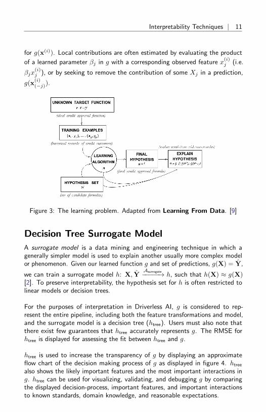
for g(x(i)). Local contributions are often estimated by evaluating the product

of a learned parameter βj in g with a corresponding observed feature x(i)j (i.e.

βjx(i)j ), or by seeking to remove the contribution of some Xj in a prediction,

g(x(i)(−j)).

Figure 3: The learning problem. Adapted from Learning From Data. [9]

Decision Tree Surrogate Model

A surrogate model is a data mining and engineering technique in which agenerally simpler model is used to explain another usually more complex modelor phenomenon. Given our learned function g and set of predictions, g(X) = Y,

we can train a surrogate model h: X, YAsurrogate−−−−−→ h, such that h(X) ≈ g(X)

[2]. To preserve interpretability, the hypothesis set for h is often restricted tolinear models or decision trees.

For the purposes of interpretation in Driverless AI, g is considered to rep-resent the entire pipeline, including both the feature transformations and model,and the surrogate model is a decision tree (htree). Users must also note thatthere exist few guarantees that htree accurately represents g. The RMSE forhtree is displayed for assessing the fit between htree and g.

htree is used to increase the transparency of g by displaying an approximateflow chart of the decision making process of g as displayed in figure 4. htreealso shows the likely important features and the most important interactions ing. htree can be used for visualizing, validating, and debugging g by comparingthe displayed decision-process, important features, and important interactionsto known standards, domain knowledge, and reasonable expectations.


Figure 4: A summarization of a complex model’s decision process as representedby a decision tree surrogate.

Figure 4 displays the decision tree surrogate, htree, for an example probabilityof default model, g, created with Driverless AI using the UCI repository creditcard default data [10]. The PAY 0 feature is likely the most important featurein g due to its place in the initial split in htree and its second occurrence onthe third level of htree. First level interactions between PAY 0 and PAY 2and between PAY 0 and PAY 5 are visible along with several second levelinteractions. Following the decision path to the lowest probability leaf node inhtree (figure 4 lower left) shows that customers who pay their first (PAY 0) andsecond (PAY 2) month bills on time are the least likely to default accordingto htree. The thickness of the edges in this path indicate that this is a verycommon decision path through htree. Following the decision path to the highestprobability leaf node in htree (figure 4 second from right) shows that customerswho are late on their first (PAY 0) and fifth (PAY 5) month bills and whopay less than 16520 in their sixth payment (PAY AMT6) are the most likely todefault according to htree. The thinness of the edges in this path indicate thatthis is a relatively rare decision path through htree. When an observation ofdata is selected using the K -LIME plot, discussed in section 2.3, htree can alsoprovide a degree of local interpretability. When a single observation, x(i), isselected, its path through htree is highlighted. The path of x(i) through htreecan be helpful when analyzing the logic or validity of g(x(i)).

MLI Taxonomy: Decision Tree Surrogate Models

• Scope of Interpretability. (1) Generally, decision tree surrogates provideglobal interpretability. (2) The attributes of a decision tree are usedto explain global attributes of a complex Driverless AI model such asimportant features, interactions, and decision processes.

• Appropriate Response Function Complexity. Decision tree surrogatemodels can create explanations for models of nearly any complexity.


• Understanding and Trust. (1) Decision tree surrogate models fosterunderstanding and transparency because they provide insight into theinternal mechanisms of complex models. (2) They enhance trust, ac-countability, and fairness when their important features, interactions, anddecision paths are in line with human domain knowledge and reasonableexpectations.

• Application Domain. Decision tree surrogate models are model agnostic.

K-LIME

K -LIME is a variant of the LIME technique proposed by Ribeiro et al [8].With K -LIME, local generalized linear model (GLM) surrogates are used toexplain the predictions of complex response functions, and local regions aredefined by K clusters or user-defined segments instead of simulated, perturbedobservation samples. Currently in Driverless AI, local regions are segmentedwith K-means clustering, separating the input training data into K disjointsets: {X0 ∪X1 ∪ . . .XK−1} = X.

For each cluster, a local GLM model hGLM,k is trained. K is chosen such thatpredictions from all the local GLM models would maximize R2. This can besummarized mathematically as follows:

(Xk, g(Xk))AGLM−−−→ hGLM,k,∀k ∈ {0, . . . ,K − 1}

argmaxK

R2(Y, hGLM,k(Xk)),∀k ∈ {0, . . . ,K − 1}

K -LIME also trains one global surrogate GLM hglobal on the entire input trainingdataset and global model predictions g(X). If a given k-th cluster has less than20 members, then hglobal is used as a linear surrogate instead of hGLM,k. Inter-cepts, coefficients, R2 values, accuracy, and predictions from all the surrogateK-LIME models (including the global surrogate) can be used to debug andincrease transparency in g.

In Driverless AI, global K -LIME information is available in the global rankedpredictions plot and the global section of the explanations dialog. The param-eters of hglobal give an indication of overall linear feature importance and theoverall average direction in which an input feature influences g.

Figure 5 depicts a ranked predictions plot of g(X), hglobal(X), and actual targetvalues Y for the example probability of default model introduced in section 2.2.For N input training data observations ordered by index i = {0, . . . , N − 1},let’s sort the global model predictions g(X) from smallest to largest and define


an index ` = {0, . . . , N − 1} for this ordering. The x-axis of the ranked pre-diction plot is `, and the y-axis is the correspond predictions values: g(x(`)),hGLM,k(x(`)) (or hglobal(x

(`))), and y(`).

Figure 5: A ranked predictions plot of a global GLM surrogate model.

The global ranked predictions plot itself can be used as a rough diagnostic tool.In figure 5 it can be seen that g accurately models the original target, givinglow probability predictions when most actual target values are 0 and giving highprobability values when most actual target values are 1. Figure 5 also indicatesthat g behaves nonlinearly as the predictions of the global GLM surrogate,hglobal(x

(`)), are quite far from g(x(`)) in some cases. All displayed behavior ofg is expected in the example use case. However, if this is not the case, usersare encouraged to remove any potentially problematic features from the originaldata and retrain g or to retrain g on the same original features but adjust thesettings in the new Driverless AI experiment to train a more acceptable model.

The coefficient parameters for each hGLM,k can be used to profile a local regionof g, to give an average description of the important features in the local regionand to understand the average direction in which an input feature affects g(x(`)).In Driverless AI, this information is available in the ranked predictions plot foreach cluster as in figure 6 or in the cluster section of the explanations dialog.While coefficient parameter values are useful, reason code values that providethe user with a feature’s approximate local, linear contribution to g(x(`)) canbe generated from K -LIME. Reason codes are powerful tools for accountabilityand fairness because they provide an explanation for each g(x(`)), enablingthe user to understand the approximate magnitude and direction of an inputfeature’s local contribution for g(x(`)). In K -LIME, reason code values arecalculated by determining each coefficient-feature product. Reason code valuesare also written into automatically generated reason codes, available in the localreason code section of the explanations dialog (figure 7). A detailed exampleof calculating reason codes using K -LIME and the credit card default data


introduced in section 2.2 is explained in an upcoming sub-section.

Like all LIME explanations based on GLMs, the local explanations are lin-ear in nature and are offsets from the baseline prediction, or intercept, whichrepresents the average of the hGLM,k model residuals. Of course, linear ap-proximations to complex non-linear response functions will not always createsuitable explanations, and users are urged to check the appropriate rankedpredictions plot, the local GLM R2 in the explanation dialog, and the accuracyof the hGLM,k(x(`)) prediction to understand the validity of the K -LIME reasoncodes. When hGLM,k(x(`)) accuracy for a given point or set of points is quitelow, this can be an indication of extremely nonlinear behavior or the presenceof strong or high-degree interactions g. In cases where hGLM,k is not fitting gwell, nonlinear LOCO feature importance values, discussed in section 2.5, maybe a better explanatory tool for local behavior of g. As K -LIME reason codesrely on the creation of K -means clusters, extremely wide input data or strongcorrelation between input features may also degrade the quality of K -LIMElocal explanations.

K-LIME Reason Codes

For hGLM,k and observation x(i):

g(x(i)) ≈ hGLM,k(x(i)) = β[k]0 +

P∑p=1

β[k]p x(i)p (1)

By disaggregating the K -LIME predictions into individual coefficient-feature

products, β[k]p x

(i)p , the local, linear contribution of the feature can be determined.

This coefficient-feature product is referred to as a reason code value and is usedto create reason codes for each g(x(`)), as displayed in figures 6 and 7.

In this example, reason codes are generated by evaluating and disaggregating thelocal GLM presented in figure 6. The ranked predictions plot for the local GLM(cluster zero), hGLM,0, is highlighted for observation index i = 62 (not rankedordered index `) and displays a K -LIME prediction of 0.817 (i.e. hGLM,0(x(62)) =0.817), a Driverless AI prediction of 0.740 (i.e. g(x(62)) = 0.740), and anactual target value of 1 (i.e. y(62) = 1). The five largest positive and negative

reason code values, β[0]p x

(i)p , are also displayed. Using the displayed reason code

values in figure 6 and the automatically generated reason codes in figure 7and following equation 1, it can be seen that hGLM,0(x(62)) is an acceptableapproximation to the g(x(62)): hGLM,0(x(62)) = 0.817 ≈ g(x(62)) = 0.740.This indicates displayed reason code values are likely to be accurate.


Figure 6: A ranked predictions plot of a local GLM surrogate model withselected observation and reason code values displayed.

Figure 7: Automatically generated reason codes.

A partial disaggregation of hGLM,0 into reason code values can also be derivedfrom the displayed information in figures 6 and 7:

hGLM,0(x(62)) = β[0]0 + β

[0]PAY 0x

(62)PAY 0

+ β[0]PAY 2x

(62)PAY 2 + β

[0]PAY 3x

(62)PAY 3 + βPAY 5x

(62)PAY 5

+ β[0]PAY 6x

(62)PAY 6 + ...+ β

[0]P x

(62)P

(2)

hGLM,0(x(62)) = 0.418 + 0.251

+ 0.056 + 0.041 + 0.037

+ 0.019 + ...+ β[0]P x

(62)P

(3)

where 0.418 is the intercept or baseline of hGLM,0 in figure 7, and the remainingnumeric terms of equation 3 are taken from the reason code values in figure 6.


Other reason codes, whether large enough to be displayed by default or not,follow the same logic.

All of the largest reason code values in the example are positive, meaningthey all contribute to the customer’s high probability of default. The largest

contributor to the customer’s probability of default is β[0]PAY 0x

(62)PAY 0, or in plainer

terms, PAY 0 = 2 months delayed increases the customer’s probabilityof default by approximately 0.25 or by 25%. This is the most important reasoncode in support the g(x(i)) probability for the customer defaulting next month.For this customer, according to K -LIME, the five most important reason codescontributing to their high g(x(i)) probability of default in ranked order are:

• PAY 0 = 2 months delayed





Using the global versus local analysis motif to reason about the example analysisresults thus far, it could be seen as a sign of explanatory stability that severalglobally important features identified by the decision tree surrogate in section2.2 are also appearing as locally important in K -LIME.

MLI Taxonomy: K-LIME

• Scope of Interpretability. K -LIME provides several different scales ofinterpretability: (1) coefficients of the global GLM surrogate provideinformation about global, average trends, (2) coefficients of in-segmentGLM surrogates display average trends in local regions, and (3) whenevaluated for specific in-segment observations, K -LIME provides reasoncodes on a per-observation basis.

• Appropriate Response Function Complexity. (1) K -LIME can createexplanations for machine learning models of high complexity. (2) K -LIME accuracy can decrease when the Driverless AI model becomes toononlinear.

• Understanding and Trust. (1) K -LIME increases transparency by re-vealing important input features and their linear trends. (2) K -LIMEenhances accountability by creating explanations for each observation ina dataset. (3) K -LIME bolsters trust and fairness when the importantfeatures and their linear trends around specific records conform to humandomain knowledge and reasonable expectations.

• Application Domain. K -LIME is model agnostic.


Partial Dependence and Individual Conditional Ex-pectation

One-Dimensional Partial Dependence

For a P -dimensional feature space, we can consider a single feature Xj ∈ Pand its complement set X(−j) (i.e Xj ∪ X(−j) = P). The one-dimensionalpartial dependence of a function g on Xj is the marginal expectation:

PD(Xj , g) = EX(−j)

[g(Xj , X(−j))

](4)

Recall that the marginal expectation over X(−j) sums over the values of X(−j).Now we can explicitly write one-dimensional partial dependence as:

PD(Xj , g) = EX(−j)

[g(Xj , X(−j))

]=

1

N

N−1∑i=0

g(Xj ,x(i)(−j))

(5)

Equation 5 essentially states that the partial dependence of a given feature Xj

is the average of the response function g, setting the given feature Xj = xj

and using all other existing feature vectors of the complement set x(i)(−j) as they

exist in the dataset.

Partial dependence plots show the partial dependence as a function of specificvalues of our feature subset Xj . The plots show how machine-learned responsefunctions change based on the values of an input feature of interest, whiletaking nonlinearity into consideration and averaging out the effects of all otherinput features. Partial dependence plots enable increased transparency in g andenable the ability to validate and debug g by comparing a feature’s averagepredictions across its domain to known standards and reasonable expectations.

Figure 8 displays the one-dimensional partial dependence and ICE (see section2.4.2) for a feature in the example credit card default data Xj = LIMIT BALfor balance limits of xj ∈ {10, 000, 114, 200, 218, 400, ..., 947, 900}. The par-tial dependence (bottom Figure 8) gradually decreases for increasing valuesof LIMIT BAL, indicating that the average predicted probability of defaultdecreases as customer balance limits increase. The grey bands above andbelow the partial dependence curve are the standard deviations of the individualpredictions, g(x(i)), across the domain of Xj . Wide standard deviation bandscan indicate the average behavior of g (i.e., its partial dependence) is nothighly representative of individual g(x(i)), which is often attributable to strong


interactions between Xj and some X(−j). As the displayed curve in figure 8 isaligned with well-known business practices in credit lending, and its standarddeviation bands are relatively narrow, this result should bolster trust in g.

Figure 8: Partial dependence and ICE.

Individual Conditional Expectation

Individual conditional expectation (ICE) plots, a newer and less well-knownadaptation of partial dependence plots, can be used to create more localizedexplanations for a single observation of data using the same basic ideas aspartial dependence plots. ICE is also a type of nonlinear sensitivity analysisin which the model predictions for a single observation are measured while afeature of interest is varied over its domain.

Technically, ICE is a disaggregated partial dependence of the N responses

g(Xj ,x(i)(−j)), i ∈ {1, . . . , N} (for a single feature Xj), instead of averaging the

response across all observations of the training set [3]. An ICE plot for a single

observation x(i) is created by plotting g(Xj = xj,q,x(i)(−j)) versus Xj = xj,q,

(q ∈ {1, 2, . . . }) while fixing x(i)(−j).

ICE plots enable a user to assess the Driverless AI model’s prediction foran individual observation of data, g(x(i)):

1. Is it outside one standard deviation from the average model behaviorrepresented by partial dependence?

2. Is the treatment of a specific observation valid in comparison to averagemodel behavior, known standards, domain knowledge, and reasonableexpectations?


3. How will the observation behave in hypothetical situations where onefeature, Xj , in a selected observation is varied across its domain?

In Figure 8, the selected observation of interest and feature of interest are x(62)

and XLIMIT BAL, respectively. The ICE curve’s values, g(XLIMIT BAL,x(62)(−LIMIT BAL)),

are much larger than PD(XLIMIT BAL, g), clearly outside of the grey standarddeviation regions. This result is parsimonious with previous findings, as thecustomer represented by x(62) was shown to have a high probability of defaultdue to late payments in section 2.3. Figure 8 also indicates that the predictionbehavior for the customer represented by x(62) is somewhat rare in the trainingdata, and that no matter what balance limit the customer is assigned, they willstill be very likely to default according the Driverless AI model.

MLI Taxonomy: Partial Dependence and ICE

• Scope of Interpretability. (1) Partial dependence is a global inter-pretability measure. (2) ICE is a local interpretability measure.

• Appropriate Response Function Complexity. Partial dependence andICE can be used to explain response functions of nearly any complexity.

• Understanding and Trust. (1) Partial dependence and ICE increaseunderstanding and transparency by describing the nonlinear behavior ofcomplex response functions. (2) Partial dependence and ICE enhancetrust, accountability, and fairness by enabling the comparison of describednonlinear behavior to human domain knowledge and reasonable expecta-tions. (3) ICE, as a type of sensitivity analysis, can also engender trustwhen model behavior on simulated data is acceptable.

• Application Domain. Partial dependence and ICE are model-agnostic.

Feature Importance

Feature importance measures the effect that a feature has on the predictionsof a model. Global feature importance measures the overall impact of aninput feature on the Driverless AI model predictions while taking nonlinearityand interactions into consideration. Global feature importance values give anindication of the magnitude of a feature’s contribution to model predictionsfor all observations. Unlike regression parameters, they are often unsigned andtypically not directly related to the numerical predictions of the model. Localfeature importance describes how the combination of the learned model rules orparameters and an individual observation’s attributes affect a model’s predictionfor that observation while taking nonlinearity and interactions into effect.


Figure 9: Global random forest and local LOCO feature importance.

Random Forest Feature Importance

Currently in Driverless AI, a random forest surrogate model hRF consisting ofB decision trees htree,b is trained on the predictions of the Driverless AI model.

hRF(x(i)) =1

B

B∑b=1

htree,b

(x(i); Θb

), (6)

Here Θb is the set of splitting rules for each tree htree,b. As explained in [5],at each split in each tree htree,b, the improvement in the split-criterion is theimportance measure attributed to the splitting feature. The importance measureis accumulated over all trees seperately for each feature. The aggregated featureimportance values are then scaled between 0 and 1, such that the most importantfeature has an importance value of 1.

Figure 9 displays the global and local feature importance values for the creditcard default data, sorted in descending order from the globally most importantfeature to the globally least important feature. Local feature importance valuesare displayed under the global feature importance value for each feature. Infigure 9, PAY 0, PAY 2, LIMIT BAL, PAY 3, and BILL AMT1 are the top5 most important features globally. As expected, this result is well alignedwith the results of the decision tree surrogate model discussed in section 2.2.Taking the results of two interpretability techniques into consideration, it isextremely likely that timing of the customer’s first 3 payments, PAY 0, PAY 2,and PAY 3, are the most important global features for any g(x(i)) prediction.


LOCO Feature Importance

Leave-one-covariate-out (LOCO) provides a mechanism for calculating featureimportance values for any model g on a per-observation basis x(i) by subtractingthe model’s prediction for an observation of data, g(x(i)), from the model’sprediction for that observation of data without an input feature Xj of interest,

g(x(i)(−j))− g(x

(i)) [4]. LOCO is a model-agnostic idea, and g(x(i)(−j)) can be

calculated in various ways. However, in Driverless AI, g(x(i)(−j)) is currently

calculated using a model-specific technique in which the contribution Xj tog(x(i)) is approximated by using random forest surrogate model hRF. Specifically,

the prediction contribution of any rule θ[b]r ∈ Θb containing Xj for tree htree,b is

subtracted from the original prediction htree,b(x(i); Θb

). For the random forest:

g(x(i)(−j)) = hRF(x

(i)(−j)) =

1

B

B∑b=1

htree,b

(x(i); Θb,(−j)

), (7)

where Θb,(−j) is the set of splitting rules for each tree htree,b with the con-tributions of all rules involving feature Xj removed. Although LOCO featureimportance values can be signed quantities, they are scaled between 0 and 1such that the most important feature for an observation of data, x(i), has animportance value of 1 for direct global versus local comparison to random forestfeature importance in Driverless AI.

In figure 9, LOCO local feature importance values are displayed under globalrandom forest feature importance values for each Xj , and the global and localfeature importance for PAY 2 are highlighted for x(62) in the credit card defaultdata. From the nonlinear LOCO perspective, the most important local featuresfor g(x(62)) are PAY 0, PAY 5, PAY 6, PAY 2, and BILL AMT1. Becausethere is good alignment between the linear K -LIME reason codes and LOCOlocal feature importance values, it is extremely likely that PAY 0, PAY 2, PAY 5,and PAY 6 are the most locally important features contributing to g(x(62)).

MLI Taxonomy: Fearture Importance

• Scope of Interpretability. (1) Random forest feature importance is aglobal interpretability measure. (2) LOCO feature importance is a localinterpretability measure.

• Appropriate Response Function Complexity. Both random forest andLOCO feature importance can be used to explain tree-based responsefunctions of nearly any complexity.

• Understanding and Trust. (1) Random forest feature importance in-creases transparency by reporting and ranking influential input features.


(2) LOCO feature importance enhances accountability by creating ex-planations for each model prediction. (3) Both global and local featureimportance enhance trust and fairness when reported values conform tohuman domain knowledge and reasonable expectations.

• Application Domain. (1) Random forest feature importance is a model-specific explanatory technique. (2) LOCO is a model-agnostic concept,but its implementation in Driverless AI is model specific.

Expectations for Consistency Between Explana-tory Techniques

Because machine learning models have intrinsically high variance, it is rec-ommended that users look for explanatory themes that occur across multipleexplanatory techniques and that are parsimonious with reasonable expectationsor human domain knowledge. However, when looking for similarities betweendecision tree surrogates, K -LIME, partial dependence, ICE, sensitivity analysis,and feature importance, note that each technique is providing a different per-spective into a complex, nonlinear, non-monotonic, and even noncontinuousresponse function.

The decision tree surrogate is a global, nonlinear description of the DriverlessAI model behavior. Features that appear in the tree should have a directrelationship with features that appear in the global feature importance plot.For more linear Driverless AI models, features that appear in the decision treesurrogate model may also have large coefficients in the global K -LIME model.

K -LIME explanations are linear, do not consider interactions, and representoffsets from the local GLM intercept. LOCO importance values are nonlinear,do consider interactions, and do not explicitly consider a linear intercept oroffset. K -LIME explanations and LOCO importance values are not expected tohave a direct relationship but should align roughly as both are measures of afeature’s local contribution on a model’s predictions, especially in more linearregions of the Driverless AI model’s learned response function.

ICE has a complex relationship with LOCO feature importance values. Com-paring ICE to LOCO can only be done at the value of the selected featurethat actually appears in the selected observation of the training data. Whencomparing ICE to LOCO, the total value of the prediction for the observation,the value of the feature in the selected observation, and the distance of the ICEvalue from the average prediction for the selected feature at the value in theselected observation must all be considered.

Partial dependence takes into consideration nonlinear, but average, behavior ofthe complex Driverless AI model. Strong interactions between input features

24 | Use Cases

can cause ICE values to diverge from partial dependence values. ICE curvesthat are outside the standard deviation of partial dependence would be expectedto fall into less populated decision paths of the decision tree surrogate; ICEcurves that lie within the standard deviation of partial dependence would beexpected to belong to more common decision paths.

Correcting Unreasonable Models

Once users have gained an approximate understanding of the Driverless AIresponse function using the tools described in sections 2.2 - 2.5, it is crucialto evaluate whether the displayed global and local explanations are reasonable.Explanations should inspire trust and confidence in the Driverless AI model. Ifthis is not the case, users are encouraged to remove potentially problematicfeatures from the original data and retrain the Driverless AI model. Users mayalso retrain the model on the same original features but change the settings inthe Driverless AI experiment to create a more reasonable model.

Use Cases

Use Case: Titanic Survival Model Explanations

We have trained a Driverless AI model to predict survival on the well-knownTitanic dataset. The goal of this use case is to explain and validate themechanisms and predictions of the Driverless AI model using the techniquespresented in sections 2.2 - 2.5.

Data

The Titanic dataset is available from: https://s3.amazonaws.com/h2o-public-test-data/smalldata/gbm test/titanic.csv.

The data consist of passengers on the Titanic. The prediction target is whetheror not a passenger survived (survive). The dataset contains 1,309 passengers,of which 500 survived. Several features were removed from the dataset includingname, boat, body, ticket, and home.dest due to data leakage, as well asambiguities that can hinder interpreting the Driverless AI model. The remaininginput features are summarized in tables 1 and 2.

https://s3.amazonaws.com/h2o-public-test-data/smalldata/gbm_test/titanic.csv

https://s3.amazonaws.com/h2o-public-test-data/smalldata/gbm_test/titanic.csv

Use Cases | 25

Table 1: Summary of numeric input features in the Titanic dataset.

Statistic N Mean St. Dev. Min Max

age 1,309 29.88 14.41 0.17 80sibsp 1,309 0.50 1.04 0 8parch 1,309 0.39 0.87 0 9fare 1,309 33.30 51.76 0 512.33

Table 2: Summary of categorical input features in the Titanic dataset.pclass sex cabin embarked

1 1:323 female:466 :1014 : 22 2:277 male :843 C23 C25 C27 : 6 C:2703 3:709 B57 B59 B63 B66: 5 Q:1234 G6 : 5 S:9145 B96 B98 : 46 C22 C26 : 47 (Other) : 271

Sex, pclass, and age are expected to be globally important in the DriverlessAI model. The summaries show that woman are much more likely to survivethan men (73% vs 19%) and that first class passengers and children have asurvival rate of over 50% compared with the overall survival rate of 38%.

K-LIME

Figure 10: K -LIME plot for the Titanic survival model.

26 | Use Cases

The K -LIME plot in figure 10 shows the Driverless AI model predictions as acontinuous curve starting on the lower left and ending in the upper right. TheK -LIME model predictions are the discontinuous points around the DriverlessAI model predictions. Considering the global explanations in figure 11, we canalso see that the K -LIME predictions generally follow the Driverless AI model’spredictions, and the global K -LIME model explains about 75% of the variabilityin the Driverless AI model predictions, indicating that global explanations areapproximate, but reasonably so.

Figure 11: Global explanations for the Titanic survival model.

Figure 11 presents global explanations for the Driverless AI model. The ex-planations provide a linear understanding of input features and the outcome,survive, in plain English. As expected, they indicate that sex and pclassmake the largest global, linear contributions to the Driverless AI model.

Feature Importance

Figure 12: Feature importance for the Titanic survival model.

Use Cases | 27

The features with the greatest importance values in the Driverless AI modelare sex, cabin, and age as displayed in figure 12. Class is not ranked asa top feature, and instead cabin is assigned a high importance value. cabindenotes the cabin location of the passenger. The first letter of the cabin tellsus the deck level of the passenger. For example, all cabins that start with Acorrespond to cabins in the upper promenade deck. Further data explorationindicates that first class passengers stayed in the top deck cabins, above secondclass passengers in the middle decks, and above third class passengers at thelowest deck levels. This correlation between cabin and pclass may explainwhy cabin is located higher than pclass in the global feature importanceplot, especially if cabin contains similar but more granular information thanpclass.

The feature importance figure matches hypotheses created during data explo-ration to a large extent. Feature importance, however, does not explain therelationship between a feature and the Driverless AI model’s predictions. Thisis where we can examine partial dependence plots.

Partial Dependence Plots

The partial dependence plots show how different values of a feature affectthe average prediction of the Driverless AI model. Figure 13 displays thepartial dependence plot for sex and indicates that predicted survival increasesdramatically for female passengers.

Figure 13: Partial dependence plot for sex for the Titanic survival model.

Figure 14 displays the partial dependence plot for age. The Driverless AI modelpredicts high probabilities for survival for passengers younger than 17. After theage of 17, increases in age do not result in large changes in the Driverless AImodel’s average predictions. This result is in agreement with previous findingsin which children have a higher probability of survival.

28 | Use Cases

Figure 14: Partial dependence plot for age for the Titanic survival model.

Decision Tree Surrogate

In figure 15, the RMSE of 0.164 indicates the decision tree surrogate is ableto approximate the Driverless AI model well. By following the decision pathsdown the decision tree surrogate, we can begin to see details in the DriverlessAI model’s decision processes. For example, it is not totally accurate to assumethat all women will survive. Women in third class who paid a small amount fortheir fare actually have a lower prediction than the overall average survival rate.Likewise, there are some groups of men with high average predictions. Menwith a cabin beginning in A (the top deck of the ship) have an average survivalprediction greater than 75%.

Figure 15: Decision tree surrogate for the Titanic survival model.

Local Explanations

Following the global versus local analysis motif, local contributions to modelpredictions for a single passenger are also analyzed and compared to global

Use Cases | 29

explanations and reasonable expectations. Figure 16 shows the local dashboardafter selecting a single passenger in the K -LIME plot. For this example usecase, a female with a first class ticket is selected.

Figure 16: Local interpretability dashboard for a single female passenger.

In figure 16, the path of the selected individual through the far right decisionpath in the decision tree surrogate model is highlighted. This selected passengerfalls into the leaf node with the greatest average model prediction for survival,which is nicely aligned with the Driverless AI model’s predicted probability forsurvival of 0.89.

Figure 17: Local feature importance for a single female passenger.

When investigating observations locally, the feature importance has two barsper feature. The upper bar represents the global feature importance and thelower bar represents the local feature importance. In figure 17, the two featuressex and cabin are the most important features both globally and locally forthe selected individual.

30 | Use Cases

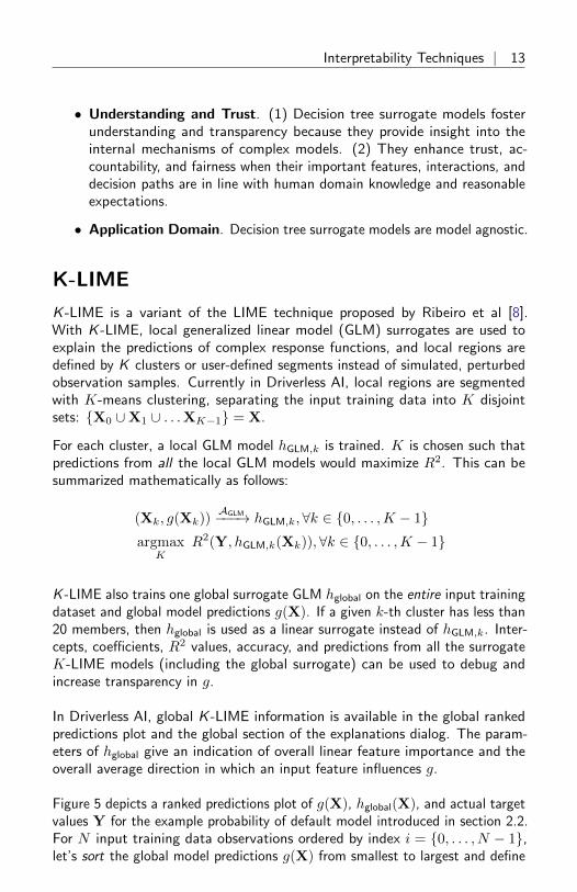
Figure 18: Partial dependence and ICE for a single female passenger.

The local dashboard also overlays ICE curves onto partial dependence plots.In figure 18, the lower points for partial dependence remain unchanged fromfigure 13 and show the average model prediction by sex. The upper pointsindicate how the selected passenger’s prediction would change if their valuefor sex changed, and figure 18 indicates that her prediction for survival woulddecrease dramatically if her value for sex changed to male. Figure 18 alsoshows that the selected passenger is assigned a higher-than-average survivalrate regardless of sex. This result is most likely due to the selected individualbeing a first class passenger.

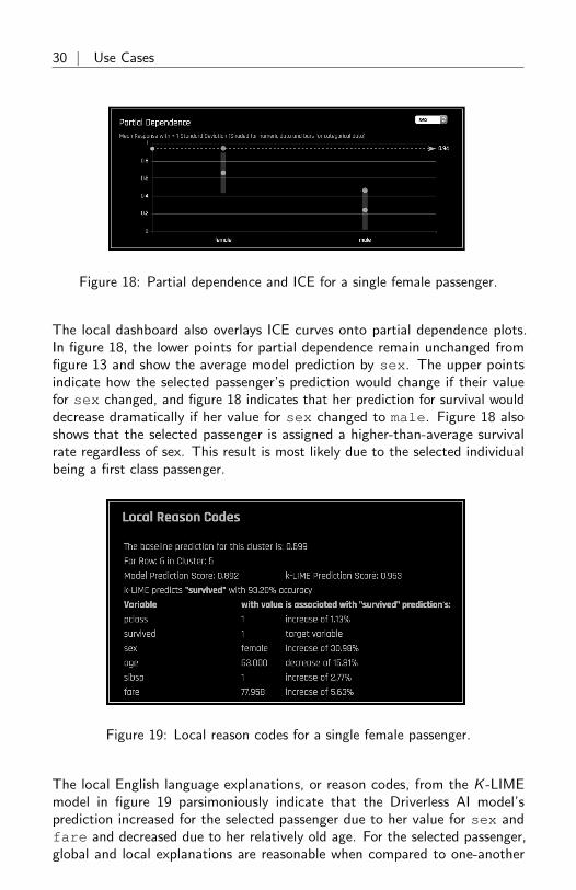
Figure 19: Local reason codes for a single female passenger.

The local English language explanations, or reason codes, from the K -LIMEmodel in figure 19 parsimoniously indicate that the Driverless AI model’sprediction increased for the selected passenger due to her value for sex andfare and decreased due to her relatively old age. For the selected passenger,global and local explanations are reasonable when compared to one-another

Use Cases | 31

and to logical expectations. In practice, explanations for several different typesof passengers, and especially for outliers and other anomalous observations,should be investigated and analyzed to enhance understanding and trust in theDriverless AI model.

Use Case: King County Housing Model Explana-tions

We have trained a Driverless AI model to predict housing prices in King County,Washington. The goal of this use case is to explain and validate the mechanismsand predictions of the trained Driverless AI model using the techniques presentedin sections 2.2 - 2.5.

Data

The housing prices dataset is available from: https://www.kaggle.com/harlfoxem/housesalesprediction.

This dataset contains house sale prices for King County, Washington, whichincludes Seattle. It includes homes sold between May 2014 and May 2015.The prediction target is housing price, price. Several features were removedfrom the analysis including ID, date, latitude, longitude, zipcode,and several other ambiguous or multicollinear features that could hinder inter-pretability. The remaining input features are summarized in tables 3 and 4. Theoutcome price is right-skewed, requiring a log transform before training aDriverless AI model.

Table 3: Summary of numeric input features in the housing prices dataset.

Statistic N Mean St. Dev. Min Max

price 21,613 540,088.100 367,127.200 75,000 7,700,000sqft living 21,613 2,079.900 918.441 290 13,540sqft lot 21,613 15,106.970 41,420.510 520 1,651,359sqft above 21,613 1,788.391 828.091 290 9,410sqft basement 21,613 291.509 442.575 0 4,820yr built 21,613 1,971.005 29.373 1,900 2,015yr renovated 21,613 84.402 401.679 0 2,015

https://www.kaggle.com/harlfoxem/housesalesprediction

https://www.kaggle.com/harlfoxem/housesalesprediction

32 | Use Cases

Table 4: Summary of categorical input features in the housing prices dataset.bathrooms bedrooms floors waterfront view condition

1 2.5 :5380 3 :9824 1.0:10680 0:21450 0:19489 1: 302 1.0 :3852 4 :6882 1.5: 1910 1: 163 1: 332 2: 1723 1.75 :3048 2 :2760 2.0: 8241 2: 963 3:140314 2.25 :2047 5 :1601 2.5: 161 3: 510 4: 56795 2.0 :1930 6 : 272 3.0: 613 4: 319 5: 17016 1.5 :1446 1 : 199 3.5: 87 (Other):3910 (Other): 75

Living square footage, sqft living, is linearly associated with increases inprice with a correlation coefficient of greater than 0.6. There is also a linearlyincreasing trend between the number of bathrooms and the home price.The more bathrooms, the higher the home price. Hence, inputs relatedto square footage and the number of bathrooms are expected to be globallyimportant in the Driverless AI model.

K-LIME

Figure 20: K -LIME plot for the King County home prices model.

The K -LIME plot in figure 20 shows the Driverless AI model predictions as acontinuous curve starting at the middle left and ending in the upper right. TheK -LIME model predictions are the discontinuous points around the DriverlessAI model predictions. In figure 20, K -LIME accurately traces the original target,and according to figure 21, K -LIME explains 92 percent of the variability inthe Driverless AI model predictions. The close fit of K -LIME to the DriverlessAI model indicates that the global explanations in figure 21 very likely to beinsightful and trustworthy.

Use Cases | 33

Figure 21: Global explantions for the King County home prices model.

The explanations provide a linear understanding of input features and theoutcome, price. (Note, the K -LIME explanations are in the log() space forprice.) For example:

When bathrooms increase by 1 unit, this is associated withprice K -LIME predictions increase of 0.076

This particular explanation falls in line with findings from data exploration insection 3.2.1 and with reasonable expectations. The more bathrooms a househas, the higher the price.

Another interesting global explanation relates to the year when a house wasbuilt.

When yr built increases by 1 unit, this is associated with priceK -LIME predictions decrease of 0.004

This explanation indicates newer homes will have a lower price than olderhomes. We will explore this, perhaps counterintuitive, finding further with apartial dependence plot in section 3.2.4 and a decision tree surrogate model insection 3.2.5.

34 | Use Cases

Feature Importance

Figure 22: Feature Importance for the King County home prices model.

According to figure 22, the features with the largest global importance inthe Driverless AI model are sqft living, sqft above, yr built, andbathrooms. The high importance of sqft living (total square footage ofthe home), sqft above (total square footage minus square footage of thebasement), and bathrooms follow trends observed during data explorationand are parsimonious with reasonable expectations. yr built is also playing alarge role in the predictions for price, beating out bathrooms just slightly.

Partial Dependence Plots

Partial dependence plots show how different values of a feature affect theaverage prediction for price in the Driverless AI model. Figure 23 indicatesthat as sqft living increases, the average prediction of the Driverless AImodel also increases.

Figure 23: Partial dependence plot of sqft living for the King Countyhome prices model.

In figure 24, the partial dependence for bathrooms can be seen to increaseslightly as the total number of bathrooms increases. Figures 23 and 24 arealigned with findings from data exploration and reasonable expectations.

Use Cases | 35

Figure 24: Partial dependence plot of bathrooms for the King County homeprices model.

Figure 25 displays the partial dependence for yr built, where Driverless AImodel predictions for price decrease as the age of the house decreases. Figure25 confirms the global K -LIME explanation for yr built discussed in section3.2.2. A relationship of this nature could indicate something unique about KingCounty, Washington, but requires domain knowledge to decide whether thefinding is valid or calls the Driverless AI model’s behavior into question.

Figure 25: Partial dependence plot of yr built for the King County homeprices model.

Decision Tree Surrogate

Figure 26: Decision tree surrogate for the King County home prices model.

36 | Use Cases

In figure 26, the RMSE of 0.181 indicates the decision tree surrogate is ableto approximate the Driverless AI model well. By following the decision pathsdown the decision tree surrogate, we can begin to see details in the DriverlessAI model’s decision processes. sqft living is found in the first split and inseveral other splits of the decision tree surrogate, signifying its overall importancein the Driverless AI model and in agreement with several previous findings.

Moving down the left side of the decision tree surrogate, yr built interactswith sqft living. If sqft living is greater than or equal to 1,526 squarefeet and the home was built before 1944, then the price is predicted to belog(13.214), which is about $547,983, but if the home was built after 1944,then the price is predicted to be log(12.946), which is about $419,156.This interaction, which is clearly expressed in the decision tree surrogate model,provides more insight into why older homes are predicted to cost more asdiscussed in sections 3.2.2 and 3.2.4.

Local Explanations

Following the global versus local analysis motif, local contributions to modelpredictions for a single home are also analyzed and compared to global explana-tions and reasonable expectations. Figure 27 shows the local dashboard afterselecting a single home in the K -LIME plot. For this example use case, theleast expensive home is selected.

Figure 27: Local interpretability dashboard for the least expensive home.

Figure 28 shows the feature importance plot with two bars per feature. The topbar represents the global feature importance and the bottom bar represents thelocal feature importance. Locally for the least expensive home, bathroomsis the most important feature followed by sqft living, sqft above, and

Use Cases | 37

yr built. What might cause this difference between global and local featureimportance values? It turns out the least expensive home has zero bathrooms!

Figure 28: Local feature importance for the least expensive home.

The local dashboard also overlays ICE onto the partial dependence plot, asseen in figure 29. The upper partial dependence curve in figure 29 remainsunchanged from figure 24 and shows the average Driverless AI model predictionby the number of bathrooms. The lower ICE curve in figure 29 indicates howthe least expensive home’s price prediction would change if its number ofbathrooms changed, following the global trend of more bathrooms leading tohigher predictions for price.

Figure 29: Partial dependence and ICE for the least expensive home.

The local English language explanations, i.e. reason codes, from K -LIME infigure 30 show that the Driverless AI model’s prediction increased for this homedue to its relatively high sqft living and decreased due to its relativelyrecent yr built, which is aligned with global explanations. Note that thenumber of bathrooms is not considered in K -LIME reason codes becausethis home does not have any bathrooms. Since this home’s local value forbathrooms is zero, bathrooms cannot contribute to the K -LIME model.

38 | Acknowledgements

Figure 30: Reason codes for the least expensive home.

Continuing with the global versus local analysis, explanations for the most expen-sive home are considered briefly. In figure 31, the two features sqft livingand sqft above are the most important features locally along with bathroomsand yr built. The data indicate the most expensive home has eight bathrooms,12050 square feet of total square footage in which 8570 is allocated for livingspace (not including the basement), and the home was built in 1910. Followingglobal explanations and reasonable expectations, this most expensive home hascharacteristics that justify it’s high prediction for price.

Figure 31: Local feature importance for the most expensive home.

For the selected homes, global and local explanations are reasonable when com-pared to one-another and to logical expectations. In practice, explanations forseveral different types of homes, and especially for outliers and other anomalousobservations, should be investigated and analyzed to enhance understandingand trust in the Driverless AI model.

AcknowledgementsThe authors would like to acknowledge the following individuals for their invalu-able contributions to the software described in this booklet: Leland Wilkinson,Mark Chan, and Michal Kurka.

References | 39

References1. Patrick Hall, Wen Phan, and Sri Satish Ambati. Ideas on interpreting

machine learning. O’Reilly Ideas, 2017. URL https://www.oreilly.com/ideas/ideas-on-interpreting-machine-learning

2. Mark W. Craven and Jude W. Shavlik. Extracting tree-structured repre-sentations of trained networks. Advances in Neural Information Process-ing Systems, 1996. URL http://papers.nips.cc/paper/1152-extracting-tree-structured-representations-of-trained-networks.pdf

3. Alex Goldstein, Adam Kapelner, Justin Bleich, and Emil Pitkin. Peekinginside the black box: Visualizing statistical learning with plots of indi-vidual conditional expectation. Journal of Computational and GraphicalStatistics, 24(1), 2015

4. Jing Lei, Max G’Sell, Alessandro Rinaldo, Ryan J. Tibshirani, and LarryWasserman. Distribution-free predictive inference for regression. Journalof the American Statistical Association just-accepted, 2017. URL http://www.stat.cmu.edu/˜ryantibs/papers/conformal.pdf

5. Jerome Friedman, Trevor Hastie, and Robert Tibshirani. The Elementsof Statistical Learning. Springer, New York, 2001. URL https://web.stanford.edu/˜hastie/ElemStatLearn/printings/ESLII print12.pdf

6. Leo Breiman. Statistical modeling: The two cultures (with commentsand a rejoinder by the author). Statistical Science, 16(3), 2001. URLhttps://projecteuclid.org/euclid.ss/1009213726

7. Finale Doshi-Velez and Been Kim. Towards a rigorous science of inter-pretable machine learning. arXiV preprint, 2017

8. Marco Tulio Ribeiro, Sameer Singh, and Carlos Guestrin. Why should Itrust you?: Explaining the predictions of any classifier. In Proceedings ofthe 22nd ACM SIGKDD International Conference on Knowledge Discoveryand Data Mining, pages 1135–1144. ACM, 2016. URL http://www.kdd.org/kdd2016/papers/files/rfp0573-ribeiroA.pdf

9. Yaser S. Abu-Mostafa, Malik Magdon-Ismail, and Hsuan-Tien Lin. Learn-ing from Data. AMLBook, New York, 2012. URL https://work.caltech.edu/textbook.html

10. M. Lichman. UCI machine learning repository, 2013. URL http://archive.ics.uci.edu/ml

https://www.oreilly.com/ideas/ideas-on-interpreting-machine-learning

https://www.oreilly.com/ideas/ideas-on-interpreting-machine-learning

http://papers.nips.cc/paper/1152-extracting-tree-structured-representations-of-trained-networks.pdf



http://www.stat.cmu.edu/~ryantibs/papers/conformal.pdf

http://www.stat.cmu.edu/~ryantibs/papers/conformal.pdf

https://web.stanford.edu/~hastie/ElemStatLearn/printings/ESLII_print12.pdf



https://projecteuclid.org/euclid.ss/1009213726

http://www.kdd.org/kdd2016/papers/files/rfp0573-ribeiroA.pdf

http://www.kdd.org/kdd2016/papers/files/rfp0573-ribeiroA.pdf

https://work.caltech.edu/textbook.html

https://work.caltech.edu/textbook.html

http://archive.ics.uci.edu/ml

http://archive.ics.uci.edu/ml

40 | Authors

AuthorsPatrick Hall

Patrick Hall is senior director for data science products at H2O.ai where hefocuses mainly on model interpretability. Patrick is also currently an adjunctprofessor in the Department of Decision Sciences at George Washington Univer-sity, where he teaches graduate classes in data mining and machine learning.Prior to joining H2O.ai, Patrick held global customer facing roles and researchand development roles at SAS Institute.

Follow him on Twitter: @jpatrickhall

Navdeep Gill

Navdeep is a software engineer and data scientist at H2O.ai. He graduatedfrom California State University, East Bay with a M.S. degree in ComputationalStatistics, B.S. in Statistics, and a B.A. in Psychology (minor in Mathemat-ics). During his education he gained interests in machine learning, time seriesanalysis, statistical computing, data mining, and data visualization. Previous toH2O.ai, Navdeep worked at Cisco Systems, Inc. focusing on data science andsoftware development, and before stepping into industry he worked in variousNeuroscience labs as a researcher and analyst.

Follow him on Twitter: @Navdeep Gill

Megan Kurka

Megan is a customer data scientist at H2O.ai. Prior to working at H2O.ai,she worked as a data scientist building products driven by machine learning forB2B customers. Megan has experience working with customers across multipleindustries, identifying common problems, and designing robust and automatedsolutions.

Wen Phan

Wen Phan is director of customer engineering and data science at H2O.ai.Wen works with customers and organizations to architect systems, smarterapplications, and data products to make better decisions, achieve positiveoutcomes, and transform the way they do business. Wen holds a B.S. inelectrical engineering and M.S. in analytics and decision sciences.

Follow him on Twitter: @wenphan

machine learning interpretability with h2o...

Documents