machine learning for the prediction of professional tennis ... · machine learning for the...
TRANSCRIPT

Imperial College London
MEng Computing – Final year project
Machine Learning for the Prediction ofProfessional Tennis Matches
Author:Michal Sipko
Supervisor:Dr. William Knottenbelt
June 15, 2015


Abstract
Extensive research has been conducted into the modelling of professional tennis matches. Most currentapproaches take advantage of the hierarchical structure of the tennis scoring system to define stochasticmodels, based on Markov chains. These models use only the probability of each of the players winninga point on their serve to compute their respective probabilities of winning the match. Consequently,a variety of factors that contribute to the outcome of a match are ignored. We propose a supervisedmachine learning approach that uses historical player performance across a wide variety of statisticsto predict match outcomes. We define a novel method of extracting 22 features from raw historicaldata, including abstract features, such as player fatigue and injury. Using the resulting dataset, wedevelop and optimise models based on two machine learning algorithms: logistic regression and artificialneural networks. When evaluated on a test set of 6315 ATP matches played in the years 2013-2014, ourmodels outperform Knottenbelt’s Common-Opponent model, the current state-of-the-art in stochasticmodelling. Our neural network generates a return on investment of 4.35% when in competition with thebetting market, an improvement of about 75%. We believe that the use of machine learning will lead toinnovation in the field of tennis modelling.

Acknowledgements
I would like to express my gratitude to Dr William Knottenbelt, for his valuable and constructivesuggestions throughout the project. His enthusiasm for tennis modelling is unmatched.
Special thanks should go to the Stratagem team, for granting access to their dataset and for theirwillingness to discuss the practical aspects of a tennis betting system.

Contents
1 Introduction 1
2 Background 32.1 The Game of Tennis . . . . . . . . . . . . . . . . . . . . . . . . . . . . . . . . . . . . . . . 32.2 The Tennis Dataset . . . . . . . . . . . . . . . . . . . . . . . . . . . . . . . . . . . . . . . . 32.3 Tennis Betting . . . . . . . . . . . . . . . . . . . . . . . . . . . . . . . . . . . . . . . . . . 4
2.3.1 Betting Odds and Implied Probability . . . . . . . . . . . . . . . . . . . . . . . . . 52.3.2 Betting Strategies . . . . . . . . . . . . . . . . . . . . . . . . . . . . . . . . . . . . 5
2.4 Statistical Models . . . . . . . . . . . . . . . . . . . . . . . . . . . . . . . . . . . . . . . . . 62.4.1 Markov Models . . . . . . . . . . . . . . . . . . . . . . . . . . . . . . . . . . . . . . 62.4.2 Hierarchical Expressions . . . . . . . . . . . . . . . . . . . . . . . . . . . . . . . . . 62.4.3 Estimating Serve Winning Probabilities . . . . . . . . . . . . . . . . . . . . . . . . 82.4.4 Current State-of-the-Art . . . . . . . . . . . . . . . . . . . . . . . . . . . . . . . . . 8
2.5 Machine Learning Models . . . . . . . . . . . . . . . . . . . . . . . . . . . . . . . . . . . . 92.5.1 Machine Learning in Tennis . . . . . . . . . . . . . . . . . . . . . . . . . . . . . . . 92.5.2 Logistic Regression . . . . . . . . . . . . . . . . . . . . . . . . . . . . . . . . . . . . 92.5.3 Artificial Neural Networks . . . . . . . . . . . . . . . . . . . . . . . . . . . . . . . . 112.5.4 Support Vector Machines . . . . . . . . . . . . . . . . . . . . . . . . . . . . . . . . 122.5.5 Machine Learning Challenges . . . . . . . . . . . . . . . . . . . . . . . . . . . . . . 12
3 Feature Extraction 133.1 Tennis Match Representation . . . . . . . . . . . . . . . . . . . . . . . . . . . . . . . . . . 13
3.1.1 Match Outcome Representation . . . . . . . . . . . . . . . . . . . . . . . . . . . . . 133.1.2 Symmetric Match Feature Representation . . . . . . . . . . . . . . . . . . . . . . . 13
3.2 Historical Averaging . . . . . . . . . . . . . . . . . . . . . . . . . . . . . . . . . . . . . . . 143.2.1 Common Opponents . . . . . . . . . . . . . . . . . . . . . . . . . . . . . . . . . . . 143.2.2 Time Discounting . . . . . . . . . . . . . . . . . . . . . . . . . . . . . . . . . . . . 153.2.3 Surface Weighting . . . . . . . . . . . . . . . . . . . . . . . . . . . . . . . . . . . . 16
3.3 Uncertainty . . . . . . . . . . . . . . . . . . . . . . . . . . . . . . . . . . . . . . . . . . . . 183.3.1 Uncertainty For Simple Averaging . . . . . . . . . . . . . . . . . . . . . . . . . . . 183.3.2 Uncertainty For Common Opponents . . . . . . . . . . . . . . . . . . . . . . . . . 18
3.4 New Feature Construction . . . . . . . . . . . . . . . . . . . . . . . . . . . . . . . . . . . . 193.4.1 Combining Statistics . . . . . . . . . . . . . . . . . . . . . . . . . . . . . . . . . . . 193.4.2 Modelling Fatigue . . . . . . . . . . . . . . . . . . . . . . . . . . . . . . . . . . . . 203.4.3 Modelling Injury . . . . . . . . . . . . . . . . . . . . . . . . . . . . . . . . . . . . . 213.4.4 Head-to-head Balance . . . . . . . . . . . . . . . . . . . . . . . . . . . . . . . . . . 21
3.5 Data Preparation . . . . . . . . . . . . . . . . . . . . . . . . . . . . . . . . . . . . . . . . . 213.5.1 Data Cleansing . . . . . . . . . . . . . . . . . . . . . . . . . . . . . . . . . . . . . . 213.5.2 Feature Scaling . . . . . . . . . . . . . . . . . . . . . . . . . . . . . . . . . . . . . . 23
3.6 Summary of Features . . . . . . . . . . . . . . . . . . . . . . . . . . . . . . . . . . . . . . . 25
4 Logistic Regression Model 264.1 Dataset Division . . . . . . . . . . . . . . . . . . . . . . . . . . . . . . . . . . . . . . . . . 264.2 Evaluation Metrics . . . . . . . . . . . . . . . . . . . . . . . . . . . . . . . . . . . . . . . . 274.3 Model Symmetry . . . . . . . . . . . . . . . . . . . . . . . . . . . . . . . . . . . . . . . . . 274.4 Feature Selection . . . . . . . . . . . . . . . . . . . . . . . . . . . . . . . . . . . . . . . . . 28
i

4.4.1 Ignoring Rank Information . . . . . . . . . . . . . . . . . . . . . . . . . . . . . . . 284.4.2 Feature Selection Algorithms . . . . . . . . . . . . . . . . . . . . . . . . . . . . . . 284.4.3 Results . . . . . . . . . . . . . . . . . . . . . . . . . . . . . . . . . . . . . . . . . . 30
4.5 Hyperparameter Optimisation . . . . . . . . . . . . . . . . . . . . . . . . . . . . . . . . . . 324.5.1 Optimisation Approach . . . . . . . . . . . . . . . . . . . . . . . . . . . . . . . . . 324.5.2 Noise Removal . . . . . . . . . . . . . . . . . . . . . . . . . . . . . . . . . . . . . . 334.5.3 Time Discount Factor . . . . . . . . . . . . . . . . . . . . . . . . . . . . . . . . . . 334.5.4 Regularisation Parameter . . . . . . . . . . . . . . . . . . . . . . . . . . . . . . . . 34
5 Higher Order Models 355.1 Bias and Variance . . . . . . . . . . . . . . . . . . . . . . . . . . . . . . . . . . . . . . . . 355.2 Logistic Regression with Interaction Features . . . . . . . . . . . . . . . . . . . . . . . . . 36
5.2.1 Constuction of Interaction Features . . . . . . . . . . . . . . . . . . . . . . . . . . . 365.2.2 Model Optimisation . . . . . . . . . . . . . . . . . . . . . . . . . . . . . . . . . . . 36
5.3 Artificial Neural Network . . . . . . . . . . . . . . . . . . . . . . . . . . . . . . . . . . . . 375.3.1 Network structure . . . . . . . . . . . . . . . . . . . . . . . . . . . . . . . . . . . . 385.3.2 Model optimisation . . . . . . . . . . . . . . . . . . . . . . . . . . . . . . . . . . . . 39
6 Implementation Overview 446.1 Data Flow . . . . . . . . . . . . . . . . . . . . . . . . . . . . . . . . . . . . . . . . . . . . . 446.2 Technologies . . . . . . . . . . . . . . . . . . . . . . . . . . . . . . . . . . . . . . . . . . . . 446.3 Efficiency . . . . . . . . . . . . . . . . . . . . . . . . . . . . . . . . . . . . . . . . . . . . . 45
7 Evaluation 467.1 Evaluation Method . . . . . . . . . . . . . . . . . . . . . . . . . . . . . . . . . . . . . . . . 467.2 Results . . . . . . . . . . . . . . . . . . . . . . . . . . . . . . . . . . . . . . . . . . . . . . . 46
7.2.1 ROI and Logistic Loss . . . . . . . . . . . . . . . . . . . . . . . . . . . . . . . . . . 467.2.2 Betting Volume . . . . . . . . . . . . . . . . . . . . . . . . . . . . . . . . . . . . . . 487.2.3 Simulation . . . . . . . . . . . . . . . . . . . . . . . . . . . . . . . . . . . . . . . . 49
7.3 Tennis Insights . . . . . . . . . . . . . . . . . . . . . . . . . . . . . . . . . . . . . . . . . . 497.3.1 Relative Importance of Different Historical Matches . . . . . . . . . . . . . . . . . 497.3.2 Relative Importance of Different Features . . . . . . . . . . . . . . . . . . . . . . . 50
7.4 Limitations . . . . . . . . . . . . . . . . . . . . . . . . . . . . . . . . . . . . . . . . . . . . 517.4.1 Black Box Models . . . . . . . . . . . . . . . . . . . . . . . . . . . . . . . . . . . . 517.4.2 In-play Prediction . . . . . . . . . . . . . . . . . . . . . . . . . . . . . . . . . . . . 517.4.3 Data Collection . . . . . . . . . . . . . . . . . . . . . . . . . . . . . . . . . . . . . . 51
8 Conclusion 528.1 Innovation . . . . . . . . . . . . . . . . . . . . . . . . . . . . . . . . . . . . . . . . . . . . . 528.2 Future Work . . . . . . . . . . . . . . . . . . . . . . . . . . . . . . . . . . . . . . . . . . . 53
8.2.1 Additional Features . . . . . . . . . . . . . . . . . . . . . . . . . . . . . . . . . . . 538.2.2 Women’s Tennis . . . . . . . . . . . . . . . . . . . . . . . . . . . . . . . . . . . . . 538.2.3 Other ML Algorithms . . . . . . . . . . . . . . . . . . . . . . . . . . . . . . . . . . 538.2.4 Set-by-Set Analysis . . . . . . . . . . . . . . . . . . . . . . . . . . . . . . . . . . . . 538.2.5 Hybrid Model . . . . . . . . . . . . . . . . . . . . . . . . . . . . . . . . . . . . . . . 53
Appendices 57
A Additional Figures 57
B Model Parameter Summary 59
ii

Chapter 1
Introduction
Tennis is undoubtedly among the world’s most popular sports. The Association of Tennis Professionals(ATP) features over 60 professional tennis tournaments in 30 countries every year, drawing immensenumbers of spectators. Andy Murray’s historic defeat of Novak Djokovic in the 2013 Wimbledon final wasthe most watched television broadcast of the year in Great Britain, with an audience of 17.3 million. Thegrowth of the popularity of the sport, paired with the expansion of the online sports betting market, hasled to a large increase in tennis betting volume in recent years. The same Murray-Dojokovic Wimbledonfinal saw £48 million traded on Betfair, the world’s largest betting exchange. The potential profit, aswell as academic interest, has fuelled the search for accurate tennis match prediction algorithms.
The scoring system in tennis has a hierarchical structure, with a match being composed of sets, whichin turn are composed of games, which are composed of individual points. Most current state-of-the-art approaches to tennis prediction take advantage of this structure to define hierarchical expressionsfor the probability of a player winning the match. By assuming that points are independently andidentically distributed (iid)1, the expressions only need the probabilities of the two players winning apoint on their serve. From this basic statistic, easily calculated from historical data available online, wecan deduce the probability of a player winning a game, then a set, and finally the match. Barnett [1]and O’Malley [18] both defined such hierarchical models, and Knottenbelt [13] refined the models tocalculate the probabilties of winning a point on serve using only matches with the common opponentsof the players, instead of all past opponents. This reduces the bias resulting from the players havinghistorically had different average opponents. Madurska [16] further extended the Common-Opponentmodel to use different probabilities of winning on serve for different sets, challenging the iid assumptionand allowing the model to reflect the way a player’s performance varies over the course of the match.Knottenbelt’s Common-Opponent model and Madurska’s Set-By-Set model are the current state-of-the-art, claiming a return on investment of 6.8% and 19.6%, respectively, when put into competition withthe betting market on matches in the 2011 WTA Grand Slams.
While elegant, this mathematical approach is not perfect. By representing the quality of players usingonly a single value (service points won), the method is unable to act upon the more subtle factors thatcontribute to the outcome of a match. For example, a player’s susceptibility to a particular playingstrategy (e.g., attacking the net), the time since their last injury, or accumulated fatigue from previousmatches would only indirectly affect match prediction. Furthermore, the characteristics of the match itself(location, weather conditions, etc.) would have no effect on the prediction. Considering the availabilityof an immense amount of diverse historical tennis data, an alternative approach to tennis predictioncould be based on machine learning. The features of players and the features of the match, paired withthe match result, could form a set of labelled training examples. A supervised ML algorithm could usethese examples to infer a function for predicting the results of new matches.
Despite machine learning being a natural candidate for the tennis match prediction problem, the ap-proach seems to have had little attention in comparison with the stochastic hierarchical approaches. Mostpast attempts made use of logistic regression. For example, Clarke and Dyte [6] fit a logistic regressionmodel to the difference in the ATP rating points of the two players for predicting the outcome of a set. A
1Klaasen and Magnus [12] show that points are neither independent nor identically distributed. However, they find thatdeviations from iid are small, and using this assumption often provides good approximations.
1

Machine Learning for the Prediction of Professional Tennis Matches Michal Sipko
simulation then was run to predict the result of several men’s tournaments in 1998 and 1999, producingreasonable results. Ma, Liu and Tan [15] used logistic regression with 16 variables related to character-istics of the players and the match. Investigating a different ML algorithm, Somboonphokkaphan [22]trained an artificial neural network (ANN) using the match surface and several features of both players(winning percentages on first serve, second serve, return, break points, etc.) as training parameters. Theauthors claim an accuracy of about 75% in predicting the matches in the Grand Slam tournaments in2007 and 2008.
The goal of the project is to investigate the applicability of machine learning methods to the prediction ofprofessional tennis matches. We begin by developing an approach for extracting a set of relevant featuresfrom raw historical data (Chapter 3). Next, we train a logistic regression model on the constructed dataset(Chapter 4). Seeking further improvement, we train two higher-order models (logistic regression withinteraction features and an artificial neural network) in Chapter 5. We then evaluate the performanceof the models on an independent dataset of 6135 ATP matches played during the years 2013-2014, usingthree different betting strategies (Chapter 7). We find that our most profitable machine learning modelgenerates a 4.35% return on investment, an improvement of approximately 75% over the current state-of-the-art stochastic models. This shows that a machine learning approach is is well worth pursuing. Wepropose some extensions to our work in Chapter 8.
2

Chapter 2
Background
2.1 The Game of Tennis
Tennis is a racquet sport that can be played either against a single opponent (singles) or betweentwo teams of two players (doubles). For simplicity, we will focus only on modelling singles tennismatches.
At any point in a match, one of the players is designated to be the server, and the other is the receiver.The players stand on opposite sides of the tennis court, a rectangular area with a net stretched across itswidth. Various court surfaces are used in different tournaments, including clay, grass, or hard. After alegal service by the server (for which they have two attempts), the players alternate hitting the ball, untileventually one wins the rally, earning a point. (We omit the full details of the tennis rules for brevity,the official rules are published online by the International Tennis Federation1).
A game consists of a sequence of points with the same player serving. The first player to win at least fourpoints and at least two more than the opponent wins the game. The points are counted in an unsual way,in the sequence 0, 15, 30, 40. If the score reaches 40-40, this is called a deuce. Whichever player winsthe next point has the advantage, because winning another point will result in them winning the game.After each game, the players alternate at serving. The first player to win at least six games and at leasttwo more than the opponent wins the set. However, if the set score reaches 6-6, in most tournaments,a tiebreaker is played, a special game in which the first player to have won at least seven points and atleast two more than the opponent wins the set. A match is won when a player wins the majority of aspecified number of sets, either three or five (this depends on the tournament).
Professional tournaments take place 11 months of the year, and are organised by the Association of TennisProfessionals (ATP) and the Women’s Tennis Association (WTA) for men’s and women’s tournaments,respectively. We will further restrict our focus on predicting the results of ATP matches. This willimpose no loss of generality on our model, since the only major distinction is the additional possibilityof best-of-five matches for men, which do not occur in women’s professional tennis.
2.2 The Tennis Dataset
Historical tennis data is widely available online. Tennis websites such as atpworldtour.com provideaccess to information about players, the outcomes of matches and statistics related to player performancein particular matches. Some sources, such as tennis-data.co.uk, provide historical data in structuredform (CSV or Excel files). More complex datasets with a longer historical timespan and higher accuracyare available for purchase online. One such dataset is provided by the OnCourt system2, which willprovide the basis for data used throughout the project. OnCourt has results for over 500 thousand ATPmatches since 1990, of which over 40 thousand include betting odds. Table 2.1 summarises the mostrelevant data available from OnCourt.
1Official Rules of Tennis. http://www.itftennis.com/officiating/rulebooks/rules-of-tennis.aspx2www.oncourt.info
3

Machine Learning for the Prediction of Professional Tennis Matches Michal Sipko
Table 2.1: OnCourt dataset
Player details
NameDate of birth
Country of birthPrize money
ATP rating points over timeATP rank over time
Match details
Tournament nameTournament type (e.g., Grand Slam)
SurfaceLocation (country, lat/lon)
DateResult (scoreline)
Prize moneyOdds (Marathonbet, Pinnacle)
Per-match stats for both players
First serve percentageAces
Double faultsUnforced errors
Percentage of points won on first servePercentage of points won on second serve
Percentage of receiving points wonWinners
Break points (won, total)Net approaches (won, total)
Total points wonFastest serve
Average first serve speedAverage second serve speed
Odds (Marathonbet, Pinnacle)
Some data which may be relevant for tennis modelling but is unavailable through OnCourt includes per-set statistics for players and the details of how matches progressed point-by-point. This can be obtainedfor some matches by scraping websites such as flashscore.com. It is worth noting that for manytournaments, data of a much finer granularity is captured through HawkEye ball-tracking technology,including the location of the ball and players at any point in the match. However, this data is owned bythe management group behind the ATP and is not licensed to third parties.
2.3 Tennis Betting
There are two main categories of tennis betting: pre-game and in-game, with the distinction that pre-game bets cannot be placed after the game commences. Furthermore, it is usually possible to bet on avariety of factors, such as the winner of the match, the score of different sets, the total number of games,etc. We will focus on pre-game bets on the winner of the match, as the odds for this bet type are mostavailable historically, allowing us to perform a more comprehensive evaluation of the performance of ourmodel against the betting market.
Bets on tennis matches can be placed either with bookmakers or on betting exchanges. Traditional
4

Machine Learning for the Prediction of Professional Tennis Matches Michal Sipko
bookmakers (e.g., Pinnacle Sports) set odds for the different outcomes of a match, and a bettor competesagainst the bookmakers. In the case of betting exchanges (e.g., Betfair), customers can bet against oddsset by other customers. The exchange matches the customers’ bets to earn a risk-free profit by charginga commission on each bet matched.
2.3.1 Betting Odds and Implied Probability
Betting odds represent the return a bettor receives from correctly predicting the outcome of an event.For example, if a bettor correctly predicts the win of a player for whom the odds are 3/1, they will receive£3 for every £1 staked (in addition to their staked amount, which is returned). If the bettor mis-predictsthe match, they will lose their stake of £1. This profit or loss resulting from a bet is called the returnon investment (ROI), and will the main metric used to assess our model. Measuring the performance ofthe model based on the ROI generated from competition against the historical betting market has beencommon in past research on the subject (including [13,16]).
Betting odds give an implied probability of the outcome of a match, the bookmaker’s estimate of the trueprobability. For odds X/Y for a player winning a match, the implied probability p of the win is:
p =Y
Y +X(2.1)
2.3.2 Betting Strategies
Given the betting odds and a predicted probability of a match outcome, a bettor has various methods ofdeciding if, and how much, to stake in a bet. Needless to say, different strategies will result in a differentreturn on investment. We will consider three different strategies for evaluating the profitability of ourmodel. In the following, define:
si = amount to stake on player i
pbettori = bettor’s estimate of probability of player i winning
bi = net odds received when betting on player i, calculated asX
Yfor odds X/Y
pimpliedi = implied probability of player i winning, calculated as
Y
Y +Xfor odds X/Y
1. Betting on the predicted winner
In the simplest strategy, the bettor always stakes a fixed amount q on the player which they expectto win:
si =
{q, if pbettor
i > 0.5
0, otherwise
2. Betting on the predicted winner at better odds
A bettor may increase their returns by only betting a fixed amount q on matches where they havean edge over the bookmakers, i.e., their probability estimate of player i winning is greater thanthe probability implied by the betting odds. In other words, this strategy avoids betting on thepredicted winner when the odds do not sufficiently compensate for the risk of the bet.
si =
{q, if pbettor
i > pimpliedi
0, otherwise
3. Betting on the predicted winner using the Kelly criterion
In the previous strategy, the bettor staked a fixed amount on a bet if they believed they had anedge, regardless of the size of the edge. The Kelly criterion, described by John Kelly in 1956 [11],can be used to determine the optimal size of a bet based on a bettor’s edge, and is guaranteed toperform better than any other essentially different betting strategy in the long run. The bettor
5

Machine Learning for the Prediction of Professional Tennis Matches Michal Sipko
now bets a fraction of a maximum bet size q on the predicted winner if they believe they have anedge:
si =
q ·pbettori (bi + 1)− 1
bi, if pbettor
i > pimpliedi
0, otherwise
In practice, the maximum bet size q is often a fraction of the bettor’s bankroll, and therefore variesover time, depending on the success of the bettor’s previous bets. For model evaluation, we fix qto be a constant so that all bets contribute equally to the overall return on investment, regardlessof their temporal order.
Note that in all three strategies, a bet is never placed on both players. Also, while the first strategywill bet on every match (provided that the estimated probability is never exactly 0.5), for the latter twostrategies, it is possible for no bet to be placed on a match.
2.4 Statistical Models
Current state-of-the-art models for tennis prediction make use of hierarchical stochastic expressions basedon Markov chains. A comparison with such models will be used for the evaluation of our model, andthis section gives an overview of their fundamental concepts.
2.4.1 Markov Models
Klaasen and Magnus [12] show that points in tennis are approximately independent and indenticallydistributed (iid). This finding allows us to assume that for any point played during the match, thepoint outcome does not depend on any of the previous points. Let’s further assume that we know theprobability of each player winning a point on their serve. Namely, let p be the probability that playerA wins a point on their serve, and q the probability that player B wins a point on their serve. Usingthe iid assumption and the point-winning probabilities, we can formulate a Markov chain describing theprobability of a player winning a game.
Formally, a Markov chain is a system which undergoes transitions between different states in a statespace. An important property is the system’s lack of memory, meaning that the next state of the systemdepends only on the current state, not on the preceeding sequence of states. If we take the different scoresin a game to be our state space, and the transitions between the states to be probabilities of a point beingwon or lost by player A, the resulting Markov chain will reflect the stochastic progression of the scorein a game. Figure 2.1 depicts the Markov chain for a game diagrammatically, where player A is serving.Assuming their probability of winning a point on serve is p, due to the iid assumption, all transitionsrepresenting the win of a point by player A have this probability, and all transitions representing the lossof a point happen with probability 1− p.
As described in Section 2.1, scoring in tennis has a hierarchical structure, with sets being composed ofgames, and a match composed of sets. Additional Markov chains are constructed in a similar fashion,modelling the progression of scores in tiebreakers, sets and matches. For example, in the model of a match,there would be two out-going transitions from each non-terminal state, labelled with the probabilities ofthe player winning and losing a single set. Diagrams for the remaining models can be found in [16].
2.4.2 Hierarchical Expressions
Based on the idea of modelling tennis matches with Markov chains, both Barnett and Clarke [1] andO’Malley [18] have developed hierarchical expressions for the probability of a particular player winningan entire tennis match.
Barnett and Clark express the probability of player A winning a game on their serve Pgame using thefollowing recursive definition:
Pgame(x, y) = p · Pgame(x+ 1, y) + (1− p) · Pgame(x, y + 1) (2.2)
6

Machine Learning for the Prediction of Professional Tennis Matches Michal Sipko
Figure 2.1: Markov chain for a game in a singles match, player A serving
0− 0
15− 0
0− 15
30− 0
15−15
0− 30
40− 0
30−15
15−30
0− 40
40−15
30−30deuce
15−40
win A
40−30adv A
30−40adv B
lose A
p
p
p
p
p
p
p
p
p
p
p
p
p
p
pp− 1
p− 1
p− 1
p− 1
p− 1
p− 1
p− 1
p− 1
p− 1
p− 1
p− 1
p− 1
p− 1
p− 1
p− 1
7

Machine Learning for the Prediction of Professional Tennis Matches Michal Sipko
The boundary values are defined as follows:
Pgame(x, y) = 1 when x = 4, x− y ≥ 2
Pgame(x, y) = 0 when y = 4, y − x ≥ 2
Pgame(x, y) =p2
p2 + (1− p)2when x = 4, x− y ≥ 2
In the above, p is the probability of player A winning a point on their serve, and x and y representthe number of points won by players A and B, respectively. This expression clearly corresponds to theMarkov chain depicted in Figure 2.1.
Barnett and Clark further define a similar expression for the set-winning probability, based on theprobabilities of players winning individual games (given by equation 2.2) and for tiebreakers (which alsodepend on the serve-winning probabilities of the players). Finally, the match-winning probability canbe expressed in terms of the previously defined expressions. The all-important realisation is that theresulting expression for the match-winning probability is dependent only on the probabilities of bothplayers winning a point on their serve.
2.4.3 Estimating Serve Winning Probabilities
Given the probabilities of both players winning a point on their serve, we can use the hierarchical expres-sions derived by Barnett and Clark (described in Section 2.4.2) to find the match-winning probability.The question remains of how to estimate these serve-winning probabilities for matches that have notyet been played. Barnett and Clark [1] give an efficient method for estimating these probabilities fromhistorical player statistics:
fi = aibi + (1− ai)cigi = aavdi + (1− aav)ei
(2.3)
Where:
fi = percentage of points won on serve for player igi = percentage of points won on return for player iai = first serve percentage of player iaav = average first serve percentage (across all players)bi = first serve win percentage of player ici = second serve win percentage of player idi = first service return points win percentage of player iei = second service return points win percentage of player i
Now, for a match between players A and B, we can estimate the probabilities of player A and B winninga point on their serve as fAB and fBA, respectively, using the following equation:
fAB = ft + (fi − fav)− (gj − gav) (2.4)
Where:
ft = average percentage of points won on serve for tournamentfav = average percentage of points won on serve (across all players)gav = average percentage of points won on return (across all players)
2.4.4 Current State-of-the-Art
Current state-of-the-art tennis prediction models are based on the hierarchical stochastic expressionsdescribed in the previous sections. Knottenbelt [13] adapted the way the serve-winning probabilitiesof players are calculated before being supplied to the Barnett formulas. Instead of finding historical
8

Machine Learning for the Prediction of Professional Tennis Matches Michal Sipko
averages of statistics for the players across all opponents, only the players’ performance against commonopponents is considered. The modified serve-winning probabilities more accurately reflect the quality oftwo players if they have historically had different average opponents. Madurska [16] further modifiedKnottenbelt’s Common-Opponent model to allow for different serve-winning probabilities in differentsets. This weakens the iid assumption to cover only points and games, and enables the model to accountfor a player’s typical change in performance from set to set. The Common-Opponent and Set-by-Setmodels claim an ROI of 6.8% and 19.6%, respectively, when put into competition with the betting marketon matches in the 2011 WTA Grand Slams. The Common-Opponent model was also tested on a largerand more diverse test set, generating an ROI of 3.8% over 2173 ATP matches played during 2011. Wewill therefore use the Common-Opponent model as a reference for the evaluation of our model.
2.5 Machine Learning Models
2.5.1 Machine Learning in Tennis
Machine learning is a field of artificial intelligence (AI) that studies algorithms which learn from data.A supervised machine learning system has the task of inferring a function from a set of labelled trainingexamples, where a labelled example is a pair consisting of an input vector and the desired outputvalue.
In the context of tennis, historical tennis data can be used to form the set of training examples. For aparticular match, the input vector can contain various features of the match and the players, and theoutput value can be the outcome of the match. The selection of relevant features is one of challenges of theconstruction of successful machine learning algorithms, and is described further in Section 2.5.5
Different machine learning algorithms exist to solve different types of problems. We can approach thetennis prediction problem in two ways:
1. As a regression problem, in which the output is real-valued. The output may represent thematch-winning probability directly, but true match-winning probabilities are unknown for historicalmatches, forcing us to use discrete values for training example labels (e.g., 1 for match won, 0 formatch lost). Alternatively, we can predict the probabilities of the players winning a point on theirserve, and feed this into Barnett’s or O’Malley’s hierarchical expressions to find the match-winningprobability (see Section 2.4).
2. As a binary classification problem, in which we can attempt to classify matches into either a‘winning’ or a ‘losing’ category. Some classification algorithms, such as logistic regression (describedin Section 2.5.2), also give some measure of the certainty of an instance belonging to a class, whichcan be used as the match-winning probability.
We now present several machine learning algorithms which have either been applied to tennis matchprediction in the past, or are expected to produce good results by the author.
2.5.2 Logistic Regression
Despite its name, logistic regression is in fact a classification algorithm. The properties of the logisticfunction are central to the algorithm. The logistic function σ(t) is defined as:
σ(t) =1
1 + e−t(2.5)
As can be seen in Figure 2.2, the logistic function maps real-valued inputs between −∞ and +∞ tovalues between 0 and 1, allowing for its output to be interpreted as a probability.
A logistic regression model for match prediction consists of a vector of nmatch features x = (x1, x2, · · · , xn)and a vector of n + 1 real-valued model parameters β = (β0, β1, · · · , βn). To make a prediction usingthe model, we first project a point in our n-dimensional feature space to a real number:
z = β0 + β1x1 + β2x2 + · · ·+ βnxn
9

Machine Learning for the Prediction of Professional Tennis Matches Michal Sipko
Figure 2.2: Logistic function σ(t)
−6 −4 −2 0 2 4 6
0.5
1
t
σ(t)
Figure 2.3: Logistic loss in predicting a won match
0 0.2 0.4 0.6 0.8 10
1
2
3
4
5
Predicted probability p
Logistic
lossL(p)
Now, we can map z to a value in the acceptable range of probability (0 to 1) using the logistic functiondefined in equation 2.5:
p = σ(z) =1
1 + e−z(2.6)
The training of the model consists of optimising the parameters β so that the model gives the bestreproduction of match outcomes for the training data. This is done by minimising the logistic lossfunction (equation 2.7), which gives a measure of the error of the model in predicting outcomes ofmatches used for training.
L(p) = − 1
N
N∑i=1
pi log(yi) + (1− pi) log(1− yi) (2.7)
Where:
N = number of training matchespi = predicted probability of a win for match iyi = actual outcome of match i (0 for loss, 1 for win)
Figure 2.3 shows the logistic loss incurred due to a single match for different predicted probabilities,assuming the match resulted in a win. Any deviation from the most correct prediction of p = 1.0 ispenalised.
Depending on the number of training examples, one of two methods of training (i.e., minimising thelogistic loss) is chosen:
1. stochastic gradient descent - an slower iterative method suitable to large datasets
2. maximum likelihood - a faster numerical approximation, cannot deal with large datasets
Most published ML-based models make use of logistic regression. Clarke and Dyte [6] fit a logisticregression model to the difference in the ATP rating points of the two players for predicting the outcomeof a set. In other words, they used a 1-dimensional feature space x = (rankdiff ), and optimised β1 sothat the function σ(β1 · rankdiff ) gave the best predictions for the training data. The parameter β0 wasomitted from the model on the basis that a rankdiff of 0 should result in a match-winning probability of0.5. Instead of predicting the match outcome directly, Clark and Dyte opted to predict the set-winningprobability and run a simulation to find the match-winning probability, thereby increasing the size ofthe dataset. The model was used to predict the result of several men’s tournaments in 1998 and 1999,producing reasonable results (no precise figures on the accuracy of the prediction are given).
Ma, Liu and Tan [15] used a larger feature space of 16 variables belonging to three categories: playerskills and performance, player characteristics and match characteristics. The model was trained withmatches occurring between 1991 and 2008 and was used to make training recommendations to players(e.g., “more training in returning skills”).
10

Machine Learning for the Prediction of Professional Tennis Matches Michal Sipko
Logistic regression is attractive in the context of tennis prediction for its speed of training, resistance tooverfitting (described in Section 2.5.5), and for directly returning a match-winning probability. However,without additional modification, it cannot model complex relationships between the input features.
2.5.3 Artificial Neural Networks
An artificial neural network is a system of interconnected “neurons”, inspired by biological neurons. Eachneuron computes a value from its inputs, which can then be passed as an input to other neurons. Afeed-forward network is a directed, acyclic graph (DAG). ANNs are typically structured to have severallayers, with a neuron in each non-input layer being connected to all neurons in the previous layer. Athree-layer network is illustrated in Figure 2.4.
Figure 2.4: A three-layer feed-forward neural network
...
......
I1
I2
I3
In
H1
Hn
O1
On
Inputlayer
Hiddenlayer
Ouputlayer
Associated with each connection in the network is a weight. A neuron uses its inputs and their weightsto calculate an output value. A typical composition method is a non-linear weighted sum:
f(x) = K
(∑i
wixi
), where wi is the weight of input xi (2.8)
The non-linear activation function K, allows the network to compute non-trivial problems using only asmall number of neurons. The logistic function defined in equation 2.5 is one of several sigmoid functionscommonly used for this purpose.
Match prediction can be done by passing the values of player and match features to the neurons in theinput layer and propagating values through the network. If a logistic activation function is used, theoutput of the network can represent the match-winning probability. There are many different trainingalgorithms, which aim to optimise the network’s weights to generate the best outputs for a set of trainingexamples. For example, the back-propagation algorithm uses gradient descent to reduce the mean-squareerror between the target values and the network outputs.
Somboonphokkaphan [22] trained a three-layer feed-forward ANN for match prediction with the back-propagation algorithm. Several different networks with different sets of input features were trained andcompared. The best-performing network had 27 input nodes, representing features of both players andthe match, and had an average accuracy of about 75% in predicting the outcomes of matches in the 2007and 2008 Grand Slam tournaments.
ANNs can detect complex relationships between the various features of the match. However, they have a“black box” nature, meaning that the trained network gives us no additional understanding of the system,
11

Machine Learning for the Prediction of Professional Tennis Matches Michal Sipko
as it is too difficult to interpret. Furthermore, ANNs are prone to overfitting and therefore necessitatea large amount of training data. Also, ANN model development is highly empirical, and the selection ofthe hyperparameters of the model (discussed in Section 2.5.5) often requires a trial and error approach.However, due to its success in the above-mentioned experiment, this approach is clearly deserves furtherinvestigation.
2.5.4 Support Vector Machines
Support vector machines (SVMs), just like the other machine learning models described in this section,are supervised learning models. An SVM is built by mapping examples to points in space, and findinga maximum-margin hyperplane which separates them into the categories with which they are labelled(as before, these can be the ‘winning’ and ‘losing’ categories). An unseen example, such as a futurematch, can then be mapped to the same space and classified according to which side of the margin itfalls on.
To the best of the author’s knowledge, no work has yet been published on applying SVMs to tennis matchprediction. SVMs have several advantages over ANNs in this context. Firstly, the training never resultsin a local minimum, as is frequent with ANNs. Also, SVMs typically out-perform ANNs in predictionaccuracy, especially when the ratio of features to training examples is high. However, the training timefor SVMs tends to be much higher, and the models tend to be difficult to configure.
2.5.5 Machine Learning Challenges
Overfitting
As described in Section 2.2, a considerable amount of historical data is available for the training ofthe models described above. However, it is important to note that the performance of players in anupcoming match will need to be estimated based on their past matches. Only recent matches on thesame surface against similar opponents accurately reflect the expected performance of the players. Forthis reason, tennis modelling inherently suffers from a lack of data. The lack of data often results inoverfitting of the model, meaning that the model describes random error or noise in the data, instead ofthe underlying relationship. ANNs are particularly prone to overfitting, especially when the number ofhidden layers/neurons is large relative to the number of examples.
To overcome the overfitting problem, only the most relevant features of matches will be used for training.The process by which these features are selected is called feature selection, for which various algorithmsexist. Removing irrelevant features will also improve training times.
Hyperparameter optimisation
The training of a model optimises the model parameters, such as the weights in an ANN. However,models commonly also have hyperparameters, which are not learned and must be provided. For example,the number of hidden layers and the number of neurons in each layer are some of the configurablehyperparameters of an ANN. The process of arriving at optimal hyperparameters for a given modeltends to be empirical. The traditional algorithmic approach, grid search, involves exhaustively searchingthrough a pre-defined hyperparameter space. A successful tennis prediction model will necessitate acareful selection of hyperparameters.
12

Chapter 3
Feature Extraction
3.1 Tennis Match Representation
A supervised machine learning algorithm requires a set of labelled examples for training. In the context oftennis prediction, each training example corresponds to a single historical tennis match, and is composedof two elements:
1. A vector of input features (X), representing the characteristics of the players and the match
2. The target value (y), corresponding to the outcome of the match
The trained model can then be used to predict the outcome of a future match, provided that the set ofinput features can be constructed for the match.
3.1.1 Match Outcome Representation
Two players participate in every singles tennis match, and are labelled as Player 1 and Player 2. Thetarget value can be defined as follows:
y =
{1, if Player 1 won0, if Player 1 lost
(3.1)
Incomplete matches are not used for training, so no other outcome is possible.
3.1.2 Symmetric Match Feature Representation
Any effective tennis prediction model must consider the characteristics of both players participating ina match. Consequently, we must have two values for each variable of interest, one for each player. Weconstruct a feature by taking the difference between these two values. For example, consider a simplemodel based only on the ATP ranks of the two players. In this case, we construct a single featureRANK = RANK1 − RANK2, where RANK1 and RANK2 are the ranks of players 1 and 2 at the timeof the match, respectively. Clarke and Dyte [6] used precisely the rank difference as the sole feature intheir logistic regression model.
An alternative way of representing match features would be to include both values of a variable (onefor each player) as two distinct features. For example, we could include RANK1 and RANK2 as twoindependent features in our model. Arguably, this approach would preserve more information about thetwo players, allowing for a more accurate model. However, in practice, the difference in a variable for thetwo players is often a sufficiently informative measure. For example, O’Malley [18] showed that in thehierarchical model (Section 2.4), the match outcome depends on the difference between the serve-winningprobabilities of the two players, and the individual probabilities are not essential.
13

Machine Learning for the Prediction of Professional Tennis Matches Michal Sipko
An important advantage of using the differences in variables as features is the possibility of a symmetricmodel. We define a symmetric model as one which would produce an identical match outcome prediction,even if the labels of the players were swapped (i.e., if Player 1 was Player 2 and vice versa). An asymmetricmodel may, due to noise in the data, assign more importance to a feature for Player 1 than for Player 2,resulting in different predictions depending on the labelling of the players. For example, a logisticregression model may give a higher absolute weight to RANK1 than to RANK2. We avoid any bias byhaving a single RANK feature, representing their difference.
Using variable differences as features halves the number of features, reducing the variance of the model(the model’s sensitivity to small variations in the training dataset). This helps prevent overfitting (seesection 2.5.5).
3.2 Historical Averaging
In the previous section, we described how the variables representing the qualities of two players arecombined into features. Although some values of variables, such as the ranks of the players, are easilyaccessible before a match, others must be estimated based on the performance of the players in theirprevious matches. For example, a player’s success on return varies from match to match. In orderto construct a feature representing the difference in the players’ average winning on return percentage(WRP), we would use the past matches of the players to find their average winning on return percentages(WRP1 and WRP2), and then take their difference. Table 3.1 illustrates how the winning on returnpercentage and the aces per game would be estimated for Federer’s match on June 1, 2014. An identicalprocess would be performed to find any other features which must be estimated from the previousmatches. We would then perform a similar calculation for his opponent, and take the difference betweenthe estimates to generate features for training. Note that we average over all prior matches, resulting inhigher estimates for Federer’s performance than if we had only used the past several matches.
Table 3.1: Estimating Federer’s performance based on past matches
Win on return % Aces per game · · · Match date
Statistics in past matches
......
...0.27 0.26 2014-01-240.33 0.19 2014-03-160.41 0.23 2014-03-260.30 0.10 2014-04-200.35 0.31 2014-05-14
Average performance 0.41 0.30
Although simple, this method of estimating the performance of the players has several shortcomings.Firstly, the players may have historically had very different average opponents. If Player 1 has playedagainst more difficult opponents than Player 2, the resulting estimates will be biased towards Player 2.We discuss a method of removing this bias in Section 3.2.1.
Furthermore, naive historical averaging overlooks the fact that not all of a player’s past matches areequally relevant in predicting their performance. We can address this by taking weighted averages, andgiving a higher weight to past matches which we think are more relevant for predicting the upcomingmatch. Sections 3.2.2 and 3.2.3 describe approaches to determining these weights.
3.2.1 Common Opponents
The simple averaging of player performance across all past matches described in the previous sectionis biased if two players have had different average opponents. Knottenbelt [13] proposed a method fora fair comparison of players by using their common opponents. Although the technique was developedas a means of estimating the serve and return winning percentages of players for use in a hierarchicalMarkov model, the same idea can be applied to our use case.
14

Machine Learning for the Prediction of Professional Tennis Matches Michal Sipko
First, a set of common opponents of the two players is found (the players which both players have playedagainst). Next, we take each common opponent in turn, and find the average performance of bothplayers against the common opponent. Finally, we average the performance values for each player acrossall common opponents. In this way, performance estimates for an upcoming match are based on thesame set of opponents for both players.
Figure 3.1: Estimating the WRP feature using common opponents
...
C1
C2
C3
Cn
WRP1
(C1)
WRP1(C2)
WRP1(C3)
WRP
1 (Cn )
WRP
2 (C1 )
WRP2(C
2)
WRP2(C3)
WRP 2
(Cn)
Player 1
Common Opponents
Player 2
Figure 3.1 shows how we would estimate the winning on return percentages for two players using theircommon opponents. The common opponents are labelled as C1 to Cn. For player i, WRPi(Cj) is theiraverage winning on return percentage in all matches against common opponent Cj . We need to averagethese values to obtain an estimate for each player:
WRPi =
∑nj=0 WRPi(Cj)
n
Finally, we construct the WRP feature by taking the difference of the estimates for the two players (asdiscussed in Section 3.2):
WRP = WRP1 −WRP2
We can perform a similar computation to find the other match features. Clearly, this method will beaccurate only if a sufficient number of common opponents exists for the two players.
3.2.2 Time Discounting
There are many factors that affect a player’s performance over time. In general, a player’s performanceimproves as they gather strength and experience in the first part of their career and later declines dueto the physiological effects of ageing, as shown in Figure 3.2. However, injury may also have a long-termimpact on a player’s performance, as well as events in their private lives. For example, Farrelly andNettle [8] found that professional tennis players suffer a significant decrease in ranking points during theyear after their marriage.
Although many of these factors are difficult to model, we can assume that a player’s recent matches moreaccurately reflect their current state than older matches. For example, the matches that a 35-year-old
15

Machine Learning for the Prediction of Professional Tennis Matches Michal Sipko
Figure 3.2: Tennis ageing curves
15 20 25 30 35 40
Age
−0.3
−0.2
−0.1
0.0
0.1
0.2
0.3
Cum
ulativePerform
ance
MenWomen
Source: SBNation.com
player has played in the past year are likely to yield better estimates of their performance than matchesplayed in their 20s. We reflect this using time discounting, giving higher weights to more recent matcheswhen estimating features. We assign the weights using an exponential function:
W (t) = min(f t, f) (3.2)
Where:
t = time since the match (years)f = discount factor
The discount factor f can be any real number between 0 and 1, and determines the magnitude of theeffect of time discounting. If f is small, older matches have very little significance. Figure 3.3 shows theweights assigned to historical matches when a discount factor of 0.8 is used. Due to the min function inEquation 3.2, all matches in the past year are assigned the same weight. Otherwise, very recent matcheswould be assigned extremely large weights. Note that the discount factor is a hyperparameter in themodel, and needs to be optimised (see Section 2.5.5).
3.2.3 Surface Weighting
Tennis is played on a variety of court surfaces (clay, hard, grass, etc.), each having a different impacton the bounce of the ball. Grass is the fastest surface, while clay is the slowest, and hard is somewherein between. A player is likely to perform differently depending on how the characteristics of the surfaceaffect their playing style. An analysis of the highest ranked men and women by Barnett [2] confirmsthat players’ performances are affected by the court surface. Furthermore, he deduces fundamentalrelationships between players’ performances across different surfaces. For example, if a player’s optimalsurface is grass, they are likely to perform better on hard court than clay.
Clearly, for predicting an upcoming match on a particular surface, a player’s past matches on the samesurface will be more informative than those on other surfaces. As in time discounting, we can assign aweight to past matches, depending on their surface. In the simplest approach, we can consider only pastmatches played on the same surface as the match we are predicting, by assigning them a weight of 1and giving all other matches a weight of 0. We will refer to this surface weighting strategy as splittingby surface. The drawback of splitting by surface is that it significantly reduces the amount of dataused for estimating the features of the match. For example, it is likely that two players have no commonopponents on grass, since few tournaments use this surface.
16

Machine Learning for the Prediction of Professional Tennis Matches Michal Sipko
Figure 3.3: Time discount function (f = 0.8)
0 2 4 6 8 10
Years since match (t)
0.0
0.2
0.4
0.6
0.8
1.0
Match
weigh
tW
(t)
We could run an optimisation to find the best weighting of other surfaces for each surface. However, thesearch space is too large, and this is computationally infeasible. Instead, we can use the dataset to findthe correlations in player performance across different surfaces. First, for each player, we can find thepercentage of matches won across different surfaces during their career. For every pair of surfaces (a, b),we then calculate correlations in performance across all players:
ρa,b =
∑ni=1(ai − a)(bi − b)(n− 1)sasb
(3.3)
Where
ai = percentage of matches won by player i on surface abi = percentage of matches won by player i on surface bsa = standard deviation of percentage of matches won on surface asb = standard deviation of percentage of matches won on surface ba = mean percentage of matches won on surface a
b = mean percentage of matches won on surface bn = number of players
Computing Equation 3.3 for all pairs of surfaces on ATP matches in the years 2004 - 2010 (our trainingset) yields the correlation matrix shown in Figure 3.4. We can see that all correlations are positive, i.e.,a player that tends win on one surface will also tend to win on another, but perhaps not as often. Ourfindings support Barnett’s results. For example, there is a much higher correlation between performanceon grass and hard courts than between grass and clay courts.
As correlation is a measure of dependence between two sets of data, it can be used to provide the weightsfor past matches when estimating features for an upcoming match. We refer to this as weighting bysurface correlation. This approach makes use of a larger amount of historical data than splitting bysurface, and could therefore allow for a more accurate comparison of players. Furthermore, we avoid anyoptimisation process, using the values in the correlation matrix directly when computing averages.
17

Machine Learning for the Prediction of Professional Tennis Matches Michal Sipko
Figure 3.4: Correlation matrix of player performance across surfaces
Hard Clay Indoor Grass
Hard 1.00Clay 0.28 1.00Indoor 0.35 0.31 1.00Grass 0.24 0.14 0.25 1.00
Hard Clay Indoor Grass
Hard
Clay
Indoor
Grass
3.3 Uncertainty
Time discounting and surface weighting (described in Sections 3.2.2 and 3.2.3, resp.) assign weights toa player’s past matches when computing estimates of their performance in an upcoming match. Theweights of the player’s past matches can be used to give a measure of uncertainty with respect tothe player’s performance estimates and consequently the match features. Such a quantity is useful forremoving noise prior to training and for obtaining a level of confidence in a match outcome prediction.The calculation is slightly different depending on whether we use the common opponent approach ornot, and we describe both methods below.
3.3.1 Uncertainty For Simple Averaging
To find the match feature uncertainty for the simple averaging approach (without the use of commonopponents), we first find the total weight of past matches for player i:
Si =∑m∈Pi
W (m)
Where
W (m) = Weight of match mPi = Set of past matches of player i
We define the overall uncertainty of the features of the match as the inverse of the product of the totalweights for the two players:
U =1
S1 · S2(3.4)
This implies that we will only be confident in the accuracy of the features of the match if the performanceestimates for both players are based on a sufficiently large amount of data.
3.3.2 Uncertainty For Common Opponents
If match features are found using the common opponents of the players, we first find the total weight foreach player’s estimates with respect to each common opponent:
Si(Cj) =∑
m∈Pi(Cj)
W (m)
18

Machine Learning for the Prediction of Professional Tennis Matches Michal Sipko
Where
W (m) = Weight of match mPi(Cj) = Set of past matches of player i against opponent Cj
The overall uncertainty is computed using the sum of the weights across all common opponents:
U =1∑
j S1(Cj) · S2(Cj)(3.5)
This means that we expect the quality of match features to increase with the number of common op-ponents. However, a smaller number of common opponents with strong relationships with both playerswill result in a lower uncertainty than a large number of common opponents with low weights.
3.4 New Feature Construction
As discussed in Section 2.2, the OnCourt system provides the dataset from which features are extractedfor each match. In general, there are two approaches to extracting features:
1. If we are certain about the value of a feature at the time of the match (e.g., the difference in therank of the players), we use the value directly
2. If we do not know the value, we must use the historical matches of the players to estimate it.This approach is used for all match statistics in Table 2.1 (first serve percentage, aces per game,winning on return percentage, etc.). During the averaging, we can apply any combination of theaveraging methods described in the previous section (common opponents, time discounting, andsurface weighting).
In addition to features produced using these two methods, we apply our knowledge of the tennis domainto generate additional features which we expect to be relevant in match prediction.
3.4.1 Combining Statistics
Adding combinations of the estimates of players’ performance statistics as features may improve theprediction accuracy of a machine learning algorithm. In fact, higher-order learning algorithms (such asneural networks with at least one hidden layer) attempt to discover patterns in the weighted combinationsof input features. However, we can use our knowledge of the game to include the most relevant combi-nations directly, allowing them to also be used in simpler models (e.g., logistic regression). Higher-ordermodels are discussed in Chapter 5.
Overall winning on serve percentage
The OnCourt dataset provides the winning percentage on first and second serves as separate values.When combined with the first serve accuracy, we can calculate an overall winning on serve percentagefor a player i:
WSPi = W1SPi · FSi + W2SPi(1− FSi)
We expect this aggregate statistic to be more consistent for players across different matches. As for allfeatures, the WSP feature is computed by taking the difference of the values for the two players:
WSP = WSP1 −WSP2
Completeness
The very best of tennis players have few weaknesses, and are strong in both offensive and defensiveplaying styles. For example, Roger Federer is a considered by many to be the greatest all-court player of
19

Machine Learning for the Prediction of Professional Tennis Matches Michal Sipko
all time. We can attempt to measure the completeness of a player by combining their serve and returnwinning percentages:
COMPLETEi = WSPi ·WRPi
The multiplicative relationship ensures that a player has high completeness if they are strong in bothoffensive and defensive aspects of the game.
Advantage on serve
So far, all features discussed were generated using performance estimates computed independently forthe two players. However, a performance estimate for one player can also rely on some statistic of theother player. For example, instead of comparing the players’ winning on return percentages directly, wemay want to gauge one player’s serve strength against the other’s return strength. We call the resultingfeature a player’s advantage on serve (SERVEADV):
SERVEADV1 = WSP1 −WRP2
SERVEADV2 = WSP2 −WRP1
SERVEADV = SERVEADV1 − SERVEADV2
Arguably, this feature is much more informative of the outcome of a match than the WSP and WRPfeatures taken on their own, since a player’s performance when serving clearly has a strong dependenceon the quality of the opponent’s return play. Directly comparing the serve strengths of the players,without accounting for the opponents’ return strength, does not account for this relationship.
We could attempt to construct many other features by comparing different characteristics of players.However, this requires an understanding of the sport and of the semantic relationships between differentplayer statistics.
3.4.2 Modelling Fatigue
The physical form of a player before entering a match is likely to have a strong impact on their per-formance. A common explanation for the under-performance of a player in a match is the accumulatedfatigue from previous matches. We therefore represent fatigue as the number of games a player haveplayed in the past three days. The contribution of each day is weighted in a similar fashion to thetime-discounting of matches (Section 3.2.2), using a discount factor of 0.75. For example, if a playercontested in a 50-game match two days ago, their fatigue score would be 50 · 0.752 = 28.
The size of the time window (three days) and the discount factor were found by experimentation. Fig-ure 3.5a shows the distribution of the outcome of the match for the player who entered with a higherfatigue score (as defined above), using all matches in our training set. Clearly, a less fatigued player hasan improved chance of winning.
Figure 3.5: Match outcome for player with impaired form (ATP matches 2004 - 2010)
(a) More fatigued than opponent
Lost 55.1
Won44.9
(b) First match since retirement
Lost 51.5 Won48.5
20

Machine Learning for the Prediction of Professional Tennis Matches Michal Sipko
3.4.3 Modelling Injury
A player’s form is also affected by any recent injuries. Although the OnCourt dataset does not provideany specific information regarding player injuries, we can deduce from the match results whether a playerretired from a match. A player is said to retire from a match if they withdraw during the match, usuallydo to injury, and forfeit their place in a tournament. We can thus use retirement as an approximationfor injury. This is only an approximation, since a player may retire for other reasons (e.g., to conservestrength for more important upcoming matches), or they may instead injure themselves during training,which we have no knowledge of.
Initially, we considered using the time since a retirement as the measure of the severity of an injury.However, a player that has not competed for longer has also had more time to recover, so the relationshipis unclear. Also, the effect of the retirement is only a significant factor in the match immediately followingthe retirement. If a player has retired but has already competed since, we can assume that they havesufficiently recovered. For these reasons, we define the retirement of player i as a binary variable:
RETIREDi =
{1, if first match since player i retired0, otherwise
Figure 3.5b confirms that retirement has a negative impact on the outcome of the match (although theeffect is smaller than for fatigue).
3.4.4 Head-to-head Balance
The outcomes of the matches directly between two players, also known as their head-to-head balance,is an important factor in the prediction of an upcoming match. Some players routinely struggle againsta particular opponent despite being the favourite. One such surprising result is Federer’s 11-8 head-to-head balance against David Nalbandian, who was consistently ranked lower than Federer throughouthis career. If the two were to compete today (which is unlikely, since Nalbandian has retired fromprofessional tennis), the head-to-head statistic would lower our predicted probability of Federer winning.Another example would be Rafael Nadal’s 5-6 head-to-head standing against Nikolay Davydenko.
We represent the head-to-head relationship between player using the DIRECT feature (direct totalmatches won), computed as follows:
DIRECT = H2H(1, 2)−H2H(2, 1) (3.6)
WhereH2H(i, j) = percentage of matches won by player i against player j
Note that the computation of this feature is the same, irrespective of whether common opponents areused. Also, if either (or both) of time discounting or surface weighting is used, the mutual matches ofthe players are also be weighted in a similar fashion. The DIRECT feature thus assigns a higher weightto the more relevant matches between the two players.
3.5 Data Preparation
3.5.1 Data Cleansing
The OnCourt dataset is imperfect, as some statistics for matches are innacurate or corrupt. Data cleans-ing is the process of detecting and removing such statistics. We perform data cleansing on our trainingdataset, to prevent any innacuracies from degrading the quality of match outcome predictions.
21

Machine Learning for the Prediction of Professional Tennis Matches Michal Sipko
Invalid Percentages
All values representing percentages m must be real numbers between 0 and 1. The dataset containssome matches that have a value of greater than 1 for the first serve success rate, the winning on firstserve percentage, the winning on second serve percentage, or the winning on return percentage. Thepercentages are then marked as invalid and ignored in any averages. The dataset contains 54 such records(from a total of about 80 000 matches with statistics).
Improbable Average Serve Speeds
By inspecting the dataset, we notice that for a few matches, the average serve speeds have a value ofzero. This is clearly the result of an error in the generation of the data – missing serve speeds shouldbe marked as invalid, not given the value of zero. Furthermore, some matches have highly unlikelyvalues for serve speeds. From the distribution of ATP serve speeds shown in Figure 3.6, we can see thataverage serve speeds of less than 120 and 100 for first and second serves, respectively, must correspondto some sort of inaccuracy. In this case, we also set the values to invalid (approximately 40 matches areaffected).
Figure 3.6: Average serve speeds (ATP)
100 120 140 160 180 200 220
Average serve speed (km/h)
0
100
200
300
400
500
600
700
800
Num
berof
matches
First serveSecond serve
Extreme Percentages After Averaging
If there are only a few matches used in performance estimates for a player (e.g., if the player has onlyparticipated in several ATP matches during their career), some estimates may result in extreme values.For example, if a player has a defensive playing style and they have only approached the net once in alltheir past matches, but succeeded in this one attempt, they will have an expected net approach successrate of 100%. This is, however, only due to the lack of data, and does not accurately reflect the qualityof the player’s net game.
To alleviate this problem, we can use the measure of uncertainty defined in Section 3.3. For matches withhigh uncertainty (i.e, those for which the feature estimates are less reliable), we can ignore features thatare likely to be inaccurate. Features more prone to inaccuracy are those for which fewer observationsare made. Specifically, break points, net approaches, and total matches won are all based on only afew observations per match (or a single observation, in the case of total matches won). We ignore thesefeatures if the uncertainty is below a specified threshold.
Despite the filtering based on uncertainty, some percentages retain extreme values (exactly 0 or 1). Thesevalues signify a lack of data, and as they are uncharacteristic of the performance of players, they are alsoignored. For example, regardless of the number of matches used in generating an estimate of a player’sbreak point win percentage, if the estimate is 100%, the actual probability of a player winning a breakpoint in an upcoming match is certainly less than 100%.
22

Machine Learning for the Prediction of Professional Tennis Matches Michal Sipko
Figure 3.7: Distribution of estimated break point winning percentages
(a) Before cleansing
0.0 0.2 0.4 0.6 0.8 1.0
Estimated break point winning percentage
0
2000
4000
6000
8000
10000
12000
14000
Num
berof
matches
(b) After cleansing
0.0 0.2 0.4 0.6 0.8 1.0
Estimated break point winning percentage
0
2000
4000
6000
8000
10000
12000
14000
Num
berof
matches
Figure 3.7 shows the effect of the filtering of break point winning percentage estimates with high uncer-tainty (in this case, we used a threshold of 1.0) and extreme percentage values. Firstly, we see than thefiltering significantly reduces the number of matches with break points as a valid feature. However, thedistribution now bears a closer resemblance to the normal distribution, with a more regular curve andno clusters at 0 and 1.
Finally, the DIRECT feature (Section 3.4.4) describes the head-to-head balance between the two players.However, an insufficient number of mutual matches can result in inaccurate predictions. As before, weonly use the feature if its uncertainty (based on the number / relevance of mutual matches) is below aspecified threshold. We do not, however, filter out the extreme values of 0 and 1. If a player has defeatedanother player in every match they have played, provided that they have played a sufficient number ofmatches, keeping this information is likely to improve our prediction accuracy.
3.5.2 Feature Scaling
By inspecting the distributions for performance estimates, we see that most are approximately normallydistributed (e.g., the break point winning percentage in Figure 3.7). The match features (formed bytaking the difference in performance estimates of the two players) are usually also normally distributed. Infact, of the features discussed so far, only the following do not seem to follow a normal distribution:
• DIRECT - the distribution of the head-to-head balance has clusters at 0 and 1, since it is verycommon for one player to always win / lose against another
• FATIGUE - in many matches, most players have a fatigue score of zero, resulting in a large spikein the middle of the distribution
• RETIRED - since the underlying variable is binary, the feature can only take on values in the set{−1, 0, 1}
Figure 3.8 shows the distribution of the ACES feature, which resembles the general shape of the distri-butions of most of our features. We also show the distributions of the three features described above,which are not normally distributed. For all features except these three, we perform standardisation, thescaling to unit variance. We standardise a feature X by dividing it by its standard deviation σ:
Xstandardised =X
σ(3.7)
We do not mean-center the features, since we expect the features to already have a mean of zero. This is aconsequence of our symmetric approach to feature construction (Section 3.1.2). Since players are labelled
23

Machine Learning for the Prediction of Professional Tennis Matches Michal Sipko
Figure 3.8: Feature distributions
−1.0 −0.5 0.0 0.5 1.0
ACES
0
1000
2000
3000
4000
5000
6000
7000
Num
berof
matches
−1.0 −0.5 0.0 0.5 1.0
DIRECT_TMW
0
20
40
60
80
100
120
140
160
180
Num
berof
matches
−1.0 −0.5 0.0 0.5 1.0
RETIRED
0
50000
100000
150000
200000
Num
berof
matches
−40 −30 −20 −10 0 10 20 30 40
FATIGUE
0
20000
40000
60000
80000
100000
120000
140000
160000
Num
berof
matches
as Player 1 and Player 2 arbitrarily for each match, there is no bias towards either of the players, andwe expect the averaged difference in their performance estimates to be zero. This is confirmed in Figure3.8 - all the distributions are already centered at zero. Mean-centering the features would therefore onlyhave the effect of introducing bias due to random noise in the data.
Standardisation is an implicit requirement for many machine learning algorithms. For the algorithms weemploy, logistic regression and neural networks, standardisation is not, in theory, a requirement. Thereare nonetheless several advantages of this pre-processing step:
1. If the features have unit variance, the weights assigned by logistic regression can be used to comparethe relative significance of different features in determining the match outcome.
2. In both algorithms, regularisation has a stronger effect on features with greater values, so largedifferences in the standard deviations of feature distributions could penalise some features morethan others (regularisation is explained in the following chapter).
3. Standardisation typically improves training times for neural networks [14].
Despite the feature FATIGUE not conforming to a normal distribution, its standard deviation of approx-imately 14.4 is a reasonable scaling factor, so we standardise this feature as well. The remaining twonon-normal features (DIRECT and RETIRED) are left unscaled, as they tend to already take on valuesof the same order of magnitude as the scaled features.
24

Machine Learning for the Prediction of Professional Tennis Matches Michal Sipko
3.6 Summary of Features
In Table 3.2, we provide a summary of all extracted features. Note that all features are differences invalues for the two players, as discussed in Section 3.1.2. Also, the features ACES, DF, UE, WIS andTPW are normalised to per-game averages (by dividing by the number of games in a match), instead ofthe per-match averages provided in the OnCourt dataset (Table 2.1).
Table 3.2: Summary of all extracted features
Feature Explanation Cleansing Standardised
RANK ATP rank YesPOINTS ATP points Yes
FS First serve success percentage P, E YesW1SP Winning on first serve percentage P, E YesW2SP Winning on second serve percentage P, E YesWSP Overall winning on serve percentage YesWRP Winning on return percentage P, E YesTPW Percentage of all points won P, E YesTMW Percentage of all matches won E, U YesACES Average number of aces per game YesDF Average number of double faults per game YesUE Average number of unforced errors per game YesWIS Average number of winners per game YesBP Percentage of break points won P, E, U YesNA Percentage of net approaches won P, E, U YesA1S Average first serve speed S YesA2S Average second serve speed S Yes
FATIGUE Fatigue from matches in past 3 days YesRETIRED Whether first match since retirement No
COMPLETE Player completeness YesSERVEADV Advantage when serving Yes
DIRECT Head-to-head balance U No
P− prior to averaging, remove if value is not in range [0, 1]
S− prior to averaging, remove if serve speed is below 120 / 100 km/h for first / second servesE− after averaging, remove if value is exactly 0 or 1U− after averaging, remove if the uncertainty is above threshold (e.g., 1.0)
25

Chapter 4
Logistic Regression Model
4.1 Dataset Division
In the previous chapter, we presented our approach to the extraction of match features from OnCourtdata. We form a machine learning dataset by extracting a vector of features for all matches, and pairingthem with the corresponding match outcomes. The dataset contains ATP matches for the past 11 years(2004 to 2014). We use common opponents, time discounting and surface weighting in unison duringfeature extraction.
We split the dataset in the following way:
• Training set (2004-2010)
Training data is used by logistic regression (or any other supervised learning algorithm) to traina model that minimises the error in the prediction of the outcomes of the training matches. Inother words, the parameters of the model are adjusted to create the most optimal mapping fromthe training match feature vectors to training match outcome predictions. For logistic regression,the logistic loss function is used as a measure of error during training (see Section 2.5.2).
• Validation set (2011-2012)
The validation set is used for tuning the hyperparameters of the model (those parameters notoptimised by the training algorithm). We train a model on the training data using various com-binations of values for the hyperparameters and assess each combination using the validation set.The selection of a feature selection strategy is also done using the validation set.
• Test set (2013-2014)
After a model’s hyperparameters have been optimised, we evaluate its predictive performance onthe test data, giving us a measure of how well the model generalises to unseen data. In this case,we use all other data (training and validation) to train the model. Test data is set aside and neverused before the evaluation phase.
The division of the data follows a 7-2-2 ratio of the time-ranges of different splits (7 years for the trainingset and 2 years each for the other two sets). However, we filter out a large portion of the training matchesprior to training (Section 4.5.2). Also, many of the matches in the training and validation sets do nothave betting odds, which we require for evaluating the model. Consequently, the number of matchesin each of the dataset splits is approximately 39 000, 6 200 and 12 600 for the training, validation andtest sets, respectively. We have chosen to split the dataset in this way despite unequal validation andtest set sizes. Each year of professional tennis has a fixed structure, with certain tournaments alwaysbeing played at particular times of the year. Splitting the dataset by complete years results in thesame distribution of tournaments across the different splits, which we believe makes the evaluation moreaccurate.
We have chosen not to use cross-validation for evaluating our model. Cross-validation is often used inplace of a test set in assessing how well a model generalises to an independent dataset. This method
26

Machine Learning for the Prediction of Professional Tennis Matches Michal Sipko
involves partitioning the entire dataset into k equal-sized subsets (folds), of which one is retained asthe validation set and the others are used for training. The process is then repeated k times, using adifferent fold as the validation set each time. Cross-validation has the advantage of lower variance inmodel evaluation, in comparison to when a single test set is used. However, the entire model fittingprocedure (feature selection, hyperparameter optimisation, etc.) would have to be performed separatelyfor each fold. As will become apparent in the following sections, this would be computationally veryexpensive. Furthermore, our dataset has a time-series element: the matches are ordered by time.The most recent years are chosen as the test set, because these are most representative of the currentstate of tennis prediction. As the field progresses, it is becoming increasingly more difficult to competeagainst the bookmakers. Using only the past couple of years will yield a more accurate assessment ofprofitability of the model. Finally, our dataset is sufficiently large for cross-validation to be consideredunnecessary.
When evaluating the model, we will only consider predictions for the first 50% of the matches, whenordered by uncertainty. In Section 3.3, we defined uncertainty for a match based on the weights assignedby time discounting and surfaces weighting during feature extraction. As we are more confident in theaccuracy of features for matches with lower uncertainty, we expect to make a greater profit when bettingon these matches. Therefore, we will not place bets on matches with high uncertainties. We will aim tomaximise the profitability of the model for the most certain 50% of the matches. By ignoring half of thematches in this way, we obtain a more realistic evaluation of our model, unaffected by the noise inducedby high uncertainty matches (on which bets would not be placed).
4.2 Evaluation Metrics
In feature selection and hyperparameter optimisation (Sections 4.4 and 4.5, respectively), we requiremetrics for evaluating the performance of our model. Our overall goal is to maximise the return oninvestment (ROI) when placing bets based on the predictions generated by our model. Various bettingstrategies result in a different ROI, so we consider different strategies when assessing our model. Wehave selected three strategies, discussed in Section 2.3.2. Of the three, betting on the predicted winnerusing the Kelly criterion seems to be most profitable, so this will serve as the main betting strategy usedfor evaluating a model.
A metric commonly used to assess predictor performance in literature is accuracy, the proportion ofmatch outcomes correctly predicted. However, accuracy does not consider the deviations of the predictedprobabilities from the actual match outcomes. The more successful betting strategies rely on theseprobabilities. For this reason, we instead employ logistic loss as an evaluation metric, which penalisesany deviations from actual match outcomes (see Section 2.5.2). Although logistic loss is used to guidethe training process of a logistic regression predictor, it can also serve as a metric for comparing thequality of different predictors. In fact, it is a proper scoring rule1 for the assessment of probabilitypredictions. Other popular scoring rules exist (e.g., the quadratic Brier score). However, logistic loss hasbeen shown to have superior performance in certain conditions (see comparison of scoring rules conductedby Bickel [3]).
Perhaps surprisingly, we have found that logistic loss and ROI often give contradictory results. Themodel with the minimal logistic loss is not always the most profitable (note that we minimise logisticloss, but maximise profit). We therefore consider both metrics in our decisions regarding the optimisationof a model.
4.3 Model Symmetry
As described in Section 2.5.2, logistic regression optimises a vector of n+ 1 parameters β to obtain thebest mapping from the n input features x to a match result (for the matches in the training dataset). Inthis generic formulation of the model, the probability of a win is computed by Equation 4.1.
1A proper scoring rule is one which gives the best score when the true probability distribution is predicted
27

Machine Learning for the Prediction of Professional Tennis Matches Michal Sipko
P (Player 1 wins) = σ(z) =1
1 + e−z(4.1)
Wherez = β0 + β1x1 + β2x2 + · · ·+ βnxn, βi is the weight for feature xi
To maintain a symmetric model (Section 3.1.2), we remove the bias term β0. This ensures that whenthe features are all zero (i.e., the players are expected to have identical performance), the predictedprobability of a win will be 0.5. Also, we will obtain the same prediction of the match outcome, regardlessof the order of the labelling of the players.
4.4 Feature Selection
Feature selection is the process of selecting a subset of all available features to use within a model. Themain motivation for applying this technique to tennis match prediction is the possibility of improvingprediction accuracy through the removal of irrelevant features. A model with fewer features has lowervariance, which prevents overfitting to the training set. In addition, feature selection will allow us togain insight into the relative importance of different features in predicting match outcomes.
4.4.1 Ignoring Rank Information
There is considerable evidence that ATP ratings do not accurately reflect a player’s current form. BothClarke [5] and Dingle [7] constructed alternative rating systems, which had better predictive power thanthe official ATP ratings. These authors argue that one of the biggest weaknesses of ATP ratings is theirdisregard for the quality of a player’s opponents or the margin by which a match is won or lost. Instead,the ratings are a cumulative measure of a player’s progression through tournaments. In fact, playersare awarded points for a match even if they win due to a walkover (non-attendance by the opponent).Furthermore, a player has a single rating across all surfaces, preventing us from taking into account anydifference in performance across surfaces.
A difference in the ATP ranking of two players has a relatively strong correlation with the match outcome.In fact, as demonstrated by Clarke and Dyte [6], using RANK as the sole feature is sufficient to obtain aprediction accuracy of about 65%. However, these features are poor in predicting the true probabilitiesof match outcomes. As shown in Figure 4.1, using RANK as the sole feature in a logistic regressionpredictor results in a much narrower distribution of predicted probabilites than when SERVEADV isused. We can approximate the true probability distribution by the implied probabilites derived frombetting odds, as shown in the right-most histogram in Figure 4.1. Clearly, the distribution resultingfrom using SERVEADV as the sole feature bears a much closer resemblance to the true distribution.The more profitable betting strategies require accurate probability estimates. For this reason, we havedecided to henceforth exclude the RANK and POINTS features from our feature set, as they would belikely to distort the predictions.
4.4.2 Feature Selection Algorithms
A simple approach to feature selection would be to rank features according to their (absolute) correlationwith the match outcome. However, as demonstrated by Guyon and Elisseeff [9], features influenceeach other when used in a machine learning algorithm. For example, two variables that are useless bythemselves may be useful together. Therefore, instead of evaluating features separately, we select thesubset of features which performs best.
We have extracted 22 features (Table 3.2), and after removing the RANK and POINTS features, 20features remain, allowing for more than a million different subsets (220). It is computationally infeasible toperform an exhaustive search for the best subset. We implemented several techniques which use differentheuristics for searching this space, as outlined by Guyon and Elisseeff [9]. The different feature selectiontechniques are applied to the training set. The validation set is then used to select the best-performingtechnique. During feature selection, the model hyperparameters are set to those that performed bestwith all features selected (hyperparameter optimisation in discussed in Section 4.5).
28

Machine Learning for the Prediction of Professional Tennis Matches Michal Sipko
Figure 4.1: Distributions of probabilities for RANK and SERVEADV
0.0 0.2 0.4 0.6 0.8 1.0
P (Player 1 win)
0
200
400
600
800
1000Num
berof
matches
Feature: RANK
0.0 0.2 0.4 0.6 0.8 1.0
P (Player 1 win)
Feature: SERVEADV
0.0 0.2 0.4 0.6 0.8 1.0
P (Player 1 win)
Implied probabilities
Wrapper Methods
Wrapper methods use the underlying predictor as a black box for evaluating the performance of differentsubsets. There are two main flavours of greedy wrapper feature selection algorithms: forward selectionand backward elimination. In forward selection, the features which cause the greatest improvement inthe evaluation metric are progressively added, until all features have been added or no improvement isgained by adding additional features. Conversely, backward elimination begins will the full set of featuresand removes those whose elimination results in the greatest improvement in the evaluation metric. Algo-rithms 1 and 2 give the pseudocode for forward selection and backward elimination, respectively.
Algorithm 1 Forward Selection
1: procedure ForwardSelection(A,E) . Given: set of features A and evaluation metric E2: F ← ∅ . Initialise the current set of selected features3: FB ← ∅ . Initialise the current best set of selected features4: while |F | < |A| do . While more features may be added5: x← argmaxx∈A−F E({x}+ F ) . Select next best feature x from remaining features6: F ← {x}+ F . Add selected feature to feature set7: if E(F ) > E(FB) then8: FB ← F . Update best feature set9: end if
10: end while11: return FB . Return the best set of features12: end procedure
Algorithm 2 Backward Elimination
1: procedure BackwardElimination(A,E) . Given: set of features A and evaluation metric E2: F ← A . Initialise the current set of selected features3: FB ← A . Initialise the current best set of selected features4: while |F | > 1 do . While there are features remaining5: x← argmaxx∈F E(F − {x}) . Select next best feature x from current features6: F ← F − {x} . Remove selected feature from feature set7: if E(F ) > E(FB) then8: FB ← F . Update best feature set9: end if
10: end while11: return FB . Return the best set of features12: end procedure
29
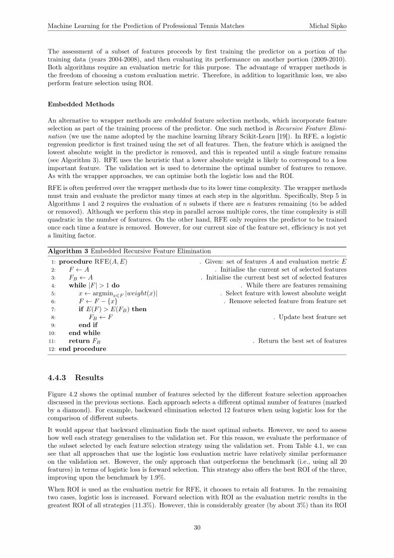
Machine Learning for the Prediction of Professional Tennis Matches Michal Sipko
The assessment of a subset of features proceeds by first training the predictor on a portion of thetraining data (years 2004-2008), and then evaluating its performance on another portion (2009-2010).Both algorithms require an evaluation metric for this purpose. The advantage of wrapper methods isthe freedom of choosing a custom evaluation metric. Therefore, in addition to logarithmic loss, we alsoperform feature selection using ROI.
Embedded Methods
An alternative to wrapper methods are embedded feature selection methods, which incorporate featureselection as part of the training process of the predictor. One such method is Recursive Feature Elimi-nation (we use the name adopted by the machine learning library Scikit-Learn [19]). In RFE, a logisticregression predictor is first trained using the set of all features. Then, the feature which is assigned thelowest absolute weight in the predictor is removed, and this is repeated until a single feature remains(see Algorithm 3). RFE uses the heuristic that a lower absolute weight is likely to correspond to a lessimportant feature. The validation set is used to determine the optimal number of features to remove.As with the wrapper approaches, we can optimise both the logistic loss and the ROI.
RFE is often preferred over the wrapper methods due to its lower time complexity. The wrapper methodsmust train and evaluate the predictor many times at each step in the algorithm. Specifically, Step 5 inAlgorithms 1 and 2 requires the evaluation of n subsets if there are n features remaining (to be addedor removed). Although we perform this step in parallel across multiple cores, the time complexity is stillquadratic in the number of features. On the other hand, RFE only requires the predictor to be trainedonce each time a feature is removed. However, for our current size of the feature set, efficiency is not yeta limiting factor.
Algorithm 3 Embedded Recursive Feature Elimination
1: procedure RFE(A,E) . Given: set of features A and evaluation metric E2: F ← A . Initialise the current set of selected features3: FB ← A . Initialise the current best set of selected features4: while |F | > 1 do . While there are features remaining5: x← argminx∈F |weight(x)| . Select feature with lowest absolute weight6: F ← F − {x} . Remove selected feature from feature set7: if E(F ) > E(FB) then8: FB ← F . Update best feature set9: end if
10: end while11: return FB . Return the best set of features12: end procedure
4.4.3 Results
Figure 4.2 shows the optimal number of features selected by the different feature selection approachesdiscussed in the previous sections. Each approach selects a different optimal number of features (markedby a diamond). For example, backward elimination selected 12 features when using logistic loss for thecomparison of different subsets.
It would appear that backward elimination finds the most optimal subsets. However, we need to assesshow well each strategy generalises to the validation set. For this reason, we evaluate the performance ofthe subset selected by each feature selection strategy using the validation set. From Table 4.1, we cansee that all approaches that use the logistic loss evaluation metric have relatively similar performanceon the validation set. However, the only approach that outperforms the benchmark (i.e., using all 20features) in terms of logistic loss is forward selection. This strategy also offers the best ROI of the three,improving upon the benchmark by 1.9%.
When ROI is used as the evaluation metric for RFE, it chooses to retain all features. In the remainingtwo cases, logistic loss is increased. Forward selection with ROI as the evaluation metric results in thegreatest ROI of all strategies (11.3%). However, this is considerably greater (by about 3%) than its ROI
30

Machine Learning for the Prediction of Professional Tennis Matches Michal Sipko
on the training set. Backward elimination using ROI, on the other hand, suffers a significant drop inperformance when evaluated on the validation set. It appears that using ROI for optimisation results inunpredictable performance on unseen data. Also, Figure 4.2b shows that different adjacent subsets (thosewith one feature added or removed) have very large differences in profit, confirming the high volatility ofROI. Logistic loss appears to be a much more stable metric. As we want to achieve the best performanceon the test set, it is imperative that the feature selection strategy we use will generalise well. For thisreason, we select forward selection with logistic loss as the optimal feature selection strategy.
Figure 4.2: Optimal feature subset sizes using different approaches
(a) Negated Logistic Loss
0 5 10 15 20
Number of features selected
−0.641
−0.640
−0.639
−0.638
−0.637
−0.636
−0.635
−0.634
−0.633
Negated
logistic
loss
Backward EliminationForward SelectionRFE
(b) Return on Investment
0 5 10 15 20
Number of features selected
0.02
0.03
0.04
0.05
0.06
0.07
0.08
0.09
0.10
ROI(using
Kelly
criterion)
Backward EliminationForward SelectionRFE
Table 4.1: Evaluation of feature selection approaches
Approach EvaluationMetric
Features Selected(in order of importance)
Performance onValidation Set
Log-loss ROI % (Kelly)
BackwardElimination log-loss
COMPLETE, WRP, W1SP, ACES,W2SP, FATIGUE, DIRECT,NA, DF, WIS, A2S, TPW
0.5764 7.1
ForwardSelection log-loss
SERVEADV, FATIGUE, DF,DIRECT, TMW, WIS, TPW,
A2S, NA, ACES, COMPLETE,WSP, W1SP
0.5743 9.7
RFE log-loss SERVEADV, TMW, DIRECT,FS, COMPLETE, W2SP, ACES
0.5765 7.0
BackwardElimination ROI COMPLETE, FS, WSP, UE,
FATIGUE, WIS, A1S0.5803 8.2
ForwardSelection ROI SERVEADV, W2SP, BP, A2S 0.5799 11.3
RFE ROI
SERVEADV, TMW, DIRECT,FS, COMPLETE, W2SP, ACES,
WRP, W1SP, UE, NA, BP,RETIRED, FATIGUE, WSP, A1S,
DF, TPW, A2S, WIS
0.5762 7.8
None All features 0.5762 7.8
31

Machine Learning for the Prediction of Professional Tennis Matches Michal Sipko
Having settled on the feature selection strategy, we now use all training and validation data (2004-2012)to generate the final feature set:
SERVEADV, DIRECT, FATIGUE, ACES, TPW, DF, BP, RETIRED, COMPLETE, NA, W1SP, A1S
The final set of features has a large overlap with the subset selected when only the training set was used.In fact, 9 of the 12 selected features were also selected previously. This suggests that the strategy willselect a relative stable subset of features as the dataset grows. We can also visualise the weights assignedto each feature by the training process. Figure 4.3 shows that SERVEADV has the greatest impact onthe outcome of the match, followed by DIRECT and ACES. As we would expect, FATIGUE, RETIRED,and DF all have negative weights. It may come as a surprise that the difference in the estimated winningon first serve percentage (W1SP) is also assigned a negative weight. However, as mentioned previously,features are not trained independently, and affect one another. Therefore, W1SP might be given anegative weight to balance out the effect of one or more of the features with positive weights.
Figure 4.3: Weights assigned to final feature set
SERVEADV
DIR
ECT
FATIG
UE
ACES
TPW DF
BP
RETIR
ED
COMPLETE
NA
W1SP
A1S
−0.2
0.0
0.2
0.4
0.6
0.8
Weigh
t
4.5 Hyperparameter Optimisation
The process of training a logistic regression predictor tunes the regression coefficients, i.e., the internalweights for each feature. However, the model also has parameters which are not optimised by the trainingprocess, termed hyperparameters. In order to achieve the best performance of the model, we optimisethese parameters using the validation set (years 2011-2012 of the dataset). To reiterate, we optimiseonly according to the performance of the least uncertain 50% of the matches in the validation set (seeSection 4.1).
4.5.1 Optimisation Approach
The most common approach to hyperparameter optimisation is grid search, a brute-force method thatexhaustively searches the entire space of different hyperparameter configurations. Most of our hyperpa-rameters are real-valued, and the tuning is fine-grained. A sufficiently fine-grained grid search would beprohibitively expensive for our purposes.
We instead proceed by a greedy heuristic search, which at any point optimises the parameter that,when altered, will cause the greatest improvement in an evaluation metric (e.g., logistic loss or ROI).We iterate until all parameters have settled in their global maxima. Since hyperparameters are notnecessarily independent, it is entirely possible that this approach will terminate in a local maximum, ormay not terminate at all. However, we found that this process worked very well for our use case.
Note that this process is intentionally not automatic, but guided by human decisions. As shown duringfeature selection, we must often trade off the optimisation of logistic loss and the optimisation of ROI.
32

Machine Learning for the Prediction of Professional Tennis Matches Michal Sipko
We expect to achieve the best results by reasoning about this trade-off for each hyperparameter andmaking a conscious decision using our knowledge of the strengths and weaknesses of each metric.
The set of features used for prediction may also be considered a model hyperparameter. Consequently,feature selection (described in the previous section) is also a part of the optimisation process. Clearly,we do not want to select features based on the performance of a very sub-optimal model. Therefore, weincorporate feature selection into the process as follows:
1. Perform an initial optimisation of hyperparameters using all features (except for RANK andPOINTS, as discussed in Section 4.4.1)
2. Run feature selection to obtain a new feature set
3. Re-optimise using the new feature set
4.5.2 Noise Removal
Our training set contains matches with varying degrees of uncertainty. Matches with very high uncer-tainty (e.g., those where the two players have very few common opponents) can be treated as noise inthe input data. By removing these matches, the predictor will be able to more accurately model the trueunderlying relationships in the dataset. We order all matches in the training set by their uncertainty,and run an optimisation to find the best percentage of higher-uncertainty matches to remove. Figure 4.4shows our results. There is a clear improvement in both ROI and logistic loss as noisy matches areremoved. We fix the hyperparameter value at 80%, the peak of the ROI. Although the logistic loss keepsimproving past 80%, there is a sharp undesirable drop in the ROI after this point.
Figure 4.4: ROI and logistic loss when removing uncertain matches
0 20 40 60 80 100
Percentage of matches removed
−0.02
0.00
0.02
0.04
0.06
0.08
0.10
0.12
ROI
−0.63
−0.62
−0.61
−0.60
−0.59
−0.58
−0.57
Negated
logistic
loss
ROI - Strategy 1ROI - Strategy 2ROI - Strategy 3Negated logistic loss
We have also considered removing training matches with noise in their output values. The bettingodds for a match could be used to identify matches that had very surprising results. We could, forexample, remove all matches for which the winner had an implied probability of winning of less than30%. However, we found that a very small number of matches were affected by such filtering, and it thushad no considerable effect on the ROI or the logistic loss.
4.5.3 Time Discount Factor
Time discounting of past matches while extracting features requires a discount factor, which is a hy-perparameter in our model. Essentially, the higher the discount factor, the lesser the effect of timediscounting. In Figure 4.5, we see that the logistic loss peaks at a discount factor of 0.8, which we selectas the optimal value. Although the ROI is maximised by using a factor of 0.9, the difference is small
33
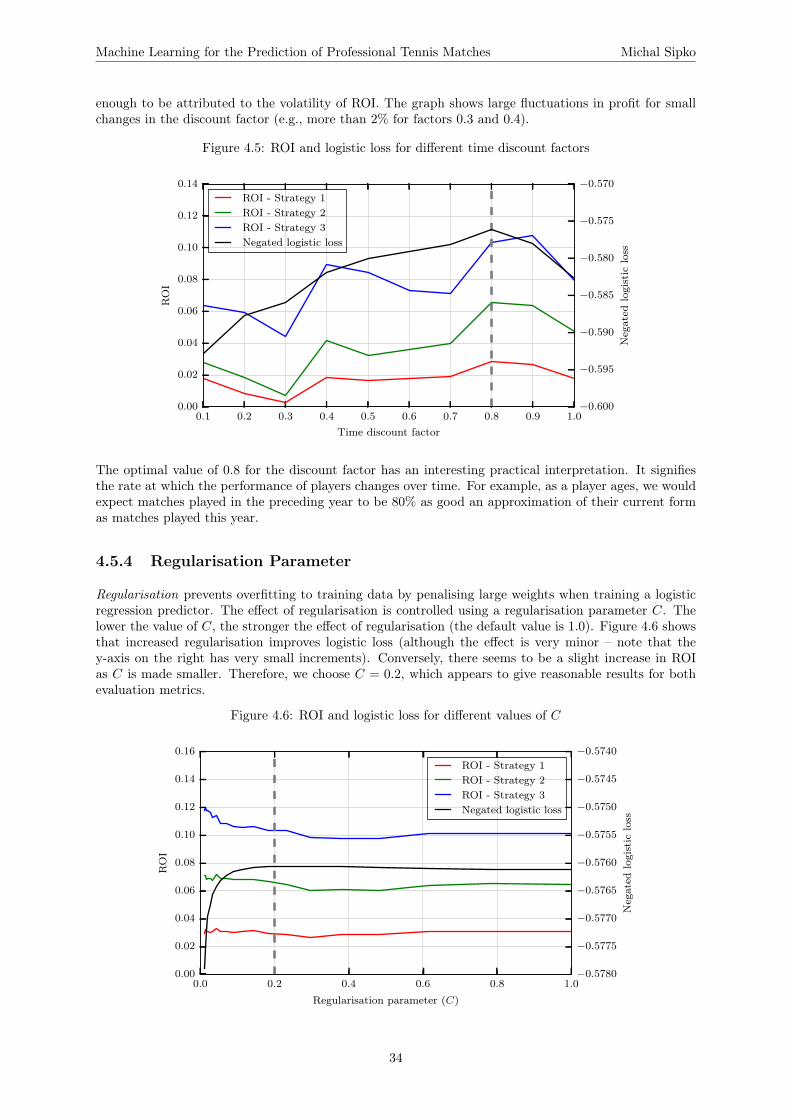
Machine Learning for the Prediction of Professional Tennis Matches Michal Sipko
enough to be attributed to the volatility of ROI. The graph shows large fluctuations in profit for smallchanges in the discount factor (e.g., more than 2% for factors 0.3 and 0.4).
Figure 4.5: ROI and logistic loss for different time discount factors
0.1 0.2 0.3 0.4 0.5 0.6 0.7 0.8 0.9 1.0
Time discount factor
0.00
0.02
0.04
0.06
0.08
0.10
0.12
0.14
ROI
−0.600
−0.595
−0.590
−0.585
−0.580
−0.575
−0.570
Negated
logistic
loss
ROI - Strategy 1ROI - Strategy 2ROI - Strategy 3Negated logistic loss
The optimal value of 0.8 for the discount factor has an interesting practical interpretation. It signifiesthe rate at which the performance of players changes over time. For example, as a player ages, we wouldexpect matches played in the preceding year to be 80% as good an approximation of their current formas matches played this year.
4.5.4 Regularisation Parameter
Regularisation prevents overfitting to training data by penalising large weights when training a logisticregression predictor. The effect of regularisation is controlled using a regularisation parameter C. Thelower the value of C, the stronger the effect of regularisation (the default value is 1.0). Figure 4.6 showsthat increased regularisation improves logistic loss (although the effect is very minor – note that they-axis on the right has very small increments). Conversely, there seems to be a slight increase in ROIas C is made smaller. Therefore, we choose C = 0.2, which appears to give reasonable results for bothevaluation metrics.
Figure 4.6: ROI and logistic loss for different values of C
0.0 0.2 0.4 0.6 0.8 1.0
Regularisation parameter (C)
0.00
0.02
0.04
0.06
0.08
0.10
0.12
0.14
0.16
ROI
−0.5780
−0.5775
−0.5770
−0.5765
−0.5760
−0.5755
−0.5750
−0.5745
−0.5740
Negated
logistic
loss
ROI - Strategy 1ROI - Strategy 2ROI - Strategy 3Negated logistic loss
34

Chapter 5
Higher Order Models
5.1 Bias and Variance
Errors in the predictions of tennis match outcomes can be classified into two categories: those due tobias and those due to variance. Bias results from erroneous assumptions of the model, i.e., its inabilityto accurately capture the relationships in the data (under-fitting). For example, we may be missingsome important match features, and for this reason our predictions may be systematically wrong. Onthe other had, variance is the sensitivity of the model to small variations in the dataset. A model withhigh variance does not generalise well to unseen data (overfitting). There is always a trade-off betweenbias and variance. A more complex model can more accurately capture relationships in the data, but itwill not generalise as well.
Model variance can typically be reduced by using a larger dataset, since the model will then be lesslikely to overfit to noise in the data. Figure 5.1 shows that the predictive power of our logistic regressionmodel is relatively constant when we vary the size of the training dataset. The best return on investmentoscillates between 8% and 10% and the error, as measured by logistic loss, actually grows (althoughvery slightly) with more training data. These results suggest that our model has low variance, andto improve its performance, we could attempt to reduce the bias. The following sections present twodifferent approaches to increasing the expressiveness of the model.
Figure 5.1: ROI and logistic loss on validation set for different training set sizes
1 2 3 4 5 6 7
Years of data used for training
0.00
0.02
0.04
0.06
0.08
0.10
0.12
0.14
ROI
−0.580
−0.578
−0.576
−0.574
−0.572
−0.570
Negated
logistic
loss
ROI - Strategy 1ROI - Strategy 2ROI - Strategy 3Negated logistic loss
35

Machine Learning for the Prediction of Professional Tennis Matches Michal Sipko
5.2 Logistic Regression with Interaction Features
5.2.1 Constuction of Interaction Features
Logistic regression is a generalised linear model. As described in Section 2.5.2, it computes the probabilityof a match outcome using the weighted sum of the values of the match features:
P (Player 1 wins) = σ(z) =1
1 + e−z
Wherez = β1x1 + β2x2 + · · ·+ βnxn, βi is the weight for feature xi
For this reason, the model can only fit a linear decision boundary to the feature space and higher-orderrelationships between the features cannot be represented. A common approach to allowing a non-lineardecision boundary is the introduction of interaction terms, the weighted products of features. Afteradding interaction terms, z becomes:
z =
original terms︷ ︸︸ ︷β1x1 + β2x2 + · · ·+ βnxn +
interaction terms︷ ︸︸ ︷β12x1x2 + β13x1x3 + · · ·+ β(n−1)nxn−1xn
In total, there are(n2
)additional features, one for each unique product of two of the original features. This
model can now identify higher-order relationships in the data, resulting in lower model bias. However,increasing the complexity of the model will increase its variance, making it more prone to overfitting.Also, both the training and optimisation of the model will be more computationally expensive.
We have already extracted one interaction feature: COMPLETE. Completeness for player i was definedas the product of their serve and return strengths (WSPi ·WRPi). Notice that we compute the productbefore taking the difference in the values of the two players. This is a distinction between our approachand the standard application of interaction features. In general, the interaction feature A_B, based onfeatures A and B, is computed as follows:
A_Bi = Ai · Bi
A_B = A_B1 − A_B2
We have decided to exclude any interaction features formed using the RETIRED value for a player, dueto its binary nature (it would either invert the sign of the other multiplicand or have no effect). Thisgives us with a total of
(192
)+ 20 = 173 features.
5.2.2 Model Optimisation
A larger feature set increases the likelihood of our model overfitting to noise in the training data. Asbefore, we can run a feature selection algorithm to select a subset of features with the best performance. Itis essential that the chosen algorithm generalises well, so we re-evaluate all three approaches (backwardelimination, forward selection, and RFE) using the new, higher-order model. As evaluating subsetsusing ROI previously failed to generalise well, we only use logistic loss to compare different subsets.Figure 5.2 shows the results of running the three feature selection strategies on the training set. Backwardelimination selects a far greater number of features than the other approaches (57), but this subset hasthe best performance on the training set. Note that during feature selection, the model hyperparametersare set to the most optimal values derived for the basic logistic regression model in Section 4.5.
Table 5.1 shows that the feature subsets selected by the three approaches result in similar logistic losswhen evaluated on the validation set. The only approach that improves upon the benchmark (i.e., usingall features) in terms of logistic loss is backward elimination. Although the best ROI is achieved by thebenchmark, the difference is very minor in comparison to backward elimination. Therefore, we selectbackward elimination as the feature selection strategy.
The final feature set for use by the model is selected by running backward elimination on all trainingand validation data. This time, only 19 features are selected. Furthermore, as shown in Figure 5.3, all
36

Machine Learning for the Prediction of Professional Tennis Matches Michal Sipko
Figure 5.2: Feature selection with polynomial features
0 20 40 60 80 100 120 140 160 180
Number of features selected
−0.67
−0.66
−0.65
−0.64
−0.63
−0.62
Negated
logistic
loss
Backward EliminationForward SelectionRFE
Table 5.1: Evaluation of feature selection approaches
Approach Number of featuresselected
Performance onValidation Set
Log-loss ROI % (Kelly)
BackwardElimination 57 0.5737 8.2
ForwardSelection 23 0.5753 7.8
RFE 6 0.5775 6.3
None All features (173) 0.5745 8.4
but two of the selected features are interaction features (ACES and RETIRED are the only two “original”features in the selected subset). Interestingly, ACES has replaced SERVEADV as the feature with thegreatest weight. The meaning of many selected interaction features is difficult to grasp, and some seemcompletely non-sensical. For example, the large negative weight assigned to ACES_W2SP suggests thata player that hits many aces and has strong performance on their second serve is less likely to win.However, the weights of different features should not be considered independently, as they affect oneanother. For example, it is entire possible that ACES_W2SP would be assigned a positive weight ifsome additional features were removed. With the addition of interaction features, the model has becometoo complex to allow for an interpretation of the assigned weights.
A different feature set may require the re-optimisation of the model hyperparameters. However, theoptimal value of only a single hyperparameter affected by the introduction of interaction features: theregularisation parameter C. We decided to decrease the value of C from 0.2 to 0.1, implying that thehigher-order model performs slightly better with stronger regularisation. This is consistent with ourexpectations. Regularisation reduces the variance of a model, so a more variable model, as obtained bythe introduction of interaction features, will benefit from stronger regularisation.
5.3 Artificial Neural Network
In the previous section, we have attempted to decrease the model bias by introducing additional featuresin a logistic regression predictor. These features allow the representation of more complex relationshipsin the data. However, the approach is clearly not scalable. Modelling interactions between triples offeatures would necessitate
(193
)= 969 additional features. Such a model would be highly susceptible to
overfitting, and our feature selection approaches would no longer be feasible.
37

Machine Learning for the Prediction of Professional Tennis Matches Michal Sipko
Figure 5.3: Weights assigned to final feature set (logistic regression with interaction features)
TPW
_W
SP
TMW
_A2S
W2SP_DIR
ECT
TPW
_A2S
WRP_BP
DF_W
SP
DF_BP
NA_DIR
ECT
TPW
_UE
BP_UE
BP_A2S
ACES
NA_SERVEADV
ACES_W
2SP
RETIR
ED
TPW
_FATIG
UE
WRP_NA
ACES_UE
−0.6
−0.4
−0.2
0.0
0.2
0.4
0.6
0.8Weigh
t
An alternative approach involves the use of an artificial neural network (described in Section 2.5.3).ANNs can model highly complex functions of the input features. The output values of neurons in thehidden layer may be influenced by many (or all) of the features. Such a representation may uncoversignificant relationships between the features, which would be ignored in a lower-dimensional model.However, the use of ANNs brings new challenges. Firstly, ANNs take significantly longer to train thanlogistic regression models. On our dataset, a logistic regression model took at most several seconds totrain, while a neural network takes 10 minutes or more, depending on the hyperparameters. The modelconfiguration is also more difficult, and forms an active research area. There are many hyperparametersto optimise (structure of the network, learning rate, momentum, etc.), and many parameters have strongdependencies on the values of other parameters.
The task of training a neural network for tennis match prediction has been attempted by Somboon-phokkaphan et al. [22]. There are some essential differences in comparison to our model. Firstly, theauthors used a simple averaging approach to feature extraction, without surface weighting or time dis-counting. Instead, the surface was fed as an additional input feature to the network (i.e., a binary inputnode for each possible surface). More importantly, separate input features were used for the averagestatistics of the two players, in contrast to our features of differences (Section 3.1.2), introducing asym-metry into the model. In addition, there is no mention of feature standardisation and mean-centering(which would be beneficial in this case). Although the authors claim an average accuracy of about 75%in predicting the matches in the Grand Slam tournaments in 2007 and 2008, there is no assessment of theactual probabilities predicted (using ROI or a scoring rule such as logarithmic loss). We have attemptedto replicate the experiment as described in the paper, but we were unable to reproduce the results.
5.3.1 Network structure
To reduce the size of the hyperparameter space, we fix some aspects of the structure of the networkheuristically. The overall architecture of the network is that of a multilayer perceptron (MLP), a feed-forward network trained by backpropagation. We use all features (except for rank-related information)as inputs. The filtering of training data based on uncertainty and the time discount factor are set totheir optimal values for logistic regression (80% and 0.8, respectively).
We use a single hidden layer. Hornik [10] showed that a single hidden layer with a finite number of neuronscan approximate any continuous function, provided that a sufficient number of hidden neurons is used. Itis generally accepted that a single layer is sufficient for most networks. However, as shown in Figure 5.4,the number of neurons in the hidden layer remains a hyperparameter that we must optimise.
The most common activation functions are sigmoid “squashing” functions. One such function is thelogistic function, which has a range of [0, 1], and is also used in logistic regression. An alternative is the
38

Machine Learning for the Prediction of Professional Tennis Matches Michal Sipko
hyperbolic tangent (tanh) function, with a range of [−1, 1]. LeCun [14] argues that symmetric sigmoidssuch as the tanh function result in lower training times, so we use the tanh activation function in ourhidden neurons. However, the final value returned by an activation of the network (i.e., the output ofthe single neuron in the output layer) must be interpretable as a valid probability. For this reason, weuse the logistic function for activation in the output neuron (an alternative approach would be to usetanh in the output neuron, and then remap the outputs to valid probabilities).
Conventionally, a network contains a bias neuron, which is connected to every non-input node in thenetwork. The bias neuron always emits a constant value (e.g., 1), and allows a horizontal shift in theactivation functions of individual neurons. However, as explained in Section 3.1.2, we strive to obtaina symmetric model, i.e., one that would give the same prediction if the players were labelled in reverse.By excluding the bias neuron, we are ensuring that the network is unable to give an unfair advantageto either player. In other words, if all input features are zero (the players are expected to have identicalperformance), the network output (the probability of Player 1 winning) is guaranteed to be exactly 0.5,regardless of the weights assigned by backpropagation. Furthermore, the exclusion of bias reduces thecomplexity of the network and thus helps prevent overfitting.
Figure 5.4: ANN architecture
...
...
ACES
DF
WSP
FATIGUE
H1
Hn
P (Player 1 win)
Input layer(20 nodes)
Hidden layer(tanh activation)
Output layer(logistic activation)
5.3.2 Model optimisation
We adopt the same approach to hyperparameter optimisation as for logistic regression: at each step,we optimise a single parameter (based on its performance on the validation set) and then re-run theanalysis for the remaining parameters. This iterative process is more difficult this time, since the hyper-parameters have stronger dependencies. For example, changing the learning rate requires re-calibratingregularisation, momentum, etc.
Number of hidden nodes
The number of hidden nodes affects the generalisation ability of a network. A network with a high numberof hidden nodes has higher variance, and is therefore more likely to overfit to the training data. Too fewhidden nodes, on the other hand, can result in high bias. There are various heuristics for selecting thenumber of hidden nodes, based on the number of training examples and the number of input / outputnodes. Different sources advocate different “rules of thumb”, and there seems to be little consensus inthe matter. Sarle [21] claims that these rules are “non-sense”, since they ignore the amount of noise inthe data and the complexity of the function being trained. They also do not take into consideration the
39

Machine Learning for the Prediction of Professional Tennis Matches Michal Sipko
amount of regularisation and whether early stopping is used. Sarle suggests that in most situations, theonly way determine the optimal number of hidden units is by training several networks and comparingtheir generalisation errors.
Figure 5.5: ROI and logistic loss for different numbers of nodes in hidden layer
0 50 100 150 200
Number of nodes in hidden layer
0.00
0.02
0.04
0.06
0.08
0.10
0.12
0.14
0.16
0.18
ROI
−0.62
−0.61
−0.60
−0.59
−0.58
−0.57
−0.56
Negated
logistic
loss
ROI - Strategy 1ROI - Strategy 2ROI - Strategy 3Negated logistic loss
As shown in Figure 5.5, the profit is highly variable for networks of different sizes, oscillating between8% and 10% when betting with Strategy 3. However, the logistic loss seems to improve with the numberof nodes, especially when the number of nodes is less than 50. There does not seem to any significantbenefit of having more than 100 nodes, and since it is in our interest to keep the network as small aspossible (to reduce variance and training time), we fix the value of this parameter at 100.
Learning rate
The learning rate parameter determines the extent to which the current training set error affects theweights in the network at each training epoch. A higher learning rate results in faster convergence,but due to the coarser granularity of the weight updates, it may prevent the learning algorithm fromconverging to the optimal value. We can illustrate this by plotting learning curves for different learningrates, which show the evolution of the training and validation set errors during the training process(Figure 5.6). A learning rate of 0.0001 takes more than three times as long to converge as a learning rateof 0.0004. Also, the error on the validation set, as measured by logistic loss, actually slightly decreasesfrom 0.5798 from 0.5795 when 0.0004 is used. A further increase in the learning rate (to 0.0008) resultsin a less significant improvement in training time and an increase in logistic loss. Therefore, we select0.0004 as the learning rate.
Figure 5.6: Learning curves for different learning rates
0 200 400 600 800 1000
Epochs
0.10
0.12
0.14
0.16
0.18
0.20
R2
log-loss: 0.5798
0.0001
0 200 400 600 800 1000
Epochs
log-loss: 0.5796
0.0002
0 200 400 600 800 1000
Epochs
log-loss: 0.5795
0.0004
0 200 400 600 800 1000
Epochs
log-loss: 0.5800
0.0008
TrainValidation
40

Machine Learning for the Prediction of Professional Tennis Matches Michal Sipko
The learning rate does not need to remain constant during training. An adaptive learning rate canchange during training so as to take smaller steps when converging to a value. One such approach islearning rate decay, which exponentially shrinks the learning rate during training. Although we havenot attempted to incorporate adaptive learning rates into the model (to minimise the hyperparametersearch space), this is a possible future improvement of the model.
Regularisation
Regularisation in neural networks can be achieved through weight decay, the exponential shrinkage ofweights during training. For example, a weight decay parameter of 0.01 means that that the updatedweights are shrunk by one percent during each training epoch. This prevents weights from becomingvery large, which helps avoid overfitting. The approach is analogous to the C parameter in logisticregression.
Figure 5.7: ROI and logistic loss for varying weight decay
0.002 0.004 0.006 0.008 0.010 0.012 0.014 0.016 0.018 0.020
Weight decay
0.00
0.02
0.04
0.06
0.08
0.10
0.12
ROI
−0.590
−0.588
−0.586
−0.584
−0.582
−0.580
−0.578
−0.576
Negated
logistic
loss
ROI - Strategy 1ROI - Strategy 2ROI - Strategy 3Negated logistic loss
In Figure 5.7, we can see that the error on the validation set grows with increased regularisation. Thismeans that the decay of weights prevents the predictor for modelling relationships in the dataset asaccurately. However, we can also see a clear upward trend in the return on investment. As we increasethe weight decay from 0.002 to 0.02, the ROI grows by over 3%. Further analysis shows that thetrend continues even for unreasonably large values of weight decay: stronger regularisation results inhigher profits, despite greater logistic loss. This counter-intuitive phenomenon can be explained asfollows: strong regularisation forces the weights in the network to be smaller and therefore the predictedprobabilities are more moderate (i.e., closer to 0.5). As a result, bets are only placed on matches witha greater mis-pricing of the odds, resulting in greater profits. Notice that Strategy 1 (betting on thepredicted winner) is unaffected by the magnitude of the probability values and thus remains constant withstronger regularisation. This graph would suggest maximising regularisation to achieve the maximumreturns. However, stronger regularisation also reduces the number of bets placed by Strategies 2 and 3,and the amount wagered by Strategy 3. If an investor re-invests their profits into subsequent matches,a higher frequency of bets results in exponentially higher returns. This notion of compounding is notmeasurable by ROI, which assumes a fixed bet size, regardless of change in the investor’s bankroll.
Our goal is to predict the most accurate probabilities for the outcomes of matches. In this situation,optimising for the greatest ROI degrades the quality of the predictions. We aim to obtain a distributionof predicted probabilites that is similar to the distribution of true probabilities. Figure 5.8 shows thatincreasing the regularisation makes the distribution of predicted probabilities narrower. If we approxi-mate the true probability distribution by the distribution of probabilities implied by betting odds, wesee that it has a larger standard deviation than any of our predicted probability distributions. To obtainthe most realistic probability estimates, we should therefore minimise the weight decay. We find that a
41

Machine Learning for the Prediction of Professional Tennis Matches Michal Sipko
weight decay of less than 0.002 results in very inconsistent behaviour. Therefore, we choose 0.002 as thevalue for the weight decay parameter.
Figure 5.8: Distributions of predicted probabilities for varying weight decay
0.0 0.2 0.4 0.6 0.8 1.0
P (Player 1 win)
0
100
200
300
400
500
600
700
Num
berof
matches
σ = 0.1999
Decay: 0.002
0.0 0.2 0.4 0.6 0.8 1.0
P (Player 1 win)
σ = 0.1633
Decay: 0.02
0.0 0.2 0.4 0.6 0.8 1.0
P (Player 1 win)
σ = 0.1054
Decay: 0.05
0.0 0.2 0.4 0.6 0.8 1.0
P (Player 1 win)
σ = 0.2354
Implied probabilities
Bagging
The training process of a neural network begins with randomly initialised weights. Therefore, the sametraining dataset can produce networks with very different weights and thus different levels of performance.We wish to reduce this variability to ensure that the model performs well on the test set. Bootstrapaggregating (also known as bagging) is an approach for stabilising the performance of machine learningmodels by combining multiple versions of a predictor into a single aggregate predictor. First, we generaten bootstrap datasets from the original training dataset by sampling from the dataset uniformly and withreplacement. Each bootstrap dataset has the same number of examples as the original, but only about1− 1
e of the examples are expected to be unique, with the rest being duplicates. We then train a differentneural network using each bootstrap dataset. To predict the outcome of a match, we take the mean ofthe predictions of the n neural networks. Breiman [4] showed that bagging can provide significant gainsin accuracy, especially when the underlying predictor is unstable.
Figure 5.9: ROI and logistic loss for different numbers of bootstrap datasets
0 5 10 15 20
Number of bootstrap datasets
0.00
0.02
0.04
0.06
0.08
0.10
0.12
ROI
−0.586
−0.584
−0.582
−0.580
−0.578
−0.576
−0.574
−0.572
Negated
logistic
loss
ROI - Strategy 1ROI - Strategy 2ROI - Strategy 3Negated logistic loss
42

Machine Learning for the Prediction of Professional Tennis Matches Michal Sipko
It remains to decide the number of bootstrap datasets (n). Breiman used 25 datasets in his experiments,and most of the improvement in prediction accuracy was gained from only 10 datasets. By evaluatingthe performance of models with different numbers of bootrap datasets (Figure 5.9), we find that there isa significant improvement in performance when the number of bags is increased from 1 to 8. However,adding more than 10 bootstrap datasets appears to make little difference. Nevertheless, we expect thepredictions to be more stable with a larger number of predictors, so we can train as many as possible,considering a reasonable amount of compute resources is used. In the evaluation, we train 20 individualpredictors.
Other Parameters
We use the online learning variation of backpropagation, which updates weights immediately after beingpresented each training example. The alternative is batch learning, which only updates weights at the endof each epoch, having seen all training examples. In theory, batch learning should result in more accurateadjustments to weight, at the expense of longer training times. However, Wilson and Martinez [23] arguethat this is a “widely held myth” in the neural network community, and that convergence can be reachedsignificantly faster with online learning, with no apparent difference in accuracy. An investigation intobatch learning could be conducted in the future.
Momentum can be added to the learning process to avoid local minima and, according to LeCun [14],speed up convergence. When momentum is used, a fraction of the previous weight update is incorporatedin the current update during training. In this way, we avoid large fluctuations in the directions ofweight updates. Although momentum did not have a significant impact on the prediction accuracy, weempirically found that a momentum coefficient of 0.55 resulted in much faster convergence.
It is necessary to define the stopping criteria for training. We use a common technique called earlystopping [20], which uses a validation set to detect when overfitting begins to occur. Note that we donot use our validation set (years 2010-2011) for this purpose, but instead split the training set into twoportions, one for training and one for early stopping. We conclude the training process when the erroron the validation set does not achieve a new minimum for 10 consecutive epochs.
43

Chapter 6
Implementation Overview
6.1 Data Flow
The first step in the implementation of a machine learning predictor for tennis match outcomes is thegeneration of the dataset. As discussed in Section 2.2, we obtain raw historical tennis data from theOnCourt system. SQL queries are run against the OnCourt MySQL database to retrieve all informationnecessary for feature extraction. Next, we process the data to generate the dataset, as described inChapter 3. The generated dataset is persisted as a CSV (comma-separated values) file.
Each machine learning algorithm reads the dataset file prior to training. The dataset is divided asdescribed in Section 4.1, and the model is first trained and then tested on separate parts of the dataset.Finally, the results of the evaluation are also saved in a file.
Figure 6.1: Data flow diagram
6.2 Technologies
All data processing components of the system were implemented in the Python1 programming language.Python has several packages for scientific computing which have made the implementation succinct andefficient, in particularNumPy2 andPandas3. These two libraries provide a clean interface to in-memorymanipulation of large datasets.
For logistic regression, we use the machine learning library scikit-learn4. This library also providesuseful utility functions for machine learning, such as grid search. However, it does not have an imple-mentation for artificial neural networks. For this purpose, we utilise PyBrain5, the library recommendedby scikit-learn. Both machine learning libraries are Python-based.
1http://www.python.org/2http://www.numpy.org/3http://pandas.pydata.org/4http://scikit-learn.org/5http://pybrain.org/
44

Machine Learning for the Prediction of Professional Tennis Matches Michal Sipko
The data processing is done in an Ubuntu virtual machine hosted on the private cloud6 of the Departmentof Computing at Imperial College. The VM has 8×3 GHz processors and 16 GB RAM. The entire systemruns inside a Docker7 container, for portability between VMs. Git8 is used for version control.
6.3 Efficiency
We have no requirements for the efficiency of the system, provided that a prediction can be generated intime for an upcoming match with a reasonable amount of resources (compute power / memory).
The most demanding part of the data flow (by a large margin) is the generation of the dataset, whichtakes over 10 hours. The long processing time can be attributed to the common opponent featureextraction approach, which requires assessing the performance of both players in every match relative toall their common opponents. However, once generated, adding additional data points (i.e., new completedmatches) is a matter of minutes, as is the training of a predictor. Therefore, the current architecture ofthe system is efficient enough to allow for betting on upcoming matches.
6http://www.doc.ic.ac.uk/csg/services/cloud7http://www.docker.com/8http://git-scm.com/
45

Chapter 7
Evaluation
7.1 Evaluation Method
Having trained different machine learning based models for the prediction of tennis matches, we nowcompare how they perform on unseen data. As described in Section 4.1, we have split our dataset intothree divisions: training, validation, and test. We draw attention to the fact that the test data has notbeen used for any purpose before this point, and is therefore a valid approximation for new, upcomingmatches.
Throughout the evaluation, as during the optimisation of the models, we only consider the models’performance on the least uncertain 50% of the matches. This gives us a more representative quantificationof a model’s performance, since the result is less affected by poor predictions caused by a lack of data.In reality, we would only bet on the matches whose features are based on a sufficient amount of data, soit makes sense to evaluate the performance of the models with respect to these matches.
We use odds from the bookmaker Pinnacle1 for all ROI calculations. According to comparisons ofdifferent bookmakers2, Pinnacle offers the best payout on almost all events, so the odds will give us arealistic ROI estimate. After removing 50% of the matches based on uncertainty, our test set contains6315 ATP matches with Pinnacle odds, played during the years 2013-2014.
We use Knottenbelt’s Common-Opponent model [13] as the benchmark for comparison (see Section 2.4.4).The stochastic model represents the current state-of-the-art in tennis modelling, and it is our ambitionto improve upon its performance.
7.2 Results
7.2.1 ROI and Logistic Loss
Figure 7.1 shows the return on investment when betting on the matches in the test set using differentbetting strategies (the three strategies are detailed in Section 2.3.2). All strategies are profitable for allmodels. Strategy 3, which bets on the predicted winner according to the Kelly criterion, has the bestperformance. Furthermore, all three machine learning models are considerably more profitable thanthe benchmark when this strategy is used, improving the ROI by about 75%. Interestingly, althoughtheir performance is very similar when using Strategy 3, the basic logistic regression model performsmuch better than the other ML models for the remaining strategies. This could be due to the subset ofselected features used in this model, which differs from the others.
During hyperparameter optimisation, we noticed that the ROI was a very unstable evaluation metric(small changes in parameter configurations would result in large changes in ROI). For this reason, we alsocompare the prediction error of the different models (measured by logistic loss), which is less volatile.
1http://www.pinnaclesports.com/2http://www.oddsportal.com/odds-quality/
46

Machine Learning for the Prediction of Professional Tennis Matches Michal Sipko
Figure 7.1: Percentage return on investment on test set for different betting strategies
Logistic Regression Log. Reg. (Interaction) ANN Common-Opponent0
1
2
3
4
5ROI(%
)
1.46
0.73 0.70
0.20
3.62
1.692.07 1.89
4.17 4.084.35
2.40
Strategy 1Strategy 2Strategy 3
Figure 7.2 shows the error on both the validation and test sets for all models. As expected, the erroris greater on the test set than on the validation set for the ML models, since their hyperparameterswere optimised to achieve the best performance on the validation set, resulting in some overfitting. Themodel most prone to overfitting appears to be the logistic regression model with interaction features.The model had a much lower error on the validation set than the other models, but its performance onthe test set is very similar to that of the basic logistic regression model. This overfitting is most likelya result of the feature selection process. Only 18 of 173 features were selected, based on the validationset. With the high dimensionality of the feature space, it is possible that some of these features have notrue correspondence with match outcomes.
It is interesting to note that the error also increases for the Common-Opponent model. Since no op-timisation was conducted for the Common-Opponent model using the validation set, we would expectit to perform just as well on both sets of data. The increased error of this model for matches playedin the years 2013-2014 suggests that these matches might have simply been more difficult to predict(based on historical statistics) than those in the years 2011-2012. Perhaps players are becoming evermore inconsistent.
Figure 7.2: Logistic loss on the validation and test sets
Logistic Regression Log. Reg. (Interaction) ANN Common-Opponent0.56
0.58
0.60
0.62
0.64
0.66
Log
isticloss
0.5761 0.57270.5766
0.5895
0.6129 0.6122 0.6111
0.6228
ValidationTest
If we consider the test set error in Figure 7.2, we see that for the ML models, the error slightly decreaseswith increased complexity. In other words, the ANN-based model, which can express the most complexrelationships between the input features, also has the lowest test error (and the highest ROI). Dueto the immense number of training examples, we can decrease the bias of a machine learning tennispredictor without a significant increase in variance. This suggests that further improvement could beachieved by an even greater increase in the model’s complexity (e.g., by constructing additional relevantfeatures).
47

Machine Learning for the Prediction of Professional Tennis Matches Michal Sipko
7.2.2 Betting Volume
A limitation of ROI as an evaluation metric is its ignorance of the betting volume for different models. Amodel that bets only on 10 matches in the test set and has an ROI of 10% is clearly inferior to a modelthat bets on 20% of the matches and offers the same ROI. All three betting strategies use a fixed-sizemaximum bet. However, in practice, this bet limit can be adjusted according to the current size of abettor’s bankroll. In this way, the returns from previous matches can be re-invested into (larger) betson future matches. A model which generates predictions that result in larger or more frequent betswill provide exponentially higher returns. It is therefore important to also compare this aspect of themodels.
Table 7.1: Betting volume (based on Strategy 3)
Model Bets placed Investment Return Net profit
Logistic regression 3181 709.53 739.12 29.59Logistic reg. (interaction features) 3140 670.69 698.08 27.39Artificial neural network 3183 695.60 725.85 30.26Common-opponent 2515 489.10 500.84 11.75
Table 7.1 shows that the models based on machine learning place a significantly larger number of betswhen betting with Strategy 3 (the most profitable strategy for all four models). For example, the ANNbets on over 50% of the 6315 matches we are considering, while the benchmark bets on less than 40%.Furthermore, the amount invested is increased by about 43% when the ANN model is used. The MLmodels are considerably more effective at finding opportunities for placing bets, despite using the samebetting strategy as the Common-Opponent model.
Why does the Common-Opponent model place fewer bets? Figure 7.3 reveals that the distribution ofpredicted probabilities for the Common-Opponent model has a much smaller standard deviation thanthe distributions of the other models (0.16% versus 0.20%, respectively). In other words, the stochasticmodel tends to assign less extreme probabilities to match outcomes. The betting strategy only placesa bet if the predicted probability of a player winning a match is greater than the implied probability.Clearly, with lower probabilities, there will be fewer such cases. It may be possible to correct thissystematic error in the Common-Opponent model (we have set all parameter values to those given in thepublication). However, even if the Common-Opponent model had a wider distribution, we would stillexpect better performance from the ML models. All three ML models offer significantly higher returnseven when Strategy 1 is used for betting (see Figure 7.1), and this strategy is unaffected by the standarddeviation of the probability distribution.
Figure 7.3: Predicted probability distributions for different models
0 5 10 15 20
P (Player 1 win)
0
200
400
600
800
1000
Num
berof
matches
σ = 0.2005
Logistic Regression
0 5 10 15 20
P (Player 1 win)
σ = 0.2002
Log. Reg. (Interaction)
0 5 10 15 20
P (Player 1 win)
σ = 0.2029
ANN
0 5 10 15 20
P (Player 1 win)
σ = 0.1573
Common-Opponent
48
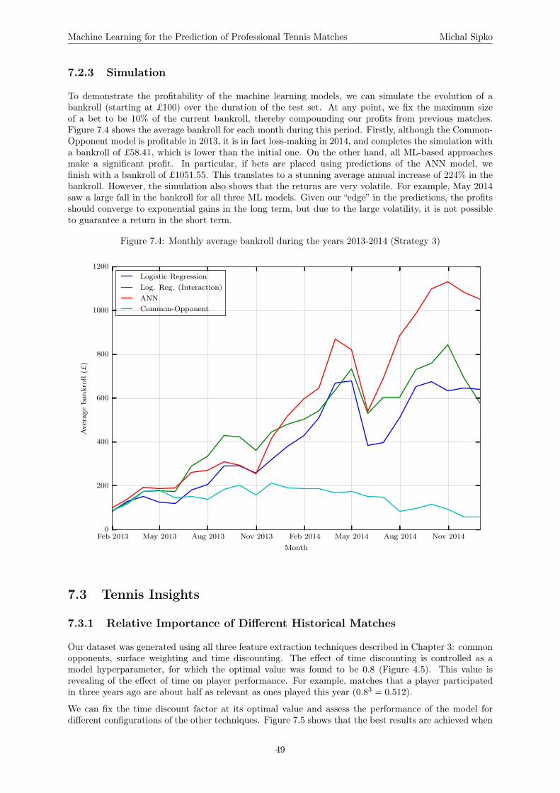
Machine Learning for the Prediction of Professional Tennis Matches Michal Sipko
7.2.3 Simulation
To demonstrate the profitability of the machine learning models, we can simulate the evolution of abankroll (starting at £100) over the duration of the test set. At any point, we fix the maximum sizeof a bet to be 10% of the current bankroll, thereby compounding our profits from previous matches.Figure 7.4 shows the average bankroll for each month during this period. Firstly, although the Common-Opponent model is profitable in 2013, it is in fact loss-making in 2014, and completes the simulation witha bankroll of £58.41, which is lower than the initial one. On the other hand, all ML-based approachesmake a significant profit. In particular, if bets are placed using predictions of the ANN model, wefinish with a bankroll of £1051.55. This translates to a stunning average annual increase of 224% in thebankroll. However, the simulation also shows that the returns are very volatile. For example, May 2014saw a large fall in the bankroll for all three ML models. Given our “edge” in the predictions, the profitsshould converge to exponential gains in the long term, but due to the large volatility, it is not possibleto guarantee a return in the short term.
Figure 7.4: Monthly average bankroll during the years 2013-2014 (Strategy 3)
Feb 2013 May 2013 Aug 2013 Nov 2013 Feb 2014 May 2014 Aug 2014 Nov 2014Month
0
200
400
600
800
1000
1200
Average
bank
roll(£
)
Logistic RegressionLog. Reg. (Interaction)ANNCommon-Opponent
7.3 Tennis Insights
7.3.1 Relative Importance of Different Historical Matches
Our dataset was generated using all three feature extraction techniques described in Chapter 3: commonopponents, surface weighting and time discounting. The effect of time discounting is controlled as amodel hyperparameter, for which the optimal value was found to be 0.8 (Figure 4.5). This value isrevealing of the effect of time on player performance. For example, matches that a player participatedin three years ago are about half as relevant as ones played this year (0.83 = 0.512).
We can fix the time discount factor at its optimal value and assess the performance of the model fordifferent configurations of the other techniques. Figure 7.5 shows that the best results are achieved when
49

Machine Learning for the Prediction of Professional Tennis Matches Michal Sipko
both common opponents and surface weighting by correlation are used together, as we have done. Whenno distinction is made between surfaces and averages are computed across all past matches, the logisticregression predictor has very poor performance, making a loss of over 6%. Interestingly, without commonopponents, splitting by surface is more profitable than weighting by surface correlation. However, whencombined with common opponents, splitting by surface performs worse. This is most likely because itresults in very few matches being available for computing averages. For example, if a match is playedon grass, it is entirely possible that the players have no (reasonably recent) common opponents on thissurface. From these results, we can claim that a player’s performance is heavily dependent on the surface,and a model is likely to have significantly better accuracy when the surface is taken into account.
Figure 7.5: Evaluation of feature extraction techniques (logistic regression)
C, S C, W C S W NoneFeature extraction technique
−8
−6
−4
−2
0
2
4
6
ROI(%
)
ROI - Strategy 1ROI - Strategy 2ROI - Strategy 3
C− Common opponentsS− Split by surface
W − Weight by surface correlations
7.3.2 Relative Importance of Different Features
As part of our investigation into tennis prediction with machine learning, we hoped to get an insight intothe relevance of different features. By inspecting the weights assigned by logistic regression (Figure 4.3),we see that the single most important feature is SERVEADV, the difference in the players’ advantageon serve. In fact, this is also the first feature to be chosen during feature selection using the forwardselection algorithm. The importance of this feature is unsurprising, since it considers the most importantqualities of the two players: their serve and return strengths. The weights in the logistic regression modelalso show that many of the features we constructed – DIRECT, FATIGUE, RETIRED and COMPLETE– affect the outcome of the match. The head-to-head balance of the players, modelled by the DIRECTfeature, seems particularly important, and is not considered by the stochastic Common-Opponent model.For the author, it comes as a surprise that the ACES feature has a very high weight in both logisticregression models. This shows that powerful serves are essential to winning matches.
Unfortunately, the higher-order models give us little insight into the relative importance of differentfeatures. The limitations of such “black boxes” are discussed in the next section.
50

Machine Learning for the Prediction of Professional Tennis Matches Michal Sipko
7.4 Limitations
7.4.1 Black Box Models
The stochastic tennis models use a single statistic about each of the two players in a tennis matchto predict the match outcome: the probability of winning a point on their serve. Furthermore, theprediction is a result of the application of a set of well-understood mathematical formulas. For thesereasons, it is possible to understand the decisions of the model. On the other hand, our machine learningapproaches have a “black box” nature. The probability estimates of the ML models are difficult to justify,increasingly more so with higher model complexity. While the weights in a logistic regression model giveus an intuition for the effects of different features, the predictions of the higher order models have to beblindly accepted.
7.4.2 In-play Prediction
Tennis betting expert Peter Webb claims that over 80% of the overall money wagered on tennis matchesis bet in-play, i.e., during the course of the match.3 The stochastic models can predict the matchoutcome probability from any starting score, allowing for in-play betting. Our ML models are notcurrently capable of adjusting a prediction according to the progression of the match. We could attemptto encode the current score as a match feature, but we doubt that this could compete with the structuredhierarchical approaches.
7.4.3 Data Collection
As more features are added to the dataset, we will require multiple data sources, as not all information ofinterest is contained in the OnCourt database. It will most likely be necessary to scrape some informationfrom tennis websites. This process is error-prone, and a substantial amount of resources must be investedto monitor the accuracy and consistency of the data. The stochastic models only require basic statistics,so the management of the dataset is much simpler.
3http://www.sportspromedia.com/guest_blog/peter_webb_why_tennis_is_big_business_for_bookmakers
51

Chapter 8
Conclusion
8.1 Innovation
Extensive research has been conducted into the prediction of tennis matches. Due to the hierarchicalnature of the scoring system in tennis, most tennis prediction models are based on Markov chains. In thisproject, we explored the application of machine learning methods to this problem. All of our proposedML models significantly outperform the current state-of-the-art stochastic models. In particular, themodel based on artificial neural networks generated a return on investment of 4.4% when betting on6315 ATP matches in 2013-2014, almost doubling the 2.4% ROI of the Common-Opponent model duringthe same period.
We have developed a novel method of extracting tennis match features from raw historical data. Byfinding player performance averages relative to a set of common opponents and by weighting historicalmatches by surface correlations and time discounting coefficients, we obtain features that more accuratelymodel the differences in the expected performance of two players. Furthermore, we have constructednew features representing additional aspects of their form, such as fatigue accumulated from previousmatches.
Two model evaluation metrics were used throughout the project: return on investment (ROI) and logisticloss. Although the ROI has a practical meaning, we warn against its use during model optimisation.We find that models tuned to generate a high ROI do not generalise well, and an error metric such aslogistic loss should be used instead. Additionally, our results show that a betting strategy based on theKelly criterion is consistently more profitable than more basic strategies for both the ML models andthe Common-Opponent model.
Our method of weighting historical matches during feature extraction and our selection of the mostrelevant features could be used to refine the existing stochastic models. More generally, our investigationprovides insights into ML-based modelling that are useful across a wide variety of sports, many of whichhave a similar dataset. Machine learning can model sports without a highly-structured scoring system,which is a necessity for hierarchical approaches based on Markov chains. Also, the proposed models mayeasily be extended with additional features, and may be altered to predict other aspects of the match(e.g., number of games in the match).
Due the profitability of the proposed models on the betting market, they offer potentially lucrativefinancial opportunities. It is not difficult to envision a fully-automatic bet-placing system, with a neuralnetwork at its core. Although the project is of an academic nature, it’s practical applicability in sportsbetting is a powerful testament to its success.
52

Machine Learning for the Prediction of Professional Tennis Matches Michal Sipko
8.2 Future Work
8.2.1 Additional Features
A majority of the features we constructed – such as player completeness, advantage on serve and pre-match fatigue – were shown to be influential in the predictions generated by our models. Professionalbettors suggest additional factors to consider, such as motivation and home bias. Also, all of our featuresrepresent qualities of the players, not the conditions of the match. For example, the weather conditions(temperature, wind) may favour a particular playing style. Adding match-specific features may furtherreduce model bias.
8.2.2 Women’s Tennis
We limited the scope of our investigation to ATP matches, due to a greater availability of betting oddsfor these matches in our dataset. Nonetheless, all our code is generic enough to accommodate predictionsfor WTA matches. However, as different features may be relevant for women, supporting women’s tenniswill require re-calibrating and re-evaluating the machine learning models.
8.2.3 Other ML Algorithms
We focused our efforts on two machine learning algorithms: logistic regression and artificial neuralnetworks. Other approaches may produce better results. In particular, support vector machines(SVMs) often have greater accuracy than neural networks, at the expense of longer training times (seeSection 2.5.4). We favoured ANNs as they are a natural extension of logistic regression and thereforelikely to work well with the same features, but SVMs are certainly worth exploring. It is important tonote that SVMs will require a calibration step to predict good probabilities, while this is not necessary forlogistic regression or neural networks [17]. In addition, Bayesian networks, which model dependenciesbetween different variables, could be used to predict match outcomes.
8.2.4 Set-by-Set Analysis
As demonstrated by Madurska [16], a set-by-set approach to tennis match prediction can be more ac-curate, as it allows the model to capture the change in a player’s performance over the course of thematch. For example, different players fatigue during a match in different ways. Although the OnCourtdata does not include set-by-set statistics, these are partially available online (flashscore.com). Themachine learning approach could be adapted to predict the outcome of a set, based on the result of thepreceding set. This would allow for different values of features to be used for the prediction of differentsets (e.g., a different in-match fatigue score).
8.2.5 Hybrid Model
Each model performs differently under different conditions. Machine learning could further be used tobuild a hybrid model, combining the output of many models. Essentially, the predictions of other modelscould be separate features, and the model could be trained to understand the strengths and weaknesses ofeach. For example, the predictions of our model could be combined with the Common-Opponent model,using the characteristics of the match to weight the relative influence of the two predictions.
53

Bibliography
[1] T. Barnett and S. R. Clarke. Combining player statistics to predict outcomes of tennis matches.IMA Journal of Management Mathematics, 16:113–120, 2005.
[2] T. Barnett and G. Pollard. How the tennis court surface affects player performance and injuries.Medicine Science Tennis, 12(1):34–37, 2007.
[3] J. E. Bickel. Some Comparisons among Quadratic, Spherical, and Logarithmic Scoring Rules.Decision Analysis, 4(2):49–65, 2007.
[4] L. Breiman. Bagging predictors. Machine Learning, 24(2):123–140, 1996.
[5] S. R. Clarke. An adjustive rating system for tennis and squash players. In Mathematics andComputers in Sport, 1994.
[6] S. R. Clarke and D. Dyte. Using official ratings to simulate major tennis tournaments. InternationalTransactions in Operational Research, 7(6):585–594, 2000.
[7] N. Dingle, W. J. Knottenbelt, and D. Spanias. On the (page) ranking of professional tennis players.Lecture Notes in Computer Science (including subseries Lecture Notes in Artificial Intelligence andLecture Notes in Bioinformatics), 7587 LNCS:237–247, 2013.
[8] D. Farrelly and D. Nettle. Marriage affects competitive performance in male tennis players. Journalof Evolutionary Psychology, 5(1):141–148, 2007.
[9] I. Guyon and A. Elisseeff. An introduction to variable and feature selection. Journal of MachineLearning Research, 3:1157–1182, 2003.
[10] K. Hornik. Approximation capabilities of multilayer feedforward networks. Neural Networks,4(2):251–257, 1991.
[11] J. Kelly. A new interpretation of information rate. IRE Transactions on Information Theory,2(3):917–926, 1956.
[12] F. J. G. M. Klaassen and J. R. Magnus. Are Points in Tennis Independent and Identically Dis-tributed? Evidence From a Dynamic Binary Panel Data Model. Journal of the American StatisticalAssociation, 96:500–509, 2001.
[13] W. J. Knottenbelt, D. Spanias, and A. M. Madurska. A common-opponent stochastic model for pre-dicting the outcome of professional tennis matches. Computers and Mathematics with Applications,64:3820–3827, 2012.
[14] Y. A. LeCun, L. Bottou, G. B. Orr, and K. R. Müller. Efficient backprop. Lecture Notes inComputer Science (including subseries Lecture Notes in Artificial Intelligence and Lecture Notes inBioinformatics), 7700 LECTU:9–48, 2012.
[15] S. Ma, C. Liu, and Y. Tan. Winning matches in Grand Slam men’s singles: an analysis of playerperformance-related variables from 1991 to 2008. Journal of sports sciences, 31(11):1147–55, 2013.
[16] A. M. Madurska. A Set-By-Set Analysis Method for Predicting the Outcome of Professional SinglesTennis Matches. Technical report, Imperial College London, London, 2012.
[17] A. Niculescu-Mizil and R. Caruana. Predicting good probabilities with supervised learning. Pro-ceedings of the 22nd international conference on Machine learning ICML 05, (1999):625–632, 2005.
54

Machine Learning for the Prediction of Professional Tennis Matches Michal Sipko
[18] J. A. O’Malley. Probability Formulas and Statistical Analysis in Tennis. Journal of QuantitativeAnalysis in Sports, 4(2), 2008.
[19] F. Pedregosa, G. Varoquaux, A. Gramfort, V. Michel, B. Thirion, O. Grisel, M. Blondel, P. Pretten-hofer, R. Weiss, V. Dubourg, J. Vanderplas, A. Passos, D. Cournapeau, M. Brucher, M. Perrot, andE. Duchesnay. Scikit-learn : Machine Learning in Python. Journal of Machine Learning Research,12:2825–2830, 2011.
[20] L. Prechelt. Early stopping - but when? In Neural Networks: Tricks of the Trade, volume 1524 ofLNCS, chapter 2, pages 55–69. Springer-Verlag, 1997.
[21] W. S. Sarle. Neural Network FAQ. http://www.faqs.org/faqs/ai-faq/neural-nets/part3/section-10.html, 1997. [Online; accessed 2015-06-14].
[22] A. Somboonphokkaphan, S. Phimoltares, and C. Lursinsap. Tennis Winner Prediction based onTime-Series History with Neural Modeling. IMECS 2009: International Multi-Conference of Engi-neers and Computer Scientists, Vols I and II, I:127–132, 2009.
[23] R. D. Wilson and T. R. Martinez. The general inefficiency of batch training for gradient descentlearning. Neural Networks, 16(10):1429–1451, 2003.
55

Appendix A
Additional Figures
Figure A.1: Learning curves for ANN
0 20 40 60 80 100 120 140
Training epoch
0.10
0.11
0.12
0.13
0.14
0.15
0.16
0.17
0.18
R2
Training set errorValidation set error
The figure shows the errors (R2) on the training and validation sets at each trainingepoch of an artificial neural network, using the final hyperparameter configuration.The training stops when there is no improvement in the validation set error for 10consecutive epochs, and in this case, 140 total epochs were necessary. Notice thatthe errors on the two sets move more or less in tandem, and the margin between thendoes not increase as training progresses. This is in partly due to the large amount oftraining data, and also due to regularisation (which prevents overfitting). The effectof regularisation can also be seen between epochs 100 and 140, where the training seterror slightly grows due to the shrinkage of weights, while the error on the validationset improves.
56

Machine Learning for the Prediction of Professional Tennis Matches Michal Sipko
Figure A.2: Return on investment across different uncertainty levels
−20
−15
−10
−5
0
5
10
15
20
ROI(%
)
Logistic regression
Strategy 1Strategy 2Strategy 3
−20
−15
−10
−5
0
5
10
15
20
ROI(%
)
Logistic regression with interaction features
−20
−15
−10
−5
0
5
10
15
20
ROI(%
)
Artificial neural network
1 2 3 4 5 6 7 8 9 10Buckets of matches, sorted by uncertainty (bucket 1 contains least uncertain matches)
−20
−15
−10
−5
0
5
10
15
20
ROI(%
)
Common-Opponent model
The diagram shows the percentage return on investment for different groups ofmatches in the test set, when ordered by uncertainty. Note that we only evalu-ate the models with respect to their performance on the most certain 50% of thematches (we ignore the transparent columns). Also, the Common-Opponent modelassigns uncertainty in a different manner (using only the number of common oppo-nents), so a match present in some bucket in the Common-Opponent model could bepresent in another bucket in the other models.
57

Appendix B
Model Parameter Summary
For reproducibility of our results, we include a summary of all parameters used in the different models.See the sections on hyperparameter optimisation in the body of the report for justification.
Table B.1: Common Parameters
Parameter Value
Time discount factor 0.8Percentage of most uncertain matches removed prior to training 80%
Table B.2: Logistic Regression
Parameter Value
Regularisation parameter C 0.2
Features SERVEADV, DIRECT, FATIGUE, ACES, TPW, DF,BP, RETIRED, COMPLETE, NA, W1SP, A1S
Table B.3: Logistic Regression With Interaction Features
Parameter Value
Regularisation parameter C 0.1
Features
TPW_WSP, TMW_A2S, W2SP_DIRECT,TPW_A2S, WRP_BP, DF_WSP, DF_BP,
NA_DIRECT, TPW_UE, BP_UE, BP_A2S,NA_SERVEADV, ACES_W2SP, RETIRED,
ACES, TPW_FATIGUE, WRP_NA, ACES_UE
Table B.4: Artificial Neural Network
Parameter Value
Hidden neurons 100Learning process OnlineLearning rate 0.0004Weight decay 0.002Momentum 0.55Stopping criteria No improvement in 10 epochsFeatures All features in Table 3.2 except for POINTS and RANK
58