machine learning department school of computer science ...mgormley/courses/10601/slides/... ·...
TRANSCRIPT

HMMs+
Bayesian Networks
1
10-601 Introduction to Machine Learning
Matt GormleyLecture 21
Apr. 01, 2020
Machine Learning DepartmentSchool of Computer ScienceCarnegie Mellon University

Reminders
• Practice Problems for Exam 2
– Out: Fri, Mar 20
• Midterm Exam 2
– Thu, Apr 2 – evening exam, details announced onPiazza
• Homework 7: HMMs
– Out: Thu, Apr 02
– Due: Fri, Apr 10 at 11:59pm
• Today’s In-Class Poll
– http://poll.mlcourse.org
2

THE FORWARD-BACKWARD ALGORITHM
6

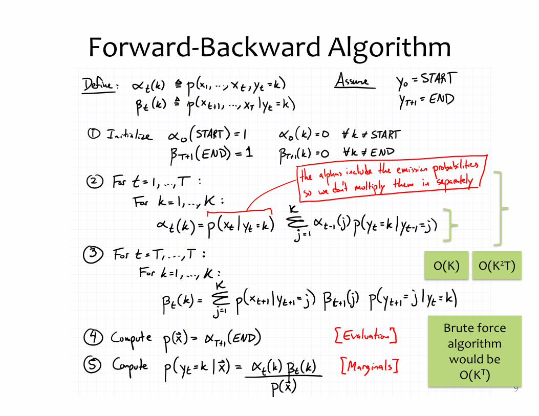
Forward-Backward Algorithm
7
O(K) O(K2T)
Brute force algorithm would be
O(KT)
Inference for HMMs
Whiteboard– Forward-backward algorithm
(edge weights version)– Viterbi algorithm
(edge weights version)
8
Forward-Backward Algorithm
9
O(K) O(K2T)
Brute force algorithm would be
O(KT)
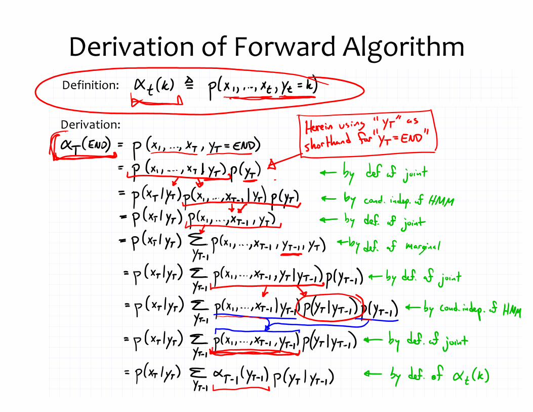
Derivation of Forward Algorithm
10
Derivation:
Definition:

Viterbi Algorithm
11

Inference in HMMsWhat is the computational complexity of inference for HMMs?
• The naïve (brute force) computations for Evaluation, Decoding, and Marginals take exponential time, O(KT)
• The forward-backward algorithm and Viterbialgorithm run in polynomial time, O(T*K2)– Thanks to dynamic programming!
12

Shortcomings of Hidden Markov Models
• HMM models capture dependences between each state and only its corresponding observation – NLP example: In a sentence segmentation task, each segmental state may depend
not just on a single word (and the adjacent segmental stages), but also on the (non-local) features of the whole line such as line length, indentation, amount of white space, etc.
• Mismatch between learning objective function and prediction objective function– HMM learns a joint distribution of states and observations P(Y, X), but in a prediction
task, we need the conditional probability P(Y|X)
© Eric Xing @ CMU, 2005-2015 13
Y1 Y2 … … … Yn
X1 X2 … … … Xn
START

MBR DECODING
14

Inference for HMMs
– Three Inference Problems for an HMM1. Evaluation: Compute the probability of a given
sequence of observations
2. Viterbi Decoding: Find the most-likely sequence of hidden states, given a sequence of observations
3. Marginals: Compute the marginal distribution for a hidden state, given a sequence of observations
4. MBR Decoding: Find the lowest loss sequence of hidden states, given a sequence of observations (Viterbi decoding is a special case)
15
Four

Minimum Bayes Risk Decoding• Suppose we given a loss function l(y’, y) and are
asked for a single tagging• How should we choose just one from our probability
distribution p(y|x)?• A minimum Bayes risk (MBR) decoder h(x) returns
the variable assignment with minimum expected loss under the model’s distribution
16
h✓(x) = argminy
Ey⇠p✓(·|x)[`(y,y)]
= argminy
X
y
p✓(y | x)`(y,y)

The 0-1 loss function returns 1 only if the two assignments are identical and 0 otherwise:
The MBR decoder is:
which is exactly the Viterbi decoding problem!
Minimum Bayes Risk Decoding
Consider some example loss functions:
17
`(y,y) = 1� I(y,y)
h✓(x) = argminy
X
y
p✓(y | x)(1� I(y,y))
= argmaxy
p✓(y | x)
h✓(x) = argminy
Ey⇠p✓(·|x)[`(y,y)]
= argminy
X
y
p✓(y | x)`(y,y)

The Hamming loss corresponds to accuracy and returns the number of incorrect variable assignments:
The MBR decoder is:
This decomposes across variables and requires the variable marginals.
Minimum Bayes Risk Decoding
Consider some example loss functions:
18
`(y,y) =VX
i=1
(1� I(yi, yi))
yi = h✓(x)i = argmaxyi
p✓(yi | x)
h✓(x) = argminy
Ey⇠p✓(·|x)[`(y,y)]
= argminy
X
y
p✓(y | x)`(y,y)

Learning ObjectivesHidden Markov Models
You should be able to…1. Show that structured prediction problems yield high-computation inference
problems2. Define the first order Markov assumption3. Draw a Finite State Machine depicting a first order Markov assumption4. Derive the MLE parameters of an HMM5. Define the three key problems for an HMM: evaluation, decoding, and
marginal computation
6. Derive a dynamic programming algorithm for computing the marginal probabilities of an HMM
7. Interpret the forward-backward algorithm as a message passing algorithm8. Implement supervised learning for an HMM9. Implement the forward-backward algorithm for an HMM10. Implement the Viterbi algorithm for an HMM
11. Implement a minimum Bayes risk decoder with Hamming loss for an HMM
19
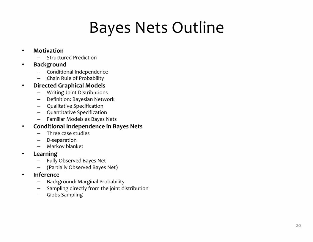
Bayes Nets Outline
• Motivation– Structured Prediction
• Background– Conditional Independence– Chain Rule of Probability
• Directed Graphical Models– Writing Joint Distributions
– Definition: Bayesian Network
– Qualitative Specification– Quantitative Specification
– Familiar Models as Bayes Nets
• Conditional Independence in Bayes Nets– Three case studies
– D-separation– Markov blanket
• Learning– Fully Observed Bayes Net
– (Partially Observed Bayes Net)
• Inference– Background: Marginal Probability
– Sampling directly from the joint distribution– Gibbs Sampling
20

DIRECTED GRAPHICAL MODELSBayesian Networks
21

Example: Ryan Reynolds’ Voicemail
22From https://www.adweek.com/brand-marketing/ryan-reynolds-left-voicemails-for-all-mint-mobile-subscribers/

Example: Ryan Reynolds Voicemail
23Images from imdb.com

Example: Ryan Reynolds’ Voicemail
24From https://www.adweek.com/brand-marketing/ryan-reynolds-left-voicemails-for-all-mint-mobile-subscribers/

Directed Graphical Models (Bayes Nets)
Whiteboard– Example: Ryan Reynolds’ Voicemail
– Writing Joint Distributions• Idea #1: Giant Table
• Idea #2: Rewrite using chain rule
• Idea #3: Assume full independence
• Idea #4: Drop variables from RHS of conditionals
– Definition: Bayesian Network
25
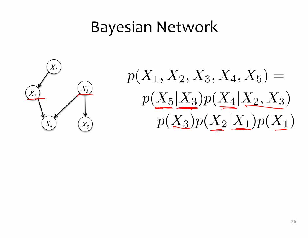
Bayesian Network
26
p(X1, X2, X3, X4, X5) =
p(X5|X3)p(X4|X2, X3)
p(X3)p(X2|X1)p(X1)
X1
X3X2
X4 X5
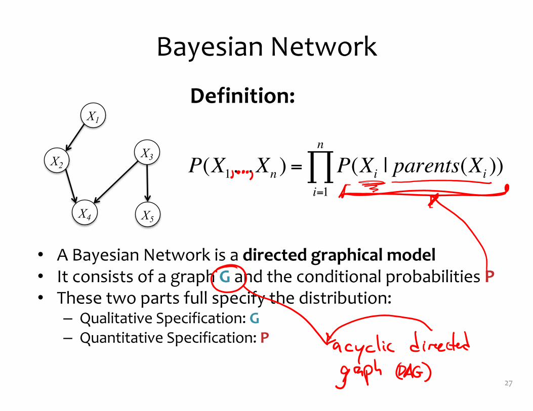
Bayesian Network
• A Bayesian Network is a directed graphical model• It consists of a graph G and the conditional probabilities P• These two parts full specify the distribution:
– Qualitative Specification: G– Quantitative Specification: P
27
X1
X3X2
X4 X5
Definition:
P(X1…Xn ) = P(Xi | parents(Xi ))i=1
n
∏

Qualitative Specification
• Where does the qualitative specification come from?
– Prior knowledge of causal relationships
– Prior knowledge of modular relationships
– Assessment from experts
– Learning from data (i.e. structure learning)
– We simply prefer a certain architecture (e.g. a layered graph)
– …
© Eric Xing @ CMU, 2006-2011 28

a0 0.75a1 0.25
b0 0.33b1 0.67
a0b0 a0b1 a1b0 a1b1
c0 0.45 1 0.9 0.7c1 0.55 0 0.1 0.3
A B
C
P(a,b,c.d) =
P(a)P(b)P(c|a,b)P(d|c)
D
c0 c1
d0 0.3 0.5d1 07 0.5
Quantitative Specification
29© Eric Xing @ CMU, 2006-2011
Example: Conditional probability tables (CPTs)for discrete random variables
A B
C
P(a,b,c.d) = P(a)P(b)P(c|a,b)P(d|c)
D
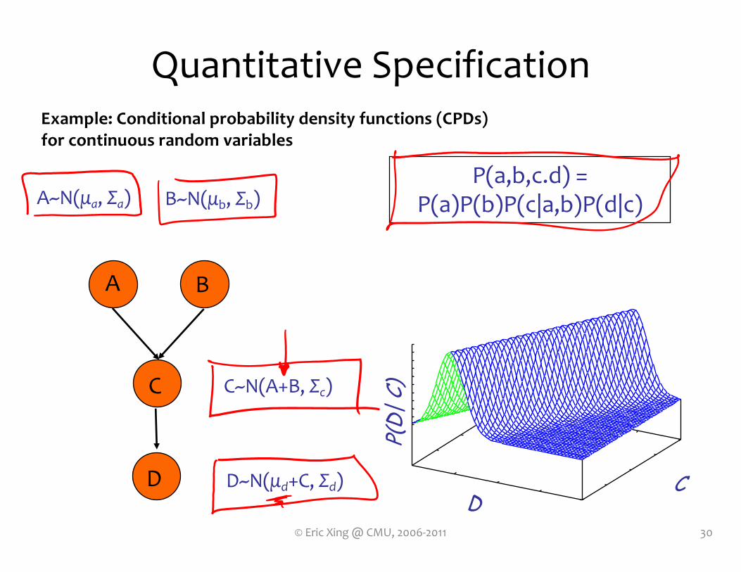
A~N(μa, Σa) B~N(μb, Σb)
C~N(A+B, Σc)
D~N(μd+C, Σd)D
C
P(D|
C)
Quantitative Specification
30© Eric Xing @ CMU, 2006-2011
Example: Conditional probability density functions (CPDs)for continuous random variables

A B
C
P(a,b,c.d) = P(a)P(b)P(c|a,b)P(d|c)
D
C~N(A+B, Σc)
D~N(μd+C, Σd)
Quantitative Specification
31© Eric Xing @ CMU, 2006-2011
Example: Combination of CPTs and CPDs for a mix of discrete and continuous variables
a0 0.75a1 0.25
b0 0.33b1 0.67
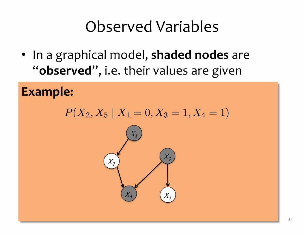
Example:
Observed Variables
• In a graphical model, shaded nodes are “observed”, i.e. their values are given
32
X1
X3X2
X4 X5

Familiar Models as Bayesian Networks
33
Question:Match the model name to the corresponding Bayesian Network1. Logistic Regression2. Linear Regression3. Bernoulli Naïve Bayes4. Gaussian Naïve Bayes5. 1D Gaussian
Answer:Y
XMX1 X2 …
Y
XMX1 X2 …
Y
XMX1 X2 …
Y
XMX1 X2 …
X
µ σ2
X
A B
C D
E F