machine%learning%department …mgormley/courses/10601-s17/...regression%vs.%collaborative%filtering...
TRANSCRIPT
Matrix Factorizationand
Collaborative Filtering
1
10-‐601 Introduction to Machine Learning
Matt GormleyLecture 25
April 19, 2017
Machine Learning DepartmentSchool of Computer ScienceCarnegie Mellon University
MF Readings:(Koren et al., 2009)
Reminders
• Homework 8: Graphical Models– Release: Mon, Apr. 17– Due: Mon, Apr. 24 at 11:59pm
• Homework 9: Applications of ML– Release: Mon, Apr. 24– Due: Wed, May 3 at 11:59pm
2
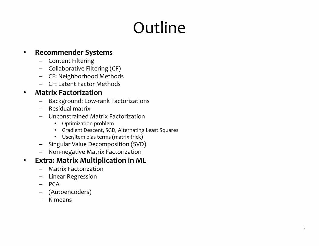
Outline• Recommender Systems
– Content Filtering– Collaborative Filtering (CF)– CF: Neighborhood Methods– CF: Latent Factor Methods
• Matrix Factorization– Background: Low-‐rank Factorizations– Residual matrix– Unconstrained Matrix Factorization
• Optimization problem• Gradient Descent, SGD, Alternating Least Squares• User/item bias terms (matrix trick)
– Singular Value Decomposition (SVD)– Non-‐negative Matrix Factorization
• Extra: Matrix Multiplication in ML– Matrix Factorization– Linear Regression– PCA– (Autoencoders)– K-‐means
7

RECOMMENDER SYSTEMS
8
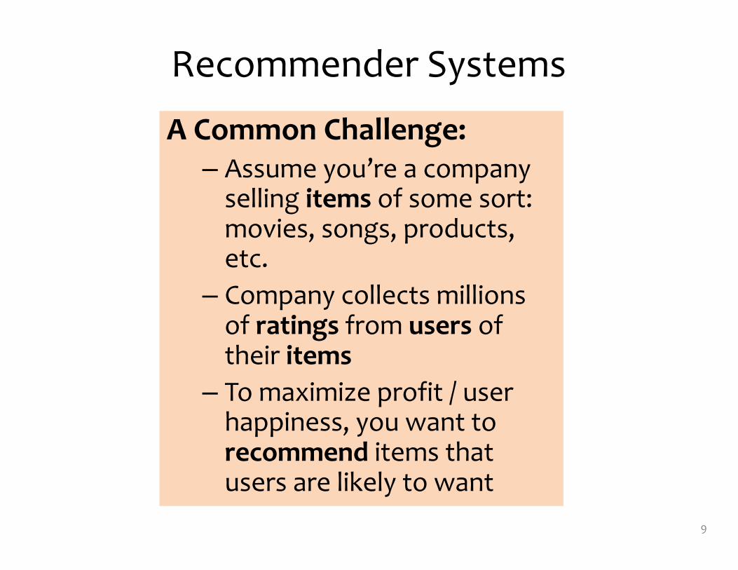
Recommender Systems
A Common Challenge:– Assume you’re a company selling items of some sort: movies, songs, products, etc.
– Company collects millions of ratings from users of their items
– To maximize profit / user happiness, you want to recommend items that users are likely to want
9

Recommender Systems
10
Recommender Systems
11

Recommender Systems
12
Recommender Systems
13
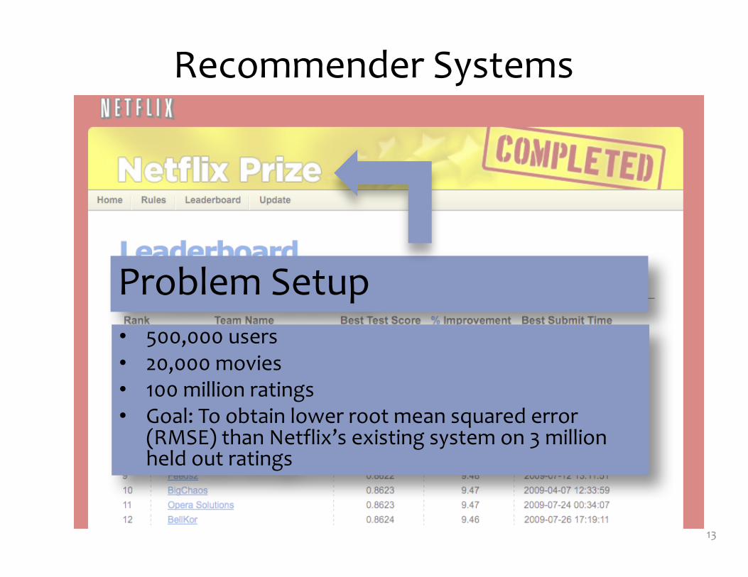
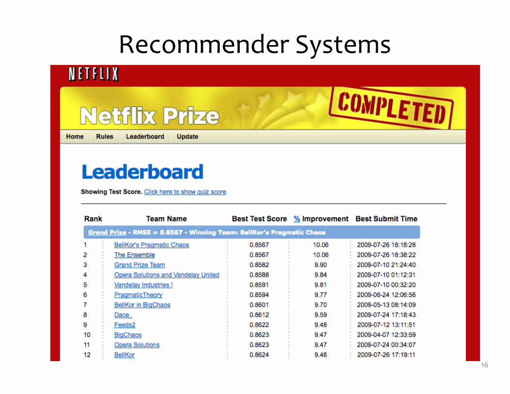
Problem Setup• 500,000 users• 20,000 movies• 100 million ratings• Goal: To obtain lower root mean squared error
(RMSE) than Netflix’s existing system on 3 million held out ratings
Recommender Systems
14
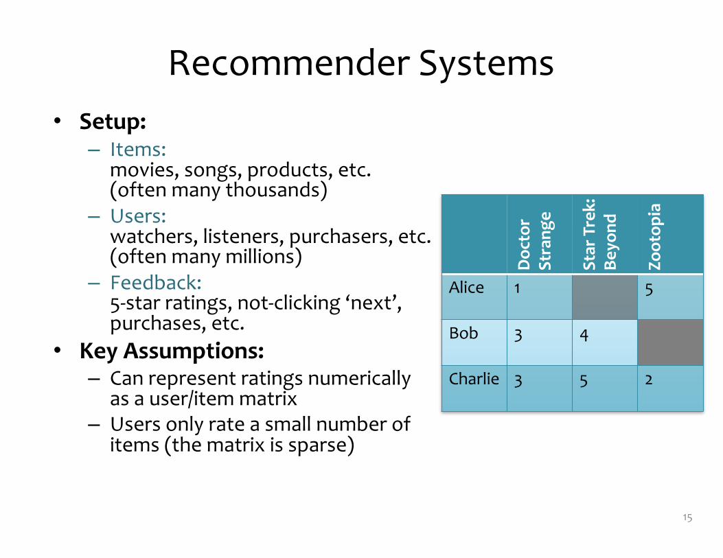
Recommender Systems• Setup:
– Items: movies, songs, products, etc.(often many thousands)
– Users: watchers, listeners, purchasers, etc.(often many millions)
– Feedback: 5-‐star ratings, not-‐clicking ‘next’, purchases, etc.
• Key Assumptions:– Can represent ratings numerically
as a user/item matrix– Users only rate a small number of
items (the matrix is sparse)
15Doc
tor
Strang
e
Star Trek:
Beyo
nd
Zootop
ia
Alice 1 5
Bob 3 4
Charlie 3 5 2
Recommender Systems
16
Two Types of Recommender Systems
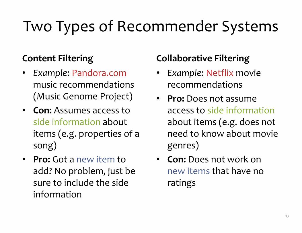
Content Filtering• Example: Pandora.com
music recommendations (Music Genome Project)
• Con: Assumes access to side information about items (e.g. properties of a song)
• Pro: Got a new item to add? No problem, just be sure to include the side information
Collaborative Filtering• Example: Netflix movie
recommendations• Pro: Does not assume
access to side information about items (e.g. does not need to know about movie genres)
• Con: Does not work on new items that have no ratings
17

COLLABORATIVE FILTERING
19
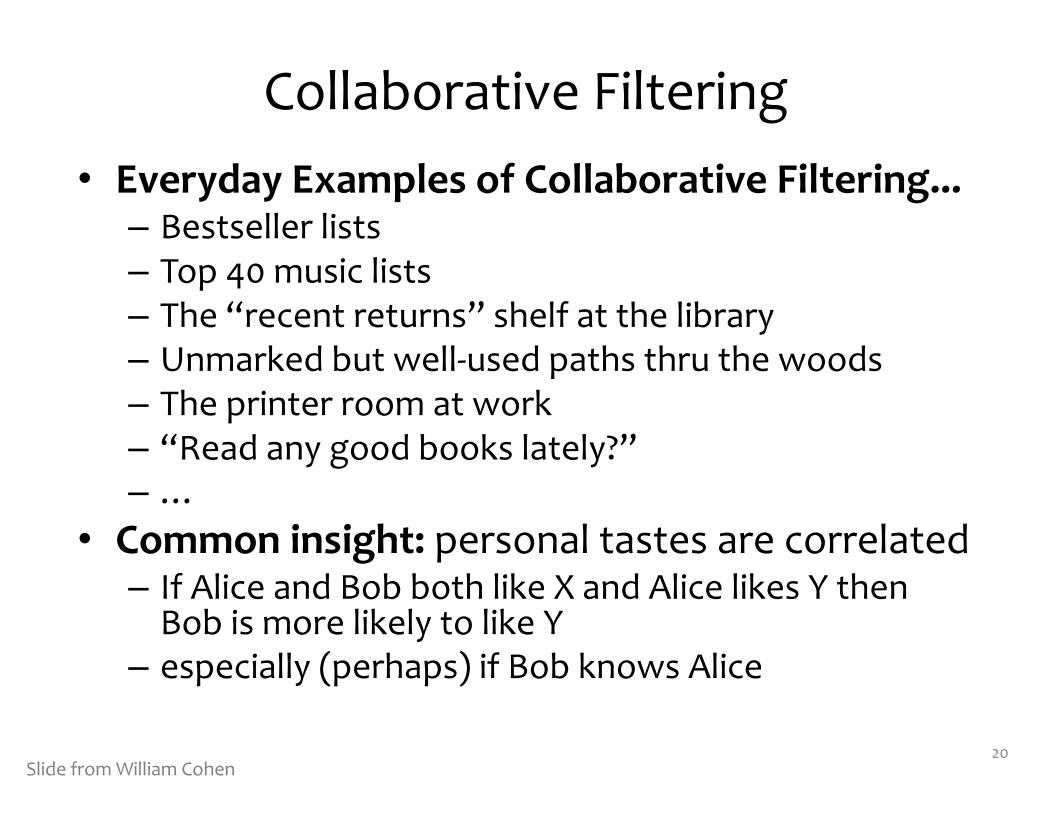
Collaborative Filtering• Everyday Examples of Collaborative Filtering...– Bestseller lists– Top 40 music lists– The “recent returns” shelf at the library– Unmarked but well-‐used paths thru the woods– The printer room at work– “Read any good books lately?”– …
• Common insight: personal tastes are correlated– If Alice and Bob both like X and Alice likes Y then Bob is more likely to like Y
– especially (perhaps) if Bob knows Alice
20Slide from William Cohen
Two Types of Collaborative Filtering
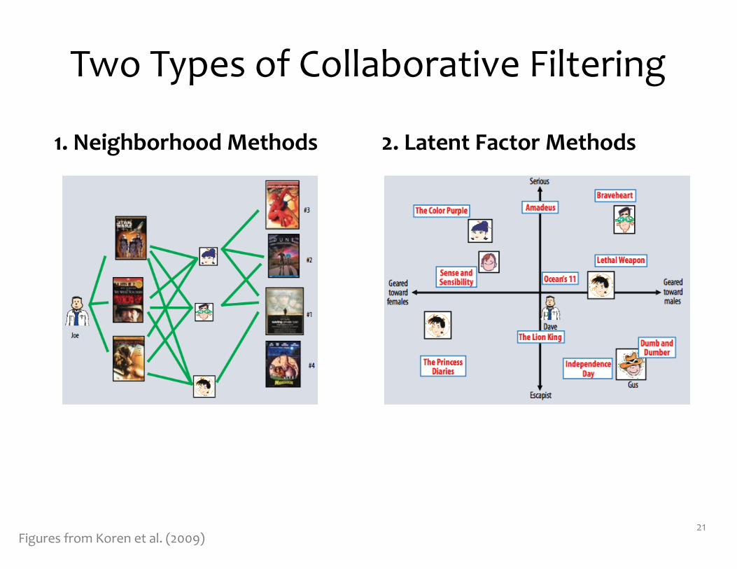
1. Neighborhood Methods 2. Latent Factor Methods
21Figures from Koren et al. (2009)
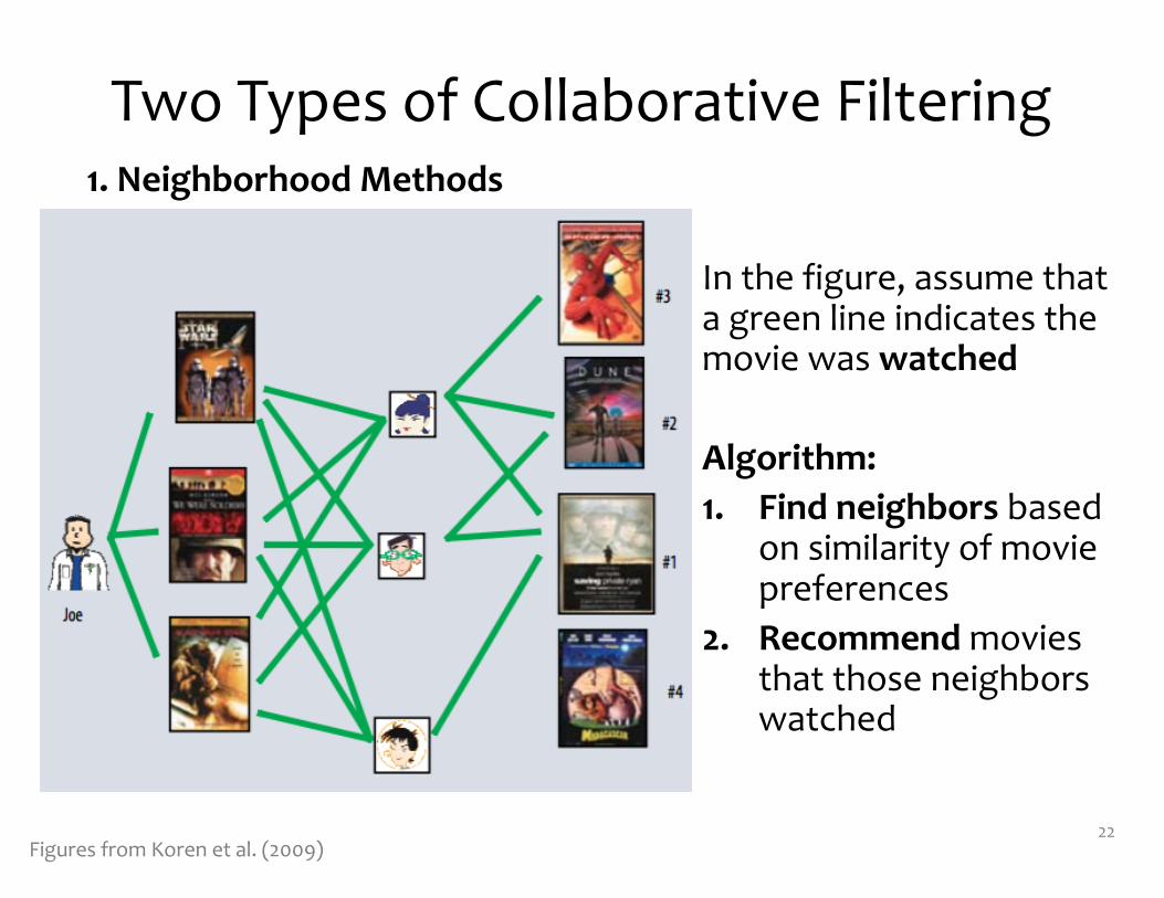
Two Types of Collaborative Filtering1. Neighborhood Methods
22
In the figure, assume that a green line indicates the movie was watched
Algorithm:1. Find neighbors based
on similarity of movie preferences
2. Recommendmovies that those neighbors watched
Figures from Koren et al. (2009)
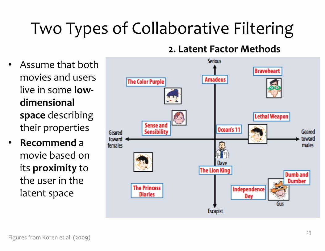
Two Types of Collaborative Filtering2. Latent Factor Methods
23Figures from Koren et al. (2009)
• Assume that both movies and users live in some low-‐dimensional space describing their properties
• Recommend a movie based on its proximity to the user in the latent space

MATRIX FACTORIZATION
24
Matrix Factorization
• Many different ways of factorizing a matrix• We’ll consider three:
1. Unconstrained Matrix Factorization2. Singular Value Decomposition3. Non-‐negative Matrix Factorization
• MF is just another example of a common recipe:
1. define a model2. define an objective function3. optimize with SGD
25
Matrix Factorization
Whiteboard– Background: Low-‐rank Factorizations– Residual matrix
27
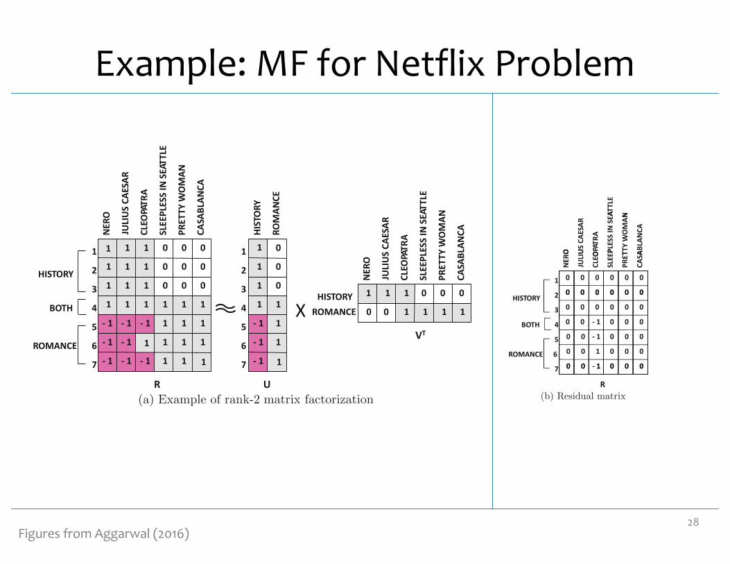
Example: MF for Netflix Problem
28Figures from Aggarwal (2016)
3.6. LATENT FACTOR MODELS 95
1
2
3
4
5
6
7
HIST
ORY
ROM
ANCE
X HISTORY
ROMANCE
ROMANCE
BOTH
HISTORY
1 1 1
1 1 1
1 1 1
- 1
- 1
- 1
- 1
- 1
- 1 - 1 - 1
1 1 1 1 1 1
1 1 1
1 1 1 1
1 1 1
0 0 0
0 0 0
0 0 0
NERO
JULI
US C
AESA
R
CLEO
PATR
A
SLEE
PLES
S IN
SEA
TTLE
PRET
TY W
OM
AN
CASA
BLAN
CA
R U
VT
NERO
JULI
US C
AESA
R
CLEO
PATR
A
SLEE
PLES
S IN
SEA
TTLE
PRET
TY W
OM
AN
CASA
BLAN
CA
0
0
0
- 1
- 1
- 1
1
1
1
1
1
1
1
1 1 1 1
1 1 1 1 0 0
0 0 0
6
7
5
4
3
2
1
ATTL
E
N
O USCA
ESAR
OPA
TRA
PLES
SIN
SEA
T TY
WO
MAN
ABLA
NCA
0 0 0
0 0 0
0 0 0
0 0 0
NERO
JULI
U
CLEO
SLEE
P
PRET
CASA
1
BOTH
HISTORY0 0 0
0 0 0
0 0 0 0 0
0 0 0
0 0 0
1
2
3
4
ROMANCE
0
0
0
0
0 0
1
0 0 0
1
0 0 0
0 0 0
15
60 0 1 0 0 0
R
7
(a) Example of rank-2 matrix factorization
(b) Residual matrix
Figure 3.7: Example of a matrix factorization and its residual matrix
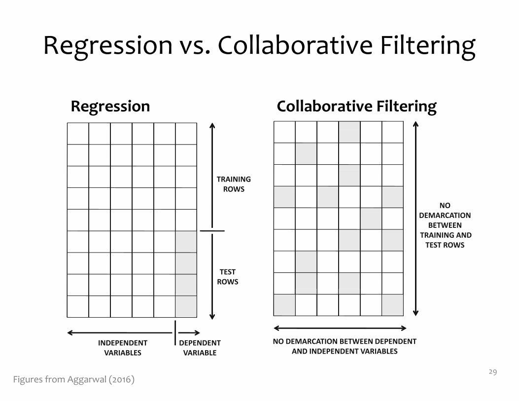
Regression vs. Collaborative Filtering
29
72 CHAPTER 3. MODEL-BASED COLLABORATIVE FILTERING
TRAININGROWS
TESTROWS
INDEPENDENTVARIABLES
DEPENDENTVARIABLE
NODEMARCATION
BETWEENTRAINING ANDTEST ROWS
NO DEMARCATION BETWEEN DEPENDENTAND INDEPENDENT VARIABLES
(a) Classification (b) Collaborative filtering
Figure 3.1: Revisiting Figure 1.4 of Chapter 1. Comparing the traditional classificationproblem with collaborative filtering. Shaded entries are missing and need to be predicted.
the class variable (or dependent variable). All entries in the first (n− 1) columns are fullyspecified, whereas only a subset of the entries in the nth column is specified. Therefore, asubset of the rows in the matrix is fully specified, and these rows are referred to as thetraining data. The remaining rows are referred to as the test data. The values of the missingentries need to be learned for the test data. This scenario is illustrated in Figure 3.1(a),where the shaded values represent missing entries in the matrix.
Unlike data classification, any entry in the ratings matrix may be missing, as illustratedby the shaded entries in Figure 3.1(b). Thus, it can be clearly seen that the matrix com-pletion problem is a generalization of the classification (or regression modeling) problem.Therefore, the crucial differences between these two problems may be summarized as follows:
1. In the data classification problem, there is a clear separation between feature (inde-pendent) variables and class (dependent) variables. In the matrix completion problem,this clear separation does not exist. Each column is both a dependent and independentvariable, depending on which entries are being considered for predictive modeling ata given point.
2. In the data classification problem, there is a clear separation between the trainingand test data. In the matrix completion problem, this clear demarcation does notexist among the rows of the matrix. At best, one can consider the specified (observed)entries to be the training data, and the unspecified (missing) entries to be the testdata.
3. In data classification, columns represent features, and rows represent data instances.However, in collaborative filtering, it is possible to apply the same approach to ei-ther the ratings matrix or to its transpose because of how the missing entries aredistributed. For example, user-based neighborhood models can be viewed as direct
Figures from Aggarwal (2016)
Regression Collaborative Filtering

UNCONSTRAINED MATRIX FACTORIZATION
30
Unconstrained Matrix Factorization
Whiteboard– Optimization problem– SGD– SGD with Regularization– Alternating Least Squares– User/item bias terms (matrix trick)
31
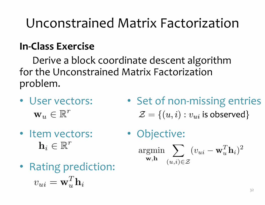
Unconstrained Matrix FactorizationIn-‐Class Exercise
Derive a block coordinate descent algorithm for the Unconstrained Matrix Factorization problem.
32
• User vectors:
• Item vectors:
• Rating prediction:
u � Rr
i � Rr
vui = Tu i
• Set of non-‐missing entries:
• Objective:
,
�
(u,i)�Z
(vui � Tu i)
2
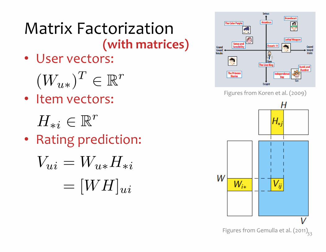
Matrix Factorization
• User vectors:
• Item vectors:
• Rating prediction:
33
Figures from Koren et al. (2009)
H�i � Rr
(Wu�)T � Rr
Matrix$factorization$as$SGD$V$why$does$this$work?$$Here’s$the$key$claim:
Figures from Gemulla et al. (2011)
Vui = Wu�H�i
= [WH]ui
(with matrices)
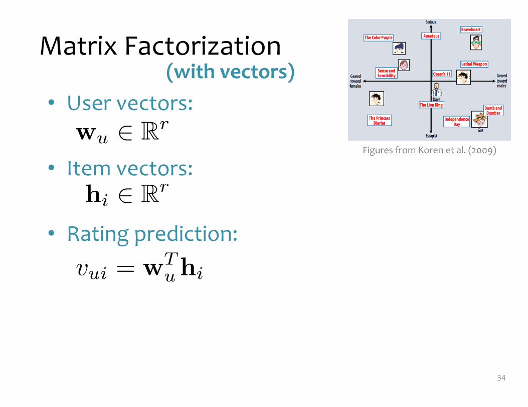
• User vectors:
• Item vectors:
• Rating prediction:
Matrix Factorization(with vectors)
34
Figures from Koren et al. (2009)u � Rr
i � Rr
vui = Tu i
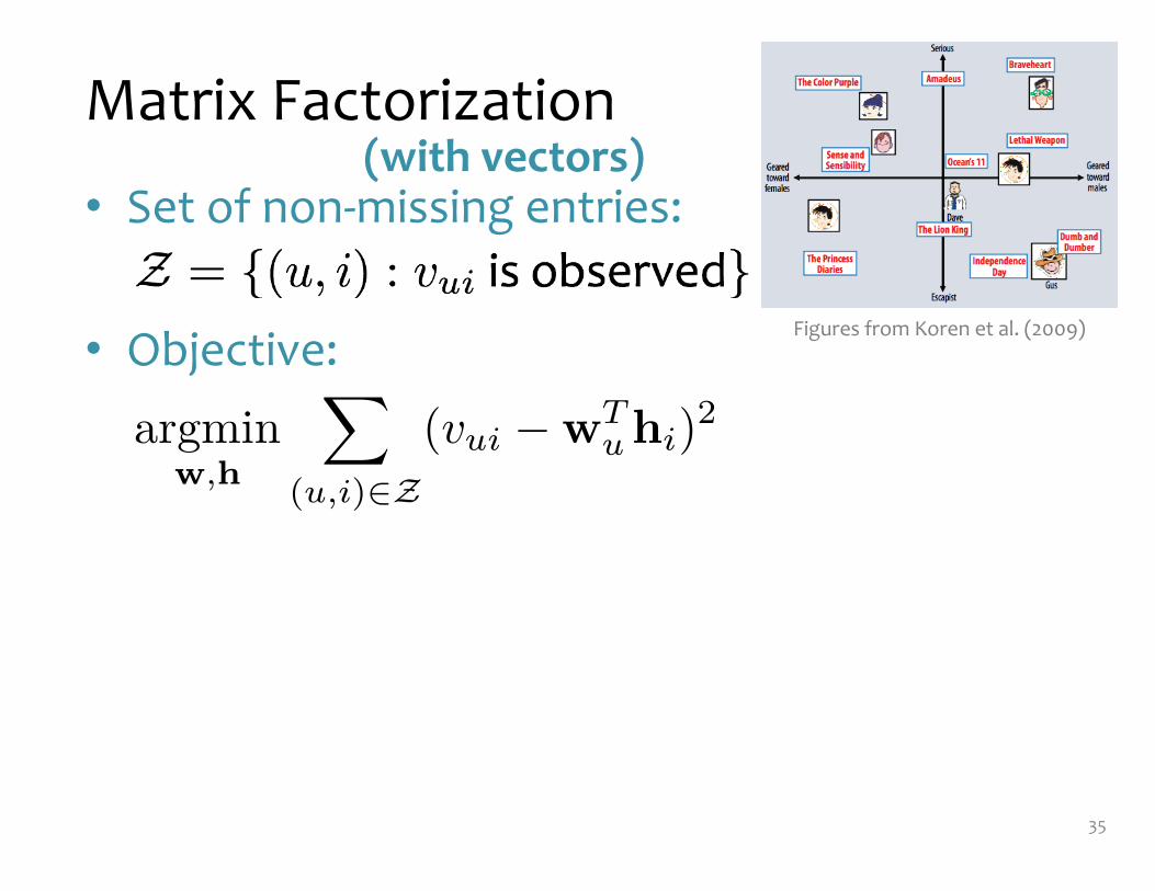
Matrix Factorization
• Set of non-‐missing entries:
• Objective:
35
Figures from Koren et al. (2009)
,
�
(u,i)�Z
(vui � Tu i)
2
(with vectors)
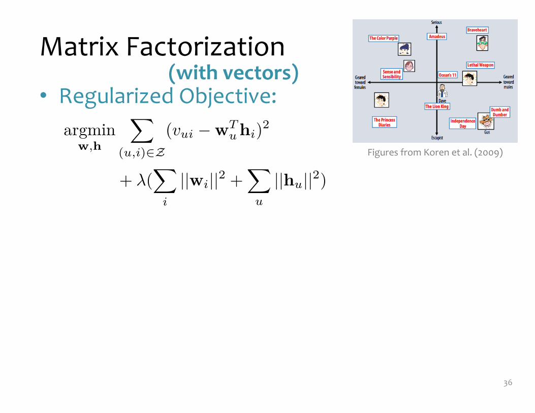
Matrix Factorization
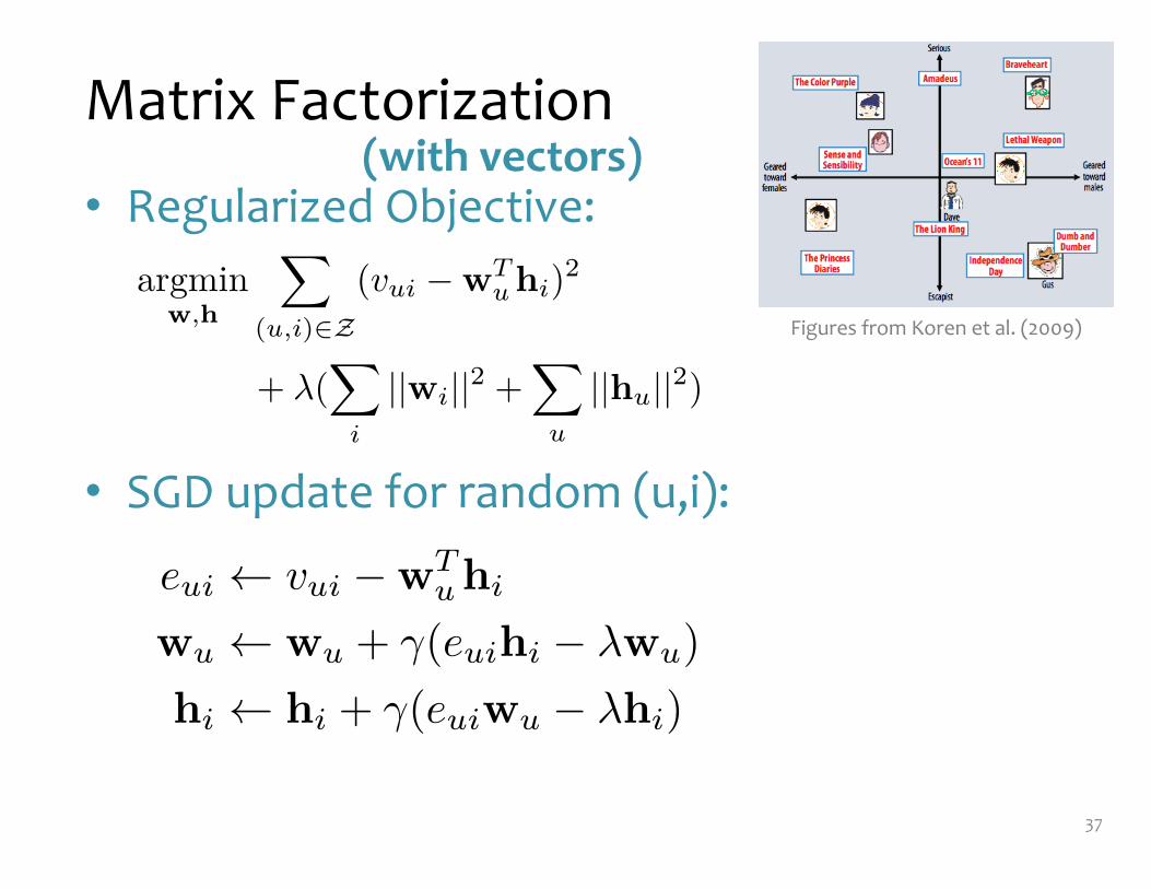
• Regularized Objective:
• SGD update for random (u,i):
36
Figures from Koren et al. (2009)
(with vectors)
,
�
(u,i)�Z
(vui � Tu i)
2
+ �(�
i
|| i||2 +�
u
|| u||2)
Matrix Factorization
• Regularized Objective:
• SGD update for random (u,i):
37
Figures from Koren et al. (2009)
(with vectors)
eui � vui � Tu i
u � u + �(eui i � � u)
i � i + �(eui u � � i)
,
�
(u,i)�Z
(vui � Tu i)
2
+ �(�
i
|| i||2 +�
u
|| u||2)

Matrix Factorization
• User vectors:
• Item vectors:
• Rating prediction:
38
Figures from Koren et al. (2009)
H�i � Rr
(Wu�)T � Rr
Matrix$factorization$as$SGD$V$why$does$this$work?$$Here’s$the$key$claim:
Figures from Gemulla et al. (2011)
Vui = Wu�H�i
= [WH]ui
(with matrices)
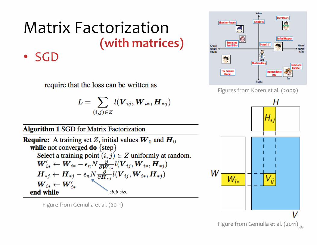
Matrix Factorization
• SGD
39
Figures from Koren et al. (2009)
Matrix$factorization$as$SGD$V$why$does$this$work?$$Here’s$the$key$claim:
Figure from Gemulla et al. (2011)
(with matrices)Matrix$factorization$as$SGD$V$why$does$
this$work?
step size
Figure from Gemulla et al. (2011)
Matrix Factorization
40
47AUGUST 2009
Our winning entries consist of more than 100 differ-ent predictor sets, the majority of which are factorization models using some variants of the methods described here. Our discussions with other top teams and postings on the public contest forum indicate that these are the most popu-lar and successful methods for predicting ratings.
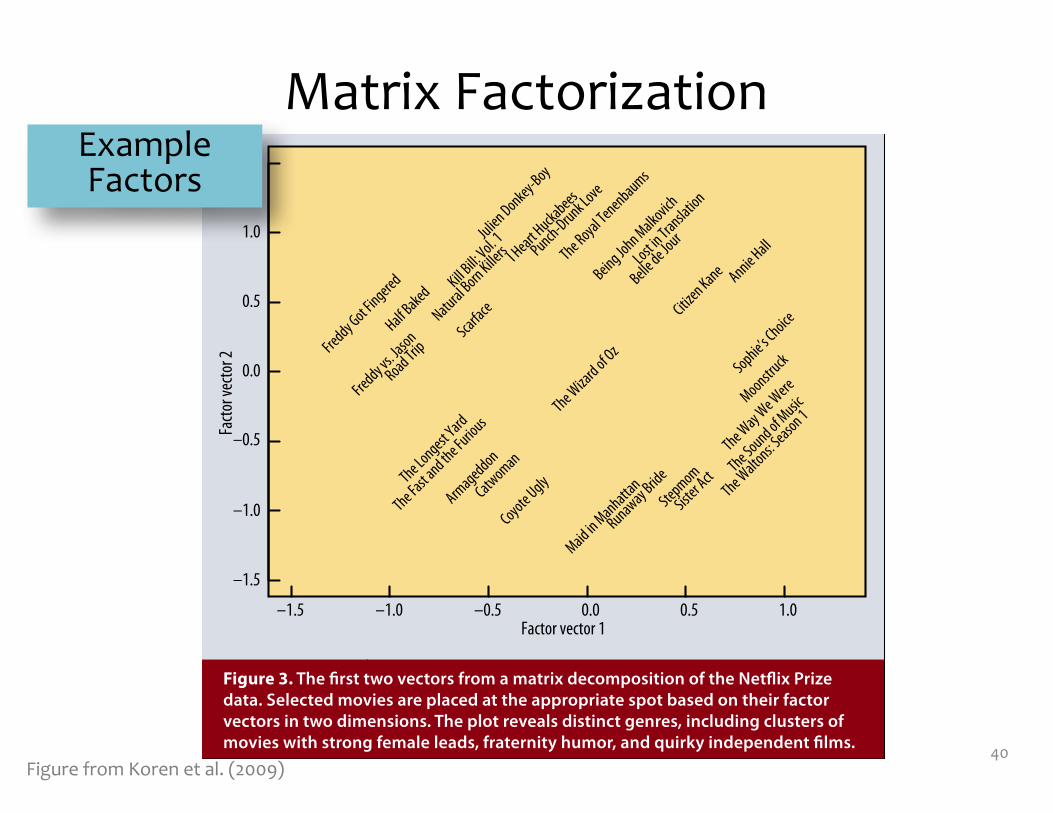
Factorizing the Netflix user-movie matrix allows us to discover the most descriptive dimensions for predict-ing movie preferences. We can identify the first few most important dimensions from a matrix decomposition and explore the movies’ location in this new space. Figure 3 shows the first two factors from the Netflix data matrix factorization. Movies are placed according to their factor vectors. Someone familiar with the movies shown can see clear meaning in the latent factors. The first factor vector (x-axis) has on one side lowbrow comedies and horror movies, aimed at a male or adolescent audience (Half Baked, Freddy vs. Jason), while the other side contains drama or comedy with serious undertones and strong female leads (Sophie’s Choice, Moonstruck). The second factorization axis (y-axis) has independent, critically acclaimed, quirky films (Punch-Drunk Love, I Heart Huckabees) on the top, and on the bottom, mainstream formulaic films (Armaged-don, Runaway Bride). There are interesting intersections between these boundaries: On the top left corner, where indie meets lowbrow, are Kill Bill and Natural Born Kill-ers, both arty movies that play off violent themes. On the bottom right, where the serious female-driven movies meet
preferences might cause a one-time event; however, a recurring event is more likely to reflect user opinion.
The matrix factorization model can readily accept varying confidence levels, which let it give less weight to less meaningful observations. If con-fidence in observing rui is denoted as cui, then the model enhances the cost function (Equation 5) to account for confidence as follows:
min* * *, ,p q b
( , )u i
cui(rui µ bu bi
puTqi)
2 + (|| pu ||2 + || qi ||
2 + bu
2 + bi2) (8)
For information on a real-life ap-plication involving such schemes, refer to “Collaborative Filtering for Implicit Feedback Datasets.”10
NETFLIX PRIZE COMPETITION
In 2006, the online DVD rental company Netflix announced a con-test to improve the state of its recommender system.12 To enable this, the company released a training set of more than 100 million ratings spanning about 500,000 anony-mous customers and their ratings on more than 17,000 movies, each movie being rated on a scale of 1 to 5 stars. Participating teams submit predicted ratings for a test set of approximately 3 million ratings, and Netflix calculates a root-mean -square error (RMSE) based on the held-out truth. The first team that can improve on the Netflix algo-rithm’s RMSE performance by 10 percent or more wins a $1 million prize. If no team reaches the 10 percent goal, Netflix gives a $50,000 Progress Prize to the team in first place after each year of the competition.
The contest created a buzz within the collaborative fil-tering field. Until this point, the only publicly available data for collaborative filtering research was orders of magni-tude smaller. The release of this data and the competition’s allure spurred a burst of energy and activity. According to the contest website (www.netflixprize.com), more than 48,000 teams from 182 different countries have down-loaded the data.
Our team’s entry, originally called BellKor, took over the top spot in the competition in the summer of 2007, and won the 2007 Progress Prize with the best score at the time: 8.43 percent better than Netflix. Later, we aligned with team Big Chaos to win the 2008 Progress Prize with a score of 9.46 percent. At the time of this writing, we are still in first place, inching toward the 10 percent landmark.
–1.5 –1.0 –0.5 0.0 0.5 1.0
–1.5
–1.0
–0.5
0.0
0.5
1.0
1.5
Factor vector 1
Facto
r vec
tor 2
Freddy Got Fingered
Freddy vs. Jason
Half Baked
Road Trip
The Sound of Music
Sophie’s Choice
Moonstruck
Maid in Manhattan
The Way We Were
Runaway Bride
Coyote Ugly
The Royal Tenenbaums
Punch-Drunk Love
I Heart Huckabees
Armageddon
Citizen Kane
The Waltons: Season 1
Stepmom
Julien Donkey-Boy
Sister Act
The Fast and the Furious
The Wizard of Oz
Kill Bill:
Vol. 1
ScarfaceNatural Born Killers
Annie Hall
Belle de JourLost i
n Translation
The Longest Yard
Being John Malkovich
Catwoman
Figure 3. The first two vectors from a matrix decomposition of the Netflix Prize data. Selected movies are placed at the appropriate spot based on their factor vectors in two dimensions. The plot reveals distinct genres, including clusters of movies with strong female leads, fraternity humor, and quirky independent films.
Figure from Koren et al. (2009)
Example Factors
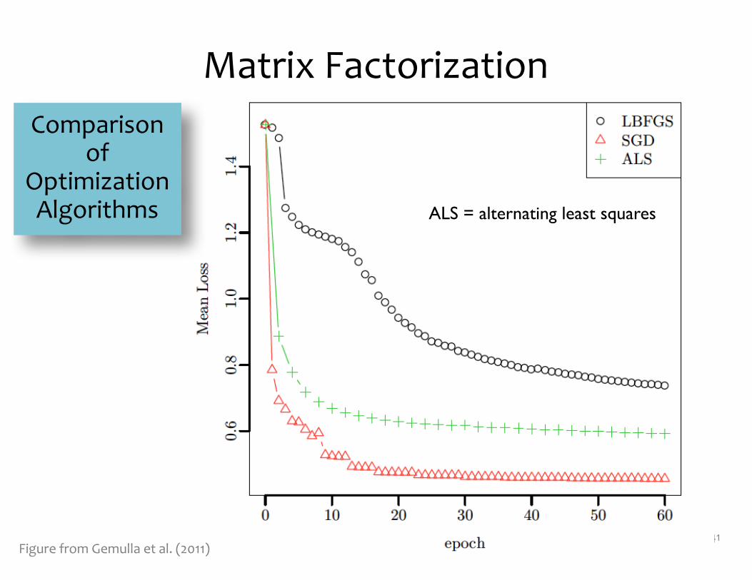
Matrix Factorization
41
ALS = alternating least squares
Comparison of
Optimization Algorithms
Figure from Gemulla et al. (2011)

SVD FOR COLLABORATIVE FILTERING
42
Singular Value Decompositionfor Collaborative Filtering
Whiteboard– Optimization problem– Equivalence to Unconstrained Matrix Factorization (fully specified, no regularization)
43
NON-‐NEGATIVE MATRIX FACTORIZATION
44
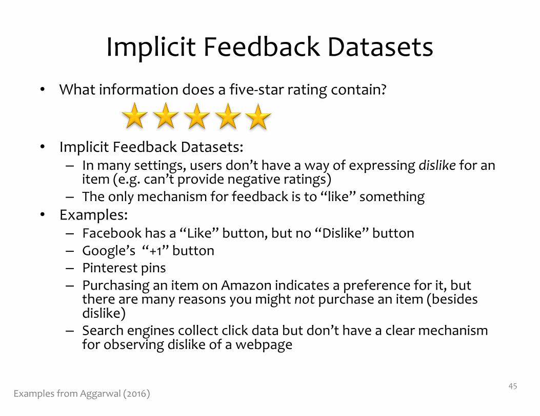
Implicit Feedback Datasets• What information does a five-‐star rating contain?
• Implicit Feedback Datasets:– In many settings, users don’t have a way of expressing dislike for an
item (e.g. can’t provide negative ratings)– The only mechanism for feedback is to “like” something
• Examples:– Facebook has a “Like” button, but no “Dislike” button– Google’s “+1” button– Pinterest pins– Purchasing an item on Amazon indicates a preference for it, but
there are many reasons you might not purchase an item (besides dislike)
– Search engines collect click data but don’t have a clear mechanism for observing dislike of a webpage
45Examples from Aggarwal (2016)
Non-‐negative Matrix Factorization
Whiteboard– Optimization problem–Multiplicative updates
46
Summary
• Recommender systems solve many real-‐world (*large-‐scale) problems
• Collaborative filtering by Matrix Factorization (MF) is an efficient and effective approach
• MF is just another example of a common recipe:
1. define a model2. define an objective function3. optimize with SGD
55