Low-Frequency Robust Cointegration Testing�

Ulrich K. Müller

Princeton University

Department of Economics

Princeton, NJ, 08544

Mark W. Watson

Princeton University

Department of Economics

and Woodrow Wilson School

Princeton, NJ, 08544

June 2007(This version: February 2013)

Abstract

Standard inference in cointegrating models is fragile because it relies on an assump-

tion of an I(1) model for the common stochastic trends, which may not accurately

describe the data�s persistence. This paper considers low-frequency tests about coin-

tegrating vectors under a range of restrictions on the common stochastic trends. We

quantify how much power can potentially be gained by exploiting correct restrictions,

as well as the magnitude of size distortions if such restrictions are imposed erroneously.

A simple test motivated by the analysis in Wright (2000) is developed and shown to

be approximately optimal for inference about a single cointegrating vector in the un-

restricted stochastic trend model.

JEL classi�cation: C32, C12

Keywords: stochastic trends, persistence, size distortion, interest rates, term

spread

�We thank participants of the Cowles Econometrics Conference, the NBER Summer Institute and the

Greater New York Metropolitan Area Econometrics Colloquium, and of seminars at Chicago, Cornell, North-

western, NYU, Rutgers, and UCSD for helpful discussions. Support was provided by the National Science

Foundation through grants SES-0518036 and SES-0617811.

1 Introduction

The fundamental insight of cointegration is that while economic time series may be individ-

ually highly persistent, some linear combinations are much less persistent. Accordingly, a

suite of practical methods have been developed for conducting inference about cointegrat-

ing vectors, the coe¢ cients that lead to this reduction in persistence. In their standard

form, these methods assume that the persistence is the result of common I(1) stochastic

trends,1 and their statistical properties crucially depend on particular characteristics of I(1)

processes. But in many applications there is uncertainty about the correct model for the per-

sistence which cannot be resolved by examination of the data, rendering standard inference

potentially fragile. This paper studies e¢ cient inference methods for cointegrating vectors

that is robust to this fragility.

We do this using a transformation of the data that focuses on low-frequency variability

and covariability. This transformation has two distinct advantages. First, as we have ar-

gued elsewhere (Müller and Watson (2008)), persistence (�trending behavior�) and lack of

persistence (�non-trending, I(0) behavior�) are low-frequency characteristics, and attempts

to utilize high-frequency variability to learn about low-frequency variability are fraught with

their own fragilities.2 Low-frequency transformations eliminate these fragilities by focusing

attention on the features of the data that are of direct interest for questions relating to

persistence. In particular, as in Müller and Watson (2008), we suggest focussing on below

business cycle frequencies, so that the implied de�nition of cointegration is that error cor-

rection terms have a �at spectrum below business cycle frequencies. The second advantage

is an important by-product of discarding high frequency variability. The major technical

challenge when conducting robust inference about cointegrating vectors is to control size

over the range of plausible processes characterizing the model�s stochastic common trends.

Restricting attention to low frequencies greatly reduces the dimensionality of this challenge.

The potential impact of non-I(1) stochastic trends on standard cointegration inference

has long been recognized. Elliott (1998) provides a dramatic demonstration of the fragility of

standard cointegration methods by showing that they fail to control size when the common

stochastic trends are not I(1), but rather are �local-to-unity� in the sense of Bobkoski

1See, for instance, Johansen (1988), Phillips and Hansen (1990), Saikkonen (1991), Park (1992) and Stock

and Watson (1993).2Perhaps the most well-known example of this fragility involves estimation of HAC standard errors, see

Newey and West (1987), Andrews (1991), den Haan and Levin (1997), Kiefer, Vogelsang, and Bunzel (2000),

Kiefer and Vogelsang (2005), Müller (2007) and Sun, Phillips, and Jin (2008).

1

(1983), Cavanagh (1985), Chan and Wei (1987) and Phillips (1987).3 In a bivariate model,

Cavanagh, Elliott, and Stock (1995) propose several procedures to adjust critical values

from standard tests to control size over a range of values of the local-to-unity parameter,

and their general approach has been used by several other researchers; Campbell and Yogo

(2006) provides a recent example. Stock and Watson (1996), Jansson and Moreira (2006)

and Elliott, Müller, and Watson (2012) go further and develop inference procedures with

speci�c optimality properties in the local-to-unity model.

An alternative generalization of the I(0) and I(1) dichotomy is based on the fractionally

integrated model I(d), where d is not restricted to take on integer values (see, for instance,

Baillie (1996) or Robinson (2003) for introductions). Fractional cointegration is then de-

�ned by the existence of a linear combination that leads to a reduction of the fractional

parameter. A well-developed literature has studied inference in this framework: see, for in-

stance, Velasco (2003), Robinson and Marinucci (2001, 2003), Robinson and Hualde (2003)

and Chen and Hurvich (2003a, 2003b, 2006). As in the local-to-unity embedding, however,

the low-frequency variability of the common stochastic trends is still governed by a single

parameter, since (suitably scaled) partial sums of a fractionally integrated series converge

to fractional Brownian motions, which are only indexed d. In contrast to the local-to-unity

framework, this decisive parameter can be consistently estimated, so that the uncertainty

about the exact nature of the stochastic trend vanishes in this fractional framework, at least

under the usual asymptotics.

Yet, Müller and Watson (2008) demonstrate that relying on below business cycle varia-

tion, it is a hopeless endeavor to try to consistently discriminate between, say, local-to-unity

and fractionally integrated stochastic data spanning 50 years. Similarly, Clive Granger dis-

cusses a wide range of possible data generating processes beyond the I(1) model in his Frank

Paish Lecture (1993) and argues, sensibly in our opinion, that it is fruitless to attempt to

identify the exact nature of the persistence using the limited information in typical macro

time series. While local-to-unity and fractional processes generalize the assumption of I(1)

trends, they do so in a very speci�c way, leading to worries about the potential fragility of

these methods to alternative speci�cations of the stochastic trend.

As demonstrated by Wright (2000), it is nevertheless possible to conduct inference about

a cointegrating vector without knowledge about the precise nature of the common stochastic

trends. Wright�s idea is to use the I(0) property of the error correction term as the identifying

property of the true cointegrating vector, so that a stationarity test of the model�s putative

3Also see Elliott and Stock (1994) and Jeganathan (1997).

2

error correction term is used to conduct inference about the value of the cointegrating vec-

tors. Because the common stochastic trends drop out under the null hypothesis, Wright�s

procedure is robust in the sense that it controls size under any model for the common sto-

chastic trend. But the procedure ignores the data beyond the putative error correction term,

and is thus potentially quite ine¢ cient.

Section 2 of this paper provides a formulation of the cointegrated model in which the

common stochastic trends follow a �exible limiting Gaussian process that includes the I(1),

local-to-unity, and fractional/long-memory models as special cases. Section 3 discusses the

low-frequency transformation of the cointegrated model. Throughout the paper, inference

procedures are studied in the context of this general formulation of the cointegrated model.

The price to pay for this generality is that it introduces a potentially large number of nuisance

parameters that characterize the properties of the stochastic trends and the relationship

between the stochastic trends and the model�s I(0) components. In our framework, none of

these nuisance parameters can be estimated consistently. The main challenge of this paper is

thus to study e¢ cient tests in the presence of nuisance parameters under the null hypothesis,

and Sections 4�6 address this issue.

Using this framework, the paper then makes six contributions. The �rst is derive lower

bounds on size distortions associated with trend speci�cations that are more general than

those maintained under a test�s null hypothesis. For example, for tests constructed under a

maintained hypothesis that the stochastic trends follow an I(1) process, we construct lower

bounds on the test�s size when the stochastic trends follow a local-to-unity or more general

stochastic process. Importantly, these bounds are computed not for a speci�c test, but rather

for any test with a pre-speci�ed power. The paper�s second contribution is an upper bound on

the power for any test that satis�es a pre-speci�ed rejection frequency under a null that may

be characterized by a vector of nuisance parameters (here the parameters that characterize

the stochastic trend process). The third contribution is implementation of a computational

algorithm that allows us to compute an approximation to the lowest upper power bound and,

when the number of nuisance parameters is small, a feasible test that approximately achieves

the power bound.4 Taken together these results allow us to quantify both the power gains

associated with exploiting restrictions associated with speci�c stochastic trend processes

(for example, the power gains associated with the specializing the local-to-unity process

to the I(1) process), and the size distortions associated with these power gains when the

4The second and third contributions are applications of general results from a companion paper, Elliott,

Müller, and Watson (2012), applied to the cointegration testing problem of this paper.

3

stochastic trend restrictions do not hold. Said di¤erently, these results allow us to quantify

the bene�ts (in terms of power) and costs (in terms of potential size distortions) associated

with restrictions on the stochastic process characterizing the stochastic trend. Section 4

derives these size and power bounds in a general framework, and Section 5 computes them

for our cointegration testing problem.

The fourth contribution of the paper takes up Wright�s insight and develops e¢ cient

tests based only on the putative error-correction terms. We show that these tests have

a particularly simple form when the alternative hypothesis restricts the model�s stochastic

trends to be I(1). The �fth contribution of the paper is to quantify the power loss associated

with restricting tests to those that use only the error-correction terms rather than all of

the data. This analysis shows that, in the case of single cointegration vector, a simple-to-

compute test based only on the error-correction terms essentially achieves the full-data power

bound for a general stochastic trend process, and is thus the e¢ cient test. These results are

developed in Section 6.

The paper�s sixth contribution is empirical. We study the post-WWII behavior of long-

term and short-term interest rates in the United States. While the levels of the interest

rates are highly persistent, a suitably chosen linear combination of them is not, and we

ask whether this linear combination corresponds to the term spread, the simple di¤erence

between long and short rates. More speci�cally we test whether with the cointegrating

coe¢ cient linking long rates and short rates is equal to unity. This value cannot be rejected

using a standard e¢ cient I(1) test (Wald or LR versions of Johansen�s (1991) test), and

we show that this result continues to hold under a general trend process. Of course, other

values of the cointegrating coe¢ cient are possible both in theory and in the data, and we

construct a con�dence set for the value of the cointegrating coe¢ cient allowing for a general

process and compare it the con�dence set constructed used standard I(1) methods. These

results are presented in Section 7.

2 Model

Let pt, t = 1; :::; T denote the n� 1 vector of variables under study. This section outlines atime domain representation of the cointegrated model for pt in terms of canonical variables

representing a set of common trends and I(0) error correction terms. The common trends are

allowed to follow a �exible process that includes I(1), local-to-unity, and fractional models

as special cases, but aside from this generalization, the cointegrated model for pt is standard.

4

To begin, pt is transformed into two components, where one component is I(0) under the

null hypothesis and the other component contains elements that are not cointegrated. Let �

denote an n�r matrix whose linearly independent columns are the cointegrating vectors, let�0 denote the value of � under the null, and yt = �

00pt. The elements in yt are the model�s

error correction terms under the null hypothesis. Let xt = �0pt where � is n�k with k = n�r,

and where the linearly independent columns of � are linearly independent of the columns of

�0, so that the elements of xt are not cointegrated under the null. Because the cointegrated

model only determines the column space of the matrix of cointegrating vectors, the variables

yt and xt are determined up to transformations (yt; xt)! (Ayyyt; Axxxt+Axyyt), where Ayyand Axx are non-singular. Most extant inference procedures are invariant (or asymptotically

invariant) to these transformations, and, as discussed in detail below, our analysis will also

focus on invariant tests.

2.1 Canonical Variable Representation of yt and xt

We will represent yt and xt in terms of a common stochastic trend vector vt and an I(0)

vector zt

yt = �yzzt + �yvvt (1)

xt = �xzzt + �xvvt,

where zt is r � 1, vt is k � 1, and �yz and �xv have full rank. In this representation, therestriction that yt is I(0) corresponds to the restriction �yv = 0. All of the test statistics

discussed in this paper are invariant to adding constants to the observations, so that constant

terms are suppressed in (1). As a technical matter, we think of fzt; vtgTt=1 (and thus alsofxt; ytgTt=1) as being generated from a triangular array; we omit the additional dependence

on T to ease notation. Also, we write bxc for the integer part of x 2 R, jjAjj =ptrA0A for

any real matrix A, x _ y for the maximum of x; y 2 R, ��for the usual Kronecker productand �)�to indicate weak convergence.LetW (�) denote a n�1 standard Wiener process. The vector zt is a canonical I(0) vector

in the sense that its partial sums converge to a r � 1 Wiener process

T�1=2bsT cXt=1

zt ) SzW (s) =Wz(s), where SzS 0z = Ir. (2)

The vector vt is a common trend in the sense that scaled versions of its level converge

to a stochastic integral with respect to W (�). For example, in the standard I(1) model,

5

T�1=2vbsT c )R s0HdW (t), where H is a k�n matrix and (H 0; S 0z) has full rank. More general

trend processes, such as the local-to-unity formulation, allow the matrix H to depend on s

and t. The general representation for the common trends used in this paper is

T�1=2vbsT c )Z s

�1H(s; t)dW (t) (3)

where H(s; t) is su¢ ciently well behaved to ensure that there exists a cadlag version of the

processR s�1H(s; t)dW (t).

5

2.2 Invariance and Reparameterization

As discussed above, because cointegration only identi�es the column space of �, attention is

restricted to tests that are invariant to the group of transformations

(yt; xt)! (Ayyyt; Axxxt + Axyyt) (4)

where Ayy and Axx are non-singular, but (Ayy; Axx; Axy) are otherwise unrestricted real

matrices.

The restriction to invariant tests allows a simpli�cation of notation: because the test

statistics are invariant to the transformations in (4), there is no loss of generality setting

�yz = Ir, �xv = Ik, and �xz = 0. With these values, the model is

yt = zt + �yvvt (5)

xt = vt.

2.3 Restricted Versions of the Trend Model

We will refer to the general trend speci�cation in (3) as the �unrestricted�stochastic trend

model throughout the remainder of the paper. The existing literature on e¢ cient tests relies

on restricted forms of the trend process (3) such as I(1) or local-to-unity processes, and we

compute the potential power gains associated with these and other a priori restrictions on

H(s; t) below. Here we describe �ve restricted versions of the stochastic trend.

5The common scale T�1=2 for the k � 1 vector vt in (3) is assumed for convenience; with an appropriatede�nition of local alternatives, the invariance (4) ensures that one would obtain the same results for any

scaling of vt. For example, for an I(2) stochastic trend scaled by T�3=2, set H(s; t) = 1[t � 0](s� t)H, withthe k � n matrix H as in the I(1) case.

6

The �rst model, which we will refer to as the G-model, restricts H(s; t) to satisfy

H(s; t) = G(s; t)Sv; (6)

where G(s; t) is k � k and Sv is k � n with SvS 0v = Ik and (S 0z; S0v) nonsingular. In this

model, the common trend depends on W (�) only through the k� 1 standard Wiener processWv(�) = SvW (�), and this restricts the way that vt and zt interact. In this model

T�1=2vbsT c )Z s

�1G(s; t)dWv(t), (7)

and the covariance between the Wiener process characterizing the partial sums of zt,Wz, and

Wv is equal to the r� k matrix R = SzS 0v. Standard I(1) and local-to-unity formulations ofcointegration satisfy this restriction and impose additional parametric restrictions on G(s; t).

The second model further restricts (7) so that G(s; t) is diagonal:

G(s; t) = diag(g1(s; t); � � � ; gk(s; t)): (8)

An interpretation of this model is that the k common trends evolve independently of one

another (recall thatWv has identity covariance matrix), where each trend is allowed to follow

a di¤erent process characterized by the function gi(s; t).

The third model further restricts the diagonal-G model so that the k stochastic trends

converge weakly to a stationary continuous time process. We thus impose

gi(s; t) = gSi (s� t), i = 1; � � � ; k: (9)

The stationary local-to-unity model (with an initial condition drawn from the unconditional

distribution), for instance, satis�es this restriction.

Finally, we consider two parametric restrictions of G:

G(s; t) = 1[t > 0]Ik (10)

which is the I(1) model, and

G(s; t) = 1[t > 0]eC(s�t) (11)

which is the multivariate local-to-unity model, where C is the k � k di¤usion matrix of thelimiting Ornstein-Uhlenbeck process (with zero initial condition).6

6The I(1) speci�cation in (10) is the same as the I(1) speci�cation given below (2) because the invariance

in (4) implies that the trend models are una¤ected by premultiplication of H(s; t) (or G(s; t)) by an arbitrary

non-singular k � k matrix.

7

2.4 Testing Problem and Local Alternatives

The goal of the paper is to study asymptotically e¢ cient tests for the value of the cointe-

grating vectors with controlled rejection probability under the null hypothesis for a range of

stochastic trend speci�cations. The di¤erent orders of magnitude of zt and vt in (2) and (3)

suggest a local embedding of this null hypothesis against alternatives where �yv = T�1B for

B a constant r � k matrix, so that in model (5),

T�1=2bsT cXt=1

yt ) SzW (s) +B

Z s

0

Z u

�1H(u; t)dW (t)du:

In this parametrization, the null hypothesis becomes

H0 : B = 0, H(s; t) 2 H0 (12)

where H(s; t) is restricted to a set of functions H0, that, in the unrestricted trend model

includes functions su¢ ciently well behaved to ensure that there exists a cadlag version of

the processR s�1H(s; t)dW (t), or more restricted versions of H(s; t) as in (6), (8), (9), (10)

and (11).

Since our goal is to consider e¢ cient tests of the null hypothesis (12), we also need to

specify the alternative hypothesis. Our results below are general enough to allow for the

derivation of e¢ cient tests against any particular alternative with speci�ed B = B1 and

stochastic trend process H(s; t) = H1(s; t),

H1 : B = B1, H(s; t) = H1(s; t) (13)

or, more generally, for tests that are e¢ cient in the sense of maximizing weighted average

power against a set of values for B1 and stochastic trend models H1(s; t).

Our numerical results, however, focus on alternatives in which the stochastic trend vt is

I(1), so that H1(s; t) satis�es (6) and (10). This is partly out of practical considerations:

while there is a wide range of potentially interesting trend speci�cation, the computations

for any particular speci�cation are involved, and these computational complications limit

the number of alternatives we can usefully consider. At the same time, one might consider

the classical I(1) model as an important benchmark against which it is useful to maximize

power� not necessarily because this is the only plausible model under the alternative, but

because a test that performs well against this alternative presumably has reasonable power

properties for a range of empirically relevant models. We stress that despite this focus on

8

the I(1) stochastic trend model for the alternative hypothesis (13), we restrict attention to

tests that control size for a range of models under the null hypothesis (12). The idea is to

control the frequency of rejections under the null hypothesis for any stochastic trend model

in H0, so that the rejection of a set of cointegrating vectors cannot simply be explained by

the stochastic trends not being exactly I(1). In this sense, our approach is one of �robust�

cointegration testing, with the degree of robustness governed by the size of the set H0.

2.5 Summary

To summarize, this section has introduced the time domain representation of the cointegrated

model with a focus on the problem of inference about the space of cointegrating vectors. In all

respects except one, the representation is the standard one: the data are expressed as a linear

function of a canonical vector of common trends and a vector of I(0) components. Under

the null, certain linear combinations of the data do not involve the common trends. Because

the null only restricts the column space of the matrix of cointegrating vectors, attention is

restricted to invariant tests. The goal is to construct tests with best power for an alternative

value for the matrix of cointegrating vectors under a particular model for the trend (or best

weighted average power for a collection of B1 and H1(s; t)). The formulation di¤ers from the

standard one only in that it allows the model for the trend process under the null to be less

restrictive than the standard formulation. Said di¤erently, because of potential uncertainty

about the speci�c form of the trend process, the formulation restricts attention to tests that

control size for a range of di¤erent trend processes. This generalization complicates the

problem of constructing e¢ cient tests by introducing a potentially large number of nuisance

parameters (associated with the trend process) under the null hypothesis.

3 Low-Frequency Representation of the Model

Cointegration is a restriction on the low-frequency behavior of time series, and as discussed

in the introduction, we therefore focus on the low-frequency behavior of (yt; xt). This low-

frequency variability is summarized by a small number, q, of weighted averages of the data.

In this section we discuss these weighted averages and derive their limiting behavior under

the null and alternative hypotheses.

9

3.1 Low-Frequency Weighted Averages

We use weights associated with the cosine transform, where the j�th weight is given

by j(s) =p2 cos(j�s). For any sequence fatgTt=1, the j�th weighted average will be denoted

by

AT (j) =

Z 1

0

j(s)absT c+1ds = �jTT�1

TXt=1

j(t�1=2T)at (14)

where �jT = (2T=j�) sin(j�=2T ) ! 1 for all �xed j � 1. As demonstrated by Müller and

Watson (2008), the weighted averages AT (j), j = 1; � � � ; q, essentially capture the variabilityin the sequence corresponding to frequencies below q�=T .

We use the following notation: with at a h�1 vector time series, let (s) = (1(s);2(s),� � � ,q(s))0 denote the q � 1 vector of weighting functions, and AT =

R 10(s)a0bsT c+1ds the

q�h matrix of weighted averages of the elements of at, where 0(s) is excluded to make theresults invariant to adding constants to the data. Using this notation, the q � r matrix YTand the q� k matrix XT summarize the variability in the data corresponding to frequencies

lower than q�=T . With q = 12, (YT ; XT ) capture variability lower than the business cycle

(periodicities greater than 8 years) for time series that span 50 years (postwar data) regardless

of the sampling frequency (months, quarters, weeks, etc.). This motivates us to consider the

behavior of these matrices as T !1, but with q held �xed.The large-sample behavior of XT and YT follows from the behavior of ZT and VT . Using

the assumed limits (2) and (3), the continuous mapping theorem, and integration by parts

for the terms involving ZT , one obtains"T 1=2ZT

T�1=2VT

#)"Z

V

#(15)

where "vecZ

vecV

#� N

0;

"Irq �ZV

�V Z �V V

#!(16)

with

�V Z =

Z 1

0

�Z 1

t_0[H(s; t)(s)]ds

�[Sz (t)]0dt (17)

�V V =

Z 1

�1

�Z 1

t_0[H(s; t)(s)]ds

��Z 1

t_0[H(s; t)(s)]ds

�0dt

since after a change of order of integration, one obtains

vecV =

Z 1

�1

Z 1

t_0[H(s; t)(s)]ds dW (t):

10

The relative scarcity of low-frequency information is thus formally captured by considering

the weak limits (2) and (3) as pertinent only for the subspace spanned by the weight function

(�), yielding (15) as a complete characterization of the relevant properties of the errorcorrection term zt and the common stochastic trend vt:

Using �yv = T�1B, equation (5) implies that YT = ZT + T�1VTB0 and XT = VT . Thus,"T 1=2YT

T�1=2XT

#)"Y

X

#=

"Z + V B0

V

#(18)

where "vecY

vecX

#s N

�0;�(Y;X)

�(19)

with

�(Y;X) =

"Ir Iq B Iq0 Ik Iq

#"Ir Iq �ZV

�V Z �V V

#"Ir Iq 0

B0 Iq Ik Iq

#. (20)

3.2 �Best�Low-Frequency Hypothesis Tests

We consider invariant tests of H0 against H1 given in (12) and (13) based on the data

fyt; xtgTt=1. Because we are concerned with the model�s implications for the low-frequencyvariability of the data, we restrict attention to tests that control asymptotic size for all

models that satisfy (18)-(20). Our goal is to �nd an invariant test that maximizes power

subject to this restriction, and for brevity we will refer to such a test as a �best� test.

Müller (2011) considers the general problem of constructing asymptotically most powerful

tests subject to asymptotic size control over a class of models such as ours. In our context,

his results imply that asymptotically best tests correspond to the most powerful invariant

tests associated with the limiting distribution (19).

Thus, the relevant testing problem has a simple form: vec(Y;X) has a normal distribution

with mean zero and covariance matrix that depends on B. Under the null B = 0, while under

the alternative B 6= 0. Tests are restricted to be invariant to the group of transformations

(Y;X)! (Y A0yy; XA0xx + Y A

0xy) (21)

where Ayy and Axx are nonsingular, and Ayy, Axx, and Axy are otherwise unrestricted. Thus,

the hypothesis testing problem becomes the problem of using an invariant procedure to test

a restriction on the covariance matrix of a multivariate normal vector.

11

4 Bounds on Power and Size

The general version of the hypothesis testing problem we are facing is a familiar one: Let

U denote a single observation of dimension m � 1. (In our problem, U corresponds to the

maximal invariant for (Y;X)). Under the null hypothesis U has probability density f�(u)

with respect to some measure �, where � 2 � is a vector of nuisance parameters. (In our

problem, the vector � describes the stochastic trend process under the null hypothesis and

determines �(Y;X) via (17) and (20)). Under the alternative, U has known density h(u).

(Choices for h(u) for our problem will be discussed in subsection 5.2.1.) Thus, the null and

alternative hypothesis are

H0 : The density of U is f�(u), � 2 �H1 : The density of U is h(u);

(22)

and possibly randomized tests are (measurable) functions ' : Rm 7! [0; 1], where '(u) is the

probability of rejecting the null hypothesis when observing U = u, so that size and power

are given by sup�2�R'f�d� and

R'hd�, respectively.

This section presents two probability bounds, one on power and one on size, in this general

problem. The power bound is taken from Elliott, Müller, and Watson (2012) (EMW), and

provides an upper bound on the power of any valid test of H0 versus H1. As discussed in

EMW, this power bound is useful for two reasons. First, when the dimension of � is small,

numerical methods developed in EMW can be used to construct a test that essentially attains

the power bound, so the resulting test is the approximately e¢ cient test. For example, in our

problem, we will use the EMW algorithm to compute the approximately e¢ cient test when

xt follows a local-to-unity process. The second reason the bound is useful is that it can be

computed even when the dimension of � is large, where it is infeasible to directly construct

the e¢ cient test using numerical methods. The resulting power bound makes it possible to

evaluate the potential power shortfalls of existing tests. For example, when xt follows the

general stochastic trend process (3) and there is a single cointegrating vector (r = 1), the

power of a low-frequency of a test originally proposed by Wright (2000) essentially coincides

with the power bound and this allows us to conclude that the test is approximately e¢ cient.

The second probability bound focuses on size, and is motivated in our context by the

following concern. Suppose that H0 speci�es that the stochastic trend follows an I(1) process,

and consider a test that exploits features of the I(1) process to increase power. Uncertainty

about the trend process means that it is useful to know something about the rejection

frequency of tests under null hypotheses that allow for more general trends, such as the

12

unrestricted trend model (3) or other less restricted versions described above. We provide a

lower bound on this rejection frequency, where a large value of this lower bound highlights

the fragility of tests that exploit a particular H0 to obtain more powerful inference.

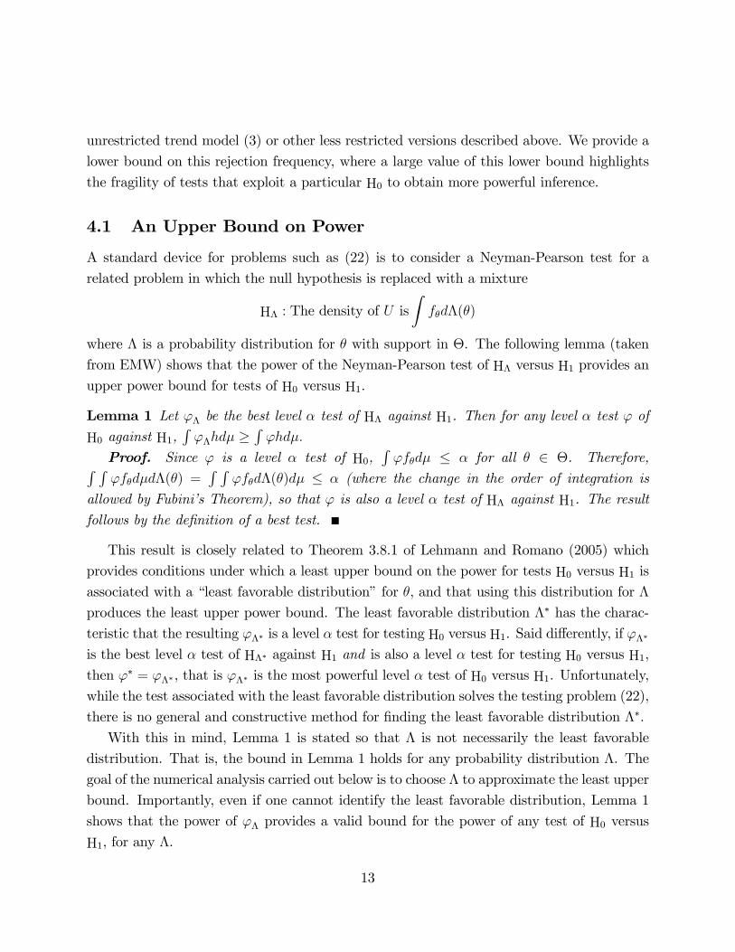
4.1 An Upper Bound on Power

A standard device for problems such as (22) is to consider a Neyman-Pearson test for a

related problem in which the null hypothesis is replaced with a mixture

H� : The density of U isZf�d�(�)

where � is a probability distribution for � with support in �. The following lemma (taken

from EMW) shows that the power of the Neyman-Pearson test of H� versus H1 provides an

upper power bound for tests of H0 versus H1.

Lemma 1 Let '� be the best level � test of H� against H1. Then for any level � test ' of

H0 against H1,R'�hd� �

R'hd�:

Proof. Since ' is a level � test of H0,R'f�d� � � for all � 2 �. Therefore,R R

'f�d�d�(�) =R R

'f�d�(�)d� � � (where the change in the order of integration is

allowed by Fubini�s Theorem), so that ' is also a level � test of H� against H1. The result

follows by the de�nition of a best test.

This result is closely related to Theorem 3.8.1 of Lehmann and Romano (2005) which

provides conditions under which a least upper bound on the power for tests H0 versus H1 is

associated with a �least favorable distribution�for �, and that using this distribution for �

produces the least upper power bound. The least favorable distribution �� has the charac-

teristic that the resulting '�� is a level � test for testing H0 versus H1. Said di¤erently, if '��is the best level � test of H�� against H1 and is also a level � test for testing H0 versus H1,

then '� = '��, that is '�� is the most powerful level � test of H0 versus H1. Unfortunately,

while the test associated with the least favorable distribution solves the testing problem (22),

there is no general and constructive method for �nding the least favorable distribution ��.

With this in mind, Lemma 1 is stated so that � is not necessarily the least favorable

distribution. That is, the bound in Lemma 1 holds for any probability distribution �. The

goal of the numerical analysis carried out below is to choose � to approximate the least upper

bound. Importantly, even if one cannot identify the least favorable distribution, Lemma 1

shows that the power of '� provides a valid bound for the power of any test of H0 versus

H1, for any �.

13

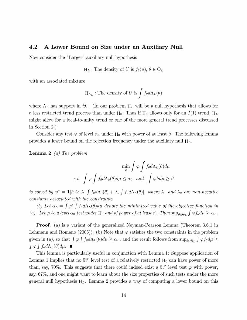
4.2 A Lower Bound on Size under an Auxiliary Null

Now consider the "Larger" auxiliary null hypothesis

HL : The density of U is f�(u), � 2 �L

with an associated mixture

H�L : The density of U isZf�d�L(�)

where �L has support in �L. (In our problem HL will be a null hypothesis that allows for

a less restricted trend process than under H0. Thus if H0 allows only for an I(1) trend, HLmight allow for a local-to-unity trend or one of the more general trend processes discussed

in Section 2.)

Consider any test ' of level �0 under H0 with power of at least �. The following lemma

provides a lower bound on the rejection frequency under the auxiliary null HL.

Lemma 2 (a) The problem

min'

Z'

Zf�d�L(�)d�

s.t.Z'

Zf�d�0(�)d� � �0 and

Z'hd� � �

is solved by '� = 1[h � �1Rf�d�0(�) + �2

Rf�d�L(�)], where �1 and �2 are non-negative

constants associated with the constraints.

(b) Let �L =R'�Rf�d�L(�)d� denote the minimized value of the objective function in

(a). Let ' be a level �0 test under H0 and of power of at least �. Then sup�2�LR'f�d� � �L.

Proof. (a) is a variant of the generalized Neyman-Pearson Lemma (Theorem 3.6.1 in

Lehmann and Romano (2005)). (b) Note that ' satis�es the two constraints in the problem

given in (a), so thatR'Rf�d�L(�)d� � �L, and the result follows from sup�2�L

R'f�d� �R

'Rf�d�L(�)d�.

This lemma is particularly useful in conjunction with Lemma 1: Suppose application of

Lemma 1 implies that no 5% level test of a relatively restricted H0 can have power of more

than, say, 70%. This suggests that there could indeed exist a 5% level test ' with power,

say, 67%, and one might want to learn about the size properties of such tests under the more

general null hypothesis HL. Lemma 2 provides a way of computing a lower bound on this

14

size that is valid for any test with power of at least 67%. So if this size distortion is large,

then without having to determine the class of 5% level tests of H0 with power of at least

67%, one can already conclude that all such tests will be fragile. In the numerical section

below, we discuss how to determine suitable �0 and �L to obtain a large lower bound �L(�1 and �2 are determined through the two constraints on '�).

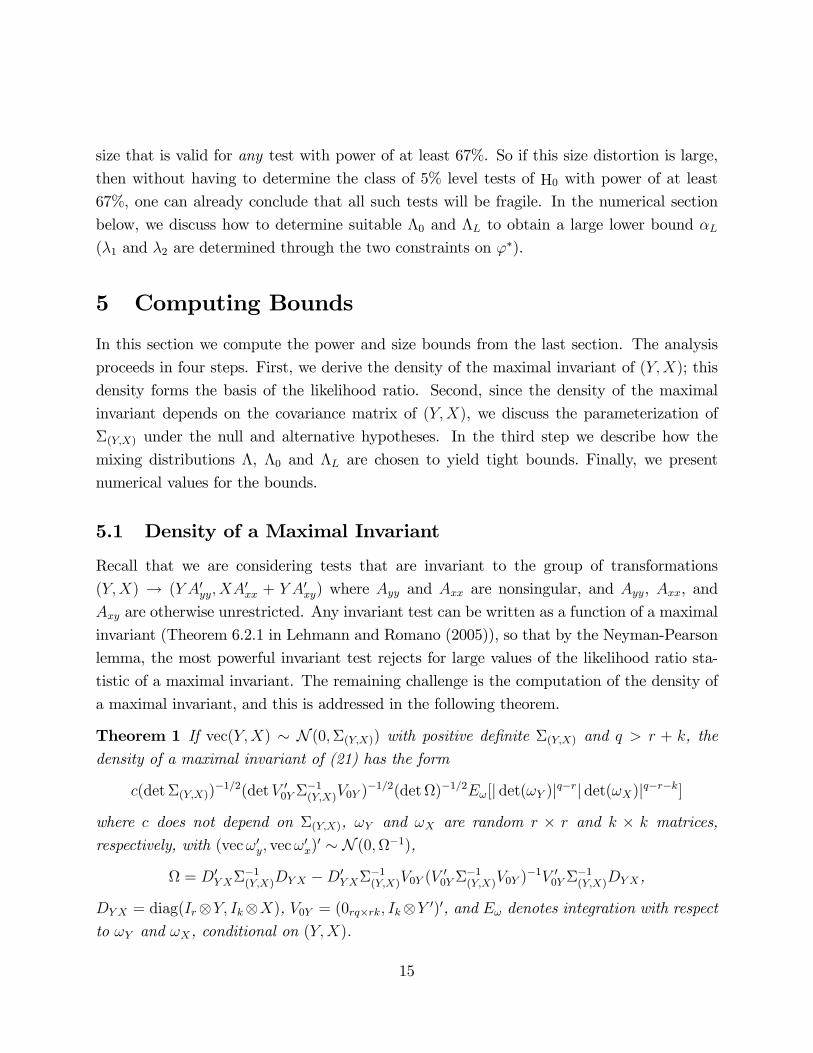
5 Computing Bounds

In this section we compute the power and size bounds from the last section. The analysis

proceeds in four steps. First, we derive the density of the maximal invariant of (Y;X); this

density forms the basis of the likelihood ratio. Second, since the density of the maximal

invariant depends on the covariance matrix of (Y;X), we discuss the parameterization of

�(Y;X) under the null and alternative hypotheses. In the third step we describe how the

mixing distributions �, �0 and �L are chosen to yield tight bounds. Finally, we present

numerical values for the bounds.

5.1 Density of a Maximal Invariant

Recall that we are considering tests that are invariant to the group of transformations

(Y;X) ! (Y A0yy; XA0xx + Y A

0xy) where Ayy and Axx are nonsingular, and Ayy, Axx, and

Axy are otherwise unrestricted. Any invariant test can be written as a function of a maximal

invariant (Theorem 6.2.1 in Lehmann and Romano (2005)), so that by the Neyman-Pearson

lemma, the most powerful invariant test rejects for large values of the likelihood ratio sta-

tistic of a maximal invariant. The remaining challenge is the computation of the density of

a maximal invariant, and this is addressed in the following theorem.

Theorem 1 If vec(Y;X) � N (0;�(Y;X)) with positive de�nite �(Y;X) and q > r + k, the

density of a maximal invariant of (21) has the form

c(det�(Y;X))�1=2(detV 00Y�

�1(Y;X)V0Y )

�1=2(det)�1=2E![j det(!Y )jq�rj det(!X)jq�r�k]

where c does not depend on �(Y;X), !Y and !X are random r � r and k � k matrices,respectively, with (vec!0y; vec!

0x)0 � N (0;�1),

= D0Y X�

�1(Y;X)DY X �D0

Y X��1(Y;X)V0Y (V

00Y�

�1(Y;X)V0Y )

�1V 00Y��1(Y;X)DY X ,

DY X = diag(IrY; IkX), V0Y = (0rq�rk; IkY 0)0, and E! denotes integration with respectto !Y and !X , conditional on (Y;X).

15

Theorem 1 shows that the density of a maximal invariant can be expressed in terms of

absolute moments of determinants of jointly normally distributed random matrices, whose

covariance matrix depends on (Y;X). We do not know of a useful and general closed-form

solution for this expectation; for r = k = 1, however, Nabeya�s (1951) results for the absolute

moments of a bivariate normal yields an expression in terms of elementary functions, which

we omit for brevity. When r + k > 2, the moments can be computed via Monte Carlo

integration. However, computing accurate approximations is di¢ cult when r and k are

large, and the numerical analysis reported below is therefore limited to small values of r and

k.

5.2 Parameterization of �(Y;X)

Since the density of the maximal invariant of Theorem 1 depends on �(Y;X), the derivation

of e¢ cient invariant tests requires speci�cation of �(Y;X) under the alternative and null

hypothesis. We discuss each of these in turn.

5.2.1 Speci�cation of �(Y;X) under the Alternative Hypothesis

As discussed above, we focus on the alternative where the stochastic trends follow an I(1)

process, so that H(s; t) satis�es (6) and (10). There remains the issue of the value of B

(the coe¢ cients that show how the trends a¤ect Y ) and R (the correlation of the Wiener

processes describing the I(0) variables, zt, and the common trends, vt). For these parameters,

we consider point-valued alternatives with B = B1 and R = R1; the power bounds derived

below then serve as bounds on the asymptotic power envelope over these values of B and R.

Invariance reduces the e¤ective dimension of B and R somewhat, and this will be discussed

in the context of the numerical results presented below.

5.2.2 Parameterization of �(Y;X) under the Null Hypothesis

From (20), under the null hypothesis with B = 0, the covariance matrix �(Y;X) satis�es

�(Y;X) =

"Irq �ZV

�V Z �V V

#:

The model�s speci�cation of the stochastic trend under the null determines the rq�kq matrix�ZV and the kq�kq matrix �V V by the formulae given in (17). Since these matrices containa �nite number of elements, it is clear that even for nonparametric speci�cations of H(s; t);

16

the e¤ective parameter space for low-frequency tests based on (Y;X) is �nite dimensional.

We collect these nuisance parameters in a vector � 2 �.Section 2 discussed several trend processes, beginning with the general process given in

(3) with an unrestricted version of H(s; t), and then �ve restricted models: (i) the �G�model

in (6), (ii) the �Diagonal�model (8), (iii) the �Stationary�model (9), (iv) the local-to-unity

model (11), and (v) the I(1) model (10). The appendix discusses convenient parameteriza-

tions for �(Y;X) for these �ve restricted models, and the following lemma provides the basis

for parameterizing �(Y;X) when H(s; t) is unrestricted.

Lemma 3 (a) For any (r+k)q� (r+k)q positive de�nite matrix �� with upper left rq� rqblock equal to Irq; there exists an unrestricted trend model with H(s; t) = 0 for t < 0 such

that �� = E[vec(Z; V )(vec(Z; V ))0].

(b) If r � k, this H(s; t) can be chosen of the form H(s; t) = G(s; t)Sv, where (S 0z; S0v)

has full rank.

The lemma shows that when H(s; t) is unrestricted (or r � k and H(s; t) = G(s; t)Sv

with G unrestricted) the only restriction that the null hypothesis imposes on �(Y;X) is that

�Y Y = Irq.7 In other words, since �ZV and �V V have rkq2+ kq(kq+1)=2 distinct elements,

an appropriately chosen � of that dimension determines �(Y;X) under the null hypothesis in

the unrestricted model, and in the model where H(s; t) = G(s; t)Sv for r � k.

5.3 Approximating the Least Upper Power and Greatest LowerSize Bound

We discuss two methods to approximate the power bound associated with the least favorable

distribution from Section 4, and use the second method also to determine a large lower size

bound. First, we discuss a generic algorithm developed in Elliott, Mueller andWatson (2012)

that simultaneously determines a low upper bound on power, and a level � test whose power

is close to that bound. The computational complexity is such, however, that it can only be

applied when � is low-dimensional; as such, it is useful for our problem only in the I(1) and

local-to-unity stochastic trend model for r = k = 1. Second, when the dimension of � is

7Without the invariance restriction (21), this observation would lead to an analytic least favorable distri-

bution result: Factor the density of (Y;X) under the alternative into the product of the density of Y , and

the density of X given Y . By choosing �V Z and �V V under the null hypothesis appropriately, the latter

term cancels, and the Neyman-Pearson test is a function of Y only. In section 6 below we consider the

e¢ cient Y -only invariant test and compare its power to the approximate (Y;X) power bound.

17

large we choose � (and �0 and �L for Lemma 2) so the null and alternative distributions

are close in a numerically convenient metric. Two numerical results suggest that this second

method produces a reasonably accurate estimate of the least upper power bound: the method

produces power bounds only marginally higher than the �rst method (when the �rst method

is feasible), and when r = 1 we �nd that the method produces a power bound that can be

achieved by a feasible test that we present in the next section.

We discuss the two methods in turn.

5.3.1 Low Dimensional Nuisance Parameter

Suppose that LR� = h(U)=Rf�(U)d�(�) is a continuous random variable for any �, so that

by the Neyman-Pearson Lemma, '� is of the form '� = 1[LR� > cv�], where the critical

value cv� is chosen to satisfy the size constraintR R

'�f�d�d�(�) = �. Then by Lemma

1, the power of '�, �� =R'�hd�, is an upper bound on the power of any test that is

level � under H0. If � is not the least favorable distribution, then '� is not of size � under

H0, i.e. sup�2�R'�f�d� > �. Now consider a version of '� with a size-corrected critical

value cvc� > cv�, that is 'c� = 1[LR� > cv

c�] with cv

c� chosen to satisfy the size constraint

sup�2�R'c�f�d� = �. Because the size adjusted test 'c� is of level � under H0, the least

upper power bound must be between �c� and ��. Thus, if �c� is close to ��, then �

c� serves

as a good approximation to the least upper bound.

The challenge is to �nd an appropriate �: This is di¢ cult because, in general, no closed

form solutions are available for the size and power of tests, so that these must be approx-

imated by Monte Carlo integration. Brute force searches for an appropriate � are not

computationally feasible. Elliott, Müller, and Watson (2012) develop an algorithm that

works well (in the sense that it produces a test with power within ", where " is a small

pre-speci�ed value) in several problems when the dimension of � is small, and we implement

their algorithm here.

5.3.2 High Dimensional Nuisance Parameter

The dimension of � can be very large in our problem: even when r = k = 1, the model with

unrestricted stochastic trend leads to � of dimension q2 + q(q + 1)=2 so that � contains 222

elements when q = 12. Approximating the least upper power bound directly then becomes

numerically intractable. This motivates a computationally practical method for computing

a low (as oppose to least) upper power bound.

18

The method restricts � so that it is degenerate with all mass on a single point, say ��,

which is chosen so that the null distribution of the maximal invariant of Theorem 1 is close to

its distribution under the alternative. Intuitively, this should make it di¢ cult to distinguish

the null from the alternative hypothesis, and thus lead to a low power bound. Also, this

choice of �� ensures that draws from the null model look empirically reasonable, as they are

nontrivial to distinguish from draws of the alternative with an I(1) stochastic trend.

Since the density of the maximal invariant is quite involved, �� is usefully approximated

by a choice that makes the multivariate normal distribution of vec(Y;X) under the null close

to its distribution under the alternative, as measured by a convenient metric. We choose

�� to minimize the Kullback-Leibler divergence (KLIC) between the null and alternative

distributions. Since the bounds from Lemmas 1 and 2 are valid for any mixture, numerical

errors in the KLIC minimization do not invalidate the resulting bound. Details are provided

in the appendix.

5.4 Numerical Bounds

Table 1 shows numerical results for power and size bounds for 5% level tests with q = 12.

Results are shown for r = k = 1 (panel A), r = 1 and k � 2 (panel B), and r = 2 and k = 1(Panel C).8 Numerical results for larger values of n = r + k are not reported because of the

large number of calculations required to evaluate the density of Theorem 2 in large models.

Power depends on the values of B and R under the alternative, and results are presented

for various values of these parameters. Because of invariance, when r = 1 (as in panels A and

B), or k = 1 (as in panel C), the distribution of the maximal invariant depends on B and R

only through jjBjj, jjRjj, and, if jjRjj > 0, on tr(R0B)=(jjBjj � jjRjj). Thus, in panel A, wherer = k = 1, results are shown for two values of jBj, three values of jRj and for R �B < 0 andR � B > 0, while panels B and C show results for three values of ! = tr(R0B)=(jjBjj � jjRjj)when jjRjj > 0. All of the results in Table 1 use the KLIC minimized values of � as describedin the last subsection. Table 2 compares this KLIC-based bounds to to the numerical least

upper power bounds when the parameter space is su¢ ciently small to allow calculation of

the numerical least upper bounds.

To understand the formatting of Table 1, look at panel A. The panel contains italicized

and non-italicized numerical entries. The non-italicized numbers are power bounds, and the

8The results shown in panel B were computed using the KLIC minimized value of � for the model with

r = 1 and k = 2. The appendix shows the resulting bounds are valid for k � 2.

19

italicized numbers are size bounds. The �rst column in the table shows the trend speci-

�cation allowed under H0. The �rst entry, labelled �unr�corresponds to the unrestricted

trend speci�cation in (3) and the other entries correspond to the restricted trend processes

discussed in Section 2. Because r = k = 1, there are no restrictions imposed by the as-

sumption that H(s; t) = G(s; t)Sv or that G is diagonal, so these models are not listed in

panel A. Stationarity (G(s; t) = G(s � t)) is a restriction, and this is the second entry inthe �rst column. The �nal two entries correspond to the local-to-unity (�LTU�) and I(1)

restrictions. The numerical entries shown in the rows corresponding to these trend models

are the power bounds. For example, the non-italicized entries in the �rst numerical column

show power bounds for jRj = 0 and jBj = 7, which are 0:36 for the unrestricted null, 0:41when the trend is restricted to be stationary, 0:50 when the trend is restricted to follow a

local-to-unity process, and 0:50 when the trend is further restricted to follow an I(1) process.

The second column of panel A shows the auxiliary null hypotheses HL, corresponding

to the null hypothesis H0, shown in the �rst column. The entries under HL represent less

restrictive models than H0. For example, when H0 restricts the null to be stationary, an

unrestricted trend process (�unr�) is shown for HL, while when H0 restricts the trend to be

I(1), the less restrictive local-to-unity, stationary, and unrestricted nulls are listed under HL.

The numerical entries for these rows (shown in italics in the table) are the lower size bounds

for HL for 5% level tests under H0 and with power that is 3 percentage points less than

the corresponding power bound shown in the table. For example, from the �rst numerical

column of panel A, the power bound for the I(1) version of H0 is 0:50. For any test with

size no larger than 5% under this null and with power of at least 0:47 (= 0:50 � 0:03), thesize under a null that allows an unrestricted trend (�unr�under HL) is at least 12%, the

size under a null that restricts the trend to be stationary is at least 8%, and the size under

a null that restricts the trend to follow a local-to-unity process is at least 4%.

Looking at the entries in Panel A, two results stand out. First, and not surprisingly,

restricting tests so that they control size for the unrestricted trend process leads to a non-

negligible reduction in power. For example, when jBj = 7, and R = 0, the power bound is0:36, for tests that control size for unrestricted trends, the bound increases to 0:41 for tests

that control size for stationary trends, and increases to 0:50 for tests that control size for

local-to-unity or I(1) trend processes. Second, whenever there is a substantial increase in

power associated with restricting the trend process, there are large size distortions under

the null hypothesis without this restriction. For example, Elliott�s (1998) observation that

e¢ cient tests under the I(1) trend have large size distortions under a local-to-unity process

20

is evident in the table. From the table, when jBj = 7, jRj = 0:9, and R � B > 0, the powerbound for the null with an I(1) trend is 0:95, but any test that controls size for this null and

has power of at least 0:92 will have size that is greater than 0:50 when the trend is allowed to

follow a local-to-unity process. However, addressing Elliott�s (1998) concern by controlling

for size in the local-to-unity model, as in the analysis of Stock and Watson (1996) or Jansson

and Moreira (2006) does not eliminate the fragility of the test. For example, with the same

values of B and R, the power bound for the null that allows for a local-to-unity trend is

0:67, but any test that controls size for this null and has a size of at least 0:64 will have a

size greater than 0:32 when the trend is unrestricted.

Panels B (r = 1 and k = 2) and C (r = 2 and k = 1) show qualitatively similar results.

Indeed these panels show even more fragility of tests that do not allow for general trends.

For example, the lower size bound for the unrestricted trend null exceeds 0:50 in several

cases for tests that restrict trends to be I(1), local-to-unity, or stationary.

When r = k = 1, it is feasible to approximate the least upper power bound for the I(1)

and local-to-unity trend restrictions using the method developed in EMW. By construction,

the approximate least upper bounds (LUB) in Table 2 are no more than 2.5 percentage

points above the actual least upper bound, apart from Monte Carlo error. The di¤erences

with the KLIC minimized power bounds are small, suggesting that the bounds in Table 1

are reasonably tight.

6 E¢ cient Y -Only Tests

The primary obstacle for constructing e¢ cient tests of the null hypothesis that B = 0 is the

large number of nuisance parameters associated with the stochastic trend (the parameters

that determine H(s; t)). These parameters govern the values of �ZV and �V V , which in turn

determine �Y X and �XX . Any valid test must control size over all values of these nuisance

parameters. Wright (2000) notes that this obstacle can be avoided by ignoring the xt data

and basing inference only on yt, since under the null hypothesis, yt = zt. This section takes

up Wright�s suggestion and discusses e¢ cient low-frequency �Y -only�tests.9

9Wright (2000) implements this idea using a �stationarity�test of the I(0) null proposed by Saikkonen and

Luukonen (1993), using a robust covariance matrix as in Kwiatkowski, Phillips, Schmidt, and Shin (1992) for

the test proposed in Nyblom (1989). This test relies on a consistent estimator of the spectral density matrix

of zt at frequency zero. But consistent estimation requires a lot of pertinent low frequency information,

and lack thereof leads to well-known size control problems (see for example, Kwiatkowski, Phillips, Schmidt,

and Shin (1992), Caner and Kilian (2001), and Müller (2005)). These problems are avoided by using the

21

We have two related goals. The �rst is to study the power properties of these tests

relative to the power bounds computed in the last section. As it turns out, when r = 1 (so

there is only a single cointegrating vector), this Y -only test essentially achieves the power

bound, so the test e¢ ciently uses all of the information in Y and X. Given the e¢ ciency

property of the Y -only test, the second goal is to develop simple formulae for implementing

the test. We discuss these in reverse order, �rst deriving a convenient formulae for the test

statistic and then studying the power of the resulting test.

6.1 E¢ cient Tests against General Alternatives

The distribution of vecY � N (0;�Y Y ) follows from the derivations in Section 3: Under the

null hypothesis, �Y Y = Irq, and under the alternative, �Y Y depends on the local alternative

B, the properties of the stochastic trend and its relationship with the error correction term

Z. For a particular choice of alternative, the testing problem thus becomes H0 : �Y Y = Irqagainst H1 : �Y Y = �Y Y 1, and the invariance requirement (21) becomes

Y ! Y A0yy for arbitrary nonsingular r � r matrices Ayy: (23)

The density of the maximal invariant is given in the following theorem.

Theorem 2 (a) If vecY � N (0;�Y Y ) with positive de�nite �Y Y and q > r, the density ofa maximal invariant to (23) has the form

c1(det�Y Y )�1=2(detY )

�1=2E!Y [j det(!Y )jq�r]

where c1 does not depend on �Y Y , !Y is an r � r random matrix with vec!Y � N (0;�1Y ),Y = (Ir Y )0��1Y Y (Ir Y ), and E!Y denotes integration with respect to the distribution of!Y (conditional on Y ).

(b) If in addition, �Y Y = ~VY Y ~�Y Y where ~VY Y is r � r and ~�Y Y is q � q, then thedensity simpli�es to

c2(det ~�Y Y )�r=2 det(Y 0 ~��1Y Y Y )

�q=2

where c2 does not depend on �Y Y :

As in Theorem 1, part (a) of this theorem provides a formula for the density of a maximal

invariant in terms of absolute moments of the determinant of a multivariate normal matrix

low-frequency components of yt only; see Müller and Watson (2008) for further discussion.

22

with a covariance matrix that depends on the data. Part (b) provides an explicit and simple

formula when the covariance matrix is of a speci�c Kronecker form. This form arises under

the null hypothesis with �Y Y = Irq, and under alternatives where each of the r putative

error correction terms in yt have the same low-frequency covariance matrix. For a simple

alternative hypothesis with �Y Y 1 = ~VY Y 1 ~�Y Y 1, the best test then rejects for large valuesof det(Y 0Y )= det(Y 0 ~��1Y Y 1Y ). The form of weighted average power maximizing tests over a

set of alternative covariance matrices �Y Y 1 are also easily deduced from Theorem 2.

6.2 E¢ cient Tests against I(1) Alternatives

As discussed above, the numerical results in this paper focus on the benchmark alterna-

tive where the stochastic trend follows an I(1) process. Under this alternative, yt follows

a multivariate �local level model�(cf. Harvey (1989)), which is the alternative underlying

well-known �stationarity� tests such as Nyblom and Mäkeläinen (1983), Nyblom (1989),

Kwiatkowski, Phillips, Schmidt, and Shin (1992), Nyblom and Harvey (2000), Jansson

(2004), and others. Thus, suppose that the stochastic trend satis�es (6) and (10), so that

T�1=2bsT cXt=1

yt ) Wz(s) +B

Z s

0

Wv(t)dt: (24)

The optimal test therefore depends on the value of B and the correlation matrix R =

SzS0v = E[Wz(1)Wv(1)

0] under the alternative. The invariance constraint (23), as well as the

properties of �Y Y arising under (24) lead to certain cancellations and simpli�cations, that

we discuss in detail in the appendix. The end-result is the following Corollary to Theorem

2.

Corollary 1 LetLFST(b) = det(Y 0Y )= det(Y 0(Iq + b2D)�1Y ) (25)

for some scalar b > 0, where D = diag(��2; (2�)�2; � � � ; (q�)�2).(a) When r = 1, the test that rejects for large values of LFST(b) is uniformly most

powerful against all alternatives (24) with jjBjj = b and any value of R.(b) When 1 < r � k, the test that rejects for large values of LFST(b) is uniformly most

powerful against all alternatives (24) with B and R such that the r eigenvalues of BB0 are

equal to b2, and there exists an orthogonal k� k matrix Qk for which BQkR0 is a symmetricr � r matrix.

23

The statistic (25) was developed as a "low-frequency stationarity test" and denoted

"LFST" in Müller and Watson (2008) and we continue to use that label here. The corollary

suggests that the LFST is a powerful Y -only test for inference about the cointegrating vector

in a variety of cases. When r > k, the point optimal test statistic under similar conditions

as described in part (b) of the Corollary is given by �(b) derived in the appendix. In contrast

to LFST(b), the statistic �(b) does not have a simple closed-form expression, as it involves

the form of the density of the maximal invariant derived in part (a) of Theorem 2.

As a practical matter, it is much more convenient to continue to rely on LFST(b) with

Y = YT even if r > k, although at the cost of somewhat reduced power, as discussed in

the next subsection. Table 3 presents 10%, 5%, and 1% critical values for the point-optimal

LFST(10=pr) for various values of r and q, where the alternative b = 10=

pr is chosen

so that the 5% level test has approximately 50% power (cf. King (1988)). Since the low-

frequency transformation of the putative error correction terms YT are linear functions of

the hypothesized cointegrating vector(s), the boundaries of the con�dence set obtained by

inverting the point-optimal LFST (that is, the values of �0 that do not lead to a rejection)

simply solve a quadratic equation. The �nding of an empty con�dence set may be interpreted

as evidence against the notion that the system satis�es r � 1 cointegrating relationships.

6.3 Power of E¢ cient Y -only Tests

Table 4 shows the power of the point-optimal LFST and the corresponding power envelope

of the Y -only test for r = 1 in panel A, and r = 2 and k = 1 in panel B. In panel A,

the power envelope is given by the LFST(b) evaluated at the value of b = B under the

alternative, while the point-optimal LFST is evaluated at b = 10. The power of the point-

optimal test is very close to the Y -only power envelope. A more interesting comparison

involves the power of the point-optimal LFST with the (Y;X)-power bound computed in

the last section. Because the Y -only tests control size for any trend process, the relevant

comparison is the unrestricted H(s; t) bound shown in panels A and B of Table 1. The power

of the point-optimal LFST di¤ers from the Table 1 power bound by no more than 0:01 when

jBj = 7 and by no more than 0:03 when jBj = 14. Thus, for all practical purposes, the

point-optimal LFST corresponds to an e¢ cient test in models with a single cointegrating

vector (r = 1).

The results in panel B of Table 4 are somewhat di¤erent. Here, because r > k = 1, the

Y -only power envelope is computed using the �(jjBjj) statistic derived in the appendix, andnot by the LFST. The numerical results show that the relative power of the LFST depends

24

on both B and R, and the loss can be large when B and R are large and orthogonal (! = 0).

Comparing the results in panel B of Table 4 to the corresponding results in panel C of Table

1 shows that in this case there are potentially additional power gains associated with using

data on both Y and X. For example, when jjBjj = 20, jjRjj = 0:9, and ! = 0, the Y -onlypower envelope is 0:86, while the (Y;X) power bound is 0:94.

7 Interest Rates and the Term Spread

Figure 1 plots monthly values of the 1 year and 10 year U.S. Treasury bond rates (R1Year and

R10Year) from 1953:4-2011:12. Evidently, both series are persistent, but over long periods they

closely move together, suggesting a common source of long-run variability. Figure 2 plots

the monthly values of the term spread, the di¤erence between R10Year and R1Year. This series

appears to be less persistent than the levels of the interest rates in Figure 1. Taken together,

the �gures suggest R10Year and R1Year are cointegrated with a cointegrating coe¢ cient that

is close to unity.

The �rst two rows of Table 5 show statistics that summarize the persistence in the levels

of R1Year and R10Year. Elliott, Rothenberg and Stock�s (1996) DFGLS test does not reject the

null hypothesis of a unit root in the series, and the 95% con�dence interval for the largest

AR root constructed by inverting the Dickey-Fuller statistic (Stock (1991)), yields a range of

values between 0:98 and 1:00 for both interest rates. The usual Nyblom/KPSS (cf. Nyblom

(1989) and Kwiatkowski, Phillips, Schmidt, and Shin (1992)) statistic rejects the I(0) null

with a p-value of less than 1%. The estimates of the long-memory fractional integration

parameter d constructed from Geweke and Porter-Hudak (1983) regressions (implemented

as described in Robinson (2003)) suggest values of d that di¤er from d = 0 (from levels

versions of the regression), but also di¤er from d = 1 (from the di¤erences version of the

regression). Finally, the LFST with q chosen to capture below business cycle frequency

(periods greater than 8 years) rejects the I(0) null for the levels of the two series. Taken

together these results suggest that the levels of the interest rates are highly persistent, but

with a stochastic trend process that might well di¤er from the exact I(1) model.

Figure 2 suggests a value of the cointegrating coe¢ cient that is equal to unity, but

other values are equally plausible. To take one example, consider a simple version of the

expectations theory of the term structure in which R10Yeart = 110

P9i=0R

1Yeart+ijt + et, where

R1Yeart+ijt is the time t expectation of R1Yeart+i and et is an I(0) term premium. Suppose that

R1Yeart follows an AR(1) model with coe¢ cient �. In this case R10Yeart = �(�)R1Yeart + et with

25

�(�) = 1 when � = 1 and �(�) = 1101��101�� for � 6= 1. When � is close to unity, the interest

levels are highly persistent, but R10Yeart � �(�)R1Yeart is not, so that �(�) is the cointegrating

coe¢ cient. Note that �(�) can sharply di¤er from � = 1 even when � is close unity. For

example, �(0:99) = 0:96 and �(0:98) = 0:91.10

Estimating � using using Johansen�s ML estimator in a VECM with 12 lags producesb� = 0:96 with a standard error of 0:06. Thus, this I(1) estimator does not reject the nullthat � = 1. Given the uncertainty about the exact nature of the trend process, it is useful to

ask whether this result is robust to alternative models. This is investigated in the �nal row

of Table 5, which summarizes the persistence properties of the term spread. The DFGLS

test rejects the unit root null, although the 95% con�dence interval for the largest root still

suggests considerable persistence. This persistence is also evident in the GPH regression

estimate of d, and the small p-value of the Nyblom/KPSS statistic. However, the LFST

does not reject the I(0) null and so fails to reject the null hypothesis that � = 1. The

low-frequency behavior of the term spread is thus consistent with the I(0) model, that is

the data does not reject the notion that all persistence and other non-i.i.d. dynamics of the

term spread are associated with variations at business cycle or higher frequencies. Non-trivial

business cycle dynamics are, of course, highly plausible for the term spread, so that the low-

frequency focus of the LFST becomes a potentially attractive notion of cointegration in this

setting. In contrast, the more traditional measures in Table 5 that indicate some degree of

deviation from the I(0) model all depend on a relatively wider range of frequencies.11

Finally, while a value of � = 1 is not rejected using standard I(1) inference or low-

frequency inference that is robust to the I(1) trend speci�cation, there are a range of other

values that are not rejected. The 95% con�dence interval for � constructed using the stan-

dard I(1) estimates ranges from 0:83 to 1:08. The coverage of this con�dence interval is

suspect, though, because of its reliance on the I(1) trend speci�cation. Inverting the LFST

statistic produces a con�dence interval that ranges from 0:85 to 1:31. Thus the robust pro-

cedure yields a similar lower bound for the con�dence interval, but a higher upper bound.

10Valkanov (2003) uses this observation in a local-to-unity framework to estimate the local-to-unity para-

meter by inverting an estimate of the cointegrating coe¢ cient �(�).11For instance, the GPH regressions, which yield estimates of d signi�cantly di¤erent from zero, rely

on a reasonably large number of periodogram ordinates (bT 0:65c = 71), which contain information about

periodicities as low as 10 months.

26

A Appendix

A.1 Proof of Theorem 1

Write Y = (Y 01 ; Y02 ; Y

03)0 and X = (X 0

1; X02; X

03)0, where Y1 and X1 have r rows, and Y2 and X2 have

k rows. Consider the one-to-one mapping h : Rq�n 7! Rq�n with

h(Y;X) = Q =

0B@ QY 1 QX1

QY 2 QX2

QY 3 QX3

1CA =

0B@ Y1 Y �11 X1

Y2(Y1)�1 X2 � Y2Y �11 X1

Y3(Y1)�1 (X3 � Y3Y �11 X1)(X2 � Y2Y �11 X1)

�1

1CA :

A straightforward calculation shows that (vecQ0Y 2; vecQ0Y 3; vecQ

0X3) is a maximal invariant to

(21). The inverse of h is given by

h�1(Q) =

0B@ QY 1 QY 1QX1

QY 2QY 1 QX2 +QY 2QY 1QX1

QY 3QY 1 QX3QX2 +QY 3QY 1QX1

1CA :

Using matrix di¤erentials (cf. Chapter 9 of Magnus and Neudecker (1988)), a calculation shows

that the Jacobian determinant of h�1 is equal to (detQY 1)q�r+k(detQX2)q�k�r. The density of Q

is thus given by

(2�)�qn=2(det�(Y;X))�1=2jdetQY 1jq�r+kjdetQX2jq�k�r exp[�1

2(vech�1(Q))0��1(Y;X)(vech

�1(Q))]

and we are left to integrate out QY 1, QX1 and QX2 to determine the density of the maximal

invariant.

Now consider the change of variables from QY 1, QX1, QX2 to !Y , !X and !Y X

QY 1 = Y1!Y

QX1 = !�1Y Y �11 X1!X � !�1Y !Y X

QX2 = (X2 � Y2Y �11 X1)!X

with Jacobian determinant (detY1)r(det(X2 � Y2Y�11 X1))

k det(�!Y )�k. Noting that with this

change, h�1(Q) = (Y !Y ; X!X�Y !Y X), we �nd that the density of the maximal invariant is equalto Z

(2�)�qn=2(det�(Y;X))�1=2jdetY1jq+kjdet(X2 � Y2Y �11 X1)jq�rjdet!Y jq�rjdet!X jq�k�r

� exp[�12 vec(Y !Y ; X!X � Y !Y X)

0��1(Y;X) vec(Y !Y ; X!X � Y !Y X)]d(vec!0Y ; vec!

0X ; vec!

0Y X)

0:

27

Since vec(Y !Y ; X!X � Y !Y X) = DY X vec(!Y ; !X)� V0Y vec(!Y X), we have

vec(Y !Y ; X!X � Y !Y X)0��1(Y;X) vec(Y !Y ; X!X � Y !Y X)

= vec(!Y ; !X)0D0Y X�

�1(Y;X)DY X vec(!Y ; !X)

� 2 vec(!Y ; !X)D0Y X�

�1(Y;X)V0Y vec(!Y X) + vec(!Y X)

0V 00Y ��1V0Y vec(!Y X):

The result now follows from integrating out !Y X by �completing the square�.

A.2 Proof of Theorem 2

The proof to part (a) mimics the proof to Theorem 1 and is omitted. To prove part (b),

note that because of invariance, we can set ~VY Y = Ir without loss of generality, so that

det�Y Y = (det ~�Y Y )r, Y = (Ir Y 0 ~��1Y Y Y ) and (detY )

�1=2 = det(Y 0 ~��1Y Y Y )�r=2. Since

(vec!Y )0Y (vec!Y ) = tr(!0Y Y

0 ~��1Y Y Y !Y ), the density in part (a) of the Theorem becomes pro-

portional to

(det ~�Y Y )�r=2 det(Y 0 ~��1Y Y Y )

�r=2Zjdet!Y jq�r exp[�1

2 tr(!0Y Y

0 ~��1Y Y Y !Y )]d(vec!Y ).

Let ~!Y = (Y 0 ~��1Y Y Y )

1=2!Y , so that jdet!Y jq�r = det(Y 0 ~��1Y Y Y )�(q�r)=2jdet ~!Y jq�r and vec!Y =(Ir (Y 0 ~��1Y Y Y )�1=2) vec ~!Y , and the Jacobian determinant of the transformation from !Y to ~!Yis det(Ir (Y 0 ~��1Y Y Y )�1=2) = (Y 0 ~�

�1Y Y Y )

�r=2. Thus, the density is proportional to

(det ~�Y Y )�r=2 det(Y 0 ~��1Y Y Y )

�q=2Zjdet ~!Y jq�r exp[�1

2 tr(~!0Y ~!Y )]d(vec ~!Y ),

and the result follows.

A.3 Proof of Lemma 3

We �rst establish a preliminary result.

Lemma 4 For any t > 0 and integer �, the functions l : [0; t] 7! R with l(s) =p2 cos(�ls);

l = 1; � � � ; � are linearly independent.

Proof. Choose any real constants cj , j = 1; � � � ; �, so thatP�j=1 cjj(s) = 0 for all s 2 [0; t].

Then alsoP�j=1 cj

(i)j (0) = 0 for all i > 0, where (i)j (0) is the ith (right) derivative of j at

s = 0. A direct calculation shows (i)j (0) = (�1)i=2p2(�j)i for even i. It is not hard to see that

the � � � matrix with j,ith element (�1)i=2(�j)i is nonsingular, so thatP�j=1 cj

(i)j (0) = 0 for

i = 2; 4; � � � ; 2� can only hold for cj = 0, j = 1; � � � ; �.

28

For the proof Lemma 3 we construct H(s; t) such vecZ =R 10 (Ir (t))SzdW (t) and vecV =R 1

0

R 1t (H(s; t)(s))ds dW (t) have the speci�ed covariance matrix. The proof of the slightly more

di¢ cult part (b), where H(s; t) = G(s; t)Sv, is based on the following observations:

(i) Ignoring the restriction on the form of vecV , it is straightforward to construct an appro-

priate multivariate normal vector vecV from a linear combination of vecZ and �, where

� � N (0; Ikq�kq) independent of Z.

(ii) Suppose that R = S was allowed, where S = (Ir; 0r�(k�r)). Then Sz = SSv, vecZ �R 10 FZ(t)SvdW (t) for FZ(t) = S (t), and one can also easily construct � as in (i) via� =

R 10 F�(t)SvdW (t) by an appropriate choice of F� . Since Ito-Integrals are linear, one

could thus write vecV =R 10 F (t)SvdW (t) with F a linear combination of FZ and F� , using

observation (i).

(iii) For any matrix function F : [0; 1] 7! Rkq�k that is equal to zero on the interval (1� "; 1] for

some " > 0, one can set G(s; t) = (Ik (s)0J(t)�1)F (t), where J(t) =R 1t (s)(s)

0ds and

obtainR 10

R 1t (G(s; t) (s))ds SvdW (t) =

R 10 F (t)SvdW (t), since for any matrix A with k

rows and vector v, A v = (Ik v)A.

The following proof follows this outline, but three complications are addressed: R = S is not

allowed; the matrix function F needs to be zero on the interval (1 � "; 1], which does not happen

automatically in the construction in (ii); one must verify that the processR s0 G(s; t)SvdW (t) admits

a cadlag version.

Set Sz to be the �rst r rows of In. Since l(1� s) = (�1)ll(s) for all l � 1, Lemma 4 impliesthat J(t) =

R 1t (s)(s)

0ds and Iq � J(t) are nonsingular for any t 2 (0; 1). The rq � 1 randomvector vecZ" =

R 1�"0 (Sz (s))dW (s) thus has nonsingular covariance matrix Ir �"q, where

�"q = Iq � J(1� "). Also, since

�� =

Ir Iq �12

�21 �22

!is positive de�nite, so is Irq � �12��122 �21, so that we can choose 0 < " < 1 such that Ir �"q ��12�

�122 �21 is positive de�nite. With that choice of ", also �22 � �21(Ir �"q)�1�12 is positive

de�nite.

For part (a) of the lemma, de�ne the [0; 1] 7! Rkq�n function Fa(t) = Aa(In (t)), whereAa = (Aa1; Aa2) with Aa1 = �21(Ir�"q)�1 and Aa2 = (�22��21(Ir�"q)�1�12)1=2(Ik(�"q)�1=2).

For part (b) of the lemma, choose 0 < � < 1 so that �22 � ��2�21(Ir �"q)�1�12 is positivede�nite. Set Sv = (diag(�Ir; Ik�r); (

p1� �2Ir; 0r�(k�r))0), so that R = SzS

0v = �S. Let ~1(s) be

scaled residuals of a continuous time projection of 1[s � 1� "]q+1(s) on f1[s � 1� "]l(s)gql=1 onthe unit interval, and let ~j(s), j = 2; � � � ; kq be the scaled residuals of continuous time projections

29

of 1[s � 1� "]q+j(s) on f1[s � 1� "]l(s)gql=1 and f1[s � 1� "] ~l(s)gj�1l=1 . By Lemma 4,

~j(s),

j = 1; � � � ; kq, are not identically zero, and we can choose their scale to make them orthonormal.

De�ne ~(s) = (~1(s); � � � ; ~kq(s))0, the k � 1 vector �k = (1; 0; � � � ; 0)0, and Ab = (Ab1; Ab2) withAb1 = ��1�21(Ir�"q)�1 and Ab2 = (�22���2�21(Ir�"q)�1�12)1=2. Now de�ne the [0; 1] 7! Rkq�n

function

Fb(t) = Ab

S (t)�0k ~(t)

!Sv:

For both parts, that is for i 2 fa; bg, set

Hi(s; t) = (Ik (s)0J(t)�1)Fi(t) for t 2 [0; 1� "]

and Hi(s; t) = 0 otherwise. With this choice

vecVi =

Z 1

0

Z 1

t(Hi(s; t)(s))ds dW (t)

=

Z 1�"

0

Z 1

t((Ik (s)(s)0J(t)�1)Fi(t))ds dW (t)

=

Z 1�"

0Fi(t)dW (t):

Thus

E[(vecVi)(vecVi)0] =

Z 1�"

0Fi(t)Fi(t)

0dt

E[(vecVi)(vecZ)0] =

Z 1�"

0Fi(t)(Sz (t))0dt

since vec(Z � Z") =R 11�"(Ir (t))SzdW (t) is independent of vecVi. A direct calculation

now shows thatR 1�"0 Fa(t)Fa(t)

0dt = Aa(In �"q)A0a,R 1�"0 Fa(t)(Sz (t))0dt = Aa(S

0z �"q),R 1�"

0 Fb(t)Fb(t)0dt = Ab diag(Ir �"q; Ikq)A0b and

R 1�"0 Fb(t)(Sz (t))0dt = �Ab(S

0z �"q), so that

from the de�nitions of Ai, E[(vecVi)(vecVi)0] = �22 and E[(vecVi)(vecZ)0] = �21, as required.

It thus remains to show that the processesR s0 Hi(s; t)dW (t), i 2 fa; bg, admit a cadlag version.

Recall that jjAjj is the Frobenius norm of the real matrix A, jjAjj =ptrA0A, which is submul-

tiplicative. If v � N (0;�), then E[jjvjj4] = E[(v0v)2] = 2 tr(�2) + (tr�)2 � 3(tr�)2, so that withR ts Hi(u; �)dW (�) � N (0;

R ts Hi(u; �)Hi(u; �)

0d�), we �nd

E[jjZ t

sHi(u; �)dW (�)jj4] � 3(tr

Z t

sHi(u; �)Hi(u; �)

0d�)2

� 3(

Z t

sjjHi(u; �)jj2d�)2:

30

Thus, for 0 � s < t � 1, we have with (s) = d(s)=ds

E[jjZ t

0Hi(t; �)dW (�)�

Z s

0Hi(s; �)dW (�)jj4]

= E[jjZ s

0(Hi(t; �)�Hi(s; �))dW (�) +

Z t

sHi(t; �)dW (�)jj4]

� 3[

Z s

0jjHi(t; �)�Hi(s; �)jj2d�+

Z t

sjjHi(t; �)jj2d�]2

� 3[k2( sup0���1�"

jjJ(�)�1jj2jjFi(�)jj2)(jj(s)�(t)jj2 + (t� s) sup0���1

jj(�)jj2)]2

� 3k4( sup0���1�"

jjJ(�)�1jj4jjFi(�)jj4)( sup0���1

jj (�)jj2 + sup0���1

jj(�)jj2)2(t� s)2

where the last inequality follows from (t) � (s) = (t � s)R 10 (s + �(t � s))d�, so that by

Kolmogorov�s continuity theorem (p. 14 of Oksendal (2000)), there exist continuous (and thus

cadlag) versions of the stochastic processesR s0 Hi(s; t)dW (t), i 2 fa; bg:

A.4 Parameterization of �(Y;X) under H0 in the restricted trendmodels

G-model with r > k: Because of invariance, it is without loss of generality to assume that the �rst

r�k rows of R are equal to zero, so that the �rst r�k columns of Z are independent of V . The jointdistribution of V and the last k rows of Z are then just as in the model with r = k, so that Lemma

3 implies that in the G-model with r > k, �(Y;X) is of the form �(Y;X) = diag(Ir�k Iq;��k) underthe null hypothesis, where ��k is any positive de�nite k

2q�k2q matrix with upper left kq�kq blockequal to the identity matrix. The nuisance parameter � is thus of dimension k2q2 + kq(kq + 1)=2

Diagonal G-model: Let ZV and � be q�k random matrices with vec(Z;ZV ; �) � N (0;�(Z;ZV ;�)),where

�(Z;ZV ;�) = diag

"Ir R

R0 Ik

#; Ik

! Iq:

A construction as in the proof of Lemma 3 implies that the j�th column of V can be chosen as

an arbitrary linear combination of the j�th column of ZV and the j�th column of �, j = 1; � � � ; k(subject to the constraint that the resulting matrix is positive de�nite). Thus, �(Y;X) may be

parametrized as �(Y;X) = A(Z;ZV ;�)�(Z;ZV ;�)A0(Z;ZV ;�)

, where

A(Z;ZV ;�) =

Irq 0 0

0 diag(AV;1; AV;2; � � � ; AV;k) diag(L�;1; L�;2; � � � ; L�;k)

!;

AV;j are arbitrary q � q matrices and L�;j are arbitrary lower triangular q � q matrices. Including

R, � is thus of dimension rk + kq2 + kq(q + 1)=2.

31

In the stationary diagonal model where G(s; t) = diag(gS1 (s� t); � � � ; gSk (s� t)), we set gSj to bestep functions

gSj (x) =

ngXi=1

�j;i1

�i� 1ng + 1

� x

1 + x<

i

ng + 1

�(26)

for ng = 40 and some scalar parameters �j;i, j = 1; � � � ; k, i = 1; � � � ; ng. The steps occur at thepoints i=(ng + 1 � i); so that more �exibility is allowed for small values of x (half of the points

are associated with values of x less than 1, for example). The values of �ZV and �V V then follow

from (17). In this speci�cation � contains the kng coe¢ cients �j;i and the rk coe¢ cients in the

correlation matrix R. While the speci�cation (26) only captures a subset of all possible covariance

matrices �(Y;X) in the (nonparametric) stationary model, any test that controls size for all functions

H(s; t) of the form H(s; t) = diag(gS1 (s� t); � � � ; gSk (s� t))Sv a fortiori has to control size for the

speci�cation (26). The upper bounds on power of tests that control size for all values of � under

(26) are therefore also upper bounds for tests that control size for the generic stationary stochastic

trend model.

In the local-to-unity model, a straightforward (but tedious) calculation determines the value

of �(Y;X) as function of the k � k matrix C and the r � k correlation matrix R, so that � is of

dimension k2+ rk. Finally, the I(1) model is a special case of the local-to-unity model with C = 0:

A.5 Kullback-Leibler Divergence Problem of Section 5.3.2

Let �1 denote the covariance matrix of vec(Y;X) under a speci�c I(1) alternative as described in

Subsection 5.2.1 (that is, for speci�c values of B = B1 and R = R1), let �0(�) with � 2 � be the

covariance matrix of vec(Y;X) under the null for the relevant restrictions on the stochastic trend,

and de�ne the nq � nq matrix (recall that n = r + k)

A( ) =

" yz Iq 0

xz Iq xv Iq

#

where yz is r�r, xz is k�r, and xv is k�k. This yields A( ) vec(Y;X) � N (0; A( )�0(�)A( )0).Denote the Kullback-Leibler divergence between the nq � 1 distributions N (0;�1) and N (0;�0)as K(�1;�0) = 1

2 ln(det�1=det�0) +12 tr(�

�10 �1) � nq. The value of �� is chosen to numerically

solve

min 2Rr2+k2+kr

K(�1; A( )�0(��)A( )0) = min

�2�; 2Rr2+k2+krK(�1; A( )�0(�)A( )

0), (27)

that is, �� numerically minimizes the Kullback-Leibler divergence (or KLIC) between the null and

alternative densities of (Y;X), allowing for transformations as described by A( ) under the null.

While these transformations do not a¤ect the implied distribution of the maximal invariant, they

do in general lead to a di¤erent ��, which we found to yield a slightly lower upper bound. The

32

minimization problem is over a high dimensional parameter, but the objective function is quickly

computed and well behaved, so that numerical minimization is feasible.

A.6 Validity of r = 1; k = 2 bounds for r = 1; k > 2

Here we show that the power bounds computed using r = 1 and k = 2 also serve as power bounds

for models with r = 1 and all values of k > 2.

To see why, �rst consider the alternative I(1) model as described in subsection 5.2.1, Y =

Z+V B0 and X = V . Let P be a k�k orthonormal matrix whose last k�2 rows are orthogonal toR and B, and whose second row is orthogonal to R. Partition X = (X12; X3k), where X12 contains

the �rst two columns of X and X3k contains the remaining k � 2 columns. By invariance, there isno loss in generality in setting X = ~XP = ( ~X12; ~X3k)P; so that Y = Z + ~XPB0 = Z + ~X12B

012,

where ~X12 and B12 are the �rst two columns of ~X and B, respectively, and the last k � 1 columnsof ~X (and thus ~X3k) are independent of Z. The group of transformations

(Y; ~X12; ~X3k)! (Y Ayy; ~X12 ~Axx + Y Axy; ~X3k) (28)

for nonsingular Ayy and ~Axx is a subset of the transformations (Y; ~X) ! (Y Ayy; ~XAxx + Y Axy),

so the best invariant test to (28) is as least as powerful as the best invariant test to (21). Let~Q12 be a maximal invariant to (Y; ~X12) ! (Y Ayy; ~X12 ~Axx + Y Axy), such that f ~Q12; ~X3kg is amaximal invariant to (28). Since ~X3k is independent of (Y; ~X12), the density of f ~Q12; ~X3kg underthe alternative factors as fa; ~Q12 � fa; ~X3k .

For all null models discussed in subsection 5.2.2, it is possible to choose X = (X12; X3k) = V

in a way such that X3k is independent of X12 with marginal distribution f0;X3k = fa; ~X3k , (i.e. it

corresponds to the I(1) model) and the possibilities for X12 and its relationship with Z are the

same as in the version of the model with k = 2. Thus, with this choice, the term fa; ~X3k cancels

in the likelihood ratio test of the maximal invariant to (28), and the testing problem corresponds

precisely to the model with k = 2:12 An upper bound for the model with r = 1 and k = 2 is

therefore also an upper bound for the model with r = 1 and k > 2.

A.7 Derivation of LFST(b) and �(b) of Section 6.2

A straightforward calculation shows that �Y Y can be written as

�Y Y = (Ir Iq) + (BB0 D) + (BR0 F ) + (RB0 F 0) (29)

12This is not strictly true for the stationary G-model, which excludes I(1) stochastic trends. But the low-frequency transformation of the suitably scaled stationary local-to-unity model converges in mean squaredto the I(1) model as the local-to-unity parameter approaches zero (cf. Section 2.4 of Müller and Watson(2008)), so that the additional discriminatory power from X3k can be made arbitrarily small, and theconclusion continues to hold.

33

where F and D are q � q matrices, D is the diagonal matrix de�ned in Corollary 1, and F = [fij ],

with fij = 0 if i and j are both even or odd, and fij = 4=[�2(i2 � j2)] otherwise. Thus, F = �F 0.(The simple diagonal form of D is due to the particular choice of the weighting functions in (14);

see Section 2.3 in Müller and Watson (2008)). Noting that V Q0k has the same distribution as V ,

Y = Z + V B0 implies that �Y Y is the same for B = B1 and B = B1Qk. Thus, if there exists a

suitable Qk that makes BQkR0 symmetric, the last two terms in (29) cancel. The Corollary now

follows from the Neyman-Pearson Lemma and Theorem 2 part (b).

Furthermore, for r > k, assume that BB0 has k eigenvalues equal to b2, and let

Qr diag(b2Ik; 0Ir�k)Q

0r be the spectral decomposition of BB

0. The invariance Y ! Y A0 implies

that the density of the maximal invariant is the same for B1 = B and for B1 = AB. Thus, with

A = Q0r, Q0rBB

0Qr = diag(b2Ik; 0Ir�k), so that by Theorem 2 part (a) and the Neyman-Pearson

Lemma, the best test rejects for large values of

�(b) = det(Y 0Y )(q+k�r)=2 det(Y 0(Iq + b2D)�1Y )�k=2E!Y [jdet(!Y )jq�r]

where vec!Y � N (0;�1Y ) and Y = diag(Ik Y 0(Iq + b2D)�1Y; Ir�k Y 0Y ):

34

References

Andrews, D. W. K. (1991): �Heteroskedasticity and Autocorrelation Consistent Covari-

ance Matrix Estimation,�Econometrica, 59, 817�858.

Baillie, R. T. (1996): �Long Memory Processes and Frational Integration in Economet-

rics,�Journal of Econometrics, 73, 5�59.

Bobkoski, M. J. (1983): �Hypothesis Testing in Nonstationary Time Series,�unpublished

Ph.D. thesis, Department of Statistics, University of Wisconsin.

Campbell, J. Y., and M. Yogo (2006): �E¢ cient Tests of Stock Return Predictability,�

Journal of Financial Economics, 81, 27�60.

Caner, M., and L. Kilian (2001): �Size Distortions of Tests of the Null Hypothesis of

Stationarity: Evidence and Implications for the PPP Debate,� Journal of International

Money and Finance, 20, 639�657.

Cavanagh, C. L. (1985): �Roots Local To Unity,�Working Paper, Harvard University.

Cavanagh, C. L., G. Elliott, and J. H. Stock (1995): �Inference in Models with

Nearly Integrated Regressors,�Econometric Theory, 11, 1131�1147.

Chan, N. H., and C. Z. Wei (1987): �Asymptotic Inference for Nearly Nonstationary

AR(1) Processes,�The Annals of Statistics, 15, 1050�1063.

Chen, W. W., and C. M. Hurvich (2003a): �Estimating Fractional Cointegration in the

Presence of Polynomial Trends,�Journal of Econometrics, 117, 95�121.

(2003b): �Semiparametric Estimation of Multivariate Fractional Cointegration,�

Journal of the American Statistical Association, 463, 629�642.

(2006): �Semiparametric Estimation of Fractional Cointegration Subspaces,�The

Annals of Statistics, 34, 2939�2979.

den Haan, W. J., and A. T. Levin (1997): �A Practitioner�s Guide to Robust Covariance

Matrix Estimation,�in Handbook of Statistics 15, ed. by G. S. Maddala, and C. R. Rao,

pp. 309�327. Elsevier, Amsterdam.

35

Elliott, G. (1998): �The Robustness of Cointegration Methods When Regressors Almost

Have Unit Roots,�Econometrica, 66, 149�158.

Elliott, G., U. K. Müller, and M. W. Watson (2012): �Nearly Optimal Tests When

a Nuisance Parameter is Present Under the Null Hypothesis,�Working Paper, Princeton

University.

Elliott, G., T. J. Rothenberg, and J. H. Stock (1996): �E¢ cient Tests for an

Autoregressive Unit Root,�Econometrica, 64, 813�836.

Elliott, G., and J. H. Stock (1994): �Inference in Time Series Regression When the

Order of Integration of a Regressor is Unknown,�Econometric Theory, 10, 672�700.

Geweke, J., and S. Porter-Hudak (1983): �The Estimation and Application of Long

Memory Time Series Models,�Journal of Time Series Analysis, 4, 221�238.

Granger, C. W. J. (1993): �What Are We Learning About the Long-Run?,�The Eco-

nomic Journal, 103, 307�317.

Harvey, A. C. (1989): Forecasting, Structural Time Series Models and the Kalman Filter.

Cambridge University Press.

Jansson, M. (2004): �Stationarity Testing with Covariates,�Econometric Theory, 20, 56�

94.

Jansson, M., and M. J. Moreira (2006): �Optimal Inference in Regression Models with

Nearly Integrated Regressors,�Econometrica, 74, 681�714.

Jeganathan, P. (1997): �On Asymptotic Inference in Linear Cointegrated Time Series

Systems,�Econometric Theory, 13, 692�745.

Johansen, S. (1988): �Statistical Analysis of Cointegration Vectors,�Journal of Economic

Dynamics and Control, 12, 231�254.

(1991): �Estimation and Hypothesis Testing of Cointegration Vectors in Gaussian

Vector Autoregressive Models,�Econometrica, 59, 1551�1580.

36

Kiefer, N., and T. J. Vogelsang (2005): �A New Asymptotic Theory for

Heteroskedasticity-Autocorrelation Robust Tests,�Econometric Theory, 21, 1130�1164.

Kiefer, N. M., T. J. Vogelsang, and H. Bunzel (2000): �Simple Robust Testing of

Regression Hypotheses,�Econometrica, 68, 695�714.

King, M. L. (1988): �Towards a Theory of Point Optimal Testing,�Econometric Reviews,

6, 169�218.

Kwiatkowski, D., P. C. B. Phillips, P. Schmidt, and Y. Shin (1992): �Testing

the Null Hypothesis of Stationarity Against the Alternative of a Unit Root,�Journal of

Econometrics, 54, 159�178.

Lehmann, E. L., and J. P. Romano (2005): Testing Statistical Hypotheses. Springer, New

York.

Magnus, J. R., and H. Neudecker (1988): Matrix Di¤erential Calculus. Wiley, New

York.

Müller, U. K. (2005): �Size and Power of Tests of Stationarity in Highly Autocorrelated

Time Series,�Journal of Econometrics, 128, 195�213.

(2007): �A Theory of Robust Long-Run Variance Estimation,�Journal of Econo-

metrics, 141, 1331�1352.

(2011): �E¢ cient Tests under a Weak Convergence Assumption,�Econometrica,

79, 395�435.

Müller, U. K., and M. W. Watson (2008): �Testing Models of Low-Frequency Variabil-

ity,�Econometrica, 76, 979�1016.

Nabeya, S. (1951): �Absolute Moments in 2-Dimensional Normal Distribution,�Annals of

the Institute of Statistical Mathematics, 3, 2�6.

Newey, W. K., and K. West (1987): �A Simple, Positive Semi-De�nite, Heteroskedas-

ticity and Autocorrelation Consistent Covariance Matrix,�Econometrica, 55, 703�708.

37

Nyblom, J. (1989): �Testing for the Constancy of Parameters Over Time,�Journal of the

American Statistical Association, 84, 223�230.

Nyblom, J., and A. Harvey (2000): �Tests of Common Stochastic Trends,�Econometric

Theory, 16, 176�199.

Nyblom, J., and T. Mäkeläinen (1983): �Comparisons of Tests for the Presence of

Random Walk Coe¢ cients in a Simple Linear Model,�Journal of the American Statistical

Association, 78, 856�864.

Oksendal, B. (2000): Stochastic Di¤erential Equations: An Introduction with Applications.

Springer, Berlin, 5 edn.

Park, J. Y. (1992): �Canonical Cointegrating Regressions,�Econometrica, 60, 119�143.

Phillips, P. C. B. (1987): �Towards a Uni�ed Asymptotic Theory for Autoregression,�

Biometrika, 74, 535�547.

Phillips, P. C. B., and B. E. Hansen (1990): �Statistical Inference in Instrumental

Variables Regression with I(1) Processes,�Review of Economic Studies, 57, 99�125.

Robinson, P. M. (2003): �Long-Memory Time Series,�in Time Series with Long Memory,

ed. by P. M. Robinson, pp. 4�32. Oxford University Press, Oxford.

Robinson, P. M., and J. Hualde (2003): �Cointegration in Fractional Systems with

Unknown Integration Orders,�Econometrica, 71, 1727�1766.

Robinson, P. M., and D. Marinucci (2001): �Narrow-Band Analysis of Nonstationary

Processes,�The Annals of Statistics, 29, 947�986.

(2003): �Semiparametric Frequency Domain Analysis of Fractional Cointegration,�

in Time Series with Long Memory, ed. by P. M. Robinson, pp. 334�373. Oxford University

Press, Oxford.

Saikkonen, P. (1991): �Estimation and Testing of Cointegrating Regressions,�Economet-

ric Theory, 7, 1�27.

38

Saikkonen, P., and R. Luukonen (1993): �Point Optimal Tests for Testing the Order of

Di¤erencing in ARIMA Models,�Econometric Theory, 9, 343�362.

Stock, J. H. (1991): �Con�dence Intervals for the Largest Autoregressive Root in U.S.

Macroeconomic Time Series,�Journal of Monetary Economics, 28, 435�459.

Stock, J. H., and M. W. Watson (1993): �A Simple Estimator of Cointegrating Vectors

in Higher Order Integrated Systems,�Econometrica, 61, 783�820.

(1996): �Con�dence Sets in Regressions with Highly Serially Correlated Regressors,�

Working Paper, Harvard University.

Sun, Y., P. C. B. Phillips, and S. Jin (2008): �Optimal Bandwidth Selection in

Heteroskedasticity-Autocorrelation Robust Testing,�Econometrica, 76, 175�794.

Valkanov, R. (2003): �Long-Horizon Regressions: Theoretical Results and Applications,�

Journal of Financial Economics, 68, 201�232.

Velasco, C. (2003): �Gaussian Semiparametric Estimation of Fractional Cointegration,�

Journal of Time Series Analysis, 24, 345�378.

Wright, J. H. (2000): �Con�dence Sets for Cointegrating Coe¢ cients Based on Station-

arity Tests,�Journal of Business and Economic Statistics, 18, 211�222.

39

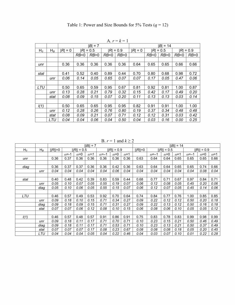
Table 1: Power and Size Bounds for 5% Tests (q = 12)

A. r = k = 1 |B| = 7 |B| = 14

H0 HB |R| = 0 |R| = 0.5 |R| = 0.9 |R| = 0 |R| = 0.5 |R| = 0.9 RB<0 RB>0 RB<0 RB>0 RB<0 RB>0 RB<0 RB>0

unr 0.36 0.36 0.36 0.36 0.36 0.64 0.65 0.65 0.66 0.66

stat 0.41 0.52 0.40 0.89 0.44 0.70 0.80 0.68 0.98 0.72 unr 0.06 0.14 0.05 0.65 0.07 0.07 0.17 0.05 0.47 0.06

LTU 0.50 0.65 0.59 0.95 0.67 0.81 0.92 0.81 1.00 0.87 unr 0.13 0.28 0.21 0.79 0.32 0.15 0.42 0.17 0.49 0.20 stat 0.08 0.09 0.15 0.07 0.20 0.11 0.13 0.13 0.03 0.14

I(1) 0.50 0.65 0.65 0.95 0.95 0.82 0.91 0.91 1.00 1.00 unr 0.12 0.28 0.26 0.76 0.80 0.19 0.37 0.34 0.48 0.48 stat 0.08 0.09 0.21 0.07 0.71 0.12 0.12 0.31 0.03 0.42 LTU 0.04 0.04 0.06 0.04 0.50 0.04 0.03 0.16 0.00 0.25

B. r = 1 and k ≥ 2

||B|| = 7 ||B|| = 14 H0 HB ||R||=0 ||R|| = 0.5 ||R|| = 0.9 ||R||=0 ||R|| = 0.5 ||R|| = 0.9 =-1 =0 =1 =–1 =0 =1 =–1 =0 =1 =–1 =0 =1

unr 0.36 0.37 0.36 0.36 0.36 0.36 0.36 0.63 0.64 0.64 0.65 0.65 0.65 0.66

diag 0.36 0.37 0.37 0.36 0.36 0.42 0.36 0.63 0.64 0.64 0.65 0.65 0.74 0.66 unr 0.04 0.04 0.04 0.04 0.04 0.06 0.04 0.04 0.04 0.04 0.04 0.04 0.08 0.04

stat 0.40 0.48 0.42 0.39 0.83 0.59 0.44 0.68 0.77 0.71 0.67 0.97 0.84 0.71 unr 0.05 0.10 0.07 0.05 0.55 0.19 0.07 0.06 0.12 0.08 0.05 0.45 0.20 0.06 diag 0.05 0.10 0.06 0.05 0.55 0.15 0.07 0.06 0.12 0.07 0.05 0.45 0.14 0.06

LTU 0.46 0.57 0.49 0.53 0.92 0.70 0.64 0.74 0.84 0.77 0.76 1.00 0.85 0.85 unr 0.09 0.18 0.10 0.15 0.71 0.34 0.27 0.09 0.22 0.12 0.12 0.50 0.20 0.18 diag 0.09 0.18 0.09 0.15 0.71 0.31 0.27 0.09 0.22 0.13 0.12 0.50 0.16 0.18 stat 0.07 0.07 0.06 0.12 0.08 0.10 0.15 0.06 0.08 0.06 0.10 0.05 0.05 0.12

I(1) 0.46 0.57 0.48 0.57 0.91 0.86 0.91 0.75 0.83 0.78 0.83 0.99 0.98 0.99 unr 0.09 0.18 0.11 0.17 0.71 0.70 0.71 0.10 0.23 0.15 0.21 0.50 0.46 0.49 diag 0.09 0.18 0.11 0.17 0.71 0.53 0.71 0.10 0.23 0.13 0.21 0.50 0.37 0.49 stat 0.07 0.07 0.07 0.17 0.08 0.23 0.67 0.08 0.08 0.08 0.18 0.05 0.20 0.45 LTU 0.04 0.04 0.04 0.05 0.04 0.22 0.46 0.04 0.03 0.07 0.10 0.01 0.22 0.28

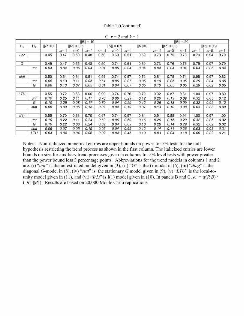
Table 1 (Continued)

C. r = 2 and k = 1 ||B|| = 10 ||B|| = 20

H0 HB ||R||=0 ||R|| = 0.5 ||R|| = 0.9 ||R||=0 ||R|| = 0.5 ||R|| = 0.9 =-1 =0 =1 =–1 =0 =1 =–1 =0 =1 =–1 =0 =1

unr 0.45 0.47 0.50 0.48 0.50 0.69 0.51 0.69 0.73 0.75 0.73 0.79 0.94 0.79

G 0.45 0.47 0.55 0.48 0.50 0.74 0.51 0.69 0.73 0.76 0.73 0.79 0.97 0.79 unr 0.04 0.04 0.06 0.04 0.04 0.06 0.04 0.04 0.04 0.04 0.04 0.04 0.05 0.04

stat 0.50 0.61 0.61 0.51 0.94 0.74 0.57 0.72 0.81 0.78 0.74 0.98 0.97 0.82 unr 0.06 0.13 0.11 0.05 0.61 0.06 0.07 0.05 0.10 0.05 0.05 0.29 0.04 0.05 G 0.06 0.13 0.07 0.05 0.61 0.04 0.07 0.05 0.10 0.05 0.05 0.29 0.02 0.05

LTU 0.55 0.72 0.63 0.66 0.99 0.74 0.76 0.79 0.92 0.87 0.81 1.00 0.97 0.89 unr 0.10 0.25 0.11 0.17 0.70 0.06 0.29 0.12 0.26 0.13 0.09 0.32 0.05 0.12 G 0.10 0.25 0.08 0.17 0.70 0.04 0.29 0.12 0.26 0.13 0.09 0.32 0.02 0.12 stat 0.06 0.09 0.05 0.15 0.07 0.04 0.19 0.07 0.13 0.10 0.08 0.03 0.03 0.09

I(1) 0.55 0.70 0.63 0.70 0.97 0.74 0.97 0.84 0.91 0.88 0.91 1.00 0.97 1.00 unr 0.10 0.22 0.11 0.24 0.69 0.06 0.69 0.16 0.26 0.15 0.29 0.32 0.05 0.32 G 0.10 0.22 0.08 0.24 0.69 0.04 0.69 0.16 0.26 0.14 0.29 0.32 0.02 0.32 stat 0.06 0.07 0.05 0.19 0.05 0.04 0.65 0.12 0.14 0.11 0.26 0.03 0.03 0.31 LTU 0.04 0.04 0.04 0.06 0.02 0.04 0.45 0.10 0.03 0.04 0.18 0.00 0.02 0.21

Notes: Non-italicized numerical entries are upper bounds on power for 5% tests for the null hypothesis restricting the trend process as shown in the first column. The italicized entries are lower bounds on size for auxiliary trend processes given in columns for 5% level tests with power greater than the power bound less 3 percentage points. Abbreviations for the trend models in columns 1 and 2 are: (i) “unr” is the unrestricted model given in (3), (ii) “G” is the G-model in (6), (iii) “diag” is the diagonal G-model in (8), (iv) “stat” is the stationary G model given in (9), (v) “LTU” is the local-to-unity model given in (11), and (vi) “I(1)” is I(1) model given in (10). In panels B and C, = tr(R′B) / (||R||·||B||). Results are based on 20,000 Monte Carlo replications.

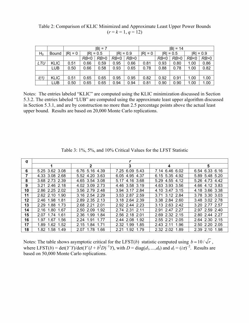
Table 2: Comparison of KLIC Minimized and Approximate Least Upper Power Bounds (r = k = 1, q = 12)

|B| = 7 |B| = 14 H0 Bound |R| = 0 |R| = 0.5 |R| = 0.9 |R| = 0 |R| = 0.5 |R| = 0.9 RB<0 RB>0 RB<0 RB>0 RB<0 RB>0 RB<0 RB>0

LTU KLIC 0.51 0.66 0.59 0.95 0.66 0.81 0.93 0.80 1.00 0.86 LUB 0.50 0.66 0.58 0.93 0.65 0.78 0.88 0.78 1.00 0.82

I(1) KLIC 0.51 0.65 0.65 0.95 0.95 0.82 0.92 0.91 1.00 1.00 LUB 0.50 0.65 0.65 0.94 0.94 0.81 0.90 0.90 1.00 1.00

Notes: The entries labeled “KLIC” are computed using the KLIC minimization discussed in Section 5.3.2. The entries labeled “LUB” are computed using the approximate least upper algorithm discussed in Section 5.3.1, and are by construction no more than 2.5 percentage points above the actual least upper bound. Results are based on 20,000 Monte Carlo replications.

Table 3: 1%, 5%, and 10% Critical Values for the LFST Statistic

q r 1 2 3 4 5

6 5.25 3.62 3.08 6.76 5.16 4.39 7.25 6.09 5.43 7.14 6.46 6.02 6.54 6.33 6.16 7 4.33 3.08 2.68 5.52 4.20 3.63 6.05 4.95 4.37 6.15 5.35 4.92 5.89 5.48 5.20 8 3.68 2.73 2.39 4.65 3.54 3.08 5.17 4.16 3.68 5.29 4.55 4.12 5.26 4.73 4.42 9 3.21 2.46 2.18 4.02 3.09 2.73 4.46 3.58 3.19 4.63 3.93 3.56 4.66 4.12 3.83 10 2.86 2.25 2.02 3.56 2.79 2.48 3.94 3.17 2.84 4.10 3.47 3.15 4.18 3.66 3.38 11 2.62 2.10 1.90 3.16 2.54 2.29 3.53 2.87 2.59 3.71 3.12 2.84 3.78 3.30 3.03 12 2.46 1.98 1.81 2.89 2.35 2.13 3.18 2.64 2.39 3.38 2.84 2.60 3.48 3.02 2.78 13 2.29 1.88 1.73 2.68 2.21 2.01 2.92 2.44 2.23 3.13 2.63 2.42 3.20 2.77 2.57 14 2.16 1.80 1.67 2.50 2.09 1.92 2.74 2.31 2.11 2.91 2.47 2.27 2.97 2.59 2.40 15 2.07 1.74 1.61 2.36 1.99 1.84 2.56 2.18 2.01 2.69 2.32 2.15 2.80 2.44 2.27 16 1.97 1.67 1.56 2.24 1.91 1.77 2.44 2.08 1.92 2.55 2.21 2.05 2.64 2.30 2.15 17 1.89 1.62 1.52 2.15 1.84 1.71 2.32 1.99 1.85 2.43 2.11 1.96 2.50 2.20 2.05 18 1.82 1.58 1.49 2.07 1.78 1.66 2.21 1.92 1.79 2.32 2.02 1.89 2.39 2.10 1.98 Notes: The table shows asymptotic critical for the LFST(b) statistic computed using 10 /b r , where LFST(b) = det(Y´Y)/det(Y´(I + b2D)−1Y), with D = diag(d1,…,dk) and di = (i)–2. Results are based on 50,000 Monte Carlo replications.

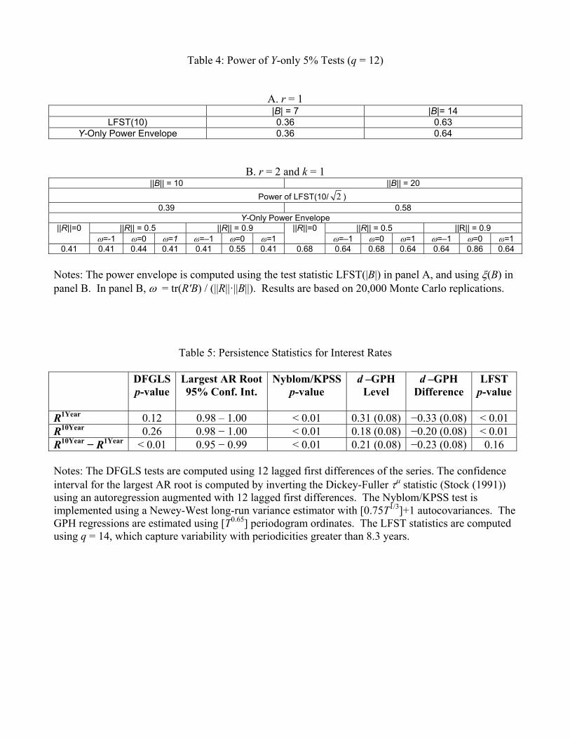
Table 4: Power of Y-only 5% Tests (q = 12)

A. r = 1 |B| = 7 |B|= 14

LFST(10) 0.36 0.63 Y-Only Power Envelope 0.36 0.64

B. r = 2 and k = 1 ||B|| = 10 ||B|| = 20

Power of LFST(10/ 2 ) 0.39 0.58

Y-Only Power Envelope ||R||=0 ||R|| = 0.5 ||R|| = 0.9 ||R||=0 ||R|| = 0.5 ||R|| = 0.9

=-1 =0 =1 =–1 =0 =1 =–1 =0 =1 =–1 =0 =1 0.41 0.41 0.44 0.41 0.41 0.55 0.41 0.68 0.64 0.68 0.64 0.64 0.86 0.64

Notes: The power envelope is computed using the test statistic LFST(|B|) in panel A, and using (B) in panel B. In panel B, = tr(R′B) / (||R||·||B||). Results are based on 20,000 Monte Carlo replications.

Table 5: Persistence Statistics for Interest Rates DFGLS

p-value Largest AR Root 95% Conf. Int.

Nyblom/KPSSp-value

d –GPH Level

d –GPH Difference

LFST p-value

R1Year 0.12 0.98 – 1.00 < 0.01 0.31 (0.08) −0.33 (0.08) < 0.01 R10Year 0.26 0.98 − 1.00 < 0.01 0.18 (0.08) −0.20 (0.08) < 0.01 R10Year − R1Year < 0.01 0.95 − 0.99 < 0.01 0.21 (0.08) −0.23 (0.08) 0.16 Notes: The DFGLS tests are computed using 12 lagged first differences of the series. The confidence interval for the largest AR root is computed by inverting the Dickey-Fuller statistic (Stock (1991)) using an autoregression augmented with 12 lagged first differences. The Nyblom/KPSS test is implemented using a Newey-West long-run variance estimator with [0.75T1/3]+1 autocovariances. The GPH regressions are estimated using [T0.65] periodogram ordinates. The LFST statistics are computed using q = 14, which capture variability with periodicities greater than 8.3 years.

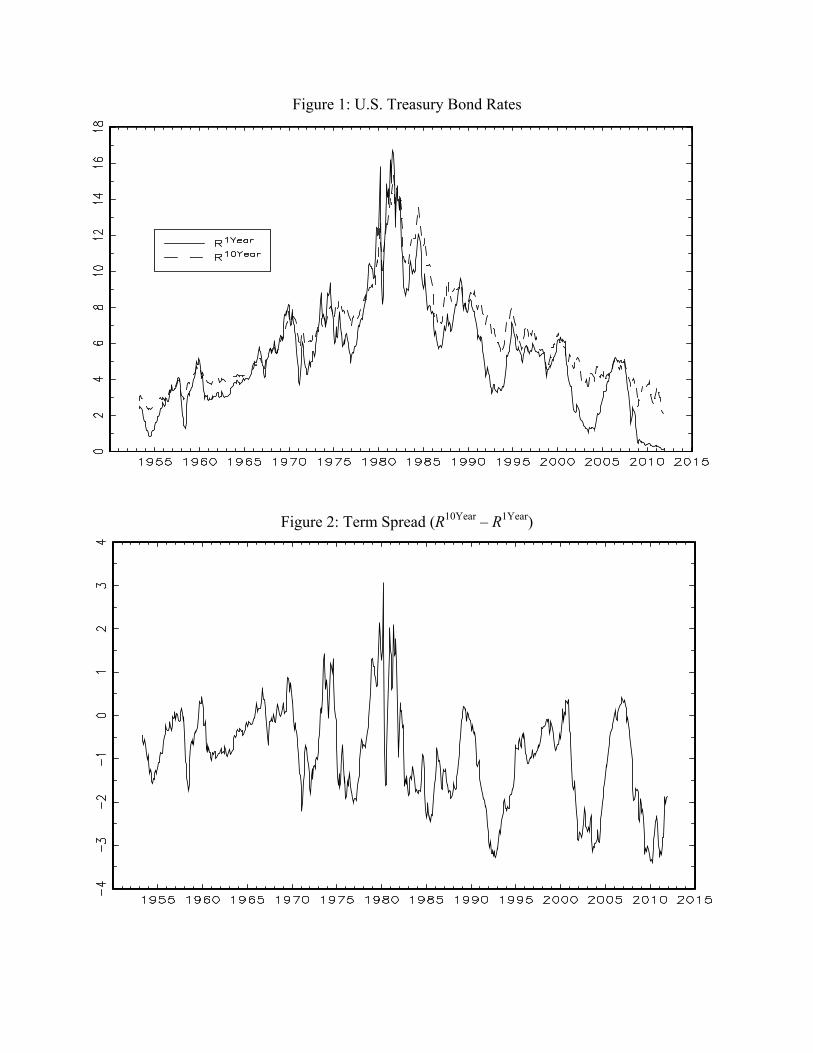
Figure 1: U.S. Treasury Bond Rates

Figure 2: Term Spread (R10Year – R1Year)