Revised: April, 1997

PANEL COINTEGRATION

ASYMPTOTIC AND FINITE SAMPLE PROPERTIES OF POOLED TIME SERIESTESTS WITH AN APPLICATION TO THE PPP HYPOTHESIS

NEW RESULTS

Peter Pedroni

Indiana University

mailing address: Economics, Indiana University Bloomington, IN 47405

(812) 855-7925

email: PPEDRONI@INDIANA.EDU

*Ackowledgements: I thank especially Rich Clarida, Bob Cumby, Mahmoud El-Gamal, Heejoon Kang, Chiwha Kao, Andy Levin,Klaus Neusser, Masao Ogaki, David Papell, Pierre Perron, Alan Taylor and three anonymous referees for helpful comments onvarious earlier versions of this paper. The paper has also benefitted from presentations at the 1994 North American EconometricSociety Summer Meetings in Quebec, the 1994 European Econometric Society Summer Meetings in Maastricht and workshopseminars at IUPUI, Ohio State, Purdue, Rice University-University of Houston, and Southern Methodist University. Finally, I thankthe following students who provided assistance at various stages of the project:Younghan Kim, Rasmus Ruffer and Lining Wan.

See for example Holz-Eakon, Newey and Rosen (1988) on the dynamic homogeneity restrictions required1

typically for the implementation of panel VAR techniques.

I. Introduction

The use of cointegration techniques to test for the presence of long run relationships among integrated variables has

enjoyed growing popularity in the empirical literature. Unfortunately, a common dilemma for practitioners has been the

inherently low power of many of these tests when applied to time series available for the length of the post war period.

Research by Shiller and Perron (1985), Perron (1989,1991) and recently Pierse and Snell (1995) have generally

confirmed that it is the span of the data, rather than frequency that matters for the power of these tests. On the other

hand, expanding the time horizon to include pre-war data can risk introducing unwanted changes in regime for the data

relationships. In light of these data limitations, it is natural to question whether a practical alternative might not be to

bring additional data to bear upon a particular cointegration hypothesis by drawing upon data from among similar cross

sectional data in lieu of additional time periods.

For many important hypotheses to which cointegration methods have been applied, data is in fact commonly

available on a time series basis for multiple countries, for example, and practitioners could stand to benefit significantly

if there existed a straightforward manner in which to perform cointegration tests for pooled time series panels. Many

areas of research come to mind, such as the growth and convergence literature, or the purchasing power parity literature,

for which it is natural to think about long run time series properties of data that are expected to hold for groups of

countries. Alternatively, examples are also readily available for issues that involve time series panels for yields across

asset term structures or price movements across industries, to name only a few. For applications where the cross

sectional dimension grows reasonably large, existing systems methods such as the Johansen (1989, 1991) procedure are

likely to become infeasible, and panel methods may be more appropriate.

On the other hand, pooling time series has traditionally involved a substantial degree of sacrifice in terms of the

permissible heterogeneity of the individual time series. In order to ensure broad applicability of any panel cointegration1

test, it will be important to allow for as much heterogeneity as possible among the individual members of the panel.

Therefore, one objective of this paper will be to construct panel cointegration test statistics that allow one to vary the

degree of permissible heterogeneity among the members of the panel, and in the extreme case pool only the multivariate

unit root information, leaving the form of the time series dynamics and the potential cointegrating vectors entirely

heterogeneous across individual members.

Unfortunately, relatively little is known about the properties of cointegration tests for these types of

applications in which both the time series and cross sectional dimensions grow large. Of course recent work by Levin

and Lin (1994) and Quah (1994) has gone a long way toward furthering the understanding of asymptotics for

nonstationary panels. Quah (1994) derives asymptotically normal distributions for standard unit root tests in panels for

which the time series and cross sectional dimensions grow large at the same rate. Levin and Lin (1994) extend this work

for the case in which both dimensions grow large independently and derive asymptotic distributions for panel unit root

tests that allow for heterogeneous intercepts and trends across individual members. More recently, Im, Pesaran and Shin

N

2

(1995) suggest a panel unit root estimator based on an alternative group mean approach. Based on the relationship

between cointegration tests and unit root tests in the conventional single series case, one might be tempted to think that

the panel unit root statistics introduced in these studies might be directly applicable to tests of the null of no

cointegration, with perhaps some changes in the critical values to reflect the use of estimated residuals.

Quite to the contrary, however, the relationship for nonstationary panels often turns out to be considerably more

involved. The asymptotic methods used for nonstationary panels dictate that in general the properties of unit root tests

applied to estimated residuals can be considerably different than the case in which these tests are applied to raw data. In

particular, the multivariate nature of cointegration introduces two key complicating features. The first involves the fact

that regressors are typically not required to be exogenous for cointegrated systems, which introduces off diagonal terms

in the residual asymptotic covariance matrix. As Phillips and Ouliaris (1990) demonstrate, for the single series case

these terms drop out of the asymptotic distributions for unit root tests based on residuals. By contrast, for nonstationary

panels, these effects are likely to be idiosyncratic across individual members and will not generally vanish from the

asymptotic distribution for unit root tests. If these features of the data are ignored, the asymptotic method used to

average over the cross sectional dimension of the data for raw unit root tests can introduce undesirable data

dependencies into the asymptotic distributions when estimated residuals are used.

The second, more general complicating feature that estimated residuals bring to unit root tests for panels

involves the dependency of the residuals on the distributional properties of the estimated coefficients of the spurious

regression. For the conventional single series case, the estimator for the spurious regression estimator converges to a

nonstandard random variable, which has the effect of altering the asymptotic distributions and the corresponding critical

values required to reject the null of no cointegration as compared to the null of a raw unit root. For panels, because of

the averaging that occurs in the cross sectional dimension, this can induce much more dramatic effects on the properties

of the asymptotic distributions. For panels, we show that the nature of the cross sectional asymptotics is such that the

effect of this dependency on the distribution of the estimated coefficients will hinge critically on whether or not this

coefficient is constrained to be homogeneous for all members of the panel. Specifically, we show that if the alternate

hypothesis is such that any cointegrating relationship is necessarily similar among members of the panel, so that the

coefficients of the spurious regression can be constrained to be homogenous, then under some circumstances, the slope

estimator can become consistent at rate even under the null of no cointegration as the cross sectional dimension, N,

grows large. This has the interesting consequence of producing for this special case a type of asymptotic equivalency

result for nonstationary panels such that the asymptotic distribution of the unit root tests will actually be invariant to

whether the residuals are known or are estimated.

More generally however, we show that when the form of the cointegrating relationship under the alternate

hypothesis is not restricted to be homogeneous across individual members of the panel, so that the slope coefficient is

allowed to vary across individual members of the panel, then the effect of the dependency of the estimated residuals on

the estimated coefficients of the spurious regression can be substantial. In this case, the random variable nature of the

estimated coefficients can have the effect of transforming a convergent panel unit root test statistic into a nonconvergent

3

test statistic when it is applied to estimated residuals. The practical implications can be quite significant. Consider a

simple example. The critical value required to reject a unit root at the 10% level for a panel of 50 cross sections with

zero mean and trend is -1.81 for the panel OLS autoregression rho-statistic and -1.28 for the corresponding t-statistic.

By contrast, according to the asymptotic distributions presented in this paper, the appropriate critical value for the same

case applied to estimated residuals would become -25.98 and -8.71 respectively, and a researcher who mistakenly

reports significant values under the assumption of raw unit root tests would in actuality be reporting values that are in

fact far to the right hand side of the true distributions. Thus, the error that is made in using critical values from raw unit

root distributions for estimated residuals becomes much more severe for panels, and becomes worse as the cross

sectional dimension grows large.

If the homogeneity restriction applies, then one can take advantage of this feature of the data to improve upon

the power of the test that comes from the use of this additional information. However, since falsely imposing a

homogeneous slope coefficient on the individual members of the panel will generate a component of the residual which

is integrated even under the alternate of cointegration, one must take care not to use raw unit root tests in the case where

the homogeneity assumption cannot be maintained. Thus, an important objective of this paper is to study the properties

and derive asymptotic distributions for the case in which even the parameters of the long run cointegrating relationships

are permitted to be heterogeneous among different individual members of the panel.

In particular, the paper proposes a set of statistics designed to test for the null of no cointegration for

heterogeneous panels and derives their asymptotic distributions as both the time series and cross sectional dimensions

grow large. The statistics have their single series analogs in the autoregressive rho-statistic, the corresponding t-

statistic, and a variance ratio statistic. Each are shown to be constructed in a manner such that their asymptotic

distributions are free of nuisance parameters associated with any idiosyncratic temporal dependencies that may be

present in the data. In particular, the distributions of each of the panel cointegration statistics are shown to be

asymptotically normal and to depend only on the moments of a vector Brownian motion functional. In this way, the

distributions are specified in a form that depends only on the properties of standard Brownian motion despite the

heterogeneous nature of the individual members of the panel.

The remainder of the paper is organized as follows. Section II presents asymptotic results for spurious

regression and tests for the null of no cointegration for special cases when the slope coefficients of the panel are assumed

to homogeneous as well as the general case in which they are allowed to be heterogeneous and vary be individual

member of the panel. Section III then studies the small sample properties of these estimators for heterogeneous panels

under a variety of different scenarios for the error processes and under varying degrees of heterogeneity across individual

members of the panel. The derivations for each of the results in section II are collected in the mathematical appendix.

Finally, section IV demonstrates a brief empirical application of these panel cointegration statistics to the hypothesis of

exchange rate purchasing power parity. Many conventional single series tests have been hard pressed to find evidence

in support of the PPP hypothesis on the basis of country by country tests on data from the post Bretton-Woods floating

exchange rate period from 1973 to the present. Since the null of no PPP is tested via the null of no cointegration, a

zio

yit ' "i % *i t % (t % Xit$i % eit

yit Xit i ' 1, ... , N t ' 1, ... , T

X.t

xit

yit xit

eit

"i *i

(t

$i

$i' $

zit / (yit , xit)) zit

zit ' zit&1 % >it >it / (>yit ,>

xit)

)

>it / (>yit ,>

xit)

) 1

Tj[Tr]

t'1

>it 6 Bi(Si)

T64 Bi(Si)

4

We will also assume for convenience that initial conditions are given by constant to avoid complications2

from possible covariation of the initial condition with subsequent errors, which is considered in Quah (1994).

(1)

widely held belief is that this result is due to the inherently low power of these tests for such a short time span.

Consequently, it becomes interesting to see whether the additional power derived from pooling the data as a panel will

shed light on this issue. In light of the fact that estimates for the long run relationships among the nominal variables

indicate considerable heterogeneity, we argue that it is important to use a test that does not necessarily constrain the

cointegrating relationship to be homogeneous across individual countries of the panel. On this basis, we find that on the

whole, the panel cointegration statistics do appear to support a weak version of the PPP hypothesis. Section V of the

paper ends with a few concluding remarks.

II. Asymptotic Properties of Panel Regressions for Integrated Regressors

2.1 The Panel Models and Basic Methodology

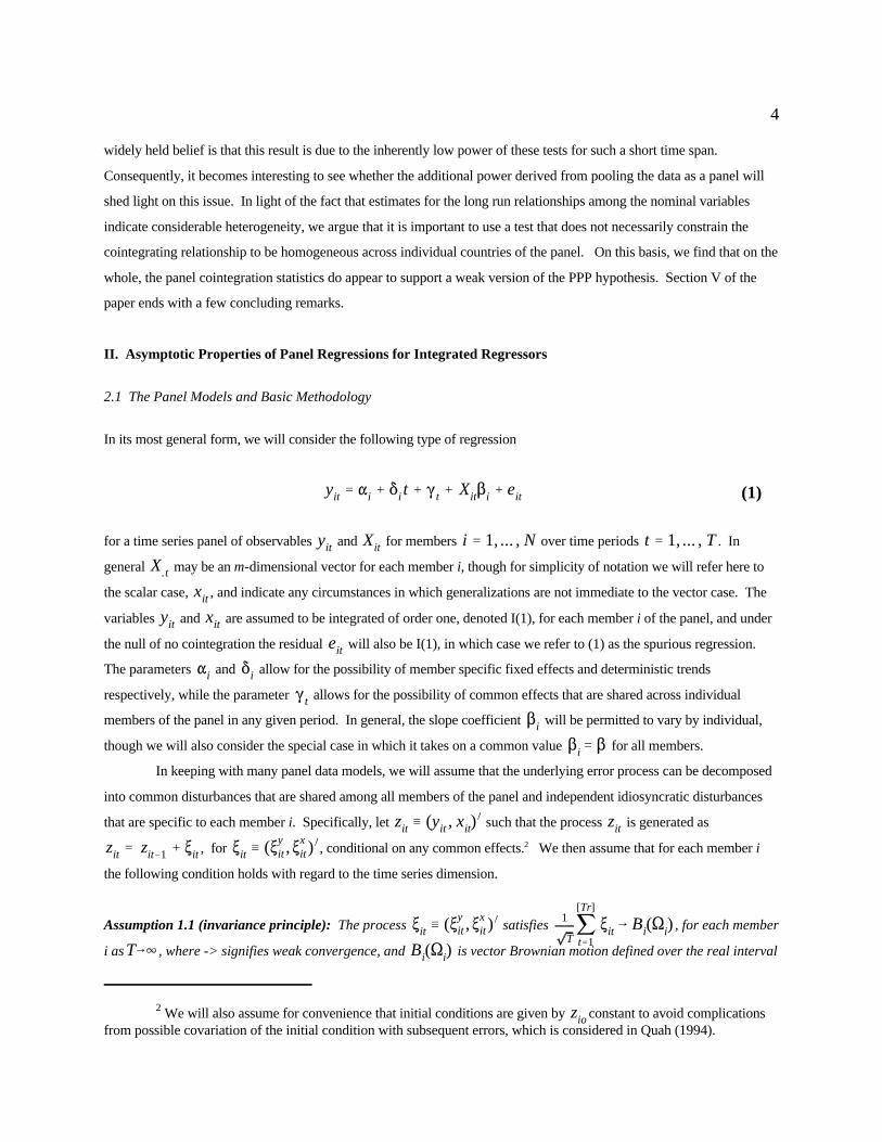
In its most general form, we will consider the following type of regression

for a time series panel of observables and for members over time periods . In

general may be an m-dimensional vector for each member i, though for simplicity of notation we will refer here to

the scalar case, , and indicate any circumstances in which generalizations are not immediate to the vector case. The

variables and are assumed to be integrated of order one, denoted I(1), for each member i of the panel, and under

the null of no cointegration the residual will also be I(1), in which case we refer to (1) as the spurious regression.

The parameters and allow for the possibility of member specific fixed effects and deterministic trends

respectively, while the parameter allows for the possibility of common effects that are shared across individual

members of the panel in any given period. In general, the slope coefficient will be permitted to vary by individual,

though we will also consider the special case in which it takes on a common value for all members.

In keeping with many panel data models, we will assume that the underlying error process can be decomposed

into common disturbances that are shared among all members of the panel and independent idiosyncratic disturbances

that are specific to each member i. Specifically, let such that the process is generated as

, for , conditional on any common effects. We then assume that for each member i2

the following condition holds with regard to the time series dimension.

Assumption 1.1 (invariance principle): The process satisfies , for each member

i as , where -> signifies weak convergence, and is vector Brownian motion defined over the real interval

Si / Soi % 'i % ')

i

where Soi / T &1j

T

t'1>it>

)

it , 'i / T &1jki

s'1ws kij

T

t'1>it>

)

it&s

r, [0,1] Si

Si Si / limT64 E [T &1('Tt'1>it) ('T

t'1>)

it)]

Si / Soi % 'i % ')

i Soi

>it 'i >it

Si

xit Si

"i , *i , $i

Si

'i

wsk >it Zit ' Di Zi t&1 % >it

wsk i' 1& s

k i% 1

>it Si

5

See standard references, eg. Phillips (1986,1987), Phillips and Durlauf (1986), for further discussion of the3

conditions under which assumption 1.1 holds more generally.

(2)

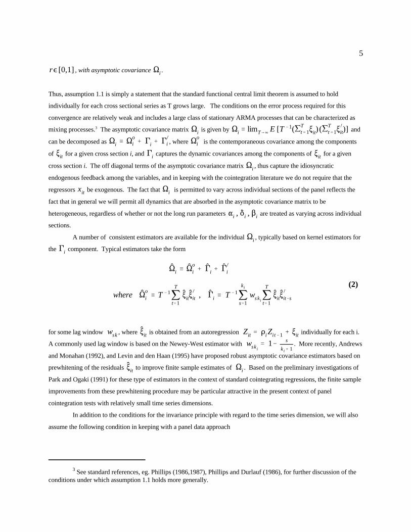
, with asymptotic covariance .

Thus, assumption 1.1 is simply a statement that the standard functional central limit theorem is assumed to hold

individually for each cross sectional series as T grows large. The conditions on the error process required for this

convergence are relatively weak and includes a large class of stationary ARMA processes that can be characterized as

mixing processes. The asymptotic covariance matrix is given by and3

can be decomposed as , where is the contemporaneous covariance among the components

of for a given cross section i, and captures the dynamic covariances among the components of for a given

cross section i. The off diagonal terms of the asymptotic covariance matrix , thus capture the idiosyncratic

endogenous feedback among the variables, and in keeping with the cointegration literature we do not require that the

regressors be exogenous. The fact that is permitted to vary across individual sections of the panel reflects the

fact that in general we will permit all dynamics that are absorbed in the asymptotic covariance matrix to be

heterogeneous, regardless of whether or not the long run parameters are treated as varying across individual

sections.

A number of consistent estimators are available for the individual , typically based on kernel estimators for

the component. Typical estimators take the form

for some lag window , where is obtained from an autoregression individually for each i.

A commonly used lag window is based on the Newey-West estimator with . More recently, Andrews

and Monahan (1992), and Levin and den Haan (1995) have proposed robust asymptotic covariance estimators based on

prewhitening of the residuals to improve finite sample estimates of . Based on the preliminary investigations of

Park and Ogaki (1991) for these type of estimators in the context of standard cointegrating regressions, the finite sample

improvements from these prewhitening procedure may be particular attractive in the present context of panel

cointegration tests with relatively small time series dimensions.

In addition to the conditions for the invariance principle with regard to the time series dimension, we will also

assume the following condition in keeping with a panel data approach

T &1 jT

t' 1Zit&1>

)

it 6 Lim1

0Zi(r) dZi(r))dr Li % 'i

T &2 jT

t' 1

Zit&1 Z )

it&1 6 Lim1

0Zi(r) Zi(r))dr Li

L11i' (S11i& S221i/S22i)

1/2 , L12i' 0 , L21i' S21i/S1/222i , L22i' S1/2

22i

E [>it>)

jt]' 0 for all i…j

IN q Si > 0

Zi(r) / ( Vi(r) , Wi(r) ))

'i Li Si

6

In contrast to the common time dummies, the presence of stochastic cointegrating relationship between4

members will generally impact the limiting distributions if not properly accommodated.

(3b)

(3a)

(4)

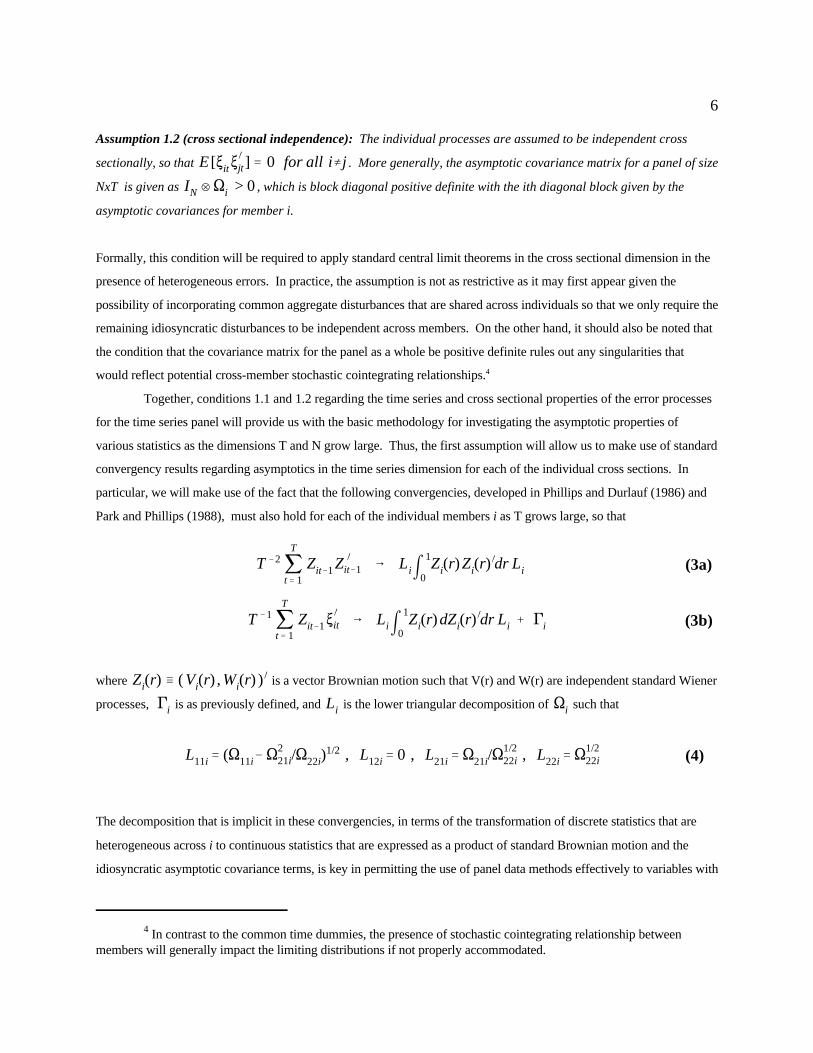
Assumption 1.2 (cross sectional independence): The individual processes are assumed to be independent cross

sectionally, so that . More generally, the asymptotic covariance matrix for a panel of size

NxT is given as , which is block diagonal positive definite with the ith diagonal block given by the

asymptotic covariances for member i.

Formally, this condition will be required to apply standard central limit theorems in the cross sectional dimension in the

presence of heterogeneous errors. In practice, the assumption is not as restrictive as it may first appear given the

possibility of incorporating common aggregate disturbances that are shared across individuals so that we only require the

remaining idiosyncratic disturbances to be independent across members. On the other hand, it should also be noted that

the condition that the covariance matrix for the panel as a whole be positive definite rules out any singularities that

would reflect potential cross-member stochastic cointegrating relationships. 4

Together, conditions 1.1 and 1.2 regarding the time series and cross sectional properties of the error processes

for the time series panel will provide us with the basic methodology for investigating the asymptotic properties of

various statistics as the dimensions T and N grow large. Thus, the first assumption will allow us to make use of standard

convergency results regarding asymptotics in the time series dimension for each of the individual cross sections. In

particular, we will make use of the fact that the following convergencies, developed in Phillips and Durlauf (1986) and

Park and Phillips (1988), must also hold for each of the individual members i as T grows large, so that

where is a vector Brownian motion such that V(r) and W(r) are independent standard Wiener

processes, is as previously defined, and is the lower triangular decomposition of such that

The decomposition that is implicit in these convergencies, in terms of the transformation of discrete statistics that are

heterogeneous across i to continuous statistics that are expressed as a product of standard Brownian motion and the

idiosyncratic asymptotic covariance terms, is key in permitting the use of panel data methods effectively to variables with

Zi(r)

Zi(r)

T64 N64

T64

N64

T64

T64

N64

T64

7

One fairly simple situation in which the iterative convergence condition can be relaxed in a fairly5

straightforward manner is when the original error process is taken to be identical among individual members, since inthis case we do not necessarily require prior application of T dimensional asymptotics to ensure that the statistics will bei.i.d. in the N dimension.

such general and heterogeneous error processes. In particular, the fact that the elements of are standard implies

that the distributions of functionals of will be identical across individual i so that more standard central limit

theorems can be applied to sums of these standardized Brownian motion functionals as N grows large. In this case,

when taking limits sequentially with respect to T and then N, the resulting distributions will be asymptotically normal

and free of nuisance parameters with moments determined solely by the properties of the Brownian motion functionals,

as we will see.

In particular, it should be noted that in formulating these arguments we are in effect applying sequential limit

arguments. By allowing the time series dimension, T, to grow large first, before applying N dimensional asymptotics,

we ensure by virtue of functional central limit theorem arguments that the random variables indexed by i are both

independent and identical since they can be made asymptotically free of idiosyncratic nuisance parameters as T grows

large. We view the restriction that first and then as a relatively strong restriction that ensures these

conditions, and it is possible that in many circumstances a weaker set of restrictions that allow N and T to grow large

concurrently, but with restrictions on the relative rates of growth will deliver similar results. In general, for

heterogeneous error processes, such restrictions on the rate of growth of N relative to T can be expected to depend on

the rate of convergence of the particular kernel estimators used to eliminate the nuisance parameters in addition to the

rate of convergence required by the functional central limit theorem and we can expect that our iterative and5

then requirements proxy for the fact that in practice our asymptotic approximations will be more accurate in

panels with relatively large T dimensions as compared to the N dimension.

Alternatively, under a more pragmatic interpretation that will be appropriate for section 2.3 in which we study

panels with heterogeneous slope coefficients, one can simply think of letting for fixed N reflect the fact that

typically for the panels in which we are interested, it is the time series dimension which can be expected to grow in

actuality rather than the cross sectional dimension, which is in practice fixed. Thus, is in a sense the true

asymptotic feature in which we are interested, and this leads to statistics which are characterized as sums of i.i.d.

Brownian motion functionals. For practical purposes, however, we would like to be able to characterize these statistics

for the general case in which N is large, and in this case we take as a convenient benchmark for which to

characterize the distribution, provided that we understand to be the dominant asymptotic feature of the data.

2.2 Properties of Spurious Regressions and Residual Based Tests in Homogeneous Panels

In order to better understand the issues involved in constructing residual based tests for the null of no cointegration in the

general case in which we allow full heterogeneity of the associated dynamics and long run relationships among

N jN

i'1j

T

t'1

L &222 i x 2

it

&1

jN

i'1j

T

t'1

(L11 iL22 i)&1 xityit&

L21 i

L11 i

x 2it 6 N( 0 , 2/3)

yit xit

"i ' *i ' (t ' 0 $i ' $

T64 N64 Li

T 2

jNi'1 L &2

22i T &2jTt'1 Zit&1Z

)

it&1 22

jNi'1 [m

1

r'0W 2

i (r)dr ]

8

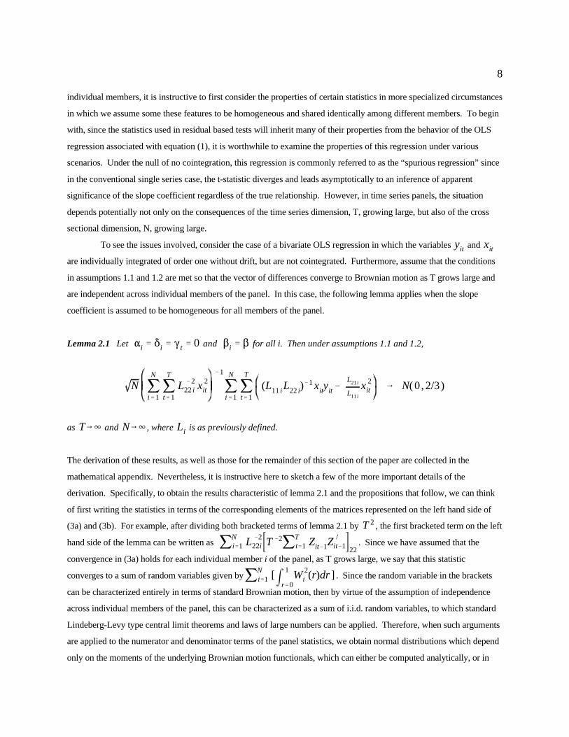
individual members, it is instructive to first consider the properties of certain statistics in more specialized circumstances

in which we assume some these features to be homogeneous and shared identically among different members. To begin

with, since the statistics used in residual based tests will inherit many of their properties from the behavior of the OLS

regression associated with equation (1), it is worthwhile to examine the properties of this regression under various

scenarios. Under the null of no cointegration, this regression is commonly referred to as the “spurious regression” since

in the conventional single series case, the t-statistic diverges and leads asymptotically to an inference of apparent

significance of the slope coefficient regardless of the true relationship. However, in time series panels, the situation

depends potentially not only on the consequences of the time series dimension, T, growing large, but also of the cross

sectional dimension, N, growing large.

To see the issues involved, consider the case of a bivariate OLS regression in which the variables and

are individually integrated of order one without drift, but are not cointegrated. Furthermore, assume that the conditions

in assumptions 1.1 and 1.2 are met so that the vector of differences converge to Brownian motion as T grows large and

are independent across individual members of the panel. In this case, the following lemma applies when the slope

coefficient is assumed to be homogeneous for all members of the panel.

Lemma 2.1 Let and for all i. Then under assumptions 1.1 and 1.2,

as and , where is as previously defined.

The derivation of these results, as well as those for the remainder of this section of the paper are collected in the

mathematical appendix. Nevertheless, it is instructive here to sketch a few of the more important details of the

derivation. Specifically, to obtain the results characteristic of lemma 2.1 and the propositions that follow, we can think

of first writing the statistics in terms of the corresponding elements of the matrices represented on the left hand side of

(3a) and (3b). For example, after dividing both bracketed terms of lemma 2.1 by , the first bracketed term on the left

hand side of the lemma can be written as . Since we have assumed that the

convergence in (3a) holds for each individual member i of the panel, as T grows large, we say that this statistic

converges to a sum of random variables given by . Since the random variable in the brackets

can be characterized entirely in terms of standard Brownian motion, then by virtue of the assumption of independence

across individual members of the panel, this can be characterized as a sum of i.i.d. random variables, to which standard

Lindeberg-Levy type central limit theorems and laws of large numbers can be applied. Therefore, when such arguments

are applied to the numerator and denominator terms of the panel statistics, we obtain normal distributions which depend

only on the moments of the underlying Brownian motion functionals, which can either be computed analytically, or in

3

2N $NT 6 N (0 , S2

11/S222 )

LiL21i

L11i

x 2it

L21' 0

Si ' S S21' 0 $NT

T64 N64

N

$

T &1/2 t$NT6 N( 0,2/3) T64 N64

9

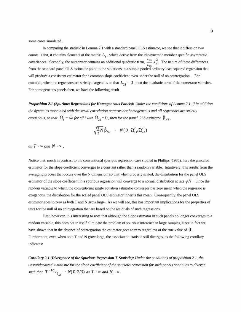
some cases simulated.

In comparing the statistic in Lemma 2.1 with a standard panel OLS estimator, we see that it differs on two

counts. First, it contains elements of the matrix , which derive from the idiosyncratic member specific asymptotic

covariances. Secondly, the numerator contains an additional quadratic term, . The nature of these differences

from the standard panel OLS estimator point to the situations in a simple pooled ordinary least squared regression that

will produce a consistent estimator for a common slope coefficient even under the null of no cointegration. For

example, when the regressors are strictly exogenous so that , then the quadratic term of the numerator vanishes.

For homogeneous panels then, we have the following result

Proposition 2.1 (Spurious Regressions for Homogeneous Panels): Under the conditions of Lemma 2.1, if in addition

the dynamics associated with the serial correlation patterns are homogeneous and all regressors are strictly

exogenous, so that for all i with , then for the panel OLS estimator ,

as and .

Notice that, much in contrast to the conventional spurious regression case studied in Phillips (1986), here the unscaled

estimator for the slope coefficient converges to a constant rather than a random variable. Intuitively, this results from the

averaging process that occurs over the N dimension, so that when properly scaled, the distribution for the panel OLS

estimator of the slope coefficient in a spurious regression will converge to a normal distribution at rate . Since the

random variable to which the conventional single equation estimator converges has zero mean when the regressor is

exogenous, the distribution for the scaled panel OLS estimator inherits this mean. Consequently, the panel OLS

estimator goes to zero as both T and N grow large. As we will see, this has important implications for the properties of

tests for the null of no cointegration that are based on the residuals of such regressions.

First, however, it is interesting to note that although the slope estimator in such panels no longer converges to a

random variable, this does not in itself eliminate the problem of spurious inference in large samples, since in fact we

have shown that in the absence of cointegration the estimator goes to zero regardless of the true value of .

Furthermore, even when both T and N grow large, the associated t-statistic still diverges, as the following corollary

indicates:

Corollary 2.1 (Divergence of the Spurious Regression T-Statistic): Under the conditions of proposition 2.1, the

unstandardized t-statistic for the slope coefficient of the spurious regression for such panels continues to diverge

such that as and .

T N(DNT & 1) / T N jN

i'1j

T

t'1e 2

it&1

&1

jN

i'1j

T

t'1eit&1)eit & 8i 6 N( 0 , 2)

tDNT/ F2

NT jN

i'1j

T

t'1

e 2it&1

&1/2

jN

i'1j

T

t'1

eit&1)eit & 8i 6 N( 0 , 1)

T64 N64 8i ' T &1jki

s'1

ws kijT

t'1

µ itµ it&s wsk it

$

10

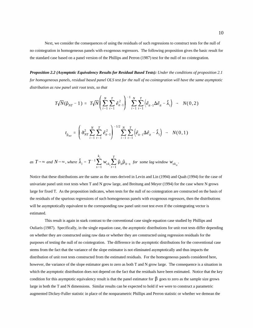
Next, we consider the consequences of using the residuals of such regressions to construct tests for the null of

no cointegration in homogeneous panels with exogenous regressors. The following proposition gives the basic result for

the standard case based on a panel version of the Phillips and Perron (1987) test for the null of no cointegration.

Proposition 2.2 (Asymptotic Equivalency Results for Residual Based Tests): Under the conditions of proposition 2.1

for homogeneous panels, residual based panel OLS test for the null of no cointegration will have the same asymptotic

distribution as raw panel unit root tests, so that

as and , where for some lag window .

Notice that these distributions are the same as the ones derived in Levin and Lin (1994) and Quah (1994) for the case of

univariate panel unit root tests when T and N grow large, and Breitung and Meyer (1994) for the case where N grows

large for fixed T. As the proposition indicates, when tests for the null of no cointegration are constructed on the basis of

the residuals of the spurious regressions of such homogeneous panels with exogenous regressors, then the distributions

will be asymptotically equivalent to the corresponding raw panel unit root test even if the cointegrating vector is

estimated.

This result is again in stark contrast to the conventional case single equation case studied by Phillips and

Ouliaris (1987). Specifically, in the single equation case, the asymptotic distributions for unit root tests differ depending

on whether they are constructed using raw data or whether they are constructed using regression residuals for the

purposes of testing the null of no cointegration. The difference in the asymptotic distributions for the conventional case

stems from the fact that the variance of the slope estimator is not eliminated asymptotically and thus impacts the

distribution of unit root tests constructed from the estimated residuals. For the homogeneous panels considered here,

however, the variance of the slope estimator goes to zero as both T and N grow large. The consequence is a situation in

which the asymptotic distribution does not depend on the fact that the residuals have been estimated. Notice that the key

condition for this asymptotic equivalency result is that the panel estimator for goes to zero as the sample size grows

large in both the T and N dimensions. Similar results can be expected to hold if we were to construct a parametric

augmented Dickey-Fuller statistic in place of the nonparametric Phillips and Perron statistic or whether we demean the

)Zit ' >it Si>it

$

>it >it

Si

Si

11

In subsequent work, we also consider the case in which heterogeneity is present in the dynamics and the6

endogeneity of the regressors, but the assumption of homogeneity of the slope coefficient is maintained.

Alternatively, one can difference the original data to obtain and then estimate on the basis of7

these values of . However the estimators are no longer consistent against certain alternates in this case. See Phillipsand Ouliaris (1990) for a discussion of these issues.

series by estimating an intercept. The distributions for unit root tests constructed from the estimated residuals of such

regressions will have the same distribution of the corresponding raw unit root tests provided that slope coefficient is

homogeneous and the regressors are exogenous. Tables IB and IIB of the appendix illustrate the extent to which

proposition 2.1 and its corollary and proposition 2.2 hold in small samples for various dimensions of N and T based on

Monte Carlo simulation for i.i.d. errors. In the next section we study the properties of residual based tests for the null of

no cointegration when the assumption of homogeneity does not apply and propose a set of statistics designed to deal with

this case.

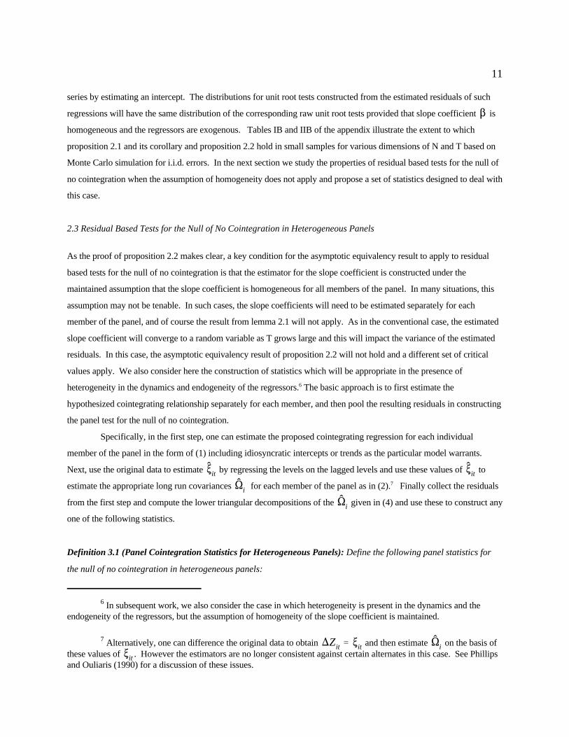
2.3 Residual Based Tests for the Null of No Cointegration in Heterogeneous Panels

As the proof of proposition 2.2 makes clear, a key condition for the asymptotic equivalency result to apply to residual

based tests for the null of no cointegration is that the estimator for the slope coefficient is constructed under the

maintained assumption that the slope coefficient is homogeneous for all members of the panel. In many situations, this

assumption may not be tenable. In such cases, the slope coefficients will need to be estimated separately for each

member of the panel, and of course the result from lemma 2.1 will not apply. As in the conventional case, the estimated

slope coefficient will converge to a random variable as T grows large and this will impact the variance of the estimated

residuals. In this case, the asymptotic equivalency result of proposition 2.2 will not hold and a different set of critical

values apply. We also consider here the construction of statistics which will be appropriate in the presence of

heterogeneity in the dynamics and endogeneity of the regressors. The basic approach is to first estimate the6

hypothesized cointegrating relationship separately for each member, and then pool the resulting residuals in constructing

the panel test for the null of no cointegration.

Specifically, in the first step, one can estimate the proposed cointegrating regression for each individual

member of the panel in the form of (1) including idiosyncratic intercepts or trends as the particular model warrants.

Next, use the original data to estimate by regressing the levels on the lagged levels and use these values of to

estimate the appropriate long run covariances for each member of the panel as in (2). Finally collect the residuals7

from the first step and compute the lower triangular decompositions of the given in (4) and use these to construct any

one of the following statistics.

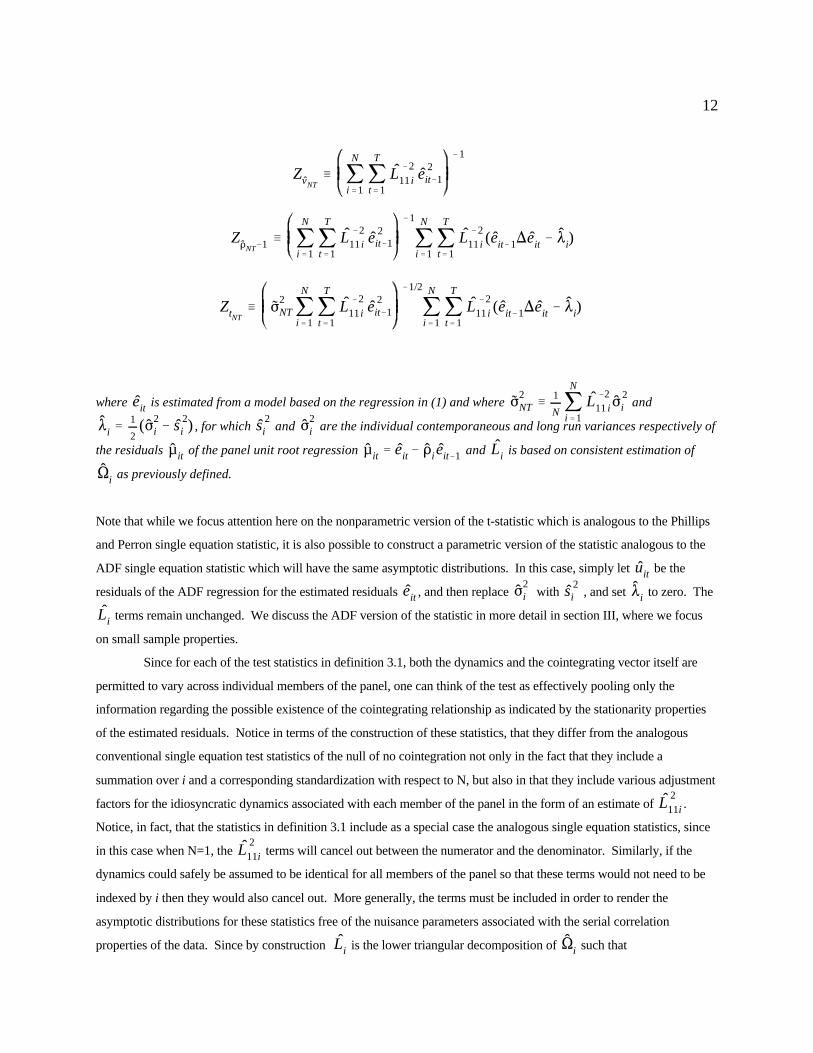
Definition 3.1 (Panel Cointegration Statistics for Heterogeneous Panels): Define the following panel statistics for

the null of no cointegration in heterogeneous panels:

ZvNT/ j

N

i'1j

T

t'1L

&211 i e 2

it&1

&1

ZDNT&1 / jN

i'1j

T

t'1L

&211 i e 2

it&1

&1

jN

i'1j

T

t'1L

&211 i (eit&1)eit & 8i)

ZtNT/ F2

NT jN

i'1j

T

t'1L

&211 i e 2

it&1

&1/2

jN

i'1j

T

t'1L

&211 i (eit&1)eit & 8i)

eit F2NT / 1

N jN

i'1

L&211 i F

2i

8i '1

2(F2

i & s 2i ) s 2

i F2i

µ it µ it ' eit& Di eit&1 Li

Si

uit

eit F2i s 2

i 8i

Li

L211i

L211i

Li Si

12

where is estimated from a model based on the regression in (1) and where and

, for which and are the individual contemporaneous and long run variances respectively of

the residuals of the panel unit root regression and is based on consistent estimation of

as previously defined.

Note that while we focus attention here on the nonparametric version of the t-statistic which is analogous to the Phillips

and Perron single equation statistic, it is also possible to construct a parametric version of the statistic analogous to the

ADF single equation statistic which will have the same asymptotic distributions. In this case, simply let be the

residuals of the ADF regression for the estimated residuals , and then replace with , and set to zero. The

terms remain unchanged. We discuss the ADF version of the statistic in more detail in section III, where we focus

on small sample properties.

Since for each of the test statistics in definition 3.1, both the dynamics and the cointegrating vector itself are

permitted to vary across individual members of the panel, one can think of the test as effectively pooling only the

information regarding the possible existence of the cointegrating relationship as indicated by the stationarity properties

of the estimated residuals. Notice in terms of the construction of these statistics, that they differ from the analogous

conventional single equation test statistics of the null of no cointegration not only in the fact that they include a

summation over i and a corresponding standardization with respect to N, but also in that they include various adjustment

factors for the idiosyncratic dynamics associated with each member of the panel in the form of an estimate of .

Notice, in fact, that the statistics in definition 3.1 include as a special case the analogous single equation statistics, since

in this case when N=1, the terms will cancel out between the numerator and the denominator. Similarly, if the

dynamics could safely be assumed to be identical for all members of the panel so that these terms would not need to be

indexed by i then they would also cancel out. More generally, the terms must be included in order to render the

asymptotic distributions for these statistics free of the nuisance parameters associated with the serial correlation

properties of the data. Since by construction is the lower triangular decomposition of such that

T N ZDNT&1 & 121&11 N 6 N( 0, N)

(2)R(2)N(2) )

ZtNT& 12 (11(1%13))

&1/2 N 6 N (0, N)

(3)R(3)N(3) )

T 2 N 3/2 ZvNT& 1&1

1 N 6 N( 0, N)

(1)R(1)N(1) )

L211 i ' T11 i &

T221 i

T22 i

1 R

1 R

1, RK) / (mQ 2,mQdQ, $2

) $ / mVW

mW2Q / V& $W R(j)

R

N(j) N)

(1) ' & 1&21 N)

(2) ' & (1&11 ,121

&21 )

N)

(3) ' (1&1/21 (1%13)

&1/2, & 1

2121

&3/21 (1%13)

&1/2, & 1

2121

&1/21 (1%13)

&3/2 )

T64

13

, the term can be interpreted more specifically as the asymptotic conditional variance for the

initial regression associated with (1).

For the following proposition, we posit and respectively to be finite mean and covariances of the

appropriate vector Brownian motion functional. As the following proposition indicates, when the statistics are

constructed in the manner of definition 3.1 and standardized by the appropriate values for N and T, then the asymptotic

distributions will depend only on known parameters given by and .

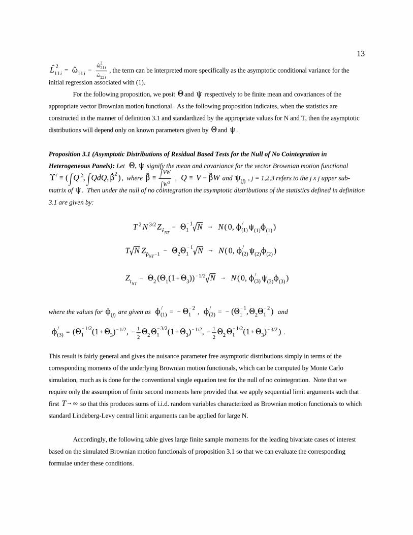
Proposition 3.1 (Asymptotic Distributions of Residual Based Tests for the Null of No Cointegration in

Heterogeneous Panels): Let signify the mean and covariance for the vector Brownian motion functional

, where , and , j = 1,2,3 refers to the j x j upper sub-

matrix of . Then under the null of no cointegration the asymptotic distributions of the statistics defined in definition

3.1 are given by:

where the values for are given as , and

.

This result is fairly general and gives the nuisance parameter free asymptotic distributions simply in terms of the

corresponding moments of the underlying Brownian motion functionals, which can be computed by Monte Carlo

simulation, much as is done for the conventional single equation test for the null of no cointegration. Note that we

require only the assumption of finite second moments here provided that we apply sequential limit arguments such that

first so that this produces sums of i.i.d. random variables characterized as Brownian motion functionals to which

standard Lindeberg-Levy central limit arguments can be applied for large N.

Accordingly, the following table gives large finite sample moments for the leading bivariate cases of interest

based on the simulated Brownian motion functionals of proposition 3.1 so that we can evaluate the corresponding

formulae under these conditions.

1 , RK) / (mQ 2,mQdQ, $2

) $ / mVW

mW2Q / V& $W 1) , R) 1)) , R))

V ),W ) V )),W ))

1 '

0.250

&0.693

0.889

R'

0.110

&0.011 0.788

0.243 &1.326 3.174

1) '

0.116

&0.698

0.397

R) '

0.011

&0.013 0.179

0.026 &0.238 0.480

1)) '

0.056

&0.590

0.182

R)) '

0.001

&0.001 0.034

0.003 &0.042 0.085

Z , Z ) , Z ))

N64

T 2 N 3/2 ZvNT& 4.00 N 6 N (0, 27.81)

T 2 N 3/2 Z )

vNT& 8.62 N 6 N (0, 60.75)

T 2 N 3/2 Z ))

vNT& 17.86 N 6 N (0, 101.68)

14

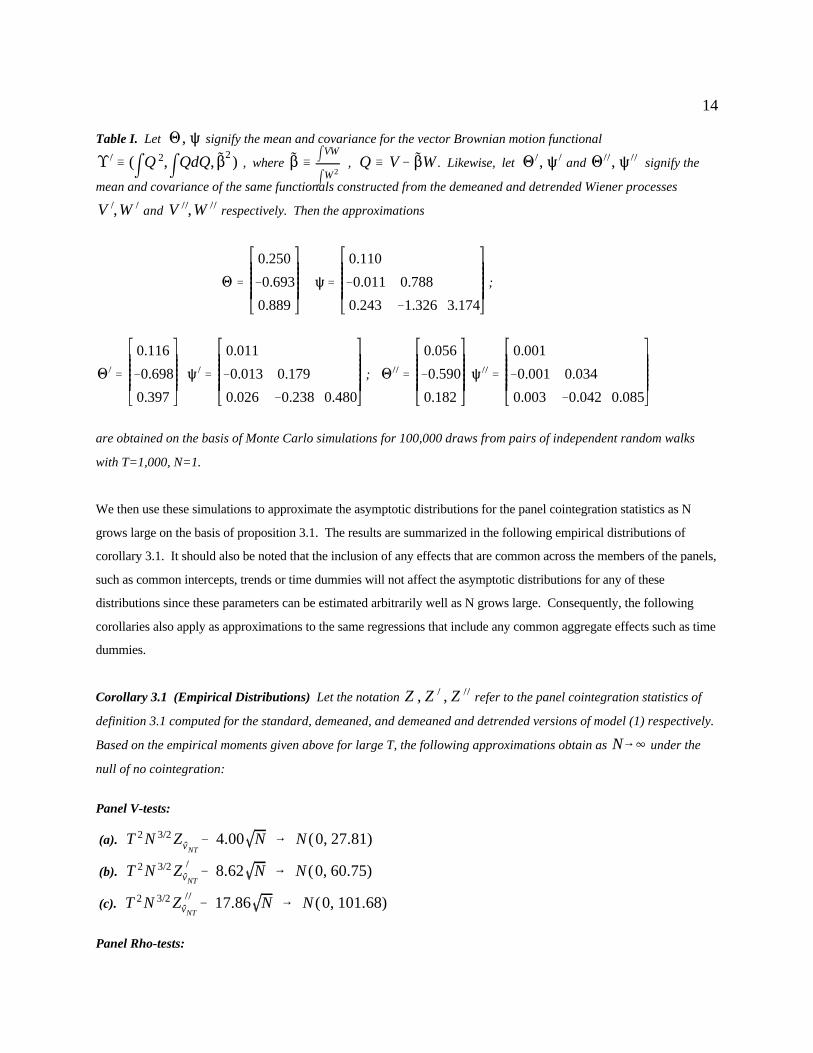
Table I. Let signify the mean and covariance for the vector Brownian motion functional

, where , . Likewise, let and signify the

mean and covariance of the same functionals constructed from the demeaned and detrended Wiener processes

and respectively. Then the approximations

;

;

are obtained on the basis of Monte Carlo simulations for 100,000 draws from pairs of independent random walks

with T=1,000, N=1.

We then use these simulations to approximate the asymptotic distributions for the panel cointegration statistics as N

grows large on the basis of proposition 3.1. The results are summarized in the following empirical distributions of

corollary 3.1. It should also be noted that the inclusion of any effects that are common across the members of the panels,

such as common intercepts, trends or time dummies will not affect the asymptotic distributions for any of these

distributions since these parameters can be estimated arbitrarily well as N grows large. Consequently, the following

corollaries also apply as approximations to the same regressions that include any common aggregate effects such as time

dummies.

Corollary 3.1 (Empirical Distributions) Let the notation refer to the panel cointegration statistics of

definition 3.1 computed for the standard, demeaned, and demeaned and detrended versions of model (1) respectively.

Based on the empirical moments given above for large T, the following approximations obtain as under the

null of no cointegration:

Panel V-tests:

(a).

(b).

(c).

Panel Rho-tests:

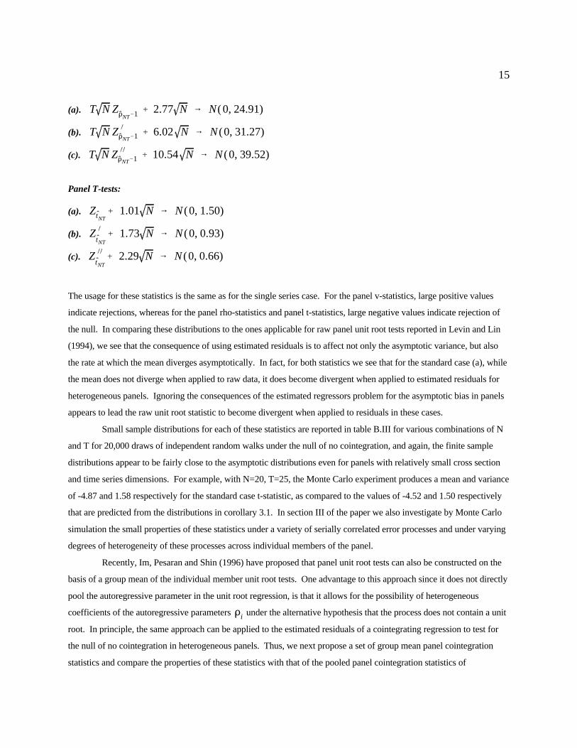
T N ZDNT&1 % 2.77 N 6 N( 0, 24.91)

T N Z )

DNT&1 % 6.02 N 6 N (0, 31.27)

T N Z ))

DNT&1 % 10.54 N 6 N (0, 39.52)

ZtNT% 1.01 N 6 N (0, 1.50)

Z )

tNT% 1.73 N 6 N (0, 0.93)

Z ))

tNT% 2.29 N 6 N (0, 0.66)

Di

15

(a).

(b).

(c).

Panel T-tests:

(a).

(b).

(c).

The usage for these statistics is the same as for the single series case. For the panel v-statistics, large positive values

indicate rejections, whereas for the panel rho-statistics and panel t-statistics, large negative values indicate rejection of

the null. In comparing these distributions to the ones applicable for raw panel unit root tests reported in Levin and Lin

(1994), we see that the consequence of using estimated residuals is to affect not only the asymptotic variance, but also

the rate at which the mean diverges asymptotically. In fact, for both statistics we see that for the standard case (a), while

the mean does not diverge when applied to raw data, it does become divergent when applied to estimated residuals for

heterogeneous panels. Ignoring the consequences of the estimated regressors problem for the asymptotic bias in panels

appears to lead the raw unit root statistic to become divergent when applied to residuals in these cases.

Small sample distributions for each of these statistics are reported in table B.III for various combinations of N

and T for 20,000 draws of independent random walks under the null of no cointegration, and again, the finite sample

distributions appear to be fairly close to the asymptotic distributions even for panels with relatively small cross section

and time series dimensions. For example, with N=20, T=25, the Monte Carlo experiment produces a mean and variance

of -4.87 and 1.58 respectively for the standard case t-statistic, as compared to the values of -4.52 and 1.50 respectively

that are predicted from the distributions in corollary 3.1. In section III of the paper we also investigate by Monte Carlo

simulation the small properties of these statistics under a variety of serially correlated error processes and under varying

degrees of heterogeneity of these processes across individual members of the panel.

Recently, Im, Pesaran and Shin (1996) have proposed that panel unit root tests can also be constructed on the

basis of a group mean of the individual member unit root tests. One advantage to this approach since it does not directly

pool the autoregressive parameter in the unit root regression, is that it allows for the possibility of heterogeneous

coefficients of the autoregressive parameters under the alternative hypothesis that the process does not contain a unit

root. In principle, the same approach can be applied to the estimated residuals of a cointegrating regression to test for

the null of no cointegration in heterogeneous panels. Thus, we next propose a set of group mean panel cointegration

statistics and compare the properties of these statistics with that of the pooled panel cointegration statistics of

ZtNT/ j

N

i'1j

T

t'1

L&211 i e 2

it&1

&1/2

jT

t'1

(eit&1)eit & 8i)

ZDNT&1 / jN

i'1j

T

t'1e 2

it&1

&1

jT

t'1(eit&1)eit & 8i)

N &1/2 ZtNT& 12 N 6 N (0 , R2,2 )

TN &1/2 ZDNT&1 & 11 N 6 N (0 , R1,1 )

eit 8i '1

2(F2

i & s 2i ) s 2

i

F2i µ it

µ it ' eit& Di eit&1 Li Si

1, RK) / (mQ 2)&1mQdQ , ((1& $2

)mQ 2)&1/2mQdQ $ / mVW

mW2Q / V& $W

1, R

16

proposition 3.1 and its corollary.

Definition 3.2 (Group Mean Panel Cointegration Statistics for Heterogeneous Panels): Define the following group

mean panel statistics for the null of no cointegration in heterogeneous panels:

where is estimated from a model based on the regression in (1) and where , for which and

are the individual contemporaneous and long run variances respectively of the residuals of the panel unit

root regression and is based on consistent estimation of as previously defined.

In principle it is also possible to construct a group mean panel variance ratio statistic analogous to the one presented for

the pooled panel cointegration statistics in definition 3.1. But given the relatively poorer performance of variance ratio

statistics in the conventional single equation case, since the group mean approach essentially amounts to averaging the

single equation statistics for each member of the panel, we restrict our attention here to the group mean panel rho- and t-

statistics. The following proposition presents the general result, which we again follow with empirical distributions for

the leading bivariate case.

Proposition 3.2 (Asymptotic Distributions of Residual Based Group Mean Tests for the Null of No Cointegration in

Heterogeneous Panels): Let signify the mean and variance for the vector Brownian motion functional

, where , and . Then under the

null of no cointegration the asymptotic distributions of the statistics defined in definition 3.2 are given by:

where the subscripts on the matrices refer to the corresponding elements.

1 , RK) / (mQ 2)&1mQdQ , ((1& $2

)mQ 2)&1/2mQdQ $ / mVW

mW2Q / V& $W

1), R) 1))

, R))

V ) , W ) V )),W ))

1 '&6.836

&1.389Diag (R) '

26.782

0.781

1)'

&9.049

&2.025Diag (R) ) '

35.976

0.6601))

'&13.649

&2.528Diag (R)) ) '

50.907

0.561

Z , Z), Z

))

N64

TN &1/2 ZDNT&1 % 6.84 N 6 N( 0, 26.78)

TN &1/2 Z)

DNT&1 % 9.05 N 6 N( 0, 35.98)

TN &1/2 Z))

DNT&1 % 13.65 N 6 N( 0, 50.91)

N &1/2 ZtNT% 1.39 N 6 N (0, 0.78)

N &1/2 Z )

tNT% 2.03 N 6 N (0, 0.66)

17

Next, we simulate the moments of the appropriate Brownian motion functionals and report these in the following table

for the case of standard, demeaned and detrended processes. Note that the statistics of proposition 3.2 require only the

diagonals of the covariance matrix for the vector of functionals, which we report accordingly.

Table II. Let signify the mean and covariance for the vector Brownian motion functional

, where , . Likewise, let

and signify the mean and covariance of the same functionals constructed from the demeaned and

detrended Wiener processes and respectively. Then the approximations

;

;

are obtained on the basis of Monte Carlo simulations for 100,000 draws from pairs of independent random walks

with T=1,000, N=1.

Thus, the empirical distributions similar in spirit to corollary 3.1 can be obtained simply by substituting the

corresponding empirical moments from Table II into proposition 3.2, which gives the following results.

Corollary 3.2 (Empirical Distributions) Let the notation refer to the panel cointegration statistics of

definition 3.2 computed for the standard, demeaned, and demeaned and detrended versions of model (1) respectively.

Based on the empirical moments given above for large T, the following approximations obtain as under the

null of no cointegration:

Group Mean Panel Rho-tests:

(a).

(b).

(c).

Group Mean Panel T-tests:

(a).

(b).

yit& xit ' v1it ; v1it ' Dv1it&1% w1it

xit ' ayit% v2it ; v2it ' v2it&1% w2it

w2it' Nit% (iNit&1 ; (w1it,Nit)) ~ Ni( (0,0)), Vi )

N &1/2 Z ))

tNT% 2.53 N 6 N (0, 0.56)

ZtNT

yit xit t ' 1,... ,T i ' 1,... ,N

Vi F2i 2iFi

D ' 1

D < 1

a ' 0 xit

18

(c).

The usage for these statistics are the same as for the analogous panel cointegration statistics of corollary 3.1 in that large

negative values indicate rejections of the null of no cointegration. Again, it should be noted that the approximate

asymptotic distributions for the will also apply to an ADF based panel cointegration statistic. We now turn our

attention in the next section to a comparison of the small sample properties of each of these statistics through a series of

Monte Carlo experiments.

III. Monte Carlo Experiments.

In this section we concern ourselves with a study of the small sample size and power properties of the various statistics

proposed in the previous section for testing the null of no cointegration in heterogeneous panels, including also the

parametric ADF versions of the t-statistics. It is well known that conventional single equation tests for the null of no

cointegration tend to suffer from low power in small samples and are also susceptible to fairly large size distortions,

particularly in the presence of MA components in the error processes. Papers by Stock (1990), Kremers, Ericson and

Dolado (1992), and Gonzalo (1994) have studied various aspects of these properties by Monte Carlo simulation. Most

recently, studies by Haug (1993, 1996) provide a systematic overview of both the sample size and power properties of a

number of conventional tests for the null of no cointegration, which we use here to motivate our Monte Carlo

experiments for heterogeneous panels.

In particular, we employ the following panel data version of the data generating process used by Haug (1996).

Specifically, we have

Data Generating Process 4.1: Let , , , be generated by

where is a variance-covariance matrix with diagonals 1, and off-diagonals .

Notice in particular for DGP 4.1, that when , the residuals for the regression of type (1) are nonstationary, so that

the null of no cointegration is true, whereas when the residuals are stationary and the alternate hypothesis of

cointegration is true. Other interesting features to note are that when the regressors, , become exogenous and

(i ' 0 (i … 0

Vi

2i ,Fi

(w1it ,Nit))

( ,2 ,F D

a ' (0,1) 2 ' (&0.5,0.0, 0.5) F' (0.25, 1.0,4.0) ( ' (&0.8,0.0, 0.8)

D ' (1.0,0.9)

( ,2 ,F D ' 1.0

a ' 1

a ' 0

19

when the error process becomes i.i.d. More generally, when , the errors will contain moving average

components, which we will allow to vary according to the individual member of the panel. Similarly, we will also allow

the variance-covariance matrix to vary by individual member in some experiments, by varying the parameters

. Specifically, we model these variations across members by drawing the parameters from a uniform distribution

in a manner that allows for considerable heterogeneity in the associated dynamics. For each of the experiments that we

consider, we draw these parameters once at the beginning of the experiment in order to fix them for each member of the

panel, and then produce independent draws of the vector to generate 2000 realizations of the corresponding

panel data set described above. We then repeat these experiments for various values for the parameters of interest, such

as N, T, a, and that impact the small sample size and power properties of the data.

Initially for ease of comparison with more conventional single equation techniques, we compare the properties

of these statistics under a variety of parameterizations of the DGP in 4.1 for the case in which the parameters do not vary

by cross sectional member of the panel. Thus, following Haug (1996) we investigated the following parameter

combinations , , , and

for various combinations of N and T. Following Haug, Table 1 reports results for T=100. We also

report results for T=20 in Table 2 and T=250 in Table 3, since in addition to providing reasonable variations for this

dimension, these values for T represent approximately the sample sizes for the annual and monthly data respectively that

we use for the purchasing power parity example in the next section. By this same reasoning, we report results for the

case where N=20, since this is a reasonable number for a relatively small panel, and also represents approximately the

dimensionality of the panel data set that we employ in the example of the next section. Specifically Tables 1 through 3

report empirical sizes for each of the seven panel cointegration statistics developed in the previous section under DGP

4.1 for various values of with a nominal size of 5% under the null of no cointegration when and for

the case of endogeneity of the regressors, so that . For the purposes of the Monte Carlo simulations, the value for

the lag truncations in the ADF and for the bandwidth of the Newey-West estimator for the nonparametric statistics was

set to a fixed value of K=1 when T=20, K=5 when T=100 and K=7 when T=250 to reflect the presumption that

empirical truncation values will generally be set to larger values in empirical studies with longer data spans.

On the whole, the results of the Monte Carlo simulations for Tables 1 through 3 indicate that the size

distortions for almost all of the proposed panel cointegration statistics are relatively small provided that any moving

average components are positive, with the possible exception of the panel variance statistic, which occasionally has very

small empirical sizes, and the group ADF, which occasionally has somewhat larger empirical sizes than the others. As

expected, the size distortions are generally least for T=250 and greatest for smaller values of T. We also conducted

these experiments for T=50 and also for various combinations with N=50. Since the results were also as expected, with

T=50 lying between T=100 and T=20 and N=50 generally improving on the case where N=20 provided that T was

large, to conserve space we do not include these in the reported tables. Additionally we also ran the simulations for the

case of exogenous regressors by setting . In keeping with Haug, we also found that the distortions were generally

always lower in this case. Since for Tables 1 through 3 the distortions are generally highest when T=20, for this case we

( ' &0.8a ' 0

a ' 0

F ' 1.0 F( ' &0.8

Vi F2i ' 1, 2i ' 0 i

(i U(0,0.4) U(0,0.8) U(&0.4,0.4)

(i

Vi

Fi 2i Fi ~ U(0.25,4) 2i ~ U(&0.5,0.5)

(i (i ' 0 i (i ' 0.8 i

(i Fi 2i (i

(i ~ U(0,0.8)

(i

a'0 a'1

Fi ' 1, 2i'0 (i

U(&0.4,0.4) U(&0.4,0.0) U(&0.4,0.8) U(&0.8,0.8)

(i

20

Notice, by contrast, that in table 4 the size distortions are not large even for since here a has been8

set to for this table. Also, below we will see that the assessment is not quite so extreme in the case where theparameters are allowed to vary over individual members of the panels.

also report separately in Table 4 all of the results for the parameterizations with . Notice of course that we only

report values for , since for the case when regressors are exogenous, the particular value for will not matter

for the regression. Finally, we also experimented with values of . Again, in accordance with the findings of

Haug for the conventional single equation case, this generally leads to very large size distortions for the case of

endogenous regressors, and we do not present these results in tabular form, since they almost uniformly result in the

empirical size going to one. Thus, we conclude that one should continue to exercise caution in the presence of large

negative moving average components in panels just as in conventional single equation case, particularly in the event that

the regressors are not exogenous. 8

Next, in Tables 5 through 7 we report the consequences for the empirical small sample sizes of each of these

proposed panel cointegration statistics when the parameters are allowed to vary across individual members of the panel

as described above. Specifically, in Table 5 we fix the values for by setting for all , and then

drawing the parameter from the following uniform distributions, , and ,

depending on the particular experiment. For the first two cases, all of the statistics perform very well, with the possible

exception of the panel variance and the group rho statistics, which occasionally exhibit empirical sizes which are too

small when T=20, and the group ADF statistic which produces somewhat larger empirical sizes then the others when

T=20 and T=100. For the third case, where the take on both positive and negative values, the group ADF exhibits

fairly large size distortions, for example 0.687 when T=100, while the others remain fairly reasonable, with for example

the panel rho and the panel PP statistics both giving just over 0.15 when T=100.

Proceeding to Table 6, we consider the consequences of allowing to vary across individual members of the

panel by drawing both and from uniform distributions and . In the first

two experiments we fix the values for at for all and for all respectively. In the third

experiment we allow also to vary in addition to and , such that is drawn from the distribution

. In general, for each of these experiments we find that the size distortions tend to be relatively minor,

with the occasional exceptions of the panel v-statistic and the group rho statistic, which take on empirical sizes which

are too low in a few cases, and the group ADF, which occasionally takes on somewhat higher empirical sizes than the

others, particularly when T is small. Finally, Table 7 reports the consequences for the empirical sizes of the various

statistics in relatively small panels, with N=20, T=20 in the event that is allowed to vary over both positive and

negative values in the case of both exogenous and endogenous regressors. Specifically, for both and four

experiments are conducted which fix for all i and allow to vary across individual members of the

panel according to the uniform distributions , , and

respectively. It is interesting to contrast the results of this table with the case in which the values for are the same for

all i and are uniformly negative. As mentioned earlier, in those cases empirical sizes generally always approach unity

(i

(i (i

(i

(i

U(&0.4,0.4) U(&0.4,0.0) U(&0.4,0.8)

(i

U(&0.4,0.4) U(&0.8,0.8)

D'0.85 D'0.9

F2

21

when the regressors are endogenous. However, in the experiments for Table 7, where varies over uniform

distributions that produce some large negative values for but balance these with other values for which are either

positive or negative but close to zero, then we find that the empirical sizes are quite reasonable for some of the statistics,

even when the regressors are endogenous.

Generally speaking, the results appear to show that the more the distribution of is allowed to span large

negative values, the greater will be the empirical size distortions, though these can be further mitigated by the presence

of offsetting positive values in the distribution. Thus, for example, most of the statistics do better when varies over

than when it varies over , but not as well as when it varies over .

However, it is not merely the mean of the distribution which appears to matter, but also the absolute range of negative

values spanned, as can be seen by comparing the better performance of the statistics when varies over

than when it varies over . In comparing the performance of the various statistics, in

general the panel rho statistic does best, while the panel variance and the group ADF do poorest, with the former

consistently producing empirical sizes of zero and the latter producing substantially higher empirical sizes than the

others. While not as extreme as the panel variance statistic, the group rho statistic also tended to produce empirical sizes

which were too low.

The remainder of the tables, 8 through 14, examine the small sample power properties of the panel

cointegration statistics for the same sequence of experiments. Whereas Haug investigates the small sample power

properties for and and reports only the former, we choose here to report the latter case given the

greater power than can be expected in panels. In general, the power is very high when T=100 and T=250, generally

approaching 100% for all cases in Tables 8 and 9. Exceptions are when is small, especially when combined with

negative values for . However, when T=250, even in these situations the power approaches close to 100% except in a

small number of cases for the panel variance statistic in which it does not do well. The situation is not the same when T

becomes as small as T=20. In the case where the regressors are endogenous, as in Table 10, the panel variance statistic

and the group rho statistic do poorly in all cases. The group ADF generally does best, followed by the panel ADF and

panel PP. The panel rho and group PP are reasonable, but generally not quite as good. Table 11 reports power

properties for the case in which the regressors are exogenous for the case when T=20. Tables 12 through 14 report on

the power properties when the parameters of the DGP are allowed to vary for individual members of the panel for the

same set of experiments as described for the size experiments of Tables 5 through 7. Again, the power generally

approaches 100% when T=100 and T=250, but varies when T is as small as T=20.

In summary, the Monte Carlo experiments reported in these tables indicate that the different statistics have

comparative advantages under differing scenarios for the data generating process. While the panel variance statistic is

most easily dominated in the majority of cases, for the other statistics, the relative performance depends very much on

the particular situation and the objective, and there are even a few extreme situations in which the panel variance statistic

performs well relative to others. More generally, in terms of size distortion, it can be said that for the experiments

performed, the panel rho statistic most often exhibited the least distortions among the seven statistics. This was

22

particularly evident in extreme cases when the dimensionality of the panel was small and substantial heterogeneity was

present in the DGP across different members of the panel. Among the seven statistics, the group ADF generally

exhibited the largest empirical size distortions. As compared to the others, the group rho statistic exhibited empirical

sizes that were too low in many cases. The group PP, panel PP and panel ADF generally fell somewhere in between the

group ADF and the panel rho.

In terms of power, with the occasional exception of the panel variance statistic, all other statistics did very well

for panels with reasonably long spans and generally approached close to 100% in all cases with T=100 and larger. For

shorter panels, with T=20, the situation was varied, with the group ADF generally doing best, followed by the panel

ADF and the panel rho. Overall, trading off size and power, the panel rho statistic appears to be the most consistently

reliable statistic, particular in situations with somewhat larger values for T. Of course, one should be aware that these

experiments were all conducted with fixed values for the lag order (which was varied only with the value for sample size

T), and that in general one expects to further improve on these small sample properties in typical empirical work by

implementing data determined lag selection schemes. Alternatively, it may also be possible to further improve on small

sample properties by conditioning on a fixed value for the lag order as suggested in the panel unit root study by Im,

Pesaran and Shin (1995). Finally, it is worthwhile to note that, much in accordance with the findings of Haug’s (1996)

Monte Carlo study for the single equation case, the panel statistics also exhibit considerable size distortions in the

presence of large negative moving average components when these are shared among all members of the panel.

However, in situations where only some members exhibit these characteristics, while others do not, the statistics appear

to perform reasonably well. This may provide another promising advantage to pooling nonstationary data in time series

panels.

In the next section we provide an illustration of how the panel cointegration statistics proposed in the last two

sections of the paper can be used in an empirical application to the purchasing power parity hypothesis.

IV. An Empirical Application to the Purchasing Power Parity Hypothesis

The purchasing power parity hypothesis has long been popular as an initial area of investigation for new nonstationary

time series techniques, and in keeping with this tradition, we illustrate here a fairly simple example of the application of

the statistics proposed in this paper to the long run version of the hypothesis. One form of long run purchasing power

parity, termed "strong PPP" posits that over long periods of time we can expect nominal exchange rates and aggregate

price ratios to move proportionately, so that these variables can be expected to cointegrate with cointegrating slope of

one. Another form of the long run purchasing power parity hypothesis, termed "weak PPP", posits that although nominal

exchange rates and aggregate price ratios may move together over long periods, there are reasons to think that in

practice the movements may not be directly proportional, leading to a cointegrating slope different that one. For

example, the presence of international transportation costs, measurement errors (Taylor, 1988), differences in price

indices (Patel, 1990), and differential productivity shocks (Fisher and Park, 1991) have been used to explain why under

sit ' (t % "i % $i pit % eit

sit pit

"i (t

$i

23

See Froot and Rogoff (1995) for a recent survey. See also an earlier version of this paper, Pedroni (1995),9

for a somewhat more detailed discussion of the PPP application of this section.

In separate work, Pedroni (1996), a panel FMOLS method for testing hypothesis regarding cointegrating10

vectors in such panels is developed and subsequently applied to test the strong version of PPP for a similar data set,which is strongly rejected.

(5)

the weak version of PPP the cointegrating slope may differ from unity. Since these factors do not generally indicate a9

specific value for the cointegrating slope, under this version of the theory, the cointegrating slopes must be estimated,

and a test of the weak form of PPP is interpreted as a cointegration test among the nominal variables.

Thus, we are concerned here with a test of the weak form of the long run purchasing power parity hypothesis. 10

Specifically, we estimate a bivariate version of this relationship between nominal exchange rates and aggregate price

ratios of the form

where is the log nominal bilateral U.S. dollar exchange rate at time t for country i , and is the log price level

differential between country i and the U.S. at time t, and the terms and are used to capture any idiosyncratic fixed

effects and common effects respectively. Thus, a rejection of the null of no cointegration in this equation is taken as

evidence in favor of the weak PPP hypothesis. Since factors leading to a non-unit value for the cointegrating slope

coefficient can be expected to differ in magnitude for different countries, we have also indexed the slope coefficient

to vary by individual country.

It is interesting to note that while the weak version of long run PPP has been relatively easy to evidence on a

single country by country basis for relatively long spans of data, it his been more difficult to find evidence for such a long

run relationship when the data is limited to the post Bretton Woods era of floating nominal exchange rates. This leaves

open the question of whether an inability to evidence PPP by means of a rejection of the null of no cointegration in the

post Bretton Woods data is due to an inherent regime change that no longer favors PPP or whether it is merely a

reflection of the notoriously low power of conventional cointegration tests when applied to short spans of data. Adding

further suspicion that low power is to blame for this result, Fisher and Park (1991) found that for many cases, when the

null hypothesis was reversed, the post Bretton Woods data was equally unable to reject the opposite null of PPP.

Consequently, it will be interesting to see whether the additional power gleamed from pooling the data as a panel will

shed light on this issue.

Thus, in what follows, we report both the conventional single country by country results for a test of the null of

no cointegration as well as the results of the pooled panel cointegration statistics for the null of no cointegration in Table

III. Specifically, for the PPP relationship given by equation (5) above, we employ both monthly and annual IFS data on

nominal exchange rates and CPI deflators for the post Bretton Woods period from June 1973 to December 1994 for

between 20 and 25 countries depending on availability and reliability of the data. Results for both annual data, T=20,

(t'0

(t

24

and monthly data, T=246, are reported side by side for each statistic, with the results for the monthly data reported in

parentheses. Since each of the panel cointegration statistics constructed in this paper reduces to the corresponding

conventional single equation test when we set N=1, each of the first 25 rows of the table reports results for the statistics

as applied to a single country alone. Specifically, the first two columns to the right of the country list report the point

estimates for the intercepts and slopes of the cointegrating regression (5) as applied to a single country. The next

columns report the variance ratio statistic, the rho statistic, and the Phillips and Perron and ADF t-statistics respectively,

and the last column reports the number of lags that were fitted. For ease of comparison, and for the purposes of the

panel cointegration statistics that follow, the number of fitted lags was kept the same for each statistic, but was allowed

to vary by country. Statistics that correspond to rejections at the 10% level or better based on published asymptotic

critical values are marked with an asterisk. Two results are worth noticing. Firstly, the point estimates for the slopes and

intercepts appear to vary greatly among different countries, and secondly, as expected, the number of rejections based on

the individual country tests is relatively low, so that on this basis the evidence does not appear to favor PPP.

On the other hand, the results based on the panel cointegration statistics, though mixed, are generally more

favorable for the PPP hypothesis. Specifically, the bottom eight rows of the table report the consequences of pooling the

data for the various panel cointegration statistics developed in this paper. The first four of these rows, labeled "pooled

(20)" report the consequences of applying the statistics to all 20 countries for which both annual and monthly data is

available full time span under study. The last four rows, labeled "pooled (25)" report results when all 25 countries with

annual data are pooled. Included within these rows are results labeled , which report the consequences of the

pooled statistics without the inclusion of time dummies, as well as results labeled "w. Tdums" which report the results

for which the term was included in the pooled regression in order to pick up any common disturbances affecting

members of the panel. Finally, within each of these categories, rows labeled "Panel Stats" report the computed values of

the statistics corresponding to corollary 3.1 with estimated intercepts (b), in each case, and rows labeled "Group Stats"

report the same for statistics corresponding to corollary 3.2 with estimated intercepts (b), in each case. In is interesting

to note that in contrast to the results of the individual country by country tests, by pooling together the information

regarding the presence of a cointegrating relationship, even though the dynamics and the particular values for the

cointegrating vectors were allowed to vary across individual countries, in many cases the panel cointegration statistics

provided more favorable evidence for the long run PPP hypothesis. Though it is hard to generalize with so many

"i (intercept) $i (slope) T 2 N 3/2 Z vNTT N ZDNT& 1 ZtNT

Z tNTKi (lags)

(t'0

(t'0

sit ' (t % "i % $i pit % eit sitpit

25

different panel statistics and different combinations of data and specifications, as a Table III. Purchasing power parityestimates of individual country slopes and intercepts and individual cointegration statistics compared toheterogeneous panel cointegration statistics for the null of no PPP. Annual, T=20, and monthly, T=246, IFS data,June 1973 to Dec. 1994.

Country (PP) (ADF)

Belgium -3.63 (-3.66) 0.15 (0.48) 6.86 (9.29) -6.32 (-6.20) -1.78 (-1.77) -1.93 (-1.49) 1 (16)

Denmark -1.97 (-2.01) 1.21 (1.43) 10.57 (12.12) -6.48 (-6.61) -1.82 (-1.82) -1.79 (-1.68) 1 (13)

France -1.90 (-1.92) 1.72 (1.71) 5.41 (14.71) -7.40 (-7.75) -1.96 (-1.97) -2.02 (-2.16) 1 (6)

Germany -0.67 (-0.70) 0.74 (0.70) 12.31 (15.09) -7.07 (-7.91) -1.91 (-2.00) -1.88 (-1.77) 1 (17)

Ireland 0.35 ( --- ) 0.74 ( --- ) 6.88 ( --- ) -7.98 ( --- ) -2.05 ( --- ) -2.18 ( --- ) 1 ( - )

Italy -7.21 (-7.22) 0.80 (0.88) 6.64 (13.72) -8.05 (-7.53) -2.03 (-1.94) -1.96 (-1.62) 1 (11)

Netherland -0.79 (-0.82) 0.68 (0.69) 12.48 (15.38) -7.28 (-7.74) -1.94 (-1.96) -1.94 (-1.88) 1 (20)

Sweden -1.81 (-1.80) 1.15 (1.24) 11.18 (12.86) -6.32 (-6.56) -1.77 (-1.80) -1.83 (-1.57) 1 (20)

Switzerland -0.51 (-0.54) 0.98 (1.16) 14.21 (17.42) -8.43 (-9.21) -2.12 (-2.14) -2.13 (-2.09) 1 (17)

U.K. 0.53 (0.53) 0.57 (0.68) 16.18 (20.23) -9.75 (-10.17) -2.31 (-2.26) * -3.36 (-2.38) 3 (21)

Canada -0.20 (-0.20) 1.10 (1.42) 9.71 (9.05) -7.30 (-6.11) -2.03 (-1.72) -2.51 (-1.62) 1 (16)

Japan -5.14 (-5.19) 1.81 (1.85) 11.59 (13.75) -9.68 (-8.93) -2.33 (-2.12) -2.22 (-1.81) 1 (18)

Greece -4.60 (-4.57) 1.01 (1.03) 4.10 (12.21) -6.24 (-6.59) -1.76 (-1.81) -2.87 (-1.88) 3 (14)

Iceland -3.50 ( --- ) 0.99 ( --- ) 6.87 ( --- ) -7.75 ( --- ) -2.02 ( --- ) -2.37 ( --- ) 3 ( - )

Portugal -4.79 (-4.77) 0.96 (1.02) 5.04 (9.49) -5.39 (-4.84) -1.69 (-1.53) -2.73 (-1.60) 5 (16)

Spain -4.74 (-4.74) 0.80 (0.86) 11.80 (12.27) -6.66 (-6.17) -1.83 (-1.75) -2.04 (-1.50) 1 (16)

Turkey -6.07 (-5.93) 1.11 (1.09) 7.55 (9.64) -4.73 (-4.12) -1.45 (-1.29) -1.79 (-1.87) 3 (15)

Australia -0.10 ( --- ) 1.43 ( --- ) 12.26 ( --- ) -8.12 ( --- ) -2.03 ( --- ) -1.98 ( --- ) 1 ( - )

N. Zealand -0.42 (-0.38) 0.84 (1.19) 10.27 (21.26) -8.56 (-11.18) -2.14 (-2.36) -2.14 (-2.75) 1 (18)

S. Africa -0.42 ( --- ) 1.14 ( --- ) 5.47 ( --- ) -7.87 ( --- ) -2.05 ( --- ) -3.08 ( --- ) 3 ( - )

Chile -4.94 (-4.84) 1.11 (1.18) 7.86 * (37.73) -9.41 * (-50.19) -2.68 * (-5.51) -1.62 (-2.26) 1 (21)

Mexico 1.31 (1.45) 1.03 (1.04) 5.32 (18.87) -9.73 (-9.57) -2.33 (-2.06) -2.10 (-2.61) 1 (10)

India -2.42 (-2.37) 2.26 (2.12) 5.72 (5.04) -12.93 (-8.62) * -4.06 (-2.24) -2.41 (-1.90) 1 (6)

Korea -6.57 (-6.56) 1.08 (0.98) 10.61 (8.54) -7.88 (-5.12) -2.06 (-1.68) -2.77 (-1.45) 5 (6)

Pakistan -2.62 ( --- ) 3.03 ( --- ) 2.50 ( --- ) -4.88 ( --- ) -1.61 ( --- ) -2.14 ( --- ) 4 ( - )

Pooled (20) : 35.93 * (54.37) * -34.61 *(-34.90) * -9.41 * (-8.95) * -9.36 (-8.09) (--)

Pooled (25) 35.14 * -37.87 * -10.27 * -10.74 (--)

w. Tdums:

:

w. Tdums:

Panel Stats:Group Stats:

Panel Stats:

Group Stats:

Panel Stats:Group Stats:

Panel Stats:

Group Stats:

36.20 * (62.07) * -37.03 *(-39.35) * -9.44 * (-9.53) * -11.47 (-7.84) (--)

38.33 * -40.04 * -10.50 * -13.30 (--)

-33.98 (-43.50) -9.52 (-9.97) * -10.65 (-9.21) (--)

-42.27 *(-60.70) *-10.61 *(-11.20) * -14.40 *(-10.51) (--)

-39.03 -10.50 * -12.82 (--)

-44.34 * -11.66 * -16.49 (--)

Notes: Estimated equation is , where is the log nominal bilateral U.S. dollarexchange rate at time t for country i , and is the log price level differential between country i and the U.S. at timet. Estimates for monthly data are in parentheses. Pooled (20) excludes those countries for which monthly data isunavailable or incomplete over the chosen time span. An asterisk indicates rejections at the 10% level or better.

ZtNT(PP)

ZtNT(ADF) T N ZDNT&1

T 2 N 3/2 ZvNT

26

rule, the rejections were strongest and most frequent for those specifications allowing for the common effects with the

estimation of a time dummy. Among the different types of statistics, those using the statistics gave the most

number of rejections overall, and all such statistics rejected at the 10% level or better when time dummies were

included. The majority of the cases in which the and the statistics were used also lead to

rejections, whereas the panel variance statistic lead to rejections only in the cases where it was applied

to monthly data. This last result was to be expected considering the relatively poorer performance of the panel variance

statistic that was observed in the Monte Carlos of the previous section in cases where the number of time series

observations was very small. Finally, it is interesting to note that both the pooled (Panel Stats) and averaged (Group

Stats) based statistics lead to rejections in the majority of cases, although it can also be said that the latter appear to

produce rejections in somewhat fewer of the cases than the former. This may stem in some part from the fact that the

latter allow for a somewhat more general specification under the alternate in that they allow for differing values for the

autoregressive parameter for the estimated residuals in the case that the estimated residuals are stationary.

In summary, though far from conclusive, the results from the panel cointegration statistics do appear to lend

somewhat stronger support for the weak form of the long run PPP hypothesis as applied to the post Bretton Woods

period. As an illustration, the PPP example here also serves to illustrate additional practical issues that are to be

addressed in future research. For example, the bivariate regression of equation (5) imposes certain restrictions on the

cointegrating regression which can be further relaxed by using a trivariate specification that includes foreign and

domestic price levels separately. The propositions 3.1 and 3.2 developed in this study are quite broad in scope, and

generalize immediately to the case with multivariate regressors with an appropriate change of notation. The corollaries

3.1 and 3.2 that we provide, on the other hand, are appropriate for the leading bivariate case. In subsequent work we

simulate values for the cases with multivariate regressors, and it will be interesting to see whether relaxing the bivariate

specification has substantial consequences for the PPP example.

Likewise, it should be recalled that we have assumed that the error processes for the data could be

decomposed into a component which is common to different members of the panel and an idiosyncratic component that

differs across individual members. In many cases, this specification may not be sufficiently general to capture all of the

cross sectional dependency present in the data, particularly within similar regions or trading blocks, and in this case we

may wish to seek more elaborate remedies. Recently, Maddala and Wu (1996) have studied the case of panel unit root

estimators in the presence of cross sectional dependencies. In the simulation experiments that they conduct, the

presence of such dependencies shifts the empirical distributions for the panel unit root estimators to the right, so that

ignoring the cross sectional dependencies tend to lead to under rejection of the null. In such cases one can think of the

underlying panel estimators as conservative tests of the null. Alternatively, if one is interested in taking advantage of the

additional information contained in the cross sectional dependency, Maddala and Wu suggest that these dependencies

can be bootstrapped for panel unit root estimators, and in principle one might do the same for panel cointegration

statistics in cases where one suspects that substantial cross sectional dependencies remain even after conditioning on a

27

O’Connell (1996) also studies cross sectional dependency in panel unit root tests for the more specialized11

case in which the errors are i.i.d. over time, and recommends GLS for this case. See also Pedroni (1993) for aseemingly unrelated regressions approach under cross sectional dependency for the case of homogeneous panelcointegration statistics with serially uncorrelated errors.

common time dummy effect. It will be interesting in future research to see if bootstrapping methods might further11

help to improve the small sample performance of such panel cointegration statistics.

V. Concluding Remarks

We have studied in this paper the properties of spurious regression and tests for the null of no cointegration in time

series panels with homogeneous slope coefficients, and have furthermore developed a class of statistics that are

designed to test for the null of no cointegration in the presence of heterogeneous slope coefficients. These statistics

allow for heterogeneous fixed effects, deterministic trends and both common and idiosyncratic disturbances to the

underlying variables. The idiosyncratic disturbances were permitted to have very general forms of temporal

dependence, and we studied the behavior of the proposed panel cointegration statistics under a variety of different

scenarios for these disturbances by way of Monte Carlo simulation. We also showed how these statistics could be

applied in an empirical application to the purchasing power parity hypothesis. Finally, we note that the study is

intended as an initial investigation into the properties of such statistics, and in so doing raises many important

additional issues of both a practical and technical nature that will likely be of interest for future research on the theory

and application of nonstationary panel data techniques.

REFERENCES

Andrews, D. and C. Monahan (1992) "An Improved Heteroscadasticity and Autocorrelation Consistent CovarianceMatrix," Econometrica, 60, 953-66.

Breitung, J. and W. Meyer (1994) "Testing for Unit Roots in Panel Data; Are wages on different bargaining levelscointegrated," Applied Economics, 26, 353-361.

Den Haan, W. and A. Levin (1995) "Inferences from parametric and non-parametric covariance matrix estimationprocedures, International Finance Discussion Papers, No. 504.

Fisher E. and J. Park (1991) "Testing Purchasing Power Parity Under the Null Hypothesis of Cointegration," TheEconomic Journal, 101, 1476-84.

Froot K. and K. Rogoff (1995) “Perspectives on PPP and Long Run Real Exchange Rates,” in Handbook ofInternational Economics, vol. III, eds, Grossman and Rogoff, Eslevier Science.

Haug, A. (1993) "Residual Based Tests for Cointegration; A Monte Carlo Study of Size Distortions," EconomicsLetters, 41, 345-351.

Haug, A. (1996) "Tests for Cointegration; A Monte Carlo Comparison," Journal of Econometrics, 71, 89-115.

28

Holz-Eakon, D., W. Newey, and H. Rosen (1988) "Estimating Vector Autoregressions with Panel Data,"Econometrica, 56.

Im, Pesaran and Shin (1996) "Testing for Unit Roots in heterogeneous Panels, Discussion Paper, University ofCambridge.

Johansen, S. (1988) "Statistical Analysis of Cointegration Vectors," Journal of Economic Dynamics and Control, 12,231-254.

Johansen, S. (1991) "Estimation and Hypothesis Testing of Cointegration Vectors in Gaussian Vector AutoregressiveModels," Econometrica 59, 1551-80.

Levin, A. and C. Lin (1993) "Unit Root Tests in Panel Data: Asymptotic and Finite-Sample Properties," University ofCalifornia, San Diego Discussion Paper.

Maddala and Wu (1996) "A Comparative Study of Unit Root Tests with Panel Data and a New Simple Test,"manuscript, Ohio State University.

Newey, W. and K. West (1987) "A Simple Positive Semi-Definite, Heteroscadasticity and Autocorrelation ConsistentCovariance Matrix," Econometrica, 50, 703-8.

O’Connel (1996) “The Overvaluation of Purchasing Power Parity,” forthcoming Journal of International Economics.

Park, J. and M. Ogaki (1991) "Inference in Cointegrated Models Using VAR Prewhitening to Estimate Short runDynamics," The Rochester Center for Economic Research, No. 281.

Park, J.Y. and P.C.B Phillips (1988) "Statistical Inference in Regressions with Integrated Processes: Part I,"Econometric Theory, 4, 468-497.

Patel, J. (1990) "Purchasing Power Parity as a Long Run Relation," Journal of Applied Econometrics, 5, 367-79.

Pedroni, P. (1993) “Panel Cointegration,” Chapter 2 in PANEL COINTEGRATION, ENDOGENOUS GROWTHAND BUSINESS CYCLES IN OPEN ECONOMIES, Columbia University Dissertation, UMI Publishers, Ann Arbor,Michigan.

Pedroni, P. (1995a) “Panel Cointegration; Asymptotic and Finite Sample Properties of Pooled Time Series Tests, Withan Application to the PPP Hypothesis,” Indiana University Working Papers In Economics, No. 95-013.

Pedroni P. (1995b) “Endogenous Growth, Human Capital, and Cointegration for Multi-Country Panels,” workingpaper, IndianaUniversity.

Pedroni, P. (1996) “Fully Modified OLS for Heterogeneous Cointegrated Panels and the Case of Purchasing PowerParity,” Indiana University Working Papers In Economics, No. 96-020.

Perron, P. (1989) "Testing for a Random Walk: A Simulation Experiment of Power When the Sampling Interval IsVaried," in B. Jaj, ed., Advances in Econometrics and modeling (Kluwer Academic Publishers, Dordrecht) 47 -68.

Perron, P. (1991) "Test Consistency with Varying Sampling Frequency," Econometric Theory, 7, 341-68.

Phillips, P.C.B. (1986) "Understanding Spurious Regressions," Journal of Econometrics, 33, 311-340.

29

Phillips, P.C.B. (1987) "Time Series Regression with a Unit Root," Econometrica, 55, 227-301.

Phillips and Durlauf, (1986) "Multiple Time Series Regression with Integrated Processes," Review of EconomicStudies, 53, 473-95.

Phillips, P. and Ouliaris (1990) "Asymptotic Properties of Residual Based Tests for Cointegration, Econometrica,58, 165-193.

Phillips, P. and P. Perron (1988) "Testing for a Unit Root in Time Series Regressions, Biometrika, 75, 335-346.

Pierce and Snell (1995) "Temporal Aggregation and the Power of Tests for a Unit Root," Journal of Econometrics,65, 333-45.

Quah, D. (1994) "Exploiting Cross-Section Variation for Unit Root Inference in Dynamic Data," EconomicsLetters, 44, 9-19.

Shiller and Perron (1985) "Testing the Random Walk Hypothesis: Power Versus Frequency of Observation,Economic Letters, 18, 381-86.

Taylor, M. (1988) "An Empirical Examination of Long-Run Purchasing Power Parity Using CointegrationTechniques," Applied Economics, 20, 1369-82.

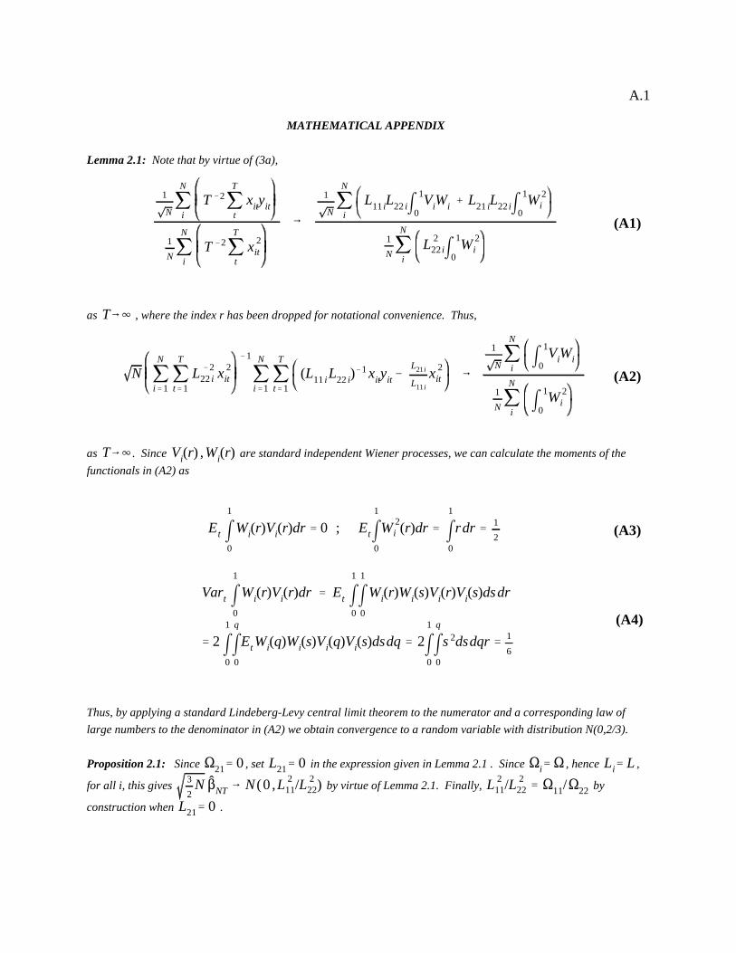
1

Nj

N

i

T &2jT

t

xityit

1

N jN

i

T &2jT

t

x 2it

6

1

Nj

N

i

L11 iL22 im1

0ViWi % L21 iL22 im

1

0W 2

i

1

N jN

i

L 222 im

1

0W 2

i

N jN

i'1j

T

t'1

L &222 i x 2

it

&1

jN

i'1j

T

t'1

(L11 iL22 i)&1 xityit&

L21 i

L11 i

x 2it 6

1

Nj

N

i m1

0ViWi

1

N jN

i m1

0W 2

i

Vart m1

0

Wi(r)Vi(r)dr ' Et m1

0m1

0

Wi(r)Wi(s)Vi(r)Vi(s)dsdr

' 2 m1

0mq

0

Et Wi(q)Wi(s)Vi(q)Vi(s)dsdq ' 2m1

0mq

0

s 2dsdqr ' 1

6

Et m1

0

Wi(r)Vi(r)dr ' 0 ; Etm1

0

W 2i (r)dr ' m

1

0

rdr ' 1

2

T64

T64 Vi(r) ,Wi(r)

S21' 0 L21' 0 Si' S Li' L3

2N $NT 6 N (0 ,L 2

11/L222) L 2

11/L222 ' S11/S22

L21' 0

A.1

(A1)

(A2)

(A4)

(A3)

MATHEMATICAL APPENDIX

Lemma 2.1: Note that by virtue of (3a),

as , where the index r has been dropped for notational convenience. Thus,

as . Since are standard independent Wiener processes, we can calculate the moments of the

functionals in (A2) as

Thus, by applying a standard Lindeberg-Levy central limit theorem to the numerator and a corresponding law of

large numbers to the denominator in (A2) we obtain convergence to a random variable with distribution N(0,2/3).

Proposition 2.1: Since , set in the expression given in Lemma 2.1 . Since , hence ,

for all i, this gives by virtue of Lemma 2.1. Finally, by

construction when .

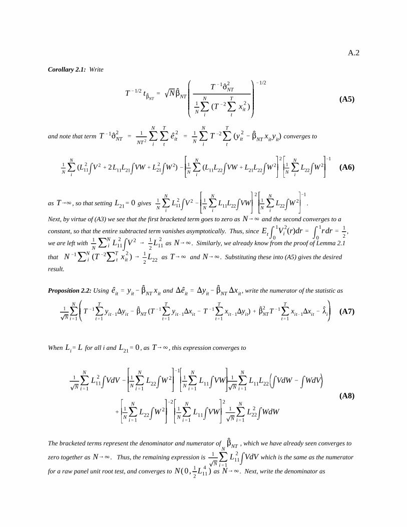
T &1/2 t $NT' N $NT

T &1F2NT

1

N jN

i

(T &2jT

t

x 2it )

&1/2

1

N jN

i(L 2

11mV 2 % 2L11L21mVW % L 221mW 2) & 1

N jN

i(L11L22mVW % L21L22mW 2

21

N jN

iL22mW 2

&1

1

NjN

i'1T &1j

T

t'1yit&1)yit & $NT (T &1j

T

t'1yit&1)xit & T &1j

T

t'1xit&1)yit) % $2

NTT &1jT

t'1xit&1)xit & 8i

1

NjN

i'1

L 211mVdV &

1

N jN

i'1

L22mW 2

&11

N jN

i'1

L11mVW 1

NjN

i'1

L11L22 mVdW & mWdV

%1

N jN

i'1

L22mW 2

&21

N jN

i'1

L11mVW2

1

NjN

i'1

L 222mWdW

T &1F2NT '

1

NT 2 jN

ij

T

t

e 2it '

1

N jN

i

T &2jT

t

(y 2it & $NT xit yit)

T64 L21' 0 1

N jN

iL 2

11mV 2 &1

N jN

iL11L22mVW

21

N jN

iL22mW 2

&1

N64

Etm1

0V 2

i (r)dr ' m1

0rdr ' 1

21

N jNi L 2

11mV 2 6 1

2L 2

11 N64

N &1jNi (T &2jT

t x 2it ) 6 1

2L22 T64 N64

eit ' yit& $NT xit )eit ' )yit& $NT )xit

Li' L L21' 0 T64

$NT

N64 1

Nj

N

i'1

L 211mVdV

N( 0 , 1

2L 4

11 ) N64

A.2

(A5)

(A6)

(A7)

(A8)

Corollary 2.1: Write

and note that term converges to

as , so that setting gives .

Next, by virtue of (A3) we see that the first bracketed term goes to zero as and the second converges to a

constant, so that the entire subtracted term vanishes asymptotically. Thus, since ,

we are left with as . Similarly, we already know from the proof of Lemma 2.1

that as and . Substituting these into (A5) gives the desired

result.

Proposition 2.2: Using and , write the numerator of the statistic as

When for all i and , as , this expression converges to

The bracketed terms represent the denominator and numerator of , which we have already seen converges to

zero together as . Thus, the remaining expression is which is the same as the numerator

for a raw panel unit root test, and converges to as . Next, write the denominator as

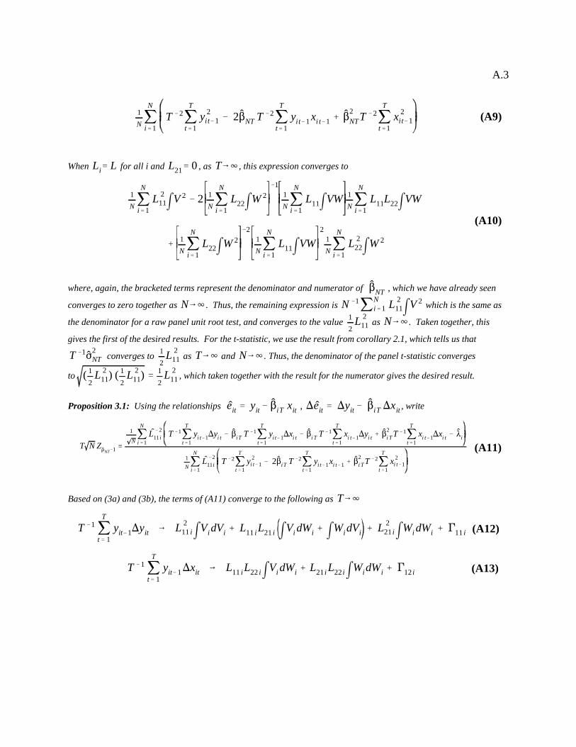
1

N jN

i'1T &2j

T

t'1y 2

i t&1 & 2$NT T &2jT

t'1yi t&1 xi t&1 % $2

NTT &2jT

t'1x 2

i t&1

1

N jN

i'1L 2

11mV 2 & 2 1

N jN

i'1L22mW 2

&11

N jN

i'1L11mVW 1

N jN

i'1L11L22mVW

%1

N jN

i'1L22mW 2

&21

N jN

i'1L11mVW

21

N jN

i'1L 2

22mW 2

T N ZDNT&1 /

1

NjN

i'1

L&211 i T &1j

T

t'1

yi t&1)yi t & $iT T &1jT

t'1

yi t&1)xi t & $i T T &1jT

t'1

xi t&1)yi t % $2i T T &1j

T

t'1

xi t&1)xi t & 8i

1

N jN

i'1L

&211i T &2j

T

t'1y 2

i t&1 & 2$iT T &2jT

t'1yi t&1xi t&1 % $2

i T T &2jT

t'1x 2

i t&1

T &1 jT

t' 1yit&1)yit 6 L 2

11 imVidVi % L11 iL21 i mVi dWi % mWidVi % L 221 imWi dWi % '11 i

T &1 jT

t' 1

yit&1)xit 6 L11 iL22 imVi dWi % L21 i L22 imWidWi % '12 i

Li' L L21' 0 T64

$NT

N64 N &1jNi'1 L 2

11mV 2

1

2L 2

11 N64

T &1F2NT

1

2L 2

11 T64 N64

( 1

2L 2

11) ( 1

2L 2

11) '1

2L 2

11

eit ' yit& $iT xit )eit ' )yit& $iT )xit

T64

A.3

(A9)

(A10)

(A11)

(A12)

(A13)

When for all i and , as , this expression converges to

where, again, the bracketed terms represent the denominator and numerator of , which we have already seen

converges to zero together as . Thus, the remaining expression is which is the same as

the denominator for a raw panel unit root test, and converges to the value as . Taken together, this

gives the first of the desired results. For the t-statistic, we use the result from corollary 2.1, which tells us that

converges to as and . Thus, the denominator of the panel t-statistic converges

to , which taken together with the result for the numerator gives the desired result.

Proposition 3.1: Using the relationships , , write

Based on (3a) and (3b), the terms of (A11) converge to the following as

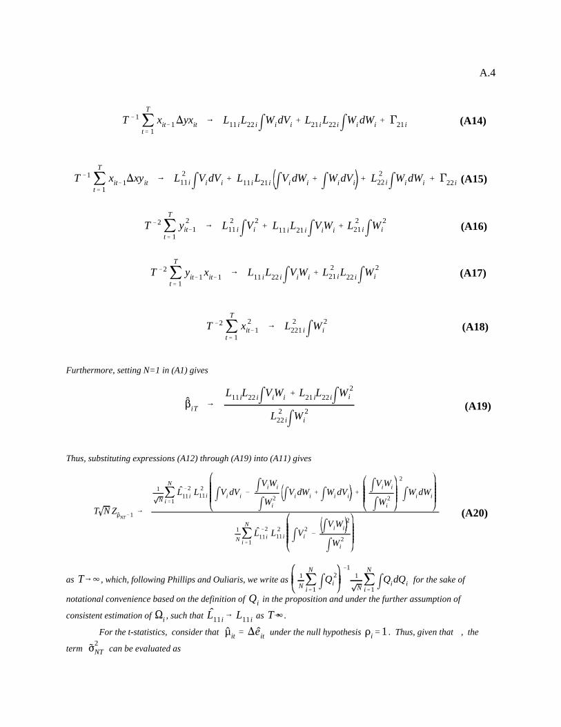
T &1 jT

t' 1

xit&1)yxit 6 L11 iL22 imWidVi % L21 i L22 imWi dWi % '21 i

T &2 jT

t' 1

x 2it&1 6 L 2

221 imW 2i

T &2 jT

t' 1

yit&1 xit&1 6 L11 iL22 imViWi % L 221 iL22 imW 2

i

T &2 jT

t' 1y 2

it&1 6 L 211 imV 2

i % L11 iL21 imViWi % L 221 imW 2

i

T &1 jT

t' 1

xit&1)xyit 6 L 211 imVidVi % L11 i L21 i mVi dWi % mWidVi % L 2

22 imWi dWi % '22 i

$iT 6L11 iL22 imViWi % L21 iL22 imW 2

i

L 222 imW 2

i

T N ZDNT&1 6

1

Nj

N

i'1L &2

11 i L 211 i mVi dVi &

mViWi

mW2i

mVi dWi % mWi dVi % mViWi

mW 2i

2

mWi dWi

1

N jN

i'1L &2

11 i L 211 i mV 2

i & mViWi2

mW 2i

T64 1

N jN

i'1 mQ 2i

&11

NjN

i'1 mQidQi

Qi

Si L11 i 6 L11 i T64

µ it ' )eit Di'1

F2NT

A.4

(A14)

(A18)

(A17)

(A16)

(A15)

(A19)

(A20)

Furthermore, setting N=1 in (A1) gives

Thus, substituting expressions (A12) through (A19) into (A11) gives

as , which, following Phillips and Ouliaris, we write as for the sake of

notational convenience based on the definition of in the proposition and under the further assumption of

consistent estimation of , such that as .

For the t-statistics, consider that under the null hypothesis . Thus, given that , the

term can be evaluated as

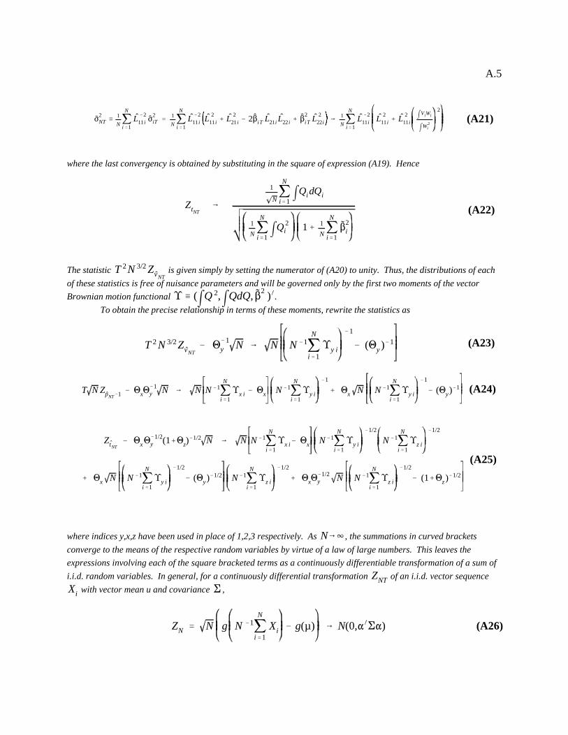
F2NT / 1

N jN

i'1L

&211 i F

2iT '

1

N jN

i'1L

&211 i L

211 i % L

221 i & 2$iT L21i L22 i % $2

iT L2

22i 6 1

N jN

i'1L

&211i L

211 i % L

211i

mViWi

mW2i

2

ZtNT6

1

NjN

i'1 mQidQi

1

N jN

i'1 mQ 2i 1% 1

N jN

i'1$2

i

T 2 N 3/2 ZvNT& 1&1

y N 6 N N &1jN

i'1

Ky i

&1

& (1y )&1

T N ZpNT&1 & 1x1&1y N 6 N N &1j

N

i'1Kx i & 1x N &1j

N

i'1Ky i

&1

% 1x N N &1jN

i'1Ky i

&1

& (1y)&1

ZtNT& 1x1

&1/2y (1%1z)

&1/2 N 6 N N &1jN

i'1Kx i& 1x N&1j

N

i'1Ky i

&1/2

N &1jN

i'1Kz i

&1/2

% 1x N N &1jN

i'1Ky i

&1/2

& (1y)&1/2 N&1jN

i'1Kz i

&1/2

% 1x1&1/2y N N &1j

N

i'1Kz i

&1/2

& (1%1z)&1/2

ZN ' N g N &1jN

i'1Xi & g(µ) 6 N(0,")E")

T 2 N 3/2 ZvNT

K / (mQ 2,mQdQ, $2))

N64

ZNTXi E

A.5

(A21)

(A22)

(A23)

(A24)

(A25)

(A26)

where the last convergency is obtained by substituting in the square of expression (A19). Hence

The statistic is given simply by setting the numerator of (A20) to unity. Thus, the distributions of each

of these statistics is free of nuisance parameters and will be governed only by the first two moments of the vector

Brownian motion functional .

To obtain the precise relationship in terms of these moments, rewrite the statistics as

where indices y,x,z have been used in place of 1,2,3 respectively. As , the summations in curved brackets

converge to the means of the respective random variables by virtue of a law of large numbers. This leaves the

expressions involving each of the square bracketed terms as a continuously differentiable transformation of a sum of

i.i.d. random variables. In general, for a continuously differential transformation of an i.i.d. vector sequence

with vector mean u and covariance ,

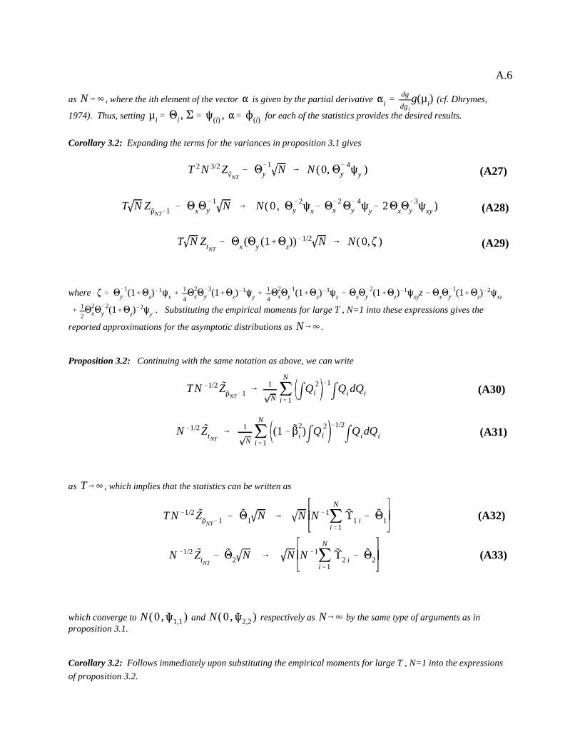
T N ZDNT&1 & 1x1&1y N 6 N( 0 , 1&2

y Rx& 1&2x 1& 4

y Ry& 21x1&3y Rxy )

T 2 N 3/2 ZvNT& 1&1

y N 6 N (0, 1& 4y Ry )

T N ZtNT& 1x (1y (1%1z))

&1/2 N 6 N( 0,. )

TN &1/2 ZDNT&1 6 1

NjN

i'1 mQ 2i

&1

mQi dQi

N &1/2 ZtNT6 1

Nj

N

i'1(1& $2

i )mQ 2i

&1/2

mQidQi

TN &1/2 ZDNT&1 & 11 N 6 N N &1jN

i'1K1 i & 11

N &1/2 ZtNT& 12 N 6 N N &1j

N

i'1K2 i & 12

N64 " "i 'dg

dg i

g(µ i)

µ i' 1i , E' R(i) , "' N(i)

. ' 1&1y (1%1z)

&1Rx %1

412

x1&3y (1%1z)

&1Ry %1

412

x1&1y (1%1z)

&3Rz & 1x1&2y (1%1z)

&1Rxyz &1x1&1y (1%1z)

&2Rxz

%1

212

x1&2y (1%1z)

&2Ry

N64

T64

N( 0 , R1,1 ) N( 0 , R2,2 ) N64

A.6

(A28)

(A27)

(A29)

(A30)

(A31)

(A32)

(A33)

as , where the ith element of the vector is given by the partial derivative (cf. Dhrymes,

1974). Thus, setting for each of the statistics provides the desired results.

Corollary 3.2: Expanding the terms for the variances in proposition 3.1 gives

where

. Substituting the empirical moments for large T , N=1 into these expressions gives the

reported approximations for the asymptotic distributions as .

Proposition 3.2: Continuing with the same notation as above, we can write

as , which implies that the statistics can be written as

which converge to and respectively as by the same type of arguments as inproposition 3.1.

Corollary 3.2: Follows immediately upon substituting the empirical moments for large T , N=1 into the expressions

of proposition 3.2.

(' 0 F ' 0.25 F ' 1 F ' 42 '

(' 0.8 F ' 0.25 F ' 1 F ' 42 '

(' 0 F ' 0.25 F ' 1 F ' 42 '

(' 0.8 F ' 0.25 F ' 1 F ' 42 '

B.1

Table 1. Empirical Size for 5% level tests under the null of no cointegration, N=20,T=100.

-0.5 0 0.5 -0.5 0 0.5 -0.5 0 0.5 panel v 0.022 0.021 0.021 0.021 0.023 0.019 0.022 0.018 0.019

panel rho 0.073 0.074 0.074 0.079 0.077 0.081 0.082 0.075 0.059

panel pp 0.076 0.077 0.077 0.076 0.087 0.081 0.083 0.075 0.067

panel adf 0.108 0.104 0.105 0.108 0.128 0.124 0.126 0.113 0.116

group rho 0.054 0.056 0.056 0.055 0.056 0.056 0.059 0.059 0.057

group pp 0.080 0.082 0.082 0.085 0.100 0.096 0.100 0.089 0.089

group adf 0.300 0.302 0.302 0.296 0.300 0.300 0.301 0.292 0.299

-0.5 0 0.5 -0.5 0 0.5 -0.5 0 0.5 panel v 0.010 0.003 0.002 0.032 0.012 0.013 0.042 0.019 0.035

panel rho 0.033 0.021 0.020 0.059 0.037 0.046 0.061 0.031 0.048

panel pp 0.034 0.018 0.021 0.057 0.034 0.049 0.068 0.039 0.055

panel adf 0.040 0.014 0.016 0.079 0.038 0.060 0.088 0.036 0.081

group rho 0.011 0.003 0.003 0.046 0.016 0.030 0.066 0.026 0.068

group pp 0.025 0.006 0.005 0.076 0.032 0.051 0.101 0.046 0.103

group adf 0.109 0.024 0.020 0.234 0.108 0.173 0.307 0.152 0.318

Table 2. Empirical Size for 5% level tests under the null of no cointegration, N=20,T=250.

-0.5 0 0.5 -0.5 0 0.5 -0.5 0 0.5

panel v 0.038 0.038 0.038 0.036 0.036 0.036 0.036 0.036 0.037

panel rho 0.071 0.068 0.069 0.068 0.067 0.061 0.065 0.056 0.068

panel pp 0.059 0.060 0.060 0.055 0.051 0.045 0.050 0.048 0.049

panel adf 0.069 0.070 0.070 0.074 0.067 0.062 0.064 0.055 0.060

group rho 0.065 0.067 0.066 0.072 0.074 0.068 0.070 0.065 0.067

group pp 0.059 0.061 0.061 0.068 0.065 0.062 0.065 0.059 0.060

group adf 0.140 0.139 0.139 0.143 0.148 0.135 0.141 0.131 0.134

-0.5 0 0.5 -0.5 0 0.5 -0.5 0 0.5 panel v 0.024 0.007 0.005 0.046 0.026 0.028 0.054 0.033 0.048

panel rho 0.043 0.029 0.024 0.050 0.031 0.041 0.047 0.036 0.057

panel pp 0.036 0.025 0.022 0.038 0.026 0.034 0.036 0.032 0.045

panel adf 0.025 0.009 0.011 0.041 0.008 0.028 0.039 0.015 0.044

group rho 0.027 0.006 0.005 0.062 0.028 0.044 0.077 0.035 0.075

group pp 0.030 0.015 0.014 0.056 0.027 0.042 0.065 0.040 0.067

group adf 0.041 0.011 0.011 0.106 0.031 0.074 0.140 0.048 0.140

(' 0 F ' 0.25 F ' 1 F ' 42 '

(' 0.8 F ' 0.25 F ' 1 F ' 42 '

D'1 a'1(, F, 2

a' 0 ( ' 0 ( ' 0.8 ( ' &0.82 '

D'1 a'0 F ' 1 (, 2

B.2

Table 3. Empirical Size for 5% level tests under the null of no cointegration, N=20,T=20.

-0.5 0 0.5 -0.5 0 0.5 -0.5 0 0.5

panel v 0.000 0.000 0.000 0.000 0.000 0.000 0.000 0.000 0.000panel rho 0.041 0.041 0.041 0.042 0.040 0.038 0.040 0.033 0.035panel pp 0.233 0.235 0.235 0.225 0.241 0.228 0.235 0.220 0.228panel adf 0.213 0.218 0.218 0.227 0.226 0.218 0.231 0.208 0.220group rho 0.001 0.001 0.001 0.002 0.001 0.000 0.000 0.001 0.000group pp 0.220 0.221 0.221 0.222 0.228 0.222 0.228 0.221 0.226group adf 0.444 0.444 0.445 0.441 0.446 0.439 0.452 0.426 0.445

-0.5 0 0.5 -0.5 0 0.5 -0.5 0 0.5

panel v 0.000 0.000 0.000 0.000 0.000 0.000 0.000 0.000 0.000panel rho 0.013 0.001 0.001 0.040 0.012 0.017 0.041 0.016 0.041panel pp 0.105 0.042 0.038 0.206 0.106 0.134 0.244 0.142 0.244panel adf 0.088 0.027 0.024 0.185 0.081 0.107 0.221 0.110 0.213group rho 0.000 0.000 0.000 0.001 0.000 0.000 0.002 0.000 0.002group pp 0.049 0.006 0.004 0.175 0.075 0.117 0.272 0.143 0.294group adf 0.142 0.036 0.030 0.363 0.188 0.259 0.494 0.294 0.516

Notes: (for Tables 1-3). Based on 2000 draws each for DGP 4.1, with , and varying as indicated. Number of lags set to K=1,5,7 for T=20,100,250 respectively.

Table 4. Empirical Size for 5% level tests under the null of no cointegration, N=20,T=20.

-0.5 0 0.5 -0.5 0 0.5 -0.5 0 0.5

panel v 0.000 0.000 0.000 0.000 0.000 0.000 0.000 0.000 0.000panel rho 0.035 0.039 0.038 0.021 0.046 0.039 0.001 0.001 0.003panel pp 0.209 0.230 0.228 0.143 0.246 0.243 0.036 0.036 0.030panel adf 0.195 0.215 0.218 0.105 0.219 0.215 0.068 0.086 0.071group rho 0.000 0.001 0.000 0.000 0.002 0.002 0.000 0.000 0.000group pp 0.201 0.237 0.222 0.150 0.306 0.281 0.018 0.007 0.009group adf 0.424 0.450 0.439 0.309 0.525 0.515 0.088 0.070 0.065

Notes: Based on 2000 draws each for DGP 4.1, with , , and varying asindicated. Number of lags set to K=1.

F2'1,2'0 ( ~ U(0, 0.4) ( ~ U(0, 0.8) ( ~ U(&0.4, 0.4)T '

D'1 a'1 F2'1, 2'0 (

F~U(0.25,4)2~U(&0.5,0.5) ( ' 0 ( ' 0.8 ( ~ U(0, 0.8)

T '

D'1 a'1 F2 F2~U(0.25,4) 22~U(&0.5,0.5) (

F'1,2'0 ( ~ U(&0.4,0.4) ( ~ U(&0.4,0) ( ~ U(&0.4,0.8) ( ~ U(&0.8,0.8)a '

D'1 F2'1, 2'0 a(

B.3

Table 5. Empirical Size for 5% level tests under the null of no cointegration, N=20.

20 100 250 20 100 250 20 100 250

panel v 0.000 0.015 0.032 0.000 0.015 0.030 0.000 0.042 0.075panel rho 0.021 0.044 0.046 0.015 0.042 0.040 0.091 0.157 0.126panel pp 0.151 0.054 0.033 0.129 0.049 0.032 0.367 0.156 0.102panel adf 0.128 0.059 0.024 0.101 0.047 0.019 0.404 0.277 0.234group rho 0.000 0.025 0.035 0.000 0.018 0.029 0.006 0.277 0.244group pp 0.129 0.046 0.036 0.102 0.040 0.033 0.416 0.287 0.186group adf 0.288 0.148 0.050 0.241 0.121 0.039 0.686 0.687 0.514

Notes: Based on 2000 draws each for DGP 4.1, with , , , T varying and drawnfrom various uniform distributions as indicated. Lags K=1,5,7 for T=20,100,250.

Table 6. Empirical Size for 5% level tests under the null of no cointegration, N=20.

20 100 250 20 100 250 20 100 250

panel v 0.000 0.023 0.037 0.000 0.013 0.031 0.000 0.018 0.040panel rho 0.043 0.072 0.067 0.016 0.023 0.041 0.026 0.046 0.049panel pp 0.240 0.078 0.048 0.133 0.029 0.030 0.169 0.046 0.040panel adf 0.233 0.110 0.060 0.094 0.032 0.018 0.152 0.057 0.025group rho 0.000 0.052 0.063 0.000 0.014 0.026 0.000 0.028 0.039group pp 0.230 0.085 0.058 0.096 0.033 0.027 0.154 0.054 0.040group adf 0.455 0.288 0.133 0.218 0.112 0.035 0.318 0.164 0.057

Notes: Based on 2000 draws each for DGP 4.1, with , , drawn from , drawn from and T and varying as indicated. Lags K=1,5,7 respectively.

Table 7. Empirical Size for 5% level tests under the null of no cointegration, N=20, T=20.

0 1 0 1 0 1 0 1

panel v 0.000 0.000 0.000 0.000 0.000 0.000 0.000 0.000panel rho 0.041 0.091 0.049 0.251 0.038 0.056 0.028 0.331panel pp 0.220 0.367 0.247 0.586 0.201 0.273 0.175 0.674panel adf 0.229 0.404 0.277 0.648 0.192 0.284 0.203 0.740group rho 0.001 0.006 0.001 0.035 0.001 0.001 0.000 0.115group pp 0.207 0.416 0.227 0.659 0.195 0.308 0.150 0.846group adf 0.455 0.686 0.499 0.890 0.425 0.548 0.375 0.969

Notes: Based on 2000 draws each for DGP 4.1, with , , varying as indicatedand drawn from various uniform distributions as indicated. Lags set to K=1.

D'0.9

(' 0 F ' 0.25 F ' 1 F ' 42 '

(' 0.8 F ' 0.25 F ' 1 F ' 42 '

D'0.9

(' 0 F ' 0.25 F ' 1 F ' 42 '

(' 0.8 F ' 0.25 F ' 1 F ' 42 '

B.4

Table 8. Power of 5% level tests against alternate when , N=20,T=100.

-0.5 0 0.5 -0.5 0 0.5 -0.5 0 0.5 panel v 0.000 0.005 0.001 0.086 0.989 1.000 0.988 1.000 1.000

panel rho 0.036 0.185 0.122 0.950 1.000 1.000 1.000 1.000 1.000

panel pp 0.039 0.163 0.123 0.901 0.999 1.000 0.999 1.000 1.000

panel adf 0.094 0.339 0.247 0.972 1.000 1.000 1.000 1.000 1.000

group rho 0.007 0.064 0.018 0.762 0.994 1.000 0.997 1.000 1.000

group pp 0.018 0.103 0.036 0.810 0.994 1.000 0.998 1.000 1.000

group adf 0.129 0.446 0.245 0.978 1.000 1.000 1.000 1.000 1.000

-0.5 0 0.5 -0.5 0 0.5 -0.5 0 0.5 panel v 0.000 0.011 0.002 0.863 1.000 1.000 1.000 1.000 1.000

panel rho 0.364 0.603 0.581 1.000 1.000 1.000 1.000 1.000 1.000

panel pp 0.294 0.493 0.465 0.993 1.000 1.000 1.000 1.000 1.000

panel adf 0.533 0.660 0.582 0.999 1.000 1.000 1.000 1.000 1.000

group rho 0.093 0.168 0.104 0.987 0.999 1.000 1.000 1.000 1.000

group pp 0.164 0.245 0.155 0.992 0.999 1.000 1.000 1.000 1.000

group adf 0.556 0.581 0.438 1.000 1.000 1.000 1.000 1.000 1.000

Table 9. Power of 5% level tests against alternate when , N=20,T=250.

-0.5 0 0.5 -0.5 0 0.5 -0.5 0 0.5 panel v 0.000 0.074 0.003 1.000 1.000 1.000 1.000 1.000 1.000

panel rho 0.972 1.000 1.000 1.000 1.000 1.000 1.000 1.000 1.000

panel pp 0.924 0.998 0.993 1.000 1.000 1.000 1.000 1.000 1.000

panel adf 0.993 1.000 1.000 1.000 1.000 1.000 1.000 1.000 1.000

group rho 0.629 0.973 0.960 1.000 1.000 1.000 1.000 1.000 1.000

group pp 0.632 0.967 0.926 1.000 1.000 1.000 1.000 1.000 1.000

group adf 0.934 1.000 0.995 1.000 1.000 1.000 1.000 1.000 1.000

-0.5 0 0.5 -0.5 0 0.5 -0.5 0 0.5 panel v 0.077 0.914 0.790 1.000 1.000 1.000 1.000 1.000 1.000

panel rho 1.000 1.000 1.000 1.000 1.000 1.000 1.000 1.000 1.000

panel pp 1.000 1.000 1.000 1.000 1.000 1.000 1.000 1.000 1.000

panel adf 1.000 1.000 1.000 1.000 1.000 1.000 1.000 1.000 1.000

group rho 1.000 1.000 1.000 1.000 1.000 1.000 1.000 1.000 1.000

group pp 1.000 1.000 1.000 1.000 1.000 1.000 1.000 1.000 1.000

group adf 1.000 1.000 1.000 1.000 1.000 1.000 1.000 1.000 1.000

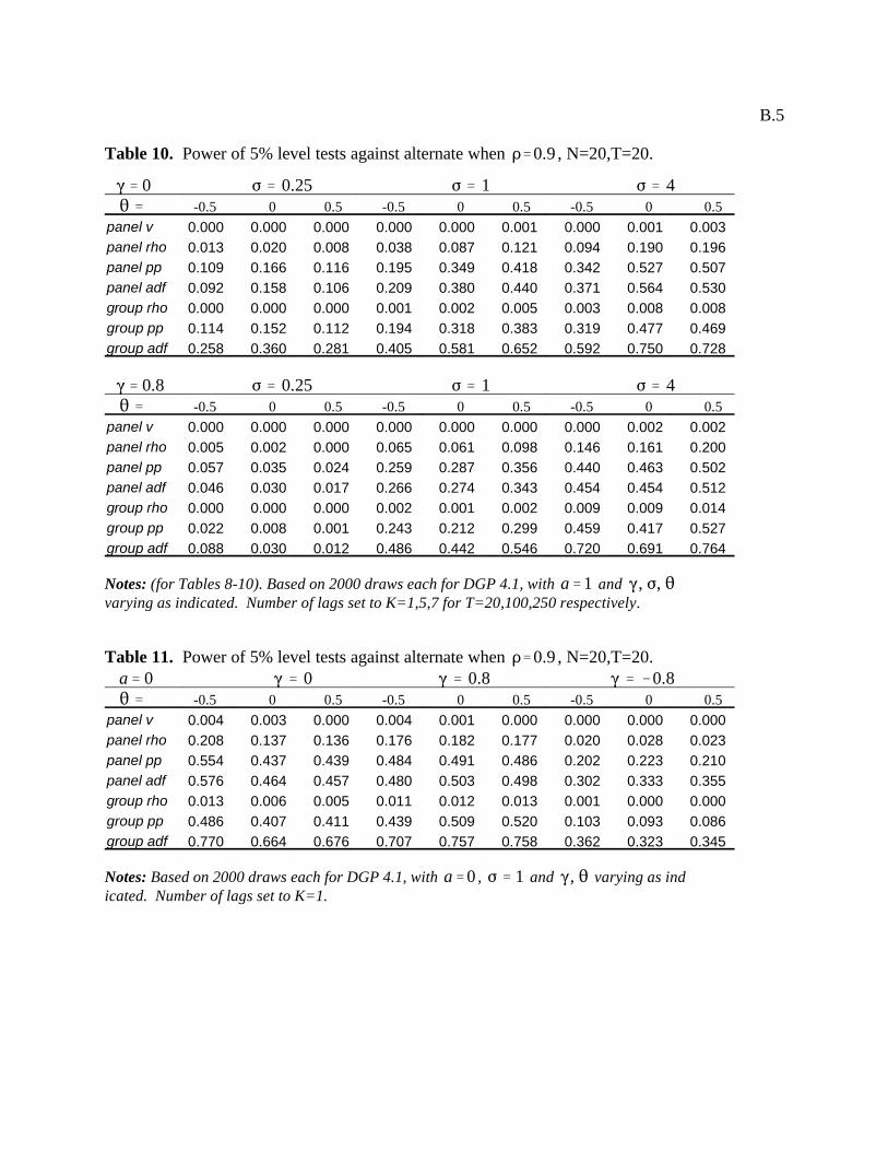
D'0.9

(' 0 F ' 0.25 F ' 1 F ' 42 '

(' 0.8 F ' 0.25 F ' 1 F ' 42 '

a'1 (, F, 2

D'0.9a' 0 ( ' 0 ( ' 0.8 ( ' &0.82 '

a'0 F ' 1 (, 2

B.5

Table 10. Power of 5% level tests against alternate when , N=20,T=20.

-0.5 0 0.5 -0.5 0 0.5 -0.5 0 0.5

panel v 0.000 0.000 0.000 0.000 0.000 0.001 0.000 0.001 0.003panel rho 0.013 0.020 0.008 0.038 0.087 0.121 0.094 0.190 0.196panel pp 0.109 0.166 0.116 0.195 0.349 0.418 0.342 0.527 0.507panel adf 0.092 0.158 0.106 0.209 0.380 0.440 0.371 0.564 0.530group rho 0.000 0.000 0.000 0.001 0.002 0.005 0.003 0.008 0.008group pp 0.114 0.152 0.112 0.194 0.318 0.383 0.319 0.477 0.469group adf 0.258 0.360 0.281 0.405 0.581 0.652 0.592 0.750 0.728

-0.5 0 0.5 -0.5 0 0.5 -0.5 0 0.5

panel v 0.000 0.000 0.000 0.000 0.000 0.000 0.000 0.002 0.002panel rho 0.005 0.002 0.000 0.065 0.061 0.098 0.146 0.161 0.200panel pp 0.057 0.035 0.024 0.259 0.287 0.356 0.440 0.463 0.502panel adf 0.046 0.030 0.017 0.266 0.274 0.343 0.454 0.454 0.512group rho 0.000 0.000 0.000 0.002 0.001 0.002 0.009 0.009 0.014group pp 0.022 0.008 0.001 0.243 0.212 0.299 0.459 0.417 0.527group adf 0.088 0.030 0.012 0.486 0.442 0.546 0.720 0.691 0.764

Notes: (for Tables 8-10). Based on 2000 draws each for DGP 4.1, with and varying as indicated. Number of lags set to K=1,5,7 for T=20,100,250 respectively.

Table 11. Power of 5% level tests against alternate when , N=20,T=20.

-0.5 0 0.5 -0.5 0 0.5 -0.5 0 0.5

panel v 0.004 0.003 0.000 0.004 0.001 0.000 0.000 0.000 0.000panel rho 0.208 0.137 0.136 0.176 0.182 0.177 0.020 0.028 0.023panel pp 0.554 0.437 0.439 0.484 0.491 0.486 0.202 0.223 0.210panel adf 0.576 0.464 0.457 0.480 0.503 0.498 0.302 0.333 0.355group rho 0.013 0.006 0.005 0.011 0.012 0.013 0.001 0.000 0.000group pp 0.486 0.407 0.411 0.439 0.509 0.520 0.103 0.093 0.086group adf 0.770 0.664 0.676 0.707 0.757 0.758 0.362 0.323 0.345

Notes: Based on 2000 draws each for DGP 4.1, with , and varying as indicated. Number of lags set to K=1.

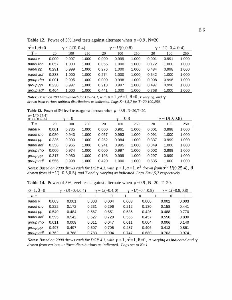
D'0.9

F2'1,2'0 ( ~ U(0, 0.4) ( ~ U(0, 0.8) ( ~ U(&0.4, 0.4)T '

a'1 F2'1, 2'0 (

D'0.9F~U(0.25,4)2~U(&0.5,0.5) ( ' 0 ( ' 0.8 ( ~ U(0, 0.8)

T '

D'1 a'1 F2 F2~U(0.25,4) 22~U(&0.5,0.5) (

D'0.9

F'1,2'0 ( ~ U(&0.4,0.4) ( ~ U(&0.4,0) ( ~ U(&0.4,0.8) ( ~ U(&0.8,0.8)a '

D'1 F2'1, 2'0 a (

B.6

Table 12. Power of 5% level tests against alternate when , N=20.

20 100 250 20 100 250 20 100 250

panel v 0.000 0.997 1.000 0.000 0.999 1.000 0.001 0.991 1.000panel rho 0.057 1.000 1.000 0.055 1.000 1.000 0.172 1.000 1.000panel pp 0.291 0.999 1.000 0.276 1.000 1.000 0.484 0.998 1.000panel adf 0.288 1.000 1.000 0.274 1.000 1.000 0.542 1.000 1.000group rho 0.001 0.995 1.000 0.000 0.998 1.000 0.008 0.996 1.000group pp 0.230 0.997 1.000 0.213 0.997 1.000 0.497 0.996 1.000group adf 0.464 1.000 1.000 0.441 1.000 1.000 0.768 1.000 1.000

Notes: Based on 2000 draws each for DGP 4.1, with , , T varying, and drawn from various uniform distributions as indicated. Lags K=1,5,7 for T=20,100,250.

Table 13. Power of 5% level tests against alternate when , N=20,T=20.

20 100 250 20 100 250 20 100 250

panel v 0.001 0.735 1.000 0.000 0.961 1.000 0.001 0.998 1.000panel rho 0.080 0.943 1.000 0.057 0.993 1.000 0.091 1.000 1.000panel pp 0.336 0.900 1.000 0.252 0.984 1.000 0.337 0.999 1.000panel adf 0.356 0.965 1.000 0.241 0.995 1.000 0.349 1.000 1.000group rho 0.000 0.974 1.000 0.000 0.997 1.000 0.002 0.999 1.000group pp 0.317 0.980 1.000 0.198 0.999 1.000 0.297 0.999 1.000group adf 0.556 0.998 1.000 0.420 1.000 1.000 0.535 1.000 1.000

Notes: Based on 2000 draws each for DGP 4.1, with , , drawn from , drawn from and T and varying as indicated. Lags K=1,5,7 respectively.

Table 14. Power of 5% level tests against alternate when , N=20, T=20.

0 1 0 1 0 1 0 1

panel v 0.003 0.001 0.003 0.004 0.003 0.000 0.002 0.003panel rho 0.222 0.172 0.231 0.296 0.212 0.130 0.158 0.441panel pp 0.549 0.484 0.567 0.651 0.536 0.426 0.488 0.770panel adf 0.595 0.542 0.627 0.728 0.565 0.457 0.550 0.830group rho 0.011 0.008 0.011 0.047 0.011 0.004 0.006 0.140group pp 0.497 0.497 0.507 0.705 0.487 0.406 0.413 0.861group adf 0.762 0.768 0.783 0.904 0.747 0.680 0.703 0.974

Notes: Based on 2000 draws each for DGP 4.1, with , , varying as indicated and drawn from various uniform distributions as indicated. Lags set to K=1.